Multirefringence phenomena in nonlinear electrodynamics

Abstract

Wave propagation in nonlinear theories of the electromagnetism described by Lagrangian densities dependent upon its two local invariants $L(F,G)$ is revisited. On the light of the recent findings in metamaterials, it is here shown that trirefringence is also a possible phenomenon to occur in the realm of such nonlinear theories. A specific model exhibiting this effect is investigated both in terms of phase and group velocities. It is claimed that wave propagation in some well known nonlinear models for spin-one fields, like QED and QCD in certain regimes, may exhibit trirefringence.

I Introduction

As it is well known, nonlinear theories of electromagnetism exhibit birefringence phenomenon. The most popular example appears in the quantum electrodynamics (QED) where polarization effects are activated in the limit of large fields ($B_{\scriptscriptstyle cr}\sim E_{\scriptscriptstyle cr}=m^{2}c^{3}/e\hbar$), inducing an effective optical axis in the vacuum. In such situation, a light ray is expected to split in two rays propagating with different velocities Birula ; Adler ; delorenci2000a ; delorenci2000b . An experimental setup designed to measure the birefringent properties of the QED vacuum was long ago proposed Iacoppini . However, direct measurements of this effect are not yet conclusive and are still under consideration valle2010 . The influence of the nontrivial vacua on the propagation of electromagnetic waves was discussed in several distinct physical configurations Latorre ; Drumond ; Shore ; Scharnhorst ; Barton ; Dittrich . Conditions for the occurrence of birefringence of gluon fields was also studied shi2008 .

In the context of material media, birefringence effects are expect to occur in several distinct situations. It occurs naturally, for instance in certain crystals presenting optical axes Landau ; born , or artificially when optical axes are induced by means of external applied electromagnetic fields delorenci2008 ; delorenci2004 . Nowadays, birefringent materials and methods including this effect have been incorporated in several technological devices paschotta2008 . Birefringence is also a powerful optical tool to investigate properties of new materials, biological systems and others bio ; astro1 ; astro2 .

On the other hand, trirefringence was only recently considered as a possible phenomenon in material media. It was measured tri1 in tailored photonic crystals Joannopoulos , and the theoretical description of this effect in media characterized by effective dielectric coefficients was proposed delorenci2012 . In this case delorenci2012 , only when some of the dielectric coefficients are negative, could trirefringence take place. Metamaterials smith2 ; smith ; veselago ; shelby seem to be good candidates for supporting this effect, due to the controllability of their dielectric tensors. With the present day technology of producing such new media, it is expected that trirefringence will play some important role in technology of optical systems, as birefringence has done.

Usually, effects occurring in the realm of Maxwell electromagnetism in material media are expected to occur in the realm of nonlinear electromagnetic theories. It is possible to build up analogue models between these two domains where the coefficients describing a specific dielectric medium are mapped as derivatives of the Lagrangian density describing a nonlinear theory. In this way, trirefringence should also be a possible effect in nonlinear electromagnetism. By deriving and using the general description for wave propagation in the limit of geometrical optics, in this paper we show that trirefringence is in fact a possible effect in nonlinear electrodynamics. It is not our purpose to set the general conditions a model must fulfill in order to present trirefringence, but only to show the effect as a possible one in the domain of nonlinear electromagnetism. A particular model is thus investigated where such phenomenon is shown to occur provided that convenient external fields are set. The phase and group velocities of the waves are derived, as well as the corresponding polarization vectors. A numerical example is graphically studied.

The model examined in the paper corresponds to the effective Lagrangian density for QED in the regime of large fields. The trirefringence phenomenon is shown to occur whenever the model applies, although its measurability requires the control of very large fields. A possible arena to search for this effect could be the special fluids recently produced by high energy collisions, as addressed later in the concluding section. Further, this model is also useful in the context of analogue models in material media, where the predicted effect could be tested on optical systems, for instance in metamaterials.

In the next section, nonlinear electromagnetism is briefly revisited and the field equations are presented in terms of the general two parameters Lagrangian density. In Sec. III, the corresponding wave propagation is examined. The eigenvalue problem is stated and solved, resulting in the general fourth degree equation for the phase velocities. This equation is solved for a specific nonlinear model in Sec. IV. The corresponding polarization states and the description of the effect in terms of group velocities are also discussed. Conclusions and final remarks are presented in Sec. V.

Throughout this paper we employ the Minkowski metric $\eta_{\mu\nu}={\rm diag}(+1,-1,-1,-1)$. The completely skew-symmetric tensor $\eta^{\alpha\beta\mu\nu}$ is defined by $\eta^{0123}=1$. We set the units such that the velocity of light in empty space is $c=1$.

II Nonlinear electrodynamics: field equations

Nonlinear Abelian theories for electromagnetism can be formulated by means of the general Lagrangian density $L=L(F,G)$, where $F$ and $G$ are the two local gauge invariants of the electromagnetic field. These invariants are defined in terms of the electromagnetic tensor field $F_{\mu\nu}$, and its dual

$$\raisebox{0.86108pt}{$\stackrel{{\scriptstyle*}}{{F}}$}{}_{\alpha\beta}=\frac{1}{2}\eta_{\alpha\beta}{}^{\sigma\tau}F_{\sigma\tau},$$ (1)

as

$$F = F^{\mu\nu}F_{\mu\nu}$$ (2)

$$G = F^{\mu\nu}\raisebox{0.86108pt}{$\stackrel{{\scriptstyle*}}{{F}}$}{}_{\mu\nu}.$$ (3)

In terms of the electric $\vec{E}$ and magnetic $\vec{B}$ field strengths we have $F=-2(E^{2}-B^{2})$ and $G=-4\vec{E}\cdot\vec{B}$.

The field equation can be obtained from the least action principle and it can be presented as delorenci2000a ,

$$2N^{\mu\nu\alpha\beta}F_{\alpha\beta,\nu}+L_{F}F^{\mu\nu}{}_{,\nu}=0,$$ (4)

where $N^{\mu\nu\alpha\beta}$ is defined by

$$N^{\mu\nu\alpha\beta} \doteq L_{FF}F^{\mu\nu}F^{\alpha\beta}+L_{GG}\raisebox{0.86108pt}{$\stackrel{{\scriptstyle*}}{{F}}$}{}^{\mu\nu}\raisebox{0.86108pt}{$\stackrel{{\scriptstyle*}}{{F}}$}{}^{\alpha\beta}$$ (5)

$$+L_{FG}\left(F^{\mu\nu}\raisebox{0.86108pt}{$\stackrel{{\scriptstyle*}}{{F}}$}{}^{\alpha\beta}+\raisebox{0.86108pt}{$\stackrel{{\scriptstyle*}}{{F}}$}{}^{\mu\nu}F^{\alpha\beta}\right).$$

Use is being made here of the notation $L_{X^{1}X^{2}\cdots X^{n}}=\partial^{n}L/\partial X^{1}\partial X^{2}\cdots\partial X^{n}$ previously introduced delorenci2000a , where each $X^{i}$ is one of the two invariants $F$ or $G$ upon which the Lagrangian $L$ arbitrarily depends. We notice that the above defined rank-4 tensor presents the following symmetries: $N^{\mu\nu\alpha\beta}=-N^{\nu\mu\alpha\beta}$, $N^{\mu\nu\alpha\beta}=-N^{\mu\nu\beta\alpha}$ and $N^{\mu\nu\alpha\beta}=N^{\alpha\beta\mu\nu}$.

In addition to Eq. (4), $F_{\mu\nu}$ satisfies the Bianchi identity $\raisebox{0.86108pt}{$\stackrel{{\scriptstyle*}}{{F}}$}{}^{\mu\nu}{}_{,\nu}=0$, which implies in the existence of a potential vector $A_{\mu}$ as

$$F_{\mu\nu}=A_{\mu,\nu}-A_{\nu,\mu}.$$ (6)

III Nonlinear electrodynamics: wave propagation

Let us now discuss the propagation of electromagnetic waves in the general formulation of nonlinear electrodynamics. We restrict ourselves to the propagation of monochromatic waves in the limit imposed by geometrical optics Landau ; born . The method of field discontinuities will be used, which can be briefly stated as follows Hadamard ; delorenci2000a .

Consider a differentiable inextendible oriented borderless hypersurface $\Sigma$, defined locally by $\phi(x^{\mu})=0$, where $\phi$ is a real differentiable scalar field which locally is a function of the spacetime coordinates $x^{\mu}=(t,\vec{x})$. Let $U^{{}+{}}$ be the spacetime points whose coordinates satisfy $\phi(x^{\mu})>0$, and similarly $U^{{}-{}}$ be such that $\phi(x^{\mu})<0$. Let $P$ be any given point of $\Sigma$. For each sufficiently small $r>0$, let $V_{r}(P)$ be a neighborhood of $P$ which consists of the spacetime points $Q$ whose Euclidean distance from $P$ is $[(t_{Q}-t_{P})^{2}+||\vec{x}{}_{Q}-\vec{x}{}_{P}||^{2}]^{(1/2)}$ smaller than $r$. Let $P^{{}+{}}\in U^{{}+{}}\cap V_{r}(P)$ and $P^{{}-{}}\in U^{{}-{}}\cap V_{r}(P)$ be any two neighbor points from $P$ arbitrarily chosen at opposite sides of $\Sigma$. Let $f$ be any given tensor field defined at $V_{r}(P)$. The Hadamard discontinuity at $P$ of $f$ across $\Sigma$ is defined as

$$[f]_{\Sigma}(P)\doteq\lim_{r\rightarrow 0^{{}+{}}}\left[f(P^{{}+{}})-f(P^{{}-{}})\right].$$ (7)

Suppose $f$ such that $[f]_{\Sigma}=0$ for each $P\in\Sigma$. Following Hadamard Hadamard , we have $[f_{,\lambda}]_{\Sigma}(P)=k_{\lambda}\bar{f}(P)$, where $k_{\lambda}=\phi_{,\lambda}|_{P}$ is the normal vector to $\Sigma$ at $P$ and $\bar{f}$ is a tensor field defined at $\Sigma$ with the same rank and the same algebraic symmetries as those of $f$.

We assume the electromagnetic tensor field $F_{\mu\nu}$ to be smooth in each $U^{\pm}$, but merely continuous at $\Sigma$ (that is to say, the $F_{\mu\nu}$ are continuous functions at $\Sigma$ but their derivatives may present discontinuities at $\Sigma$). The Hadamard discontinuities at $\Sigma$ of Eq. (4) and of the derivative of Eq. (6) lead to delorenci2000a

$$f_{\beta\lambda}k^{\lambda}+\frac{2}{L_{F}}N_{\beta}{}^{\mu\nu\rho}f_{\nu\rho}k_{\mu}=0$$ (8)

and

$$f_{\alpha\beta}=\epsilon_{\alpha}k_{\beta}-\epsilon_{\beta}k_{\alpha},$$ (9)

where the quantities $f_{\alpha\beta}$ are related to the derivatives of $F_{\alpha\beta}$ on $\Sigma$ by $[F_{\alpha\beta,\lambda}]_{\Sigma}=f_{\alpha\beta}k_{\lambda}$ and $\epsilon_{\mu}$ is the polarization vector $[A_{\mu,\alpha\beta}]_{{}_{\Sigma}}=e_{\mu}k_{\alpha}k_{\beta}$. We set $k_{\lambda}=\omega V_{\lambda}+q_{\lambda}$ as the wave 4-vector, where $V_{\lambda}=\delta^{0}_{\lambda}$ is the 4-velocity of the observer which decomposes $F^{\mu\nu}$ into electric and magnetic fields. The components of this 4-vector $k_{\lambda}$ are thus the frequency $\omega$ and the wave vector $\vec{q}=q\hat{q}$, where $\|\hat{q}\|^{2}=-\hat{q}^{\lambda}\hat{q}_{\lambda}=1$.

Taking together Eqs. (8) and (9), we obtain the general eigenvalue equation Birula ; delorenci2000a

$$Z^{\mu}{}_{\nu}\epsilon^{\nu}=0,$$ (10)

where

$$Z^{\mu}{}_{\nu}\doteq k^{2}\delta^{\mu}{}_{\nu}+\frac{4}{L_{F}}N^{\mu\alpha}{}_{\nu\beta}k_{\alpha}k^{\beta},$$ (11)

with $k^{2}\doteq k^{\lambda}k_{\lambda}$. Nontrivial solutions of Eq. (10) can be found only if $\det\mid Z_{\mu\nu}\mid\,=\,0$, the well known generalized Fresnel equation, and yields

$$\alpha(k^{2})^{2}+\beta f^{2}k^{2}+\gamma(f^{2})^{2}=0,$$ (12)

where $f^{2}\doteq F^{\alpha\mu}F_{\alpha}{}^{\nu}k_{\mu}k_{\nu}$, and

$$\alpha = L_{F}^{2}+2L_{F}(GL_{FG}-FL_{GG})$$ (13)

$$-(L_{FF}L_{GG}-L_{FG}^{2})G^{2},$$

$$\beta = 4L_{F}(L_{FF}+L_{GG})-8(L_{FF}L_{GG}-L_{FG}^{2})F,$$ (14)

$$\gamma = 16(L_{FF}L_{GG}-L_{FG}^{2}).$$ (15)

One can also recast the quantity $f^{2}$ that appears in Eq. (12) as

$$f^{2}=(\vec{q}\cdot\vec{E})^{2}-\omega^{2}E^{2}+(\hat{q}\cdot\vec{B})^{2}-q^{2}B^{2}+2\omega\vec{q}\cdot\vec{E}\times\vec{B}.$$ (16)

The phase velocity $v\doteq\omega/q$ of the electromagnetic waves can be obtained from Eq. (12). In fact, it is straightforward to show that this equation can be presented as a fourth-degree equation for the phase velocity $v$ as

$$a_{4}v^{4}+a_{3}v^{3}+a_{2}v^{2}+a_{1}v+a_{0}=0,$$ (17)

where we have defined

$$a_{4} \doteq \alpha-\beta E^{2}+\gamma E^{4}$$ (18)

$$a_{3} \doteq 2(\beta-2\gamma E^{2})\hat{q}\cdot\vec{E}\times\vec{B}$$ (19)

$$a_{2} \doteq -2\alpha+\beta[E^{2}-B^{2}+(\hat{q}\cdot\vec{E})^{2}+(\hat{q}\cdot\vec{B})^{2}]$$ (20)

$$+2\gamma\{2(\hat{q}\cdot\vec{E}\times\vec{B})^{2}-[(\hat{q}\cdot\vec{E})^{2}+(\hat{q}\cdot\vec{B})^{2}$$

$$-B^{2}]E^{2}\}$$

$$a_{1} \doteq -2\{\beta-2\gamma[(\hat{q}\cdot\vec{E})^{2}+(\hat{q}\cdot\vec{B})^{2}$$ (21)

$$-B^{2}]\}\hat{q}\cdot\vec{E}\times\vec{B}$$

$$a_{0} \doteq \alpha+\beta[B^{2}-(\hat{q}\cdot\vec{E})^{2}-(\hat{q}\cdot\vec{B})^{2}]$$ (22)

$$+\gamma[B^{2}-(\hat{q}\cdot\vec{E})^{2}-(\hat{q}\cdot\vec{B})^{2}]^{2}.$$

As stated by Eq. (17), we can find up to four solutions for the phase velocity in the same wave direction. In the next section we will analyze some special cases where multirefringence phenomena may occur.

Dispersion relations for light propagation in nonlinear electrodynamics can also be investigated by means of the photon mass operator tsai1974 ; tsai1974b . In such context the propagation of photons in homogeneous magnetic field was investigated long ago tsai1976 and birefringence phenomena was described for some field configurations.

IV A model for trirefringence

In what follows we shall study a particular model for nonlinear electromagnetism which presents interesting multirefringence features. Let the one-parameter nonlinear Lagrangian density

$$L_{NL}=-\frac{1}{4}b_{0}F\log\frac{F}{\lambda^{2}},$$ (23)

where $b_{0}$ and $\lambda$ are constants. Particularly these constants can be chosen in order to split the above model in a Maxwellian part plus a nonlinear contribution.

This model appears in different contexts in the literature, for instance as the effective Lagrangian density for quantum electrodynamics (QED) schwinger1951 in the regime of large fields weisskopf ; schwinger1954a ; schwinger1954b ; elmfors1993 . In this case the constants in Eq. (23) are related to the fine structure constant $\alpha$ and to the critical electromagnetic fields for which vacuum polarization effects begin to become important. Furthermore, with an appropriate choice of dielectric coefficients this model can describe several kinds of magnetic materials which can be used as analogue systems to investigate properties of the vacuum of the non-Abelian gauge field pagels1978 . A more detailed discussion about this issue is presented in the concluding section.

IV.1 Phase velocity

The study of wave propagation in this special case can be done by following the lines presented in Sec. III. We will investigate multirefringence phenomena using $L_{NL}$ in the Abelian case only.

To study a simplified case, let us assume constant external electric $\vec{E}=E\hat{x}$ and magnetic $\vec{B}=B\hat{y}$ fields, much larger than their wave counterparts. The wave vector $\vec{q}$ is assumed to lie in the $xz$-plane so that, $\hat{q}\cdot\hat{y}=0$, $\hat{q}\cdot\hat{x}=\sin\theta$, and $\hat{q}\cdot\hat{z}=\cos\theta$. Thus, $\theta$ is the angle between $\hat{q}$ and $\hat{z}$ directions. From the above notation, $\hat{q}\cdot\vec{E}\times\vec{B}=EB\cos\theta$. Taking $L_{NL}$ in Eq. (17) we obtain the following results

$$v_{0} = 1,$$ (24)

$$v_{\pm} = \frac{2EB\cos\theta\pm\sqrt{(\chi-2B^{2})(\chi-2E^{2}\cos^{2}\theta)}}{\chi},$$ (25)

where it was introduced the shortcut

$$\chi\doteq 2E^{2}-\frac{F}{2}\left(1+\log\frac{F}{\lambda^{2}}\right).$$ (26)

The quantity $v_{0}$ is isotropic and does not depend on any choice for the configuration of the fields nor direction of propagation. However, the other solutions $v_{\pm}$ will be different for different configurations of fields and $\hat{q}$ direction, set by the angle $\theta$. As one can see, three different velocities in the same direction occur provided the square-root is smaller than $2BE\cos\theta$. This naturally imposes conditions on the fields. We observe that trirefringence will occur in a region defined by $-\theta_{c}<\theta<\theta_{c}$, where

$$\theta_{c}=\arccos\left\{\sqrt{-\frac{F}{4E^{2}}\left(3+\log\frac{F}{\lambda^{2}}\right)}\right\}.$$ (27)

Therefore, it does exist iff

$$0<F<F_{c},\;\;\;\frac{F_{c}}{\lambda^{2}}\doteq e^{-3}\simeq 0.0498$$ (28)

and

$$E>E_{m},\;\;\;E_{m}^{2}\doteq-\frac{F}{4}\left(3+\log\frac{F}{\lambda^{2}}\right).$$ (29)

Birefringence takes place in the regions $\theta_{c}<\theta<\pi-\theta_{c}$ and $-(\pi-\theta_{c})<\theta<-\theta_{c}$. For the remaining angles, just the ordinary wave exists. When $F=F_{c}$, trirefringence is not present for any direction. If one keeps $F$ fixed and satisfying Eq. (28) and decreases the electric field [satisfying Eq. (29)], then the region where trirefringence takes place decreases and the difference between the moduli of the extraordinary solutions increases.

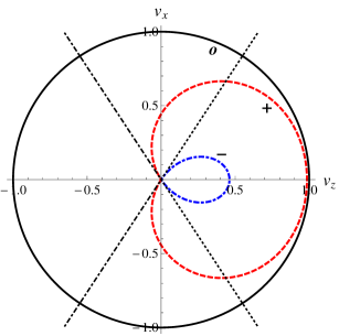
Figure 1: (color online). Normal surfaces for the nonlinear theory described by Eq. (23). The ordinary wave is represented by the circular thick line and the extraordinary waves are represented by the dashed and dot-dashed curves. The symbols $+$, and $-$ and $o$ indicate the solutions presented in Eqs. (25) and (24). The chosen values of the electric and magnetic fields are $B=0.1\lambda$ and $E=0.09\lambda$. These values satisfy Eqs. (28) and (29); hence trirefringence is present. Since this is the case, also birefringence and one refraction must take place. The regions where these effects take place are related to the critical angle, $\theta_{c}$, as given by Eq. (27). The trirefringent region lies between the dotted straight lines, while the birefringent regions are constituted by the angles limited by the dotted and dot-dashed straight lines. The region presenting one refraction lies between the dot-dashed straight lines.

In Fig. 1, the normal surfaces Landau ; born associated with Eqs. (24) and (25) are plotted for a selected set of the fields. It can easily be seen there the region exhibiting trirefringence, as anticipated, for fields satisfying Eqs. (28) and (29).

IV.2 Polarization

Let us now return to the Fresnel-like eigenvalue Eq. (10). The matrix $Z^{\mu}{}_{\nu}$ given by Eq. (11) reduces, for the Lagrangian in Eq. (23), to

$$\frac{Z^{\mu}{}_{\nu}}{q^{2}} = (v^{2}-1)\delta^{\mu}_{\nu}+\frac{4}{F\left(1+\log\frac{F}{\lambda^{2}}\right)}\left[vE^{\mu}+(\hat{q}\cdot\vec{E})V^{\mu}\right.$$ (30)

$$\left.+(\hat{q}\times\vec{B})^{\mu}\right]\left[vE_{\nu}+(\hat{q}\cdot\vec{E})V_{\nu}+(\hat{q}\times\vec{B})_{\nu}\right].$$

This suggests that the polarization vector $\epsilon^{\nu}$ should conveniently be decomposed as a linear combination of the three vectors which appear in $Z^{\mu}{}_{\nu}$ as

$$\epsilon^{\nu}=avE^{\nu}+b(\hat{q}\cdot\vec{E})V^{\nu}+c(\hat{q}\times\vec{B})^{\nu}+dk^{\nu},$$ (31)

where $a,b,c$ are arbitrary constants with the same physical dimension. The fourth term, with an arbitrary constant $d$, was introduced because Eq. (9) remains unchanged by it. Equation (10) then reads

$$[a(v^{2}-1)-Y]vE^{\mu}+[b(v^{2}-1)-Y](\hat{q}\cdot\vec{E})V^{\mu}$$

$$+[c(v^{2}-1)-Y](\hat{q}\times\vec{B})^{\mu}=0,$$ (32)

where $Y$ is a shortcut for

$$Y \doteq \frac{4}{F\left(1+\log\frac{F}{\lambda^{2}}\right)}\left[av^{2}E^{2}-(a+c)v\hat{q}\cdot(\vec{E}\times\vec{B})\right.$$ (33)

$$\left.+c(\hat{q}\times\vec{B})^{2}-b(\hat{q}\cdot\vec{E})^{2}\right].$$

For the $v^{2}=1$ case, Eq. (32) yields $Y=0$, from which the polarization state is given by $a=(\hat{q}\cdot\vec{E})^{2},\;b=E^{2}-(\hat{q}\times\vec{B})^{2},\;c=-(\hat{q}\cdot\vec{E})^{2}$ up to a global multiplicative factor. For the $v^{2}\neq 1$ case, Eq. (32) yields $a=b=c=1$ up to a global multiplicative factor. Assuming $\vec{E}\cdot\vec{B}=0$ and $\hat{q}\cdot\vec{B}=0$, then the phase velocities for this case are given by Eq. (25). Once the physical parameters $a,b,c$ were found in either case, then the particular gauge choice $d=-b(\hat{q}\cdot\vec{E})/(qv)$ ensures $\epsilon^{\nu}$ to lie in the space orthogonal to $V^{\nu}$.

IV.3 Group velocity

It is well known that, in the geometrical optics approximation the wave equation is a linear equation for the perturbed fields, even in the context of nonlinear electrodynamics Birula . In this case wave packets can be build up by superposing plane wave solutions, whose phase velocities were obtained above. Thus, it is important to deal with the group velocities $\vec{u}\doteq{\rm d}\omega/{\rm d}\vec{q}$ for the propagation analysis Landau . For the particular case of the nonlinear Lagrangian density $L_{NL}$, with the same configuration of fields and wave vectors we assumed above, the associated group velocities are

$$\vec{u}=u_{x}\hat{x}+u_{z}\hat{z},$$ (34)

where $u_{x}=\sin\theta$ and $u_{z}=\cos\theta$ for the ordinary $v=1$ mode, thus stating that the group and phase velocities coincide for this case. For the extraordinary modes, we obtain

$$u_{x}^{\pm}=\frac{\chi v_{\pm}^{2}-4EBv_{\pm}\,\cos\theta+2E^{2}\cos^{2}\theta}{\chi v_{\pm}-2EB\,\cos\theta}\,\sin\theta,$$ (35)

and

$$u_{z}^{\pm}=\frac{\chi v_{\pm}^{2}\,\cos\theta-2EBv_{\pm}\cos 2\theta-2E^{2}\cos\theta\,\sin^{2}\theta}{\chi v_{\pm}-2EB\,\cos\theta},$$ (36)

where we are considering $v_{\pm}$ as given by Eq. (25). Hence, two extraordinary rays and one ordinary ray can be found in the $xz$- plane. But their dependence on direction must be investigated more carefully, as we shall do in what follows. If one defines $\varphi$ as the angle between the group velocity and the $z$-axis, then $\varphi=\theta$ for the $v=1$ case. For the extraordinary modes, it follows from Eqs. (35)–(36) that

$$\tan\varphi=\frac{(\chi v_{\pm}^{2}-4EBv_{\pm}\cos\theta+2E^{2}\cos^{2}\theta)\sin\theta}{\chi v_{\pm}^{2}\,\cos\theta-2EBv_{\pm}\cos 2\theta-2E^{2}\cos\theta\,\sin^{2}\theta},$$ (37)

which gives us $\varphi$ as a function of $\theta$. For the case of the extraordinary solutions, the analytical inversion of Eq. (37) to give $\theta$ as a function of $\varphi$ is very involved. Hence, numerical analyses turns out to be more clarifying. Fig. 2 summarizes such a numerical analysis for the same parameters assumed in Fig. 1.

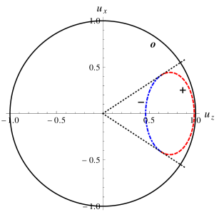
Figure 2: (color online). Ray velocities for the nonlinear model described by Eq. (23). The fields are the same as in Fig. 1. The symbols $+$, $-$ and $o$ indicate the solutions presented in Eqs. (25) and (24) when substituted in Eqs. (34)–(36). As it can be seen, trirefringence occurs in the region lying between the dotted straight lines. In the complementary region only the isotropic ray solution propagates.

One notices that the region of the $xz$ plane where the ordinary and extraordinary group velocities can be found constitutes a trirefringent region. For the complementary region of the plane of propagation, there exists just the ordinary group velocity.

Comparing Figs. 1 and 2 we find angular sectors for which plane waves associated with the extraordinary polarization modes are supposed to propagate, but with no propagation of the corresponding wave packets. This feature relies on the fact that, in our analysis, the wave packets for the extraordinary modes do propagate along directions which are not generally equal to the directions of the corresponding plane waves components, as it is explicitly shown in Eq. (37). This is due to the fact that the phase velocity is dependent upon the direction of the wave vector; hence $\omega=v(\hat{q})q$. This dependence leads to a term in the group velocity that is perpendicular to the phase velocity. The magnitude of such a term may be comparable to the magnitude of the phase velocity itself, yielding therefore to a possibly different behavior of the two aforementioned velocities.

V Conclusion and Discussion

Trirefringence phenomena is not an effect exclusively occurring in nonlinear metamaterials tri1 ; delorenci2012 . As shown here, it is possible to formulate a nonlinear model describing electromagnetism where this effect is also expected to occur. Possible extensions of the presented model can be sought by adding the dual invariant $G$, or else trying other nonlinear Lagrangian models.

As it is well known, in the regime of small fields QED is governed by the Euler-Heisenberg effective Lagrangian density schwinger1951 . In this situation birefringence effect is predicted to occur Birula . Experiments are still under consideration in order to confirm such prediction battesti2008 ; valle2010 . However, when the regime of large fields is considered, the effective Lagrangian governing QED presents the same form as the nonlinear model stated in Eq. (23), leading to the conclusion that trirefringence phenomenon is expected to occur in this regime.

Multirefringence phenomena could also be found for systems described by nonlinear Lagrangian densities which depend on non-Abelian gauge fields. In such cases, the field strength tensors would not be gauge-invariant. Nevertheless, it can be easily shown that the propagation of the field disturbances would be described by the same equations presented above, since only second-order derivatives of the gauge vector field may present non-zero Hadamard discontinuities.

The nonlinear model discussed in the text was proposed long ago savvidy1977 ; pagels1978 ; nielsen1979 as the effective Lagrangian of quantum-chromodynamics (QCD) or other Yang-Mills theories with non-trivial vacuum properties. When considered for this purpose, the Lorentz invariant parameter $F$ in $L(F)$ is extrapolated to be $F^{\mu\nu(a)}F_{\mu\nu(a)}$, where the index $(a)$ runs in the inner Non-Abelian group space. Considering the regime of small coupling and taking the limit of large mean fields ($F/\lambda^{2}\gg 1$) a Lagrangian density with the same functional form as appearing in Eq. (23) is obtained pagels1978 . In this context $b_{0}$ may be identified as a $\beta$-function coefficient at leading order and $\lambda$ a constant related to the mass scale. It was claimed adler1981 that the form for $L_{NL}$ may also result in the leading terms in the limit of weak fields ($F/\lambda^{2}\ll 1$), as in both cases $|\log(F/\lambda^{2})|\gg 1$. Hence trirefringence of non-Abelian gauge fields can also occur and in principle it can be observed, provided the required field configuration is approached. The practical arena for such kind of study is a quark-gluon plasma (QGP), recently observed in high-energy heavy ion collision experiments where the gluon field is deconfined and can propagate in the bulk of the QGP. Some symmetric field configuration has been investigated, and a possible observable has been proposed shi2008 . With the progress of measurements on asymmetries in the experiments, which is now a hot topic in RHIC and LHC, other kind of field configurations can be further investigated.

- (1) Z. Bialynicka-Birula and I. Bialynicki-Birula, Phys. Rev. D 2, 2341 (1970).
- (2) S.L. Adler, Ann. Phys. 67, 599 (1971).
- (3) V.A. De Lorenci, R. Klippert, M. Novello, and J.M. Salim, Phys. Lett. B 482, 134 (2000).
- (4) M. Novello, V.A. De Lorenci, J.M. Salim, and R. Klippert, Phys. Rev. D 61, 045001 (2000).
- (5) E. Iacopini and E. Zavattini, Phys. Lett. B 85, 151 (1979).
- (6) F. Della Valle, G. Di Domenico, U. Gastaldi, E. Milotti, R. Pengo, G. Ruoso, and G. Zavattini, Opt. Commun. 283, 4194 (2010).
- (7) J.I. Latorre, P. Pascual, and R. Tarrach, Nucl. Phys. B 437, 60 (1995).
- (8) I.T. Drummond and S.J. Hathrell, Phys. Rev. D 22, 343 (1980).
- (9) G.M. Shore, Nucl. Phys. B 460, 379 (1996); R.D. Daniels and G.M. Shore, Nucl. Phys. B 425, 634 (1994).
- (10) K. Scharnhorst, Phys. Lett. B 236, 354 (1990).
- (11) G. Barton, Phys. Lett. B 237, 559 (1990).
- (12) W. Dittrich and H. Gies, Phys. Rev. D 58, 025004 (1998); Phys. Lett. B 431, 420 (1998).
- (13) V.A. De Lorenci and S.Y. Li, Phys. Rev. D 78, 034004 (2008).
- (14) L. D. Landau and E. M. Lifshitz, Electrodymanics of Continuous Media, (Pergamon Press, New York, 1984).
- (15) M. Born and E. Wolf, Principles of Optics (Cambridge University Press, Cambridge, England, 1999).
- (16) V.A. De Lorenci and G.P. Goulart, Phys. Rev. D 78, 045015 (2008).
- (17) V.A. De Lorenci, R. Klippert, and D.H. Teodoro, Phys. Rev. D 70, 124035 (2004).
- (18) R. Paschotta, Encyclopedia of laser physics and technology (Wiley-VCH, Weinheim, 2008).
- (19) L. Liu, J.R. Trimarchi, R. Oldenbourg, and D. L. Keefe, Biol. Reprod. 63, 251 (2000); Y. Lim, M. Yamanari, S. Fukuda, Y. Kaji, T. Kiuchi, M. Miura, T. Oshika, and L. Yuasuno, Biomed. Opt. Express 2, 2392 (2011).
- (20) G.D. Fleishman, Q.J. Fu, M. Wang, G.L. Huang, and V.F. Melnikov, Phys. Rev. Lett., 88, 251101 (2002); H.J.M. Cuesta, J.A. de Freitas Pacheco, and J.M. Salim, Int. J. Mod. Phys. A, 21, 43 (2006).
- (21) L. Pagano, P. de Bernardis, G. De Troia, G. Gubitosi, S. Masi, A. Melchiorri, P. Natoli, F. Piacentini, and G. Polenta, Phys. Rev. D, 80, 043522 (2009).
- (22) M.C. Netti, A. Harris, J. Baumberg, D. Whittaker, M. Charlton, M. Zoorob, and G. Parker, Phys. Rev. Lett. 86, 1526 (2001).
- (23) J.D. Joannopoulos, S.G. Johnson, J.N. Winn, and R.D. Meade, Photonic Crystals: Molding the flow of light, (Princeton University Press, Princeton, NJ, 2008), 2nd ed.
- (24) V.A. De Lorenci and J.P. Pereira, Phys. Rev. A 86, 013801 (2012).
- (25) D.R. Smith and D. Schurig, Phys. Rev. Lett. 90, 077405 (2003).
- (26) D.R. Smith, W.J. Padilla, D.C. Vier, S.C. Nemat-Nasser, and S. Schultz, Phys. Rev. Lett. 84, 4184 (2000).
- (27) V.G. Veselago, Sov. Phys. Usp. 10, 509 (1968).
- (28) R.A. Shelby, D.R. Smith, and S. Schultz, Science 292, 77 (2001).
- (29) J. Hadamard, in Leçons sur la propagation des ondes et les équations de l’hydrodynamique (Ed. Hermann, Paris, 1903); G. Boillat, J. Math. Phys. (N.Y.) 11, 941 (1970); A. Papapetrou, in Lectures on General Relativity (Springer, Dordrecht, Holland, 1974).
- (30) W.-Y. Tsai and T. Erber, Phys. Rev. D 10, 492 (1974).
- (31) W.-Y. Tsai, Phys. Rev. D 10, 2699 (1974).
- (32) W.-Y. Tsai and T. Erber, Acta Phys. Austriaca 45, 245 (1976).
- (33) J. Schwinger, Phys. Rev. 82, 664 (1951).
- (34) V. Weisskopf, K. Dan. Vidensk. Selsk. Mat. Fys. Medd. 14, N. 6 (1936).
- (35) J. Schwinger, Phys. Rev. 93, 615 (1954).
- (36) J. Schwinger, Phys. Rev. 94, 1362 (1954).
- (37) P. Elmfors, D. Persson, and B.-S. Skagerstam, Phys. Rev. Lett. 71, 480 (1993).
- (38) H. Pagels and E. Tomboulis, Nucl. Phys. B 143, 485 (1978).
- (39) R. Battesti et al., Eur. Phys. J. D 46, 323 (2008).
- (40) G.K. Savvidy, Phys. Lett. B 71, 133 (1977).
- (41) H.B. Nielsen and M. Ninomiya, Nucl. Phys. B 156, 1 (1979).
- (42) S.L. Adler, in Proceedings of the Fifth John Hopkins Workshop on Current Problems in High Energy Theory, edited by G. Domokos and S. Kövesi-Domokos (Johns Hopkins University, Baltimore, 1981), p. 43.