Simulation of BSDEs with jumps by Wiener Chaos Expansion

Abstract

We present an algorithm to solve BSDEs with jumps based on Wiener Chaos Expansion and Picard’s iterations. This paper extends the results given in [7] to the case of BSDEs with jumps. We get a forward scheme where the conditional expectations are easily computed thanks to chaos decomposition formulas. Concerning the error, we derive explicit bounds with respect to the number of chaos, the discretization time step and the number of Monte Carlo simulations. We also present numerical experiments. We obtain very encouraging results in terms of speed and accuracy.

1 Introduction

In this paper we are interested in the numerical approximation of solutions $(Y,Z,U)$ to backward stochastic differential equations (BSDEs in the sequel) with jumps of the following form

$$Y_{t}=\xi+\int_{t}^{T}f(s,Y_{s},Z_{s},U_{s})\,ds-\int_{t}^{T}Z_{s}dB_{s}-\int_{]t,T]}U_{s}d\tilde{N}_{s},\quad 0\leq t\leq T,$$ (1)

where $B$ is a $1$-dimensional standard Brownian motion and $\tilde{N}$ is a compensated Poisson process independent from B, i.e. $\tilde{N}_{t}:=N_{t}-\kappa t$ and $\{N_{t}\}_{t\geq 0}$ is a Poisson process with intensity $\kappa>0.$ The terminal condition $\xi$ is a real-valued $\mathcal{F}_{T}$–measurable random variable where $\{\mathcal{F}_{t}\}_{0\leq t\leq T}$ stands for the augmented natural filtration associated with $B$ and $N$. Under standard Lipschitz assumptions on the driver $f$, the existence and uniqueness of the solution have been stated by Tang and Li [23], generalizing the seminal paper of Pardoux and Peng [18].

The main objective of this paper is to propose a numerical method to approximate the solution $(Y,Z,U)$ of (1). In the no-jump case, there exist several methods to simulate $(Y,Z)$. The most popular one is the method based on the dynamic programming equation, introduced by Briand, Delyon and Mémin [6]. In the Markovian case, the rate of convergence of the method has been studied by Zhang [24] and Bouchard and Touzi [4]. From a numerical point of view, the main difficulty in solving BSDEs is to compute conditional expectations. Different approaches have been proposed: Malliavin calculus [4], regression methods [10] and quantization techniques [2]. In the general case (i.e. for a terminal condition which is not necessarily Markovian), Briand and Labart [7] have proposed a forward scheme based on Wiener chaos expansion and Picard’s iterations. Thanks to the chaos decomposition formulas, conditional expectations are easily computed, which leads to an efficient, fully implementable scheme. In case of BSDEs driven by a Poisson random measure, Bouchard and Elie [3] have proposed a scheme based on the dynamic programming equation and studied the rate of convergence of the method when the terminal condition is given by $\xi=g(X_{T})$, where $g$ is a Lipschitz function and $X$ is a forward process. More recently, Geiss and Steinicke [9] have extended this result to the case of a terminal condition which may be a Borel function of finitely many increments of the Lévy forward process $X$ which is not necessarily Lipschitz but only satisfies a fractional smoothness condition. In the case of jumps driven by a compensated Poisson process, Lejay, Mordecki and Torres [15] have developed a fully implementable scheme based on a random binomial tree, following the approach proposed by Briand, Delyon and Mémin [5].

In this paper, we extend the algorithm based on Picard’s iterations and Wiener chaos expansion introduced in [7] to the case of BSDEs with jumps. Our starting point is the use of Picard’s iterations: $(Y^{0},Z^{0},U^{0})=(0,0,0)$ and for $q\in\mathbb{N}$,

$$Y^{q+1}_{t}=\xi+\int_{t}^{T}f\left(s,Y^{q}_{s},Z^{q}_{s},U^{q}_{s}\right)ds-\int_{t}^{T}Z^{q+1}_{s}\cdot dB_{s}-\int_{]t,T]}U^{q+1}_{s}d\tilde{N}_{s},\quad 0\leq t\leq T.$$

Writing this Picard scheme in a forward way gives

$$Y^{q+1}_{t} =\mathbb{E}\left(\xi+\int_{0}^{T}f\left(s,Y^{q}_{s},Z^{q}_{s},U^{q}_{s}\right)ds\>\Big{|}\>\mathcal{F}_{t}\right)-\int_{0}^{t}f\left(s,Y^{q}_{s},Z^{q}_{s},U^{q}_{s}\right)ds,$$

$$Z^{q+1}_{t} =\mathbb{E}\left(D^{(0)}_{t}Y^{q+1}_{t}\>\Big{|}\>\mathcal{F}_{t^{-}}\right)=\mathbb{E}\left(D^{(0)}_{t}\left(\xi+\int_{0}^{T}f\left(s,Y^{q}_{s},Z^{q}_{s},U^{q}_{s}\right)ds\right)\>\Big{|}\>\mathcal{F}_{t^{-}}\right),$$

$$U^{q+1}_{t} =\mathbb{E}\left(D^{(1)}_{t}Y^{q+1}_{t}\>\Big{|}\>\mathcal{F}_{t^{-}}\right)=\mathbb{E}\left(D^{(1)}_{t}\left(\xi+\int_{0}^{T}f\left(s,Y^{q}_{s},Z^{q}_{s},U^{q}_{s}\right)ds\right)\>\Big{|}\>\mathcal{F}_{t^{-}}\right),$$

where $D^{(0)}_{t}X$ (resp. $D^{(1)}_{t}X$) stands for the Malliavin derivative of the random variable $X$ with respect to the Brownian motion (resp. w.r.t. the Poisson process).

In order to compute the previous conditional expectation, we use a Wiener chaos expansion of the random variable

$$F^{q}=\xi+\int_{0}^{T}f\left(s,Y^{q}_{s},Z^{q}_{s},U^{q}_{s}\right)ds.$$

More precisely, we use the following orthogonal decomposition of the random variable $F^{q}$ (see Proposition 2.8)

$$F^{q}=\mathbb{E}\left[F^{q}\right]+\sum_{k=1}^{\infty}\sum_{l=0}^{k}\,\sum_{{\bf k}_{l}\in\mathbb{N}^{l}}\,\,\sum_{{\bf j}_{k-l}\in\mathbb{N}^{k-l}}d_{{\bf k}_{l},\,{\bf j}_{k-l}}L^{0,...,0}_{l}(\tilde{e}[k_{1},\ldots,k_{l}])\,L^{1,...,1}_{k-l}(\tilde{e}[j_{1},\ldots,j_{k-l}]).$$

where $L^{0,\cdots,0}_{m}(g)$ (resp. $L^{1,\cdots,1}_{m}(g)$) denotes the iterated integral of order $m$ of $g$ w.r.t. the Brownian motion (resp. w.r.t. the compensated Poisson process), $(\tilde{e}[k_{1},\ldots,k_{m}])_{k_{m}\in\mathbb{N}}$ is an orthogonal basis of $(\tilde{L}^{2})^{\otimes m}([0,T])$, the subspace of symmetric functions from $(L^{2})^{\otimes m}([0,T])$. The sequence of coefficients $\{d_{{\bf k}_{l},\,{\bf j}_{k-l}}\}_{{\bf k}_{l}\in\mathbb{N}^{l},\,{\bf j}_{k-l}\in\mathbb{N}^{k-l}}$ ensues from the Wiener chaos decomposition of $F^{q}$.

The point to get an implementable scheme is that we only keep a finite number of terms in this expansion: we use a finite number of chaos and we choose a finite number of functions $\{e_{1},\cdots,e_{N}\}$ to build $\{\tilde{e}[k_{1},\cdots,k_{m}]\}_{k_{m}\in\{1,\cdots,N\}}$. More precisely, if we choose $e_{i}:=\frac{1}{\sqrt{h}}\mathbf{1}_{]\overline{t}_{i-1},\overline{t}_{i}]}$ where $\overline{t}_{i}=ih$ and $h:=\frac{T}{N}$, we obtain

$$F^{q}\sim\mathbb{E}\left[F^{q}\right]+\sum_{k=1}^{p}\sum_{|n|=k}d^{n}_{k}\prod_{i=1}^{N}K_{n^{B}_{i}}\left(\frac{B_{\overline{t}_{i}}-B_{\overline{t}_{i-1}}}{\sqrt{h}}\right)C_{n^{P}_{i}}(N_{\overline{t}_{i}}-N_{\overline{t}_{i-1}},\kappa h),$$

where $K_{i}$ (resp. $C_{i}$) denotes the Hermite (resp. Charlier) polynomial of degree $i$, $n=(n^{B}_{1},\cdots,n^{B}_{N},n^{P}_{1},$ $\cdots,n^{P}_{N})$ is a vector of integers and $|n|=\sum_{i=1}^{N}(n^{B}_{i}+n^{P}_{i})$. By using this approximation of $F^{q}$ we can easily compute $\mathbb{E}(F^{q}|\mathcal{F}_{t})$, $\mathbb{E}(D^{(0)}_{t}F^{q}|\mathcal{F}_{t^{-}})$ and $\mathbb{E}(D^{(1)}_{t}F^{q}|\mathcal{F}_{t^{-}})$, which gives us $(Y^{q+1}_{t},Z^{q+1}_{t},U^{q+1}_{t})$. To get a fully implementable algorithm, it remains to approximate $\mathbb{E}(F^{q})$ and the coefficients $\{d^{n}_{k}\}_{n,k}$ by Monte Carlo.

When extending [7] to the jump case one realizes that the main difficulty lies in the fact that there is no hypercontractivity property in the Poisson chaos decomposition case. This property plays an important role in the proof of the convergence in the Brownian case. To circumvent this problem, we exploit a recent result of Last, Penrose, Schulte and Thäle [13], which gives a formula to compute the expectation of products of Poisson multiple integrals, and the according result for the Brownian case from Peccati and Taqqu [19]. In fact, in equation (20) of Proposition 2.11 we get an explicit expression for

$$\mathbb{E}(I_{n_{1}}(f_{n_{1}})\cdots I_{n_{l}}(f_{n_{l}}))$$

in terms of a combinatoric sum of tensor products of the chaos kernels $f_{n_{i}}.$ Here $I_{n_{i}}(f_{n_{i}})$ denotes the multiple integral of order $n_{i}$ with respect to the process $B+\tilde{N}.$ By this expression one gets the required estimates for the truncated chaos without the hypercontractivity property. Therefore, to prove the convergence of the method we may proceed similarly to [7], and split the error into four terms:

• the error due to Picard iterations

• the error due to the truncation onto the chaos up to order $p$

• the error due to the finite number of basis functions $\{e_{1},\cdots,e_{N}\}$ for each chaos

• the error due to the Monte Carlo simulations to approximate the expectations appearing in the coefficients $\{d^{n}_{k}\}_{n,k}.$

The paper is organized as follows: Section 2 contains the notations and gives preliminary results, Section 3 describes the approximation procedure, Section 4 states the convergence results and Section 5 presents the algorithm and some numerical examples. Some technical results are proved in the appendix.

1.1 Definitions and Notations

Given a probability space $(\Omega,\mathcal{F},\mathbb{P})$ we consider

• $\mathrm{L}^{p}(\mathcal{F}_{T}):=\mathrm{L}^{p}(\Omega,\mathcal{F}_{T},\mathbb{P})$, $p\in\mathbb{N}^{*}=\mathbb{N}\setminus\{0\}$, the space of all $\mathcal{F}_{T}$-measurable random variables (r.v. in the following) $X:\Omega\longmapsto\mathbb{R}$ satisfying $\|X\|^{p}_{p}:=\mathbb{E}(|X|^{p})<\infty$.

• $\mathrm{S}^{p}_{T}(\mathbb{R})$, $p\in\mathbb{N},p\geq 2$, the space of all càdlàg, adapted processes $\phi:\Omega\times[0,T]\longmapsto\mathbb{R}$ such that $\|\phi\|^{p}_{\mathrm{S}^{p}}=\mathbb{E}(\sup_{t\in[0,T]}|\phi_{t}|^{p})<\infty$.

• $\mathrm{H}^{p}_{T}(\mathbb{R})$, $p\in\mathbb{N},p\geq 2$, the space of all predictable processes $\phi:\Omega\times[0,T]\longmapsto\mathbb{R}$ such that $\|\phi\|^{p}_{\mathrm{H}^{p}_{T}}=\mathbb{E}(\int_{0}^{T}|\phi_{t}|^{p}dt)<\infty$.

• $\mathrm{L}^{2}(0,T)$, the space of all square integrable functions on $[0,T]$.

• $C^{k,l}$, the set of continuously differentiable functions $\phi:(t,x)\in[0,T]\times\mathbb{R}^{3}$ with continuous derivatives w.r.t. $t$ (resp. w.r.t. $x$) up to order $k$ (resp. up to order $l$).

• $C^{k,l}_{b}$, the set of continuously differentiable functions $\phi:(t,x)\in[0,T]\times\mathbb{R}^{3}$ with continuous and uniformly bounded derivatives w.r.t. $t$ (resp. w.r.t. $x$) up to order $k$ (resp. up to order $l$). The function $\phi$ is also bounded.

• $\|\partial^{j}_{sp}f\|^{2}_{\infty}$, the sum of the squared norms of the derivatives of $f([0,T]\times\mathbb{R}^{3},\mathbb{R})$ w.r.t. all the space variables $x$ which sum equals $j$ : $\|\partial^{j}_{sp}f\|^{2}_{\infty}:=\sum_{|k|=j}\|\partial^{k_{1}}_{x_{1}}\partial^{k_{2}}_{x_{2}}\partial^{k_{3}}_{x_{3}}f\|^{2}_{\infty}$, where $|k|=k_{1}+k_{2}+k_{3}$.

• $C^{\infty}_{p}$, the set of smooth functions $f:\mathbb{R}^{n}\longmapsto\mathbb{R}$ ($n\geq 1$) with partial derivatives of polynomial growth.

• $\|(\cdot,\cdot,\cdot)\|^{p}_{\mathrm{L}^{p}}$, $p\geq 1$, the norm on the space $\mathrm{S}^{p}_{T}(\mathbb{R})\times\mathrm{H}^{p}_{T}(\mathbb{R})\times\mathrm{H}^{p}_{T}(\mathbb{R})$ defined by

  $$\|(Y,Z,U)\|^{p}_{\mathrm{L}^{p}}:=\mathbb{E}(\sup_{t\in[0,T]}|Y_{t}|^{p})+\int_{0}^{T}\mathbb{E}(|Z_{t}|^{p})dt+\kappa\int_{0}^{T}\mathbb{E}(|U_{t}|^{p})dt.$$ (2)

Hypothesis 1.1.

We assume

• the terminal condition $\xi$ belongs to $\mathrm{L}^{2}(\mathcal{F}_{T})$;

• the generator $f\in C([0,T]\times\mathbb{R}^{3};\mathbb{R})$ is Lipschitz continuous in space, uniformly in $t$: there exists a constant $L_{f}$ such that

  $$|f(t,y_{1},z_{1},u_{1})-f(t,y_{2},z_{2},u_{2})|\leq L_{f}\left(|y_{1}-y_{2}|+|z_{1}-z_{2}|+|u_{1}-u_{2}|\right).$$

Lemma 1.2.

If Hypothesis 1.1 is satisfied and $\xi\in\mathbb{D}^{1,2}$ (defined below) we get from [9, Theorem 3.4] that for a.e. $t\in[0,T]$

$$Z_{t}=\mathbb{E}[D^{(0)}_{t}Y_{t}|\mathcal{F}_{t-}],\quad U_{t}=\mathbb{E}[D^{(1)}_{t}Y_{t}|\mathcal{F}_{t-}]\,\,\,\,\mathbb{P}-{\mbox{a}.s.}$$ (3)

where $D^{(0)}_{t}X$ stands for the Malliavin derivative w.r.t. the Brownian motion of the random variable $X$, and $D^{(1)}_{t}X$ stands for the Malliavin derivative w.r.t. the Poisson process of the random variable $X$. Here $\mathbb{E}[\cdot|\mathcal{F}_{t-}]$ should be understood as the predictable projection, and since the paths $s\mapsto D^{(i)}_{t}Y_{s}$ are a.s. càdlàg we define $D^{(i)}_{t}Y_{t}:=\lim_{s\downarrow t}D^{(i)}_{t}Y_{s}$ if the limit exists, and zero otherwise.

2 Wiener Chaos Expansion

2.1 Notations and useful results

2.1.1 Iterated integrals

We refer to [16] and [21] for more details on this section. Let us briefly recall the Wiener chaos expansion in the case of a real-valued Brownian motion and an independent Poisson process with intensity $\kappa>0.$

We define

$$G_{0}(t)=B_{t},\quad G_{1}(t)=N_{t}-\kappa t,$$

and $L_{k}^{i_{1},\cdots,i_{k}}(f)$ the iterated integral of $f$ with respect to $G_{0}$ and $G_{1}$

$$L_{k}^{i_{1},\cdots,i_{k}}(f)=\int_{0}^{T}\left(\int_{0}^{t_{k}^{-}}\cdots\left(\int_{0}^{t_{2}^{-}}f(t_{1},\ldots,t_{k})dG_{i_{1}}(t_{1})\right)\cdots dG_{i_{k-1}}(t_{k-1})\right)dG_{i_{k}}(t_{k}).$$

We have the following chaotic representation property.

Proposition 2.3.

([16, Proposition 2.1]) For $k\in\mathbb{N}^{*}$ define

$$\mathbf{i}_{k}:=(i_{1},\ldots,i_{k})\in\{0,1\}^{k}.$$

Any $F\in\mathrm{L}^{2}(\mathcal{F}_{T})$ has a unique representation of the form

$$F=\mathbb{E}(F)+\sum_{k=1}^{\infty}\,\,\sum_{\mathbf{i}_{k}\in\{0,1\}^{k}}L_{k}^{{\mathbf{i}_{k}}}(f_{\mathbf{i}_{k}}),$$ (4)

where $f_{\mathbf{i}_{k}}\in L^{2}(\Sigma_{k})$ and $\Sigma_{k}=\{(t_{1},\ldots,t_{k})\in[0,T]^{k}:0<t_{1}<\cdots<t_{k}<T\}$ is the simplex of $[0,T]^{k}$.

Let $|\mathbf{i}_{k}|:=\sum_{j=1}^{k}i_{j}$. Due to the isometry property it holds

$$\|L_{k}^{\mathbf{i}_{k}}(f)\|^{2}=\kappa^{|\mathbf{i}_{k}|}\|f\|^{2}_{\Sigma_{k}},$$

and for any $f\in L^{2}(\Sigma_{k}),$ $g\in L^{2}(\Sigma_{m})$, $\mathbf{i}_{k}\in\{0,1\}^{k}$, and $\mathbf{j}_{m}\in\{0,1\}^{m}$ we have (see [16, Proposition 1.1])

$$\mathbb{E}[L_{k}^{\mathbf{i}_{k}}(f)L_{m}^{\mathbf{j}_{m}}(g)]=\left\{\begin{array}[]{cc}\kappa^{|\mathbf{i}_{k}|}\int_{\Sigma_{k}}f(t_{1},\cdots,t_{k})g(t_{1},\cdots,t_{k})dt_{1}\cdots dt_{k}&\mbox{ if $\mathbf{i}_{k}=\mathbf{j}_{m}$}\\ 0&\mbox{ otherwise.}\\ \end{array}\right.$$

Then, $\|F\|^{2}=\mathbb{E}[F]^{2}+\sum_{k\geq 1}\sum_{\mathbf{i}_{k}}\kappa^{|\mathbf{i}_{k}|}\|f_{\mathbf{i}_{k}}\|^{2}_{L^{2}(\Sigma_{k})}$. The chaos approximation of $F$ up to order $p$ is defined by

$$\mathcal{C}_{p}(F) :=\mathbb{E}(F)+\sum_{k=1}^{p}\sum_{\mathbf{i}_{k}}L_{k}^{{\mathbf{i}_{k}}}(f_{\mathbf{i}_{k}})$$ (5)

and $P_{k}(F):=\sum_{\mathbf{i}_{k}}L_{k}^{{\mathbf{i}_{k}}}(f_{\mathbf{i}_{k}})$ is the Wiener chaos of order $k$ of $F$. We have

$$\mathbb{E}[(P_{k}(F))^{2}]=\sum_{\mathbf{i}_{k}}\kappa^{|\mathbf{i}_{k}|}\|f_{\mathbf{i}_{k}}\|^{2}_{\Sigma_{k}}.$$ (6)

• Let $f\in L^{2}(\Sigma_{k})$ and $j\in\{0,1\}$. Following [16], we define the derivative of $L_{k}^{\mathbf{i}_{k}}(f)$ w.r.t. the Brownian motion and the Poisson process as the element of $L^{2}(\Omega\times[0,T])$ given by

  $$D^{(j)}_{t}L_{k}^{\mathbf{i}_{k}}(f) =\sum_{l=1}^{k}\mathbf{1}_{\{i_{l}=j\}}L_{k-1}^{i_{1},\cdots,\widehat{i_{l}},\cdots,i_{k}}(f(\underbrace{\cdots}_{l-1},t,\cdots)),$$ (7)

  where $\widehat{i}$ means that the $i$-th index is omitted.

• Let $j\in\{0,1\}.$ We extend the definition of $D^{(j)}$ to

  $$Dom\;D^{(j)}:=\left\{F\in L^{2}(\mathcal{F}_{T})\mbox{ satisfying \eqref{eq0} and }\sum_{k=1}^{\infty}\sum_{\mathbf{i}_{k}}\sum_{l=1}^{k}\mathbf{1}_{\{i_{l}=j\}}\,\kappa^{|\mathbf{i}_{k}|}\|f_{{\mathbf{i}_{k}}}\|^{2}_{\Sigma_{k}}<\infty\right\}.$$

  If $F\in Dom\;D^{(j)}$ then

  $$\|F\|^{2}_{Dom\;D^{(j)}}:=\mathbb{E}|F|^{2}+\kappa^{j}\mathbb{E}\int_{0}^{T}|D^{(j)}_{t}F|^{2}dt<\infty.$$

• $F$ with chaotic representation (4) belongs to $Dom\;D=:\mathbb{D}^{1,2}$ if $F$ belongs to
  $Dom\;D^{(0)}\cap Dom\;D^{(1)}$, i.e.

  $$\|F\|^{2}_{\mathbb{D}^{1,2}}:=\mathbb{E}|F|^{2}+\sum_{k=1}^{\infty}k\sum_{\mathbf{i}_{k}}\kappa^{|\mathbf{i}_{k}|}\|f_{\mathbf{i}_{k}}\|^{2}_{\Sigma_{k}}<\infty.$$

  More generally, we define $\mathbb{D}^{m,2}$ as follows:

• Let $m\geq 1$. We say that $F$ satisfying (4) belongs to $\mathbb{D}^{m,2}$ if it holds

  $$\|F\|^{2}_{\mathbb{D}^{m,2}}:=\mathbb{E}|F|^{2}+\sum_{l=1}^{m}\sum_{k=l}^{\infty}\frac{k!}{(k-l)!}\sum_{\mathbf{i}_{k}}\kappa^{|\mathbf{i}_{k}|}\|f_{\mathbf{i}_{k}}\|^{2}_{\Sigma_{k}}<\infty.$$

  We recall

  $$\mathbb{D}^{\infty,2}=\cap_{m=1}^{\infty}\mathbb{D}^{m,2}.$$

  We define for $l\in\mathbb{N}^{*}$ with $l\leq m$ the seminorm $\|\cdot\|_{D^{l}}$ on $\mathbb{D}^{m,2}$ by

  $$\|F\|^{2}_{D^{l}}:=\sum_{\begin{subarray}{c}\mathbf{i}_{l}\end{subarray}}\kappa^{|\mathbf{i}_{l}|}\mathbb{E}\left(\int_{0}^{T}\cdots\int_{0}^{T}\left|D^{\mathbf{i}_{l}}_{t_{1},\cdots,t_{l}}F\right|^{2}dt_{1}\cdots dt_{l}\right)=\sum_{k=l}^{\infty}\frac{k!}{(k-l)!}\sum_{\mathbf{i}_{k}}\kappa^{|\mathbf{i}_{k}|}\|f_{\mathbf{i}_{k}}\|^{2}_{\Sigma_{k}},$$ (8)

  where $D^{\mathbf{i}_{l}}_{t_{1},\cdots,t_{l}}=D^{i_{1}}_{t_{1}}\cdots D^{i_{l}}_{t_{l}}$ represents the multi-index Malliavin derivative.

  Remark 2.4.

  By using this notation we have $\|F\|^{2}_{\mathbb{D}^{m,2}}=\mathbb{E}|F|^{2}+\sum_{l=1}^{m}\|F\|^{2}_{D^{l}}$.

• For $m\geq 1$ and $j\in\mathbb{N}^{*}$ we define $\mathcal{D}^{m,j}$ as the space of all $F\in\mathbb{D}^{m,2}$ such that

  $$\|F\|^{j}_{m,j}:=\sum_{1\leq l\leq m}\,\sum_{\mathbf{i}_{l}\in\{0,1\}^{l}}\,\,\operatorname*{ess\,sup}_{(t_{1},\cdots,t_{l})\in[0,T]^{l}}\mathbb{E}[|D^{\mathbf{i}_{l}}_{t_{1},\cdots,t_{l}}F|^{j}]<\infty.$$

  (Since $(\omega,t_{1},...,t_{l})\mapsto(D^{\mathbf{i}_{l}}_{t_{1},\cdots,t_{l}}F)(\omega)$ is regarded as an element of $L^{2}(\Omega\times[0,T]^{l})$ w.r.t. the measure $\mathbb{P}\otimes\lambda_{d}$ ($\lambda_{d}$ denotes the Lebesgue measure on $\mathbb{R}^{d}$) we use the essential supremum w.r.t. $\lambda_{d}$.)

• $\mathcal{S}^{m,j}$ denotes the space of all triples of processes $(Y,Z,U)$ belonging to $\mathrm{S}^{j}_{T}(\mathbb{R})\times\mathrm{H}^{j}_{T}(\mathbb{R}^{d})\times\mathrm{H}^{j}_{T}(\mathbb{R})$ and such that

  $$\|(Y,Z,U)\|^{j}_{m,j}: =\sum_{1\leq l\leq m}\sum_{\begin{subarray}{c}\mathbf{i}_{l}\end{subarray}}\operatorname*{ess\,sup}_{(t_{1},\cdots,t_{l})\in[0,T]^{l}}\|(D^{\mathbf{i}_{l}}_{t_{1},\cdots,t_{l}}Y,D^{\mathbf{i}_{l}}_{t_{1},\cdots,t_{l}}Z,D^{\mathbf{i}_{l}}_{t_{1},\cdots,t_{l}}U)\|^{j}_{\mathrm{L}^{j}}<\infty,$$

  where $\|\cdot\|^{j}_{\mathrm{L}^{j}}$ has been defined in (2). We denote $\mathcal{S}^{m,\infty}:=\cap_{j=1}^{\infty}\mathcal{S}^{m,j}$.

Remark 2.5.

If $F:=g(G)$, where $g:\mathbb{R}\rightarrow\mathbb{R}$ is a $\mathcal{C}^{1}_{b}$ function and $G\in\mathbb{D}^{1,2},$ we have (following [8, Proposition 5.1]) that

$$(D_{t}^{(0)}F,D_{t}^{(1)}F)=(g^{\prime}(G)D^{(0)}_{t}G,\,g(G+D_{t}^{(1)}G)-g(G)).$$

Moreover, using Notation (8), we get

$$\|F\|^{2}_{D^{1}}=\|D^{(0)}F\|^{2}_{L^{2}(\Omega\times[0,T])}+\kappa\|D^{(1)}F\|^{2}_{L^{2}(\Omega\times[0,T])}\leq\|g^{\prime}\|^{2}_{\infty}\|G\|^{2}_{D^{1}}.$$

More generally, if $g:\mathbb{R}\rightarrow\mathbb{R}$ is a $\mathcal{C}^{m}_{b}$ function and $G\in\mathbb{D}^{m,2}$, we have

$$\|F\|^{2}_{D^{m}}\leq C(m,\{\|g^{(k)}\|_{\infty}\}_{k\leq m},\|G\|_{\mathbb{D}^{m,2}}),$$

where $C(m,\{\|g^{(k)}\|_{\infty}\}_{k\leq m},\|G\|_{\mathbb{D}^{m,2}}\!)$ is a constant depending on $m,\{\|g^{(k)}\|_{\infty}\!\}_{k\leq m}$ and $\|G\|_{\mathbb{D}^{m,2}}.$

Lemma 2.6.

Let $1\leq m\leq p+1$ and $F\in\mathbb{D}^{m,2}$. We have

$$\mathbb{E}[|F-\mathcal{C}_{p}(F)|^{2}]\leq\frac{\|F\|^{2}_{D^{m}}}{(p+2-m)\cdots(p+1)}.$$

Proof.

Using (6), we get

$$\mathbb{E}[|F-\mathcal{C}_{p}(F)|^{2}] =\sum_{k\geq p+1}\mathbb{E}[P_{k}(F)^{2}]=\sum_{k\geq p+1}\sum_{\mathbf{i}_{k}}\kappa^{|\mathbf{i}_{k}|}\|f_{\mathbf{i}_{k}}\|^{2}_{\Sigma_{k}}$$

$$=\sum_{k\geq p+1}\frac{k!}{(k-m)!}\frac{(k-m)!}{k!}\sum_{\mathbf{i}_{k}}\kappa^{|\mathbf{i}_{k}|}\|f_{\mathbf{i}_{k}}\|^{2}_{\Sigma_{k}}$$

$$\leq\frac{1}{(p+2-m)\cdots(p+1)}\sum_{k\geq p+1}\frac{k!}{(k-m)!}\sum_{\mathbf{i}_{k}}\kappa^{|\mathbf{i}_{k}|}\|f_{\mathbf{i}_{k}}\|^{2}_{\Sigma_{k}}.$$

$$\leq\frac{1}{(p+2-m)\cdots(p+1)}\sum_{k\geq m}\frac{k!}{(k-m)!}\sum_{\mathbf{i}_{k}}\kappa^{|\mathbf{i}_{k}|}\|f_{\mathbf{i}_{k}}\|^{2}_{\Sigma_{k}}.$$

∎

2.1.2 Multiple integrals

In the following, $\lambda$ denotes the Lebesgue measure. Setting

$$M(ds,dx):=dG_{0}(s)d\delta_{0}(x)+dG_{1}(s)d\delta_{1}(x)$$

we get an independent random measure in the sense of Itô (see [11]). There exists a chaotic representation by multiple integrals w.r.t. this random measure $M$ which is equivalent to Proposition 2.3.

Proposition 2.7.

([11]) Any $F\in L^{2}(\mathcal{F}_{T})$ can be represented as

$$F=\mathbb{E}[F]+\sum_{k=1}^{\infty}I_{k}(g_{k}),$$ (9)

with $g_{k}\in(L^{2})^{\otimes k}(\lambda\otimes(\delta_{0}+\kappa\delta_{1})):=(L^{2})^{\otimes k}([0,T]\times\{0,1\},\mathcal{B}([0,T])\otimes 2^{\{0,1\}},\lambda\otimes(\delta_{0}+\kappa\delta_{1}))$. This representation is unique if we assume that the functions $g_{k}(z_{1},...,z_{k})$ with $z_{i}=(t_{i},x_{i})\in[0,T]\times\{0,1\}$ are symmetric.

For the definition of the multiple integrals $I_{k}(g_{k})$ we refer to [11] or [12]. But using the result that the representations in Proposition 2.3 and 2.7 are both unique we conclude for symmetric $g_{k}$ the relation

$$I_{k}(g_{k})=k!\sum_{\mathbf{i}_{k}}L_{k}^{\mathbf{i}_{k}}(g_{k}((\cdot,i_{1}),\cdots,(\cdot,i_{k}))),$$ (10)

where $\mathbf{i}_{k}$ is defined in Proposition 2.3 and

$$g_{k}(((t_{1},i_{1}),\cdots,(t_{k},i_{k})))=k!f_{\mathbf{i}_{k}}(t_{1},\ldots,t_{k})\quad\text{ on }\Sigma_{k}$$

with $f_{\mathbf{i}_{k}}$ from Proposition 2.3.

Moreover, for symmetric $g_{k}\in(L^{2})^{\otimes k}(\lambda\otimes(\delta_{0}+\kappa\delta_{1}))$ and $f_{m}\in(L^{2})^{\otimes m}(\lambda\otimes(\delta_{0}+\kappa\delta_{1}))$ the relation

$$\mathbb{E}[I_{k}(g_{k})I_{m}(f_{m})]=\left\{\begin{array}[]{cc}k!\langle g_{k},f_{k}\rangle_{(L^{2})^{\otimes k}(\lambda\otimes(\delta_{0}+\kappa\delta_{1}))}&\mbox{ if $k=m$}\\ 0&\mbox{ otherwise,}\\ \end{array}\right.$$ (13)

holds true. If $F\in\mathbb{D}^{m,2}$, we combine (9), (10) and [16, Definition 1.7] (which extends (7) to functions defined on $L^{2}([0,T])^{k}$) to get

$$g_{k}((t_{1},i_{1}),\ldots,(t_{k},i_{k}))=\frac{1}{k!}\mathbb{E}D^{\mathbf{i}_{k}}_{t_{1},\ldots,t_{k}}F,\quad k\leq m.$$ (14)

On the other hand, this can be easily derived if one takes into account that for $F=\mathbb{E}[F]+\sum_{k=1}^{\infty}I_{k}(g_{k})$ we have $D^{\mathbf{i}_{1}}_{t_{1}}F=\sum_{k=1}^{\infty}kI_{k-1}(g_{k}((t_{1},i_{1}),\cdot)),$ and that the expectation of any multiple integral of order $k>0$ is zero while $I_{0}$ is the identity map.

For the implementation of the numerical scheme we will use Hermite and Charlier polynomials. In order to do so, we provide a chaotic representation consisting only of iterated integrals of the form $L^{0,...,0}$ and $L^{1,...,1}$ for which the relations (24) and (25) below can be used.

Use $\{p_{0},p_{1}\}=\{\mathbf{1}_{\{0\}},\frac{1}{\sqrt{\kappa}}\mathbf{1}_{\{1\}}\}$ as orthonormal basis of $L^{2}(\{0,1\},2^{\{0,1\}},\delta_{0}+\kappa\delta_{1})$ and fix an orthonormal basis $\{e_{k}\}_{k\in\mathbb{N}}$ for $L^{2}([0,T],\mathcal{B}([0,T]),\lambda)$. By setting

$$e[(k_{1},i_{1}),\ldots,(k_{m},i_{m})]:=(e_{k_{1}}\otimes p_{i_{1}})\otimes\ldots\otimes(e_{k_{m}}\otimes p_{i_{m}}),\quad k_{j}\in\mathbb{N},i_{j}\in\{0,1\}$$

we get an orthonormal basis of $(L^{2})^{\otimes m}(\lambda\otimes(\delta_{0}+\kappa\delta_{1})).$ The symmetrizations

$$\tilde{e}[(k_{1},i_{1}),\ldots,(k_{m},i_{m})]:=\frac{1}{m!}\sum_{\pi\in\mathcal{S}_{m}}e[(k_{\pi(1)},i_{\pi(1)}),\ldots,(k_{\pi(m)},i_{\pi(m)})],\quad k_{j}\in\mathbb{N},i_{j}\in\{0,1\}$$ (15)

form an orthogonal basis of $\tilde{(L^{2})}^{\otimes m}(\lambda\otimes(\delta_{0}+\kappa\delta_{1})),$ the subspace of symmetric functions from $(L^{2})^{\otimes m}(\lambda\otimes(\delta_{0}+\kappa\delta_{1})).$

We also will use the notation

$$\tilde{e}[k_{1},\ldots,k_{m}]:=\frac{1}{m!}\sum_{\pi\in\mathcal{S}_{m}}e_{k_{\pi(1)}}\otimes\cdots\otimes e_{k_{\pi(m)}},\quad k_{j}\in\mathbb{N},$$

where $\mathcal{S}_{m}$ stands for the set of all permutations of $\{1,...,m\}.$

Proposition 2.8.

Any $F\in L^{2}(\mathcal{F}_{T})$ can be represented as

$$F =\mathbb{E}[F]+\sum_{k=1}^{\infty}\sum_{l=0}^{k}\,\sum_{{\bf k}_{l}\in\mathbb{N}^{l}}\,\,\sum_{{\bf j}_{k-l}\in\mathbb{N}^{k-l}}d_{{\bf k}_{l},{\bf j}_{k-l}}L^{0,...,0}_{l}(\tilde{e}[k_{1},\ldots,k_{l}])\,L^{1,...,1}_{k-l}(\tilde{e}[j_{1},\ldots,j_{k-l}]),$$

where $d_{{\bf k}_{l},{\bf j}_{k-l}}=\frac{l!(k-l)!\langle g_{k},e[(k_{1},0),....(k_{l},0)]\otimes e[(j_{1},1),...,(j_{k-l},1)]\rangle_{(L^{2})^{\otimes k}}}{\kappa^{\frac{k-l}{2}}\|\tilde{e}[(k_{1},0),....(k_{l},0),(j_{1},1),...,(j_{k-l},1)]\|^{2}_{(L^{2})^{\otimes k}(\lambda\otimes(\delta_{0}+\kappa\delta_{1}))}}.$

Proof.

According to [11, Theorem 1] a permutation of the coordinates of the kernels does not change the multiple integral, i.e. for any $\pi\in\mathcal{S}_{k}$ we have

$$I_{k}(\tilde{e}[(k_{1},i_{1}),\ldots,(k_{k},i_{k})])=I_{k}(e[(k_{\pi(1)},i_{\pi(1)}),\ldots,(k_{\pi(k)},i_{\pi(k)})]).$$

For any $\pi$ with $(i_{\pi(1)},\ldots,i_{\pi(k)})=(0,\ldots,0,1,\ldots,1)$ (we assume that $(i_{1},\ldots,i_{k})$ contains $l$ zeros) it holds by the product formula for multiple integrals (see A.5 or [14, Theorem 3.6])

$$I_{k}(\tilde{e}[(k_{1},i_{1}),\ldots,(k_{k},i_{k})])=I_{l}(e[(k_{\pi(1)},0),\ldots,(k_{\pi(l)},0)])I_{k-l}(e[(k_{\pi(l+1)},1),\ldots,(k_{\pi(k)},1)])$$ (16)

since

$$e[(k_{\pi(1)},i_{\pi(1)}),\ldots,(k_{\pi(k)},i_{\pi(k)})]=e[(k_{\pi(1)},0),\ldots,(k_{\pi(l)},0)]\otimes e[(k_{\pi(l+1)},1),\ldots,(k_{\pi(k)},1)],$$

and for the contraction-identification $\otimes_{m}^{r}$ (for the definition see (59)) it holds

$$e[(k_{\pi(1)},0),\ldots,(k_{\pi(l)},0)]\otimes_{m}^{r}e[(k_{\pi(l+1)},1),\ldots,(k_{\pi(k)},1)]=0$$

if $r\neq 0$ or $m\neq 0.$ Since

$$e[(k_{\pi(l+1)},1),\ldots,(k_{\pi(k)},1)]=\frac{1}{\kappa^{\frac{k-l}{2}}}e[k_{\pi(l+1)},\ldots,k_{\pi(k)}],$$

we conclude from (16) and (10) that

$$I_{k}(\tilde{e}[(k_{1},i_{1}),\ldots,(k_{k},i_{k})])=\frac{l!(k-l)!}{\kappa^{\frac{k-l}{2}}}L^{0,...,0}_{l}(\tilde{e}[k_{\pi(1)},\ldots,k_{\pi(l)}])L^{1,...,1}_{k-l}(\tilde{e}[k_{\pi(l+1)},\ldots,k_{\pi(k)}]).$$ (17)

The symmetric functions $g_{k}$ from Proposition 2.7 can be written as

$$g_{k}= \sum_{l=0}^{k}\sum_{{\bf k}_{l}}\sum_{{\bf j}_{k-l}}\langle g_{k},e[(k_{1},0),...,(k_{l},0)]\otimes e[(j_{1},1),...,(j_{k-l},1)]\rangle_{(L^{2})^{\otimes k}}$$

$$\quad\quad\quad\quad\quad\quad\times\tilde{e}[(k_{1},0),...,(k_{l},0),(j_{1},1),...,(j_{k-l},1)]c_{{\bf k}_{l},{\bf j}_{k-l}},$$ (18)

where we sum over all ${\bf k}_{l}\in\mathbb{N}^{l}$ and ${\bf j}_{k-l}\in\mathbb{N}^{k-l}$ and

$$c_{{\bf k}_{l},{\bf j}_{k-l}}=\|\tilde{e}[(k_{1},0),...,(k_{l},0),(j_{1},1),...,(j_{k-l},1)]\|^{-2}_{(L^{2})^{\otimes k}(\lambda\otimes(\delta_{0}+\kappa\delta_{1}))}$$

denotes the normalizing factor. Abbreviating

$$d_{{\bf k}_{l},{\bf j}_{k-l}}:=\frac{l!(k-l)!}{\kappa^{\frac{k-l}{2}}}\langle g_{k},e[(k_{1},0),...,(k_{l},0)]\otimes e[(j_{1},1),...,(j_{k-l},1)]\rangle_{(L^{2})^{\otimes k}}\,c_{{\bf k}_{l},{\bf j}_{k-l}}$$

we conclude from Proposition 2.7, (17) and (2.1.2) the orthogonal decomposition

$$F =\mathbb{E}[F]+\sum_{k=1}^{\infty}\sum_{l=0}^{k}\sum_{{\bf k}_{l}}\sum_{{\bf j}_{k-l}}d_{{\bf k}_{l},{\bf j}_{k-l}}L^{0,...,0}_{l}(\tilde{e}[k_{1},\ldots,k_{l}])\,L^{1,...,1}_{k-l}(\tilde{e}[j_{1},\ldots,j_{k-l}]).$$ (19)

∎

Lemma 2.9.

Fix $N\in\mathbb{N}^{*}$ and let

$$e[(k_{1},0),...,(k_{l},0),(j_{1},1),...,(j_{k-l},1)]=\bigotimes_{i=1}^{N}(e_{i}\otimes p_{0})^{\otimes n^{B}_{i}}\otimes\bigotimes_{j=1}^{N}(e_{j}\otimes p_{1})^{\otimes n^{P}_{j}},$$

i.e. $n^{B}_{i}$ and $n^{P}_{i}$ $(1\leq i\leq N)$ denote the multiplicities of the functions $e_{i}\otimes p_{0}$ and $e_{i}\otimes p_{1}$, respectively, so that $|{\bf n}^{B}|=|(n_{1}^{B},...,n_{N}^{B})|=l$ and $|{\bf n}^{P}|=|(n_{1}^{P},...,n_{N}^{P})|=k-l.$ Let ${\bf n}^{A}!:=n^{A}_{1}!\cdots n^{A}_{N}!$ for $A=B,P$ and define ${\bf n}:=({\bf n}^{B},{\bf n}^{P})$ so that $|{\bf n}|=|{\bf n}^{B}|+|{\bf n}^{P}|.$ Then

$$c_{{\bf k}_{l},{\bf j}_{k-l}}=\|\tilde{e}[(k_{1},0),...,(k_{l},0),(j_{1},1),...,(j_{k-l},1)]\|^{-2}_{(L^{2})^{\otimes k}(\lambda\otimes(\delta_{0}+\kappa\delta_{1}))}=\frac{|{\bf n}|!}{{\bf n}^{B}!\,{\bf n}^{P}!}.$$

Proof.

To compute $c_{{\bf k}_{l},{\bf j}_{k-l}}$ notice that the functions $h_{j}:=(e_{k_{j}}\otimes p_{i_{j}})$ and $h_{j^{\prime}}$ $(1\leq j,j^{\prime}\leq k)$ are either equal or orthogonal in $L^{2}(\lambda\otimes(\delta_{0}+\kappa\delta_{1})).$ Denoting

$$e[(k_{1},0),...,(k_{l},0),(j_{1},1),...,(j_{k-l},1)]=h_{1}\otimes\cdots\otimes h_{k}$$

yields

$$\|\tilde{e}[(k_{1},0),...,(k_{l},0),(j_{1},1),...,(j_{k-l},1)]\|^{2}_{(L^{2})^{\otimes k}(\lambda\otimes(\delta_{0}+\kappa\delta_{1}))}$$

$$=\bigg{\|}\frac{1}{k!}\sum_{\pi\in\mathcal{S}_{k}}h_{\pi(1)}\otimes\cdots\otimes h_{\pi(k)}\bigg{\|}^{2}_{(L^{2})^{\otimes k}(\lambda\otimes(\delta_{0}+\kappa\delta_{1}))}$$

$$=\frac{n^{B}!n^{P}!}{k!}\bigg{\|}\bigotimes_{i=1}^{N}(e_{i}\otimes p_{0})^{\otimes n^{B}_{i}}\otimes\bigotimes_{j=1}^{N}(e_{j}\otimes p_{0})^{\otimes n^{P}_{j}}\bigg{\|}^{2}_{(L^{2})^{\otimes k}(\lambda\otimes(\delta_{0}+\kappa\delta_{1}))}$$

$$=\frac{{\bf n}^{B}!{\bf n}^{P}!}{k!}.$$

∎

Remark 2.10.

We deduce from (19) that

$$\mathcal{C}_{p}(F) =\mathbb{E}[F]+\sum_{k=1}^{p}\sum_{l=0}^{k}\sum_{{\bf k}_{l}}\sum_{{\bf j}_{k-l}}d_{{\bf k}_{l},{\bf j}_{k-l}}L^{0,...,0}_{l}(\tilde{e}[k_{1},\ldots,k_{l}])L^{1,...,1}_{k-l}(\tilde{e}[j_{1},\ldots,j_{k-l}]).$$

In order to compute the expectation of products of multiple integrals (see formula (20) below) we introduce some notation following [13], [22], [19] and [17].

• If $n\in\mathbb{N}^{*}$ then $[n]:=\{1,\ldots,n\}.$

• For $J\subseteq[n]$ we denote by $O^{J}_{n}$ the singleton containing that $x\in\{0,1\}^{n}$ for which $x_{i}=0\iff i\in J$ holds.

• If $n_{1},\ldots,n_{l}$ ($l\in\mathbb{N}^{*}$) are given and $n:=n_{1}+\cdots+n_{l}$ we will denote by $\Psi$ the ‘natural’ partition of $[n]$ given by the summands $n_{i}:$

  $$\Psi :=\{\Psi_{1},\ldots,\Psi_{l}\}$$

  $$:=\{\{1,\ldots,n_{1}\},\ldots,\{n_{1}+\cdots+n_{l-1}+1,\ldots,n\}\}.$$

• Let $\Pi_{n}$ denote the set of all partitions of $[n]$ (a partition means here a set of disjoint non-empty subsets of $[n]$ such that their union is $[n]$) and $\Pi_{n}^{*}$ denote the set of all subpartitions of $[n]$ (any set of disjoint non-empty subsets of $[n]$ is a subpartition).

• Let $\Pi(n_{1},\ldots,n_{l})\subseteq\Pi_{n}$ (respectively $\Pi^{*}(n_{1},\ldots,n_{l})\subseteq\Pi^{*}_{n}$) denote the set of all $\sigma\in\Pi_{n}$ (respectively $\sigma\in\Pi^{*}_{n}$) with $|\Psi_{i}\cap J|\leq 1$ for $1\leq i\leq l$ and all $J\in\sigma.$

• Let $\Pi_{\geq 2}(n_{1},\ldots,n_{l})$ (respectively $\Pi_{=2}(n_{1},\ldots,n_{l})$) denote the set of all $\sigma\in\Pi(n_{1},\ldots,n_{l})$ with $|J|\geq 2$ (respectively $|J|=2$) for all $J\in\sigma.$

• In order to distinguish between integration w.r.t. the Brownian motion and compensated Poisson process we consider for $J^{B}\subseteq[n]$ ($J^{B}$ will stand for integration w.r.t the Brownian motion) and introduce $\Pi_{=2,\geq 2}(J^{B};n_{1},\ldots,n_{l})$ as the set of all pairs ($\tau,\sigma$) of subpartitions from $\Pi^{*}_{n}(n_{1},\ldots,n_{l})$ such that for all $J\in\tau$: $|J|=2$ and $\bigcup_{J\in\tau}J=J^{B}$ as well as for all $J\in\sigma$: $|J|\geq 2$ and $\bigcup_{J\in\sigma}J=[n]\setminus J^{B}.$

• For $\tau\in\Pi_{n}^{*}$ let $|\tau|=\#\{J\subseteq[n]:J\in\tau\}$ i.e. the number of its blocks and $\|\tau\|:=\#\bigcup_{J\in\tau}J.$

• For $(\tau,\sigma)\in\Pi_{=2,\geq 2}(J^{B};n_{1},\ldots,n_{l})$ and $f:([0,T]\times\{0,1\})^{n}\to\mathbb{R}$ we define $f_{\tau\cup\sigma}:[0,T]^{{|\tau|+|\sigma|}}\to\mathbb{R}$ by identifying the time variables of each block of $\tau\cup\sigma$ and setting $x_{i}=0$ for $i\in\bigcup_{J\in\tau}J$ and $x_{i}=1$ for $i\in\bigcup_{J\in\sigma}J.$ In order to make this map unique we identify first the time variables of that block of $\tau\cup\sigma$ which contains the smallest number and denote all identified variables by $t_{1}.$ Next we choose from the remaining blocks that one containing the smallest number and use $t_{2}$ for all identified variables and so on.

Example: Let $n_{1}=2,n_{2}=2$ and $n_{3}=3.$ Then $\Psi=\{\{1,2\},\{3,4\},\{5,6,7\}\}.$ If $J^{B}=\{2,4,6,7\}$ and $\tau=\{\{2,6\},\!\{4,7\}\!\}$, $\sigma=\!\{\{1,3,5\}\}$ we change by $\tau\cup\sigma$ the function $f((t_{1},x_{1}),\cdots,$ $(t_{7},x_{7}))$ into

$$f_{\tau\cup\sigma}(t_{1},t_{2},t_{3})=f((t_{1},1),(t_{2},0),(t_{1},1),(t_{3},0),(t_{1},1),(t_{2},0),(t_{3},0)).$$

Proposition 2.11.

Let $f_{n_{i}}\in(L^{2})^{\otimes{n_{i}}}(\lambda\otimes(\delta_{0}+\kappa\delta_{1}))$ ($n_{i}\in\mathbb{N}$ for $1\leq i\leq l$) be symmetric and assume that for all $(\tau,\sigma)\in\Pi_{=2,\geq 2}(J^{B};n_{1},\ldots,n_{l})$ it holds

$$\int_{[0,T]^{|\tau|+|\sigma|}}\bigg{(}\bigotimes_{i=1}^{l}|f_{n_{i}}|\bigg{)}_{\tau\cup\sigma}d\lambda^{|\tau|+|\sigma|}<\infty.$$

Then

$$\mathbb{E}\Pi_{i=1}^{l}I_{n_{i}}(f_{n_{i}})=\sum_{J^{B}\in[n]}\,\,\sum_{(\tau,\sigma)\in\Pi_{=2,\geq 2}(J^{B};n_{1},\ldots,n_{l})}\kappa^{|\sigma|}\int_{[0,T]^{|\tau|+|\sigma|}}\bigg{(}\bigotimes_{i=1}^{l}f_{n_{i}}\bigg{)}_{\tau\cup\sigma}d\lambda^{|\tau|+|\sigma|}.$$ (20)

Proof.

Let us assume for the moment that the $f_{n_{i}}$ are of the form

$$f_{n_{i}}((t_{1},x_{1}),\cdots,(t_{n_{i}},x_{n_{i}}))=\Pi_{k=1}^{n_{i}}d_{i}(t_{k},x_{k})$$ (21)

for some $d_{i}\in L^{2}(\lambda\otimes(\delta_{0}+\kappa\delta_{1})).$

If $J_{i}\subseteq[n_{i}]$ and $n_{i}^{0}=\#J_{i},$ we let $I^{B}_{n_{i}^{0}}$ denote the multiple integral of order $n_{i}^{0}$ w.r.t. the Brownian motion and $I^{P}_{n_{i}^{1}}$ the multiple integral of order $n_{i}^{1}$ ($n_{i}^{1}:=n_{i}-n_{i}^{0}$) w.r.t. the compound Poisson process. Similar to (16) we get

$$I_{n_{i}}(d_{i}^{\otimes n_{i}}\mathbf{1}_{O^{J_{i}}_{n_{i}}})=I^{B}_{n_{i}^{0}}([d_{i}(\cdot,0)]^{\otimes n_{i}^{0}})I^{P}_{n_{i}^{1}}([d_{i}(\cdot,1)]^{\otimes n_{i}^{1}}).$$

Consequently, since

$$\sum_{J_{i}\subseteq[n_{i}]}\mathbf{1}_{O^{J_{i}}_{n_{i}}}(x)=1,\quad x\in\{0,1\}^{n_{i}},$$

$$\mathbb{E}\Pi_{i=1}^{l}I_{n_{i}}(f_{n_{i}}) =\sum_{J_{1}\subseteq[n_{1}],\ldots,J_{l}\subseteq[n_{l}]}\mathbb{E}\Pi_{i=1}^{l}I_{n_{i}}((\otimes_{k=1}^{n_{i}}d_{i})\mathbf{1}_{O^{J_{i}}_{n_{i}}})$$

$$=\sum_{J_{1}\subseteq[n_{1}],\ldots,J_{l}\subseteq[n_{l}]}\mathbb{E}\Pi_{i=1}^{l}\big{\{}I^{B}_{n_{i}^{0}}([d_{i}(\cdot,0)]^{\otimes n_{i}^{0}})I^{P}_{n_{i}^{1}}([d_{i}(\cdot,1)]^{\otimes n_{i}^{1}})\big{\}}$$

$$=\sum_{J_{1}\subseteq[n_{1}],\ldots,J_{l}\subseteq[n_{l}]}\mathbb{E}[\Pi_{i=1}^{l}I^{B}_{n_{i}^{0}}([d_{i}(\cdot,0)]^{\otimes n_{i}^{0}})]\,\,\mathbb{E}[\Pi_{i=1}^{l}I^{P}_{n_{i}^{1}}([d_{i}(\cdot,1)]^{\otimes n_{i}^{1}})].$$

From [19, Corollary 7.3.2] we conclude

$$\mathbb{E}\Pi_{i=1}^{l}I^{B}_{n_{i}^{0}}([d_{i}(\cdot,0)]^{\otimes n_{i}^{0}})=\sum_{\tau\in\Pi_{=2}(n^{0}_{1},\ldots,n^{0}_{l})}\int_{[0,T]^{|\tau|}}\bigg{(}\bigotimes_{i=1}^{l}d_{i}^{\otimes n_{i}^{0}}\bigg{)}_{\tau}d\lambda^{|\tau|},$$

while [13, Theorem 3.1] (see also [22, Section 3.2]) implies

$$\mathbb{E}\Pi_{i=1}^{l}I^{P}_{n_{i}^{1}}([d_{i}(\cdot,1)]^{\otimes n_{i}^{1}})=\sum_{\sigma\in\Pi_{\geq 2}(n^{1}_{1},\ldots,n^{1}_{l})}\kappa^{|\sigma|}\int_{[0,T]^{|\sigma|}}\bigg{(}\bigotimes_{i=1}^{l}d_{i}^{\otimes n_{i}^{1}}\bigg{)}_{\sigma}d\lambda^{|\sigma|}.$$

So we have shown relation (20) for the special situation (21) where each $f_{n_{i}}$ is given as tensor product $d_{i}^{\otimes n_{i}}.$ The general assertion follows by approximation using the multilinear nature of (20) w.r.t. ($f_{n_{1}},\ldots,f_{n_{l}}$). ∎

2.2 Hermite and Charlier polynomials

2.2.1 Hermite polynomials

Let us introduce the Hermite polynomials $(K_{m})_{m\in\mathbb{N}}$ defined by

$$e^{xt-\frac{t^{2}}{2}}=\sum_{m\geq 0}K_{m}(x)t^{m},\quad t,x\in\mathbb{R}.$$

With the convention $K_{-1}=0$ we have the relations $K^{\prime\prime}_{m}(x)-xK^{\prime}_{m}(x)+mK_{m}(x)=0$ and $K^{\prime}_{m}(x)=K_{m-1}(x)$, for all $m\in\mathbb{N}$. The normalized sequence $(\sqrt{m!}K_{m})_{m\in\mathbb{N}}$ forms an orthonormal basis in $\mathrm{L}^{2}(\mathbb{R},\mu)$, where $\mu$ denotes the normalized centered Gaussian measure.

Every square integrable random variable $F$, measurable with respect to ${\mathcal{F}}^{B}_{T}$, admits the following orthogonal decomposition

$$F=d_{0}+\sum_{k=1}^{\infty}\sum_{|{\bf n}|=k}d_{k}^{\bf n}\,\prod_{i\geq 1}K_{n_{i}}\left(\int_{0}^{T}e_{i}(s)dB_{s}\right),$$ (22)

where ${\bf n}=\{n_{i}\}_{i\geq 1}$ is a sequence of non-negative integers, $|{\bf n}|:=\sum_{i\geq 1}n_{i}$ and $\{e_{i}\}_{i\geq 1}$ is an orthonormal basis of $L^{2}(0,T).$ Taking into account the normalization of the Hermite polynomials we use, we get

$$d_{0}=\mathbb{E}\left[F\right],\qquad d_{k}^{\bf n}={\bf n}!\,\mathbb{E}\left[F\times\prod\nolimits_{i\geq 1}K_{n_{i}}\left(\int_{0}^{T}e_{i}(s)dB_{s}\right)\right],$$

where ${\bf n}!=\prod_{i\geq 1}(n_{i}!)$.

Now we choose $N\in\mathbb{N}$ and let $\{\overline{t}_{0},\overline{t}_{1},\cdots,\overline{t}_{N}\}$ be a regular grid of $[0,T]$, i.e. $\forall i\in\{0,\ldots,N\},$ $\overline{t}_{i}=ih$ where $h=\frac{T}{N}.$ From now on we will use a fixed orthonormal basis $\{e_{i}\}_{i\geq 1}$ of $L^{2}(0,T):$ we set

$$e_{i}(t):=\frac{1}{\sqrt{h}}\mathbf{1}_{]\overline{t}_{i-1},\overline{t}_{i}]}(t),\quad i\in\{0,\ldots,N\}$$ (23)

and complete this sequence to a basis in $L^{2}(0,T),$ for example, by using the Haar basis on each interval $]\overline{t}_{i-1},\overline{t}_{i}].$ Let ${\bf n}^{B}=(n^{B}_{1},\ldots,n^{B}_{N})$ be the vector of non-negative integers such that $|{\bf n}^{B}|=k$. Then (see [21, Proposition 5.1.3])

$$L^{0,\cdots,0}_{k}(e_{1}^{\otimes n^{B}_{1}}\circ\cdots\circ e_{N}^{\otimes n^{B}_{N}})=\frac{{\bf n}^{B}!}{|{\bf n}^{B}|!}\prod_{i=1}^{N}K_{n^{B}_{i}}\left(\frac{\Delta B_{i}}{\sqrt{h}}\right),$$ (24)

where $\Delta B_{i}=B_{\overline{t}_{i}}-B_{\overline{t}_{i-1}}$ and $\circ$ stands for the symmetric tensor product.

2.2.2 Charlier polynomials

Definition 2.12.

The Charlier polynomial of order $m\in\mathbb{N}$ and of parameter $t\geq 0$ is defined by

$$C_{0}(x,t)=1,\;C_{1}(x,t)=x-t,\quad x\in\mathbb{R}$$

and by the relation

$$C_{m+1}(x,t)=(x-m-t)C_{m}(x,t)-mtC_{m-1}(x,t).$$

The sequence $\left\{\frac{1}{\sqrt{m!(\kappa t)^{m}}}C_{m}(\cdot,\kappa t)\right\}_{m\in\mathbb{N}}$ is an orthonormal basis for $L^{2}(\mathbb{N},\nu_{\kappa t})$, where $\nu_{\kappa t}$ denotes the law of a Poisson random variable with parameter $\kappa t$. Let ${\bf n}^{P}=(n^{P}_{1},\ldots,n^{P}_{N})$ be the vector of non-negative integers such that $|{\bf n}^{P}|=k$. Using the same grid and the same functions $\{e_{i}\}_{1\leq i\leq N}$ as for (24), we have (see [21, Proposition 6.2.9])

$$L^{1,\ldots,1}_{k}(e_{1}^{\otimes n^{P}_{1}}\circ\cdots\circ e_{N}^{\otimes n^{P}_{N}})=\frac{1}{|{\bf n}^{P}|!\,h^{\frac{|{\bf n}^{P}|}{2}}}\prod_{i=1}^{N}C_{n^{P}_{i}}\left(\Delta N_{i},\kappa h\right),$$ (25)

where $\Delta N_{i}=N_{\overline{t}_{i}}-N_{\overline{t}_{i-1}}$. The following Lemma gives some useful properties of the chaos decomposition.

Lemma 2.13.

• Let $F$ be a r.v. in $\mathrm{L}^{2}(\mathcal{F}_{T})$. $\forall p\geq 1$, we have $\mathbb{E}(|\mathcal{C}_{p}(F)|^{2})\leq\mathbb{E}(|F|^{2})$.

• Let $H$ be in $\mathrm{H}^{2}_{T}(\mathbb{R})$. We deduce from Remark 2.10 that $\mathcal{C}_{p}\left(\int_{0}^{T}H_{s}ds\right)=\int_{0}^{T}\mathcal{C}_{p}(H_{s})ds$.

• For all $F\in\mathbb{D}^{1,2}$, for all $i\in\{0,1\}$ and for all $t\leq r$, $D^{(i)}_{t}\mathbb{E}_{r}[\mathcal{C}_{p}(F)]=\mathbb{E}_{r}[\mathcal{C}_{p-1}(D^{(i)}_{t}F)]$, where $\mathbb{E}_{r}$ stands for the conditional expectation with respect to $\mathcal{F}_{r}.$

2.3 Truncation of the basis

Instead of summing over all $\mathbf{k}_{l}\in\mathbb{N}^{l}$ and $\mathbf{j}_{k-l}\in\mathbb{N}^{k-l}$, we only consider the $N$ first functions $\{e_{1},\ldots,e_{N}\}$ of the basis $\{e_{i}\}_{i}$ defined in (23). This gives (together with the orthogonal projection onto the chaos up to order $p$) the following approximation of $F$

$$\mathcal{C}^{N}_{p}(F) =\mathbb{E}[F]$$

$$\,\,\,+\sum_{k=1}^{p}\sum_{l=0}^{k}\sum_{{\bf k}_{l}\in\{1,\cdots,N\}^{l}}\sum_{{\bf j}_{k-l}\in\{1,\cdots,N\}^{k-l}}d_{{\bf k}_{l},{\bf j}_{k-l}}L^{0,...,0}_{l}(\tilde{e}[k_{1},\ldots,k_{l}])L^{1,...,1}_{k-l}(\tilde{e}[j_{1},\ldots,j_{k-l}])$$

$$:=\mathbb{E}[F]+\sum_{k=1}^{p}P^{N}_{k}(F).$$ (26)

Let us now rewrite $\mathcal{C}^{N}_{p}(F)$ $(p\leq N)$ in terms of Hermite and Charlier polynomials. From (17), (13), (24) and (25) we derive using the notation of Lemma 2.9 that

$$\langle g_{k},e[(k_{1},0),...,(k_{l},0)]\otimes e[(j_{1},1),...,(j_{k-l},1)]\rangle_{(L^{2})^{\otimes k}}$$

$$=\frac{{\bf n}^{B}!}{|{\bf n}|!(\kappa h)^{|{\bf n}^{P}|/2}}\mathbb{E}\left(F\prod_{i=1}^{N}K_{n^{B}_{i}}\left(G_{i}\right)C_{{\bf n}^{P}_{i}}(Q_{i},\kappa h)\right),$$

where we used $G_{i}:=\frac{\Delta B_{i}}{\sqrt{h}}$ and $Q_{i}:=\Delta N_{i}.$ From Lemma 2.9 we get then

$$\mathcal{C}_{p}^{N}(F)=d_{0}+\sum_{k=1}^{p}\sum_{|{\bf n}|=k}d^{\bf n}_{k}\prod_{i=1}^{N}K_{{\bf n}^{B}_{i}}\left(G_{i}\right)C_{{\bf n}^{P}_{i}}(Q_{i},\kappa h),$$ (27)

where $d_{0}=\mathbb{E}(F)$ and

$$d^{n}_{k}:=\frac{{\bf n}^{B}!}{{\bf n}^{P}!(\kappa h)^{|{\bf n}^{P}|}}\mathbb{E}\left(F\prod_{i=1}^{N}K_{n^{B}_{i}}\left(G_{i}\right)C_{n^{P}_{i}}(Q_{i},\kappa h)\right).$$ (28)

Proposition 2.14.

Let $F$ be a real random variable in $\mathrm{L}^{2}(\mathcal{F}_{T})$ and let $r$ be an integer in $\{1,\cdots,N\}$. For all $\overline{t}_{r-1}<t\leq\overline{t}_{r}$, we have

$$\mathbb{E}_{t}\left(\mathcal{C}_{p}^{N}(F)\right)=d_{0}+$$

$$\sum_{k=1}^{p}\sum_{|{\bf n}(r)|=k}d_{k}^{\bf n}\left(\frac{t-\overline{t}_{r-1}}{h}\right)^{\frac{n^{B}_{r}}{2}}K_{n^{B}_{r}}\left(\frac{B_{t}-B_{\overline{t}_{r-1}}}{\sqrt{t-\overline{t}_{r-1}}}\right)C_{n^{P}_{r}}(N_{t}-N_{\overline{t}_{r-1}},\kappa(t-\overline{t}_{r-1}))$$

$$\quad\quad\quad\times\underbrace{\left(\prod_{i<r}K_{n^{B}_{i}}(G_{i})C_{n^{P}_{i}}(Q_{i},\kappa h)\right)}_{:=A_{r}},$$

$$D^{(0)}_{t}\mathbb{E}_{t}\left(\mathcal{C}_{p}^{N}(F)\right)$$

$$=h^{-1/2}\sum_{k=1}^{p}\sum_{\begin{subarray}{c}|{\bf n}(r)|=k\\ n^{B}_{r}>0\end{subarray}}d_{k}^{\bf n}\left(\frac{t-\overline{t}_{r-1}}{h}\right)^{\frac{n^{B}_{r}-1}{2}}K_{n^{B}_{r}-1}\left(\frac{B_{t}-B_{\overline{t}_{r-1}}}{\sqrt{t-\overline{t}_{r-1}}}\right)C_{n^{P}_{r}}(N_{t}-N_{\overline{t}_{r-1}},\kappa(t-\overline{t}_{r-1}))A_{r},$$

$$D^{(1)}_{t}\mathbb{E}_{t}\left(\mathcal{C}_{p}^{N}(F)\right)$$

$$=\sum_{k=1}^{p}\sum_{\begin{subarray}{c}|{\bf n}(r)|=k\\ n^{P}_{r}>0\end{subarray}}d_{k}^{\bf n}\left(\frac{t-\overline{t}_{r-1}}{h}\right)^{\frac{n^{B}_{r}}{2}}K_{n^{B}_{r}}\left(\frac{B_{t}-B_{\overline{t}_{r-1}}}{\sqrt{t-\overline{t}_{r-1}}}\right)n^{P}_{r}C_{n^{P}_{r}-1}(N_{t}-N_{\overline{t}_{r-1}},\kappa(t-\overline{t}_{r-1}))A_{r},$$

where for $r\leq N$ ${\bf n}(r)=({\bf n}^{B}(r),{\bf n}^{P}(r))$, and ${\bf n}^{A}(r)$ stands for $(n^{A}_{1},\ldots,n^{A}_{r})$, where $A=B$ or $P$ and ${\bf n}_{r}=({\bf n}_{r}^{B},{\bf n}_{r}^{P})$.

Proof.

The first result comes from [7, Proposition 2.7] for the Brownian part and from the fact that $\mathbb{E}_{t}(C_{n}(Q_{r},\kappa h))=\mathbb{E}_{t}[I_{n}(\mathbf{1}^{\otimes n}_{]\overline{t}_{r-1},\overline{t}_{r}]})]=C_{n}(N_{t}-N_{\overline{t}_{r-1}},\kappa(t-\overline{t}_{r-1}))$ (see [21, Proposition 6.2.9]). The second result comes from [7, Proposition 2.7]. To get the last one, we write $D_{t}^{(1)}C_{n^{P}_{r}}(N_{t}-N_{\overline{t}_{r-1}},t-\overline{t}_{r-1})=D_{t}^{(1)}I_{n^{P}_{r}}(\mathbf{1}^{\otimes n^{P}_{r}}_{]\overline{t}_{r-1},t]})=n^{P}_{r}I_{n^{P}_{r}-1}(\mathbf{1}^{\otimes n^{P}_{r}-1}_{[\overline{t}_{r-1},t]})$ (see [21, Definition 6.4.1]).

∎

Remark 2.15.

For $t={t}_{r}$ and $r\geq 1$, Proposition 2.14 leads to

$$\mathbb{E}_{{t}_{r}}\left(\mathcal{C}_{p}^{N}(F)\right) =d_{0}+\sum_{k=1}^{p}\sum_{|{\bf n}(r)|=k}d_{k}^{\bf n}\prod_{i\leq r}K_{n^{B}_{i}}\left(G_{i}\right)C_{n^{P}_{i}}(Q_{i},\kappa h),$$

$$D^{(0)}_{{t}_{r}}\mathbb{E}_{{t}_{r}}\left(\mathcal{C}_{p}^{N}(F)\right) =h^{-1/2}\sum_{k=1}^{p}\sum_{\begin{subarray}{c}|{\bf n}(r)|=k\\ n^{B}_{r}>0\end{subarray}}d_{k}^{\bf n}K_{n^{B}_{r}-1}\left(G_{r}\right)C_{n^{P}_{r}}(Q_{r},\kappa h)\left(\prod_{i<r}K_{n^{B}_{i}}\left(G_{i}\right)C_{n^{P}_{i}}(Q_{i},\kappa h)\right),$$

$$D^{(1)}_{{t}_{r}}\mathbb{E}_{{t}_{r}}\left(\mathcal{C}_{p}^{N}(F)\right) =\sum_{k=1}^{p}\sum_{\begin{subarray}{c}|{\bf n}(r)|=k\\ n^{P}_{r}>0\end{subarray}}d_{k}^{\bf n}K_{n^{B}_{r}}\left(G_{r}\right)n^{P}_{r}C_{n^{P}_{r}-1}(Q_{r},\kappa h)\left(\prod_{i<r}K_{n^{B}_{i}}\left(G_{i}\right)C_{n^{P}_{i}}(Q_{i},\kappa h)\right).$$

When $r=0$, we get $\mathbb{E}_{{t}_{0}}\left(\mathcal{C}_{p}^{N}(F)\right)=d_{0}$ and we define $D^{(0)}_{\overline{t}_{0}}\mathbb{E}_{\overline{t}_{0}}\left(\mathcal{C}_{p}^{N}(F)\right)=\frac{1}{\sqrt{h}}d^{\mathbf{e}_{1},\mathbf{0_{N}}}_{1}$ (which is the limit of $D^{(0)}_{t}\mathbb{E}_{t}\left(\mathcal{C}_{p}^{N}(F)\right)$ when $t$ tends to $0$) and $D^{(1)}_{\overline{t}_{0}}\mathbb{E}_{\overline{t}_{0}}\left(\mathcal{C}_{p}^{N}(F)\right)=d^{\mathbf{0_{N}},\mathbf{e}_{1}}_{1}$, where $\mathbf{e}_{1}:=(1,0,\cdots,0)$ of size $N$ and $\mathbf{0_{N}}$ is the vector null of size $N$.

The following Lemma, similar to Lemma 2.13, gives some useful properties of the operator $\mathcal{C}^{N}_{p}.$

Lemma 2.16.

Let $F$ be a r.v. in $\mathrm{L}^{2}(\mathcal{F}_{T})$ and $H$ be in $\mathrm{H}^{2}_{T}(\mathbb{R})$. Then

• $\forall(p,N)\in(\mathbb{N}^{\star})^{2},\;\mathbb{E}(|\mathcal{C}^{N}_{p}(F)|^{2})\leq\mathbb{E}(|\mathcal{C}_{p}(F)|^{2})\leq\mathbb{E}(|F|^{2})$.

• Let $H$ be in $H^{2}_{T}(\mathbb{R})$. We deduce from (2.3) that $\mathcal{C}^{N}_{p}\left(\int_{0}^{T}H_{s}ds\right)=\int_{0}^{T}\mathcal{C}^{N}_{p}(H_{s})ds$.

• For all $F\in\mathbb{D}^{1,2}$, for all $i\in\{0,1\}$ and for all $t\leq r$, $D^{(i)}_{t}\mathbb{E}_{r}[\mathcal{C}^{N}_{p}(F)]=\mathbb{E}_{r}[\mathcal{C}^{N}_{p-1}(D^{(i)}_{t}F)]$.

Let us end this subsection by some examples.

Example 2.17 (Case $p=2$).

From (27)-(28), we have

$$\mathcal{C}^{N}_{2}(F)= d_{0}+\sum_{j=1}^{N}\left(d_{1}^{j,B}K_{1}(G_{j})+d_{1}^{j,P}C_{1}(Q_{j},\kappa h)\right)+\sum_{j=1}^{N}\left(d_{2}^{j,B}K_{2}(G_{j})+d_{2}^{j,P}C_{2}(Q_{j},\kappa h)\right)$$

$$+\sum_{j=1}^{N}\sum_{i=1}^{j-1}\left(d_{2}^{i,j,B}K_{1}(G_{i})K_{1}(G_{j})+d_{2}^{i,j,P}C_{1}(Q_{i},\kappa h)C_{1}(Q_{j},\kappa h)\right)$$

$$+\sum_{i=1}^{N}\sum_{j=1}^{N}d_{2}^{i,j,B,P}K_{1}(G_{i})C_{1}(Q_{j},\kappa h),$$

where

$$d_{1}^{j,B}=\mathbb{E}(FK_{1}(G_{j})),\;d_{1}^{j,P}=\frac{1}{\kappa h}\mathbb{E}(FC_{1}(Q_{j},\kappa h)),$$

$$d_{2}^{j,B}=2\mathbb{E}(FK_{2}(G_{j})),\;d_{2}^{j,P}=\frac{1}{2(\kappa h)^{2}}\mathbb{E}(FC_{2}(Q_{j},\kappa h)),$$

$$d_{2}^{i,j,B}=\mathbb{E}(FK_{1}(G_{i})K_{1}(G_{j})),\;d_{2}^{i,j,P}=\frac{1}{(\kappa h)^{2}}\mathbb{E}(FC_{1}(Q_{i},\kappa h)C_{1}(Q_{j},\kappa h)),$$

$$d_{2}^{i,j,B,P}=\frac{1}{\kappa h}\mathbb{E}(FK_{1}(G_{i})C_{1}(Q_{j},\kappa h)).$$

Remark 2.15 leads to

$$\mathbb{E}_{t_{r}}(\mathcal{C}^{N}_{2}(F))= d_{0}+\sum_{j=1}^{r}\left(d_{1}^{j,B}K_{1}(G_{j})+d_{1}^{j,P}C_{1}(Q_{j},\kappa h)\right)+\sum_{j=1}^{r}\left(d_{2}^{j,B}K_{2}(G_{j})+d_{2}^{j,P}C_{2}(Q_{j},\kappa h)\right)$$

$$+\sum_{j=1}^{r}\sum_{i=1}^{j-1}\left(d_{2}^{i,j,B}K_{1}(G_{i})K_{1}(G_{j})+d_{2}^{i,j,P}C_{1}(\Delta N_{i},\kappa h)C_{1}(Q_{j},\kappa h)\right)$$

$$+\sum_{i=1}^{r}\sum_{j=1}^{r}d_{2}^{i,j,B,P}K_{1}(G_{i})C_{1}(Q_{j},\kappa h).$$

3 Numerical scheme

3.1 Picard’s approximation

Picard’s iterations: $(Y^{0},Z^{0},U^{0})=(0,0,0)$ and for $q\in\mathbb{N}$,

$$Y^{q+1}_{t}=\xi+\int_{t}^{T}f\left(s,Y^{q}_{s},Z^{q}_{s},U^{q}_{s}\right)ds-\int_{t}^{T}Z^{q+1}_{s}dB_{s}-\int_{]t,T]}U^{q+1}_{s}d\tilde{N}_{s},\quad 0\leq t\leq T.$$

It is well-known that the sequence $(Y^{q},Z^{q},U^{q})$ converges exponentially fast towards the solution $(Y,Z,U)$ to BSDE (1). We write this Picard scheme in a forward way. Let $F^{q}$ denote $F^{q}:=\xi+\int_{0}^{T}f\left(s,Y^{q}_{s},Z^{q}_{s},U^{q}_{s}\right)ds$. We define

$$Y^{q+1}_{t}=\mathbb{E}\left(F^{q}\>\Big{|}\>\mathcal{F}_{t}\right)-\int_{0}^{t}f\left(s,Y^{q}_{s},Z^{q}_{s},U^{q}_{s}\right)ds,$$ (29)

$$Z^{q+1}_{t}=\mathbb{E}\left(D^{(0)}_{t}F^{q}\>\Big{|}\>\mathcal{F}_{t^{-}}\right),\quad U^{q+1}_{t}=\mathbb{E}\left(D^{(1)}_{t}F^{q}\>\Big{|}\>\mathcal{F}_{t^{-}}\right).$$ (30)

3.2 Chaos approximation

Let $(Y^{q,p},Z^{q,p},U^{q,p})$ denote the approximation of $(Y^{q},Z^{q},U^{q})$ built at step $q$ using a chaos decomposition up to order $p$: $(Y^{0,p},Z^{0,p},U^{0,p})=(0,0,0)$ and

$$Y^{q+1,p}_{t}=\mathbb{E}\left[\mathcal{C}_{p}\left(F^{q,p}\right)\>\Big{|}\>\mathcal{F}_{t}\right]-\int_{0}^{t}f\left(s,Y^{q,p}_{s},Z^{q,p}_{s},U^{q,p}_{s}\right)ds,$$ (31)

$$Z^{q+1,p}_{t}=\mathbb{E}\left[D_{t}^{(0)}\mathcal{C}_{p}\left(F^{q,p}\right)\>\Big{|}\>\mathcal{F}_{t^{-}}\right],\;\;U^{q+1,p}_{t}=\mathbb{E}\left[D_{t}^{(1)}\mathcal{C}_{p}\left(F^{q,p}\right)\>\Big{|}\>\mathcal{F}_{t^{-}}\right],$$ (32)

where $F^{q,p}=\xi+\int_{0}^{T}f\left(s,Y^{q,p}_{s},Z^{q,p}_{s},U^{q,p}_{s}\right)ds$.

3.2.1 Truncation of the basis

The third type of approximation comes from the truncation of the orthonormal $\mathrm{L}^{2}(0,T)$ basis $\{e_{i}\}_{i\geq 1}$ defined in (23). Instead of considering the whole basis we only keep the first $N$ functions $\{e_{1},\cdots,e_{N}\}$ to build the chaos decomposition projections $\mathcal{C}_{p}^{N}$. Proposition 2.14 gives us explicit formulas for $\mathbb{E}_{t}(\mathcal{C}_{p}^{N}(F))$, $D^{(0)}_{t}\mathbb{E}_{t}(\mathcal{C}_{p}^{N}(F))$ and $D^{(1)}_{t}\mathbb{E}_{t}(\mathcal{C}_{p}^{N}(F))$. From (31) and (32), we build $(Y^{q,p,N},Z^{q,p,N},U^{q,p,N})_{q}$ in the following way : $(Y^{0,p,N},Z^{0,p,N},U^{0,p,N})=(0,0,0)$ and

$$Y^{q+1,p,N}_{t}=\mathbb{E}_{t}(\mathcal{C}^{N}_{p}(F^{q,p,N}))-\int_{0}^{t}f\left(s,Y^{q,p,N}_{s},Z^{q,p,N}_{s},U^{q,p,N}_{s}\right)ds,$$ (33)

$$Z^{q+1,p,N}_{t}=D^{(0)}_{t}(\mathbb{E}_{t}(\mathcal{C}^{N}_{p}(F^{q,p,N}))),\quad U^{q+1,p,N}_{t}=D^{(1)}_{t}(\mathbb{E}_{t}(\mathcal{C}^{N}_{p}(F^{q,p,N}))),$$ (34)

where $F^{q,p,N}:=\xi+\int_{0}^{T}f(s,Y^{q,p,N}_{s},Z^{q,p,N}_{s},U^{q,p,N}_{s})ds$.

It is not necessary here to use predictable projections of $Z^{q+1,p,N}$ and $U^{q+1,p,N}.$ In fact, $Z^{q+1,p,N}$ and $U^{q+1,p,N}$ are adapted and càdlàg, and from their explicit representation given above one concludes that the predictable projections are the left-continuous modifications: $\mathbb{E}_{t^{-}}Z^{q+1,p,N}_{t}=Z^{q+1,p,N}_{t^{-}}$ and $\mathbb{E}_{t^{-}}U^{q+1,p,N}_{t}=U^{q+1,p,N}_{t^{-}}.$ Moreover, the integral in (33) does not change if one uses left-continuous modifications.

3.2.2 Monte Carlo approximation

Let $F$ denote a r.v. of $\mathrm{L}^{2}(\mathcal{F}_{T})$. In practise, when we are not able to compute exactly $d_{0}$ and/or the coefficients $d^{\bf n}_{k}$ of the chaos decomposition (27)-(28) of $F$, we use Monte-Carlo simulations to approximate them. Let $\{F^{m}\}_{1\leq m\leq M}$ be a $M$ i.i.d. sample of $F$ and $\{(G_{1}^{m},Q^{m}_{1}),\cdots,(G_{N}^{m},Q_{N}^{m})\}_{1\leq m\leq M}$ be a $M$ i.i.d. sample of $\{(G_{1},Q_{1}),\cdots,(G_{N},Q_{N})\}$.

We approximate the expectations of (28) by empirical means

$$\widehat{d_{0}}:=\frac{1}{M}\sum_{m=1}^{M}F^{m},\;\;\widehat{d^{\bf n}_{k}}:=\frac{{\bf n}^{B}!}{{\bf n}^{P}!(\kappa h)^{|{\bf n}^{P}|}M}\sum_{m=1}^{M}\left(F^{m}\prod_{i=1}^{N}K_{n^{B}_{i}}\left(G^{m}_{i}\right)C_{n^{P}_{i}}(Q^{m}_{i},\kappa h)\right).$$ (35)

In the following, we denote

$$\mathcal{C}_{p}^{N,M}(F)=\widehat{d_{0}}+\sum_{k=1}^{p}\sum_{|{\bf n}|=k}\widehat{d_{k}^{\bf n}}\prod_{1\leq i\leq N}K_{n^{B}_{i}}(G_{i})C_{n_{i}^{P}}(Q_{i},\kappa h).$$ (36)

$\mathbb{E}_{t}(\mathcal{C}_{p}^{N,M}(F))$ and $D_{t}(\mathbb{E}_{t}(\mathcal{C}_{p}^{N,M}(F)))$ denote the conditional expectations obtained in Proposition 2.14 when $(d_{0},\{d^{\bf n}_{k}\}_{1\leq k\leq p,|{\bf n}|=k})$ are replaced by $(\widehat{d_{0}},\{\widehat{d^{\bf n}_{k}})_{1\leq k\leq p,|{\bf n}|=k})$ :

$$\mathbb{E}_{t}\left(\mathcal{C}_{p}^{N,M}(F)\right)=\widehat{d_{0}}+$$

$$\sum_{k=1}^{p}\sum_{|{\bf n}(r)|=k}\widehat{d_{k}^{\bf n}}\left(\frac{t-\overline{t}_{r-1}}{h}\right)^{\frac{n^{B}_{r}}{2}}K_{n^{B}_{r}}\left(\frac{B_{t}-B_{\overline{t}_{r-1}}}{\sqrt{t-\overline{t}_{r-1}}}\right)C_{n^{P}_{r}}(N_{t}-N_{\overline{t}_{r-1}},\kappa(t-\overline{t}_{r-1}))$$

$$\quad\quad\quad\quad\quad\quad\quad\quad\quad\quad\quad\quad\quad\quad\quad\quad\quad\quad\quad\quad\times\underbrace{\left(\prod_{i<r}K_{n^{B}_{i}}(G_{i})C_{n^{P}_{i}}(Q_{i},\kappa h)\right)}_{:=A_{r}},$$

$$D^{(0)}_{t}\mathbb{E}_{t}\left(\mathcal{C}_{p}^{N,M}(F)\right)=$$

$$=h^{-1/2}\sum_{k=1}^{p}\sum_{\begin{subarray}{c}|{\bf n}(r)|=k\\ n^{B}_{r}>0\end{subarray}}\widehat{d_{k}^{\bf n}}\left(\frac{t-\overline{t}_{r-1}}{h}\right)^{\frac{n^{B}_{r}-1}{2}}K_{n^{B}_{r}-1}\left(\frac{B_{t}-B_{\overline{t}_{r-1}}}{\sqrt{t-\overline{t}_{r-1}}}\right)C_{n^{P}_{r}}(N_{t}-N_{\overline{t}_{r-1}},\kappa(t-\overline{t}_{r-1}))A_{r},$$

$$D^{(1)}_{t}\mathbb{E}_{t}\left(\mathcal{C}_{p}^{N,M}(F)\right)=$$

$$=\sum_{k=1}^{p}\sum_{\begin{subarray}{c}|{\bf n}(r)|=k\\ n^{P}_{r}>0\end{subarray}}\widehat{d_{k}^{\bf n}}\left(\frac{t-\overline{t}_{r-1}}{h}\right)^{\frac{n^{B}_{r}}{2}}K_{n^{B}_{r}}\left(\frac{B_{t}-B_{\overline{t}_{r-1}}}{\sqrt{t-\overline{t}_{r-1}}}\right)n^{P}_{r}C_{n^{P}_{r}-1}(N_{t}-N_{\overline{t}_{r-1}},\kappa(t-\overline{t}_{r-1}))A_{r}.$$

Remark 3.18.

As pointed out in [7, Remark 3.2], when $M$ samples of $\mathcal{C}_{p}^{N,M}(F)$ are needed, we can either use the same samples as the ones used to compute $\widehat{d_{0}}$ and $\widehat{d_{k}^{\bf n}}$ or use new ones. In the first case, we only require $M$ samples of $F$ and $(G_{1},\cdots,G_{N},Q_{1},\cdots,Q_{N})$. The coefficients $\widehat{d_{k}^{\bf n}}$ and $\widehat{d_{0}}$ are not independent of $\prod_{1\leq i\leq N}K_{n^{B}_{i}}(G_{i})C_{n_{i}^{P}}(Q_{i},\kappa h)$. In this case, the notation $\mathbb{E}_{t}(\mathcal{C}_{p}^{N,M}(F))$ introduced above cannot be linked to $\mathbb{E}\left(\mathcal{C}_{p}^{N,M}(F)|\mathcal{F}_{t}\right)$. In the second case, the coefficients $\widehat{d_{k}^{\bf n}}$ and $\widehat{d_{0}}$ are independent of $\prod_{1\leq i\leq N}K_{n^{B}_{i}}(G_{i})C_{n_{i}^{P}}(Q_{i},\kappa h)$ and we have $\mathbb{E}_{t}\left(\mathcal{C}_{p}^{N,M}(F)\right)=\mathbb{E}\left(\mathcal{C}_{p}^{N,M}(F)|\mathcal{F}_{t}\right)$. This second approach requires $2M$ samples of $F$ and $(G_{1},\cdots,G_{N},Q_{1},\cdots,Q_{N})$. Convergence results are proved when using the second approach.

We introduce the processes $(Y^{q+1,p,N,M},Z^{q+1,p,N,M},U^{q+1,p,N,M})$, useful in the following. It corresponds to the approximation of $(Y^{q+1,p,N},Z^{q+1,p,N},U^{q+1,p,N})$ when we use $\mathcal{C}_{p}^{N,M}$ instead of $\mathcal{C}_{p}^{N}$, i.e. when we use a Monte Carlo procedure to compute the coefficients $d^{\bf n}_{k}$.

$$Y^{q+1,p,N,M}_{t}=\mathbb{E}_{t}(\mathcal{C}^{N,M}_{p}(F^{q,p,N,M}))-\int_{0}^{t}f\left({\theta}^{q,p,N,M}_{s}\right)ds,$$ (37)

$$Z^{q+1,p,N,M}_{t}=D^{(0)}_{t}(\mathbb{E}_{t}(\mathcal{C}^{N,M}_{p}(F^{q,p,N,M}))),\;\;U^{q+1,p,N,M}_{t}=D^{(1)}_{t}(\mathbb{E}_{t}(\mathcal{C}^{N,M}_{p}(F^{q,p,N,M}))),$$ (38)

where $F^{q,p,N,M}:=\xi+\int_{0}^{T}f({\theta}^{q,p,N,M}_{s})ds$ and ${\theta}^{q,p,N,M}_{s}=\left(s,{Y}^{q,p,N,M}_{s},{Z}^{q,p,N,M}_{s},U^{q,p,N,M}_{s}\right)$.

4 Convergence results

We aim at bounding the error between $(Y,Z)$  —  the solution of (1) —  and $(Y^{q,p,N,M},$ $Z^{q,p,N,M})$ defined by (37)-(38). Before stating the main result of the paper, we introduce some hypotheses.

Hypothesis 4.19 (Hypothesis $\mathcal{H}_{m}$).

Let $m\in\mathbb{N}^{*}$. We say that $F$ satisfies Hypothesis $\mathcal{H}_{m}$ if $F$ satisfies the two following hypotheses

• $\mathcal{H}_{m}^{1}$ : $\forall j\in\mathbb{N}^{*}$ $F\in\mathcal{D}^{m,j}$, i.e. $\|F\|^{j}_{m,j}<\infty.$

• $\mathcal{H}_{m}^{2}$ : $\forall j\in\mathbb{N}^{*}$ $\forall l_{0},l_{1}\in\mathbb{N}$ such that $l=l_{0}+l_{1}+1\leq m$ there exist two positive constants $\beta_{F}$ and $k^{F}_{l}(j)$ such that for all multi-indices $\alpha=(\alpha_{1},\cdots,\alpha_{l_{0}})\in\{0,1\}^{l_{0}},$ $\gamma=(\gamma_{1},\cdots,\gamma_{l_{1}+1})\in\{0,1\}^{l_{1}+1}$ and for a.e. $t_{i}\in[0,T],$ $s_{i}\in[0,T]$ it holds

  $$\operatorname*{ess\,sup}_{t_{1},\cdots,t_{l_{0}}}\operatorname*{ess\,sup}_{s_{i+1},\cdots,s_{i+l_{1}}}\mathbb{E}|D^{\alpha}_{t_{1},\cdots,t_{l_{0}}}(D^{\gamma}_{t_{i},s_{i+1},\cdots,s_{i+l_{1}}}F-D^{\gamma}_{s_{i},\cdots,s_{i+l_{1}}}F)|^{j}\leq k^{F}_{l}(j)\,|t_{i}-s_{i}|^{j\beta_{F}}.$$

  In the following, we denote $K^{F}_{m}(j)=\max_{l\leq m}k^{F}_{l}(j)$.

Remark 4.20.

If $F$ satisfies $\mathcal{H}_{m}$, for all $l\leq m$ and for all multi-indices $\alpha=(\alpha_{1},\cdots,\alpha_{l})\in\{0,1\}^{l}$ we have for a.e. $(t_{1},\cdots,t_{l})\in[0,T]^{l}$ and $(s_{1},\cdots,s_{l})\in[0,T]^{l}$ that

$$|\mathbb{E}(D^{\alpha}_{t_{1},\cdots,t_{l}}F)-\mathbb{E}(D^{\alpha}_{s_{1},\cdots,s_{l}}F)|\leq K^{F}_{m}(1)(|t_{1}-s_{1}|^{\beta_{F}}+\cdots+|t_{l}-s_{l}|^{\beta_{F}}).$$ (39)

Hypothesis 4.21 (Hypothesis $\mathcal{H}^{3}_{p,N}$).

Let $(p,N)\in\mathbb{N}^{2}$. We say that a r.v. $F$ satisfies $\mathcal{H}^{3}_{p,N}$ if

$$V_{p,N}(F):=\mathbb{V}(F)+\sum_{k=1}^{p}\sum_{|{\bf n}|=k}\frac{({\bf n}^{B})!}{({\bf n}^{P})!(\kappa h)^{|{\bf n}^{P}|}}\mathbb{V}\left(F\prod_{i=1}^{N}K_{n_{i}^{B}}(G_{i})C_{n^{P}_{i}}(Q_{i},\kappa h)\right)<\infty,$$

where $\mathbb{V}(\xi)$ denotes the variance of a r.v. $\xi.$

Remark 4.22.

If $F$ is bounded by $K$, we get $V_{p,N}(F)\leq K^{2}\sum_{k=0}^{p}\binom{2N}{k}$. Hence every bounded r.v. satisfies $\mathcal{H}^{3}_{p,N}$.

This remark ensues from $\mathbb{E}\left(\prod_{i=1}^{N}K_{n_{i}^{B}}^{2}(G_{i})C_{n^{P}_{i}}^{2}(Q_{i},\kappa h)\right)=\frac{({\bf n}^{P})!(\kappa h)^{|{\bf n}^{P}|}}{({\bf n}^{B})!}$.

Remark 4.23.

Let $X$ be the $\mathbb{R}$-valued solution of

$$X_{t}=x+\int_{0}^{t}b(s,X_{s})ds+\int_{0}^{t}\sigma(s,X_{s})dB_{s}+\int_{0}^{t}\gamma(s,X_{s-})d\tilde{N}_{s},\quad t\in[0,T],$$

where $b,\sigma,\gamma:[0,T]\times\mathbb{R}\rightarrow\mathbb{R}$ are $C^{0,m}$ functions such that all partial derivatives w.r.t. $x$ of order $1\leq k\leq m$ are bounded, and all partial derivatives w.r.t. $x$ of $\sigma$ and $\gamma$ of order $0\leq k\leq m$ are Hölder continuous in time (uniformly in $x$) with exponent $\alpha_{\sigma}$ and $\alpha_{\gamma},$ respectively. Then every random variable $\xi$ of type $g(X_{T})$ or $g\left(\int_{0}^{T}X_{s}ds\right)$ with $g\in C^{\infty}_{b}(\mathbb{R})$ satisfies $\mathcal{H}_{m}$ with $\beta_{\xi}=\alpha_{\sigma}\wedge\alpha_{\gamma}\wedge\frac{1}{2},$ and $\mathcal{H}^{3}_{p,N}$ for all $p$ and $N$.
To prove that $\mathcal{H}_{m}$ is satisfied one can use [20, Theorem 3], while $\mathcal{H}^{3}_{p,N}$ is implied by Remark 4.22.) We sketch how to compute $\beta_{\xi}$ of Hypothesis $\mathcal{H}^{2}_{m}$ for $\xi=g(X_{T}).$ We have

$$D_{u}^{(0)}X_{T} =\int_{u}^{T}\partial_{sp}b(s,X_{s})D_{u}^{(0)}X_{s}ds$$

$$+\sigma(u,X_{u})+\int_{u}^{T}\partial_{sp}\sigma(s,X_{s})D_{u}^{(0)}X_{s}dB_{s}$$

$$+\int_{u}^{T}\partial_{sp}\gamma(s,X_{s-})D_{u}^{(0)}X_{s-}d\tilde{N}_{s}$$

and

$$D_{u}^{(1)}X_{T} =\int_{u}^{T}(b(s,X_{s}+D_{u}^{(1)}X_{s})-b(s,X_{s}))ds$$

$$+\int_{u}^{T}(\sigma(s,X_{s}+D_{u}^{(1)}X_{s})-\sigma(s,X_{s}))dB_{s}$$

$$+\gamma(u,X_{u-})+\int_{u}^{T}(\gamma(s,X_{s-}+D_{u}^{(1)}X_{s-})-\gamma(s,X_{s-}))d\tilde{N}_{s}.$$

In order to show

$$\mathbb{E}|D_{t_{1}}^{\alpha_{1}}g(X_{T})-D_{s_{1}}^{\alpha_{1}}g(X_{T})|^{j}\leq K_{1}^{\xi}(j)|t_{1}-s_{1}|^{j\beta_{\xi}}$$

notice first that in view of Remark 2.5 it holds

$$|D_{t_{1}}^{\alpha_{1}}g(X_{T})-D_{s_{1}}^{\alpha_{1}}g(X_{T})|\leq\|g^{\prime}\|_{\infty}|D_{t_{1}}^{\alpha_{1}}X_{T}-D_{s_{1}}^{\alpha_{1}}X_{T}|.$$

For the estimate of $\mathbb{E}|D_{t_{1}}^{\alpha_{1}}X_{T}-D_{s_{1}}^{\alpha_{1}}X_{T}|^{j}$ we apply for the integrals w.r.t. the Brownian motion the Burkholder-Davis-Gundy inequality, and for the integrals w.r.t. the compensated Poisson process a Kunita-Watanabe inequality (see [1, Formula (4.21)]). Finally, similar considerations as in the proof of Lemma 4.30 and Gronwall’s Lemma imply that $\beta_{\xi}=\alpha_{\sigma}\wedge\alpha_{\gamma}\wedge\frac{1}{2}.$ The general case can be shown by induction.

Theorem 4.24.

Let $m$ be an integer s.t. $1\leq m\leq p+1$. Assume that $\xi$ satisfies $\mathcal{H}_{p+q+1}$ and $\mathcal{H}^{3}_{p,N}$ and $f\in C^{0,p+q+1,p+q+1,p+q+1}_{b}$. We have

$$\|(Y-{Y}^{q,p,N,M}, Z-{Z}^{q,p,N,M}_{-},U-{U}^{q,p,N,M}_{-})\|^{2}_{\mathrm{L}^{2}}$$

$$\leq\frac{A_{0}}{2^{q}}+\frac{A_{1}(q,m)}{(p+2-m)\cdots(p+1)}+A_{2}(q,p)\left(\frac{T}{N}\right)^{2\beta_{\xi}\wedge 1}+\frac{A_{3}(q,p,N)}{M},$$

where $A_{0}$ is given in Section 4.1, $A_{1}$ is given in Proposition 4.27, $A_{2}$ is given in Proposition 4.31, and $A_{3}$ is given in Proposition 4.33.
If $f\in C^{0,\infty,\infty,\infty}_{b}$ and $\xi$ satisfies $\mathcal{H}_{m}$ for all $m\in\mathbb{N}^{*}$ and $\mathcal{H}^{3}_{p,N}$ for all $(p,N)\in\mathbb{N}^{2}$, we get

$$\lim_{q\rightarrow\infty}\lim_{p\rightarrow\infty}\lim_{N\rightarrow\infty}\lim_{M\rightarrow\infty}\|(Y-Y^{q,p,N,M},Z-Z^{q,p,N,M},U-U^{q,p,N,M})\|^{2}_{\mathrm{L}^{2}}=0.$$

Proof of Theorem 4.24.

We split the error into $4$ terms :

1. Picard’s iterations : $\mathcal{E}^{q}=\|(Y-Y^{q},Z-Z^{q},U-U^{q})\|^{2}_{\mathrm{L}^{2}}$, where $(Y^{q},Z^{q},U^{q})$ is defined by (29)-(30),

2. the truncation of the chaos decomposition : $\mathcal{E}^{q,p}=\|(Y^{q}-Y^{q,p},Z^{q}-Z^{q,p},U^{q}-U^{q,p})\|^{2}_{\mathrm{L}^{2}}$, where $(Y^{q,p},Z^{q,p},U^{q,p})$ is defined by (31)-(32),

3. the truncation of the $\mathrm{L}^{2}(0,T)$ basis : $\mathcal{E}^{q,p,N}=\|(Y^{q,p}-Y^{q,p,N},Z^{q,p}-Z^{q,p,N}_{-},U^{q,p}-U^{q,p,N}_{-})\|^{2}_{\mathrm{L}^{2}}$, where $(Y^{q,p,N},Z^{q,p,N},U^{q,p,N})$ is defined by (33)-(34),

4. the Monte-Carlo approximation to compute the expectations : $\mathcal{E}^{q,p,N,M}=\|(Y^{q,p,N}-Y^{q,p,N,M},Z^{q,p,N}_{-}-Z^{q,p,N,M}_{-},U^{q,p,N}_{-}-U^{q,p,N,M}_{-})\|^{2}_{\mathrm{L}^{2}}$, where $(Y^{q,p,N,M},Z^{q,p,N,M},U^{q,p,N,M})$ is defined by (37)-(38).

We have

$$\|(Y-Y^{q,p,N,M},Z-Z^{q,p,N,M}_{-},U-U^{q,p,N,M}_{-})\|^{2}_{\mathrm{L}^{2}}\leq 4(\mathcal{E}^{q}+\mathcal{E}^{q,p}+\mathcal{E}^{q,p,N}+\mathcal{E}^{q,p,N,M}).$$

It remains to combine (40), Proposition 4.27, Proposition 4.31 and Proposition 4.33 to get the first result. ∎

4.1 Picard’s iterations

The first type of error has already been studied in [23] (see the proof of Lemma 2.4), we only recall the main result.

From [23, Lemma 2.4], we know that under Hypothesis 1.1, the sequence $(Y^{q},Z^{q},U^{q})_{q}$ defined by (29)-(30) converges to $(Y,Z,U)$ $d\mathbb{P}\times dt$ a.e. and in $\mathrm{S}^{2}_{T}(\mathbb{R})\times\mathrm{H}^{2}_{T}(\mathbb{R})\times\mathrm{H}^{2}_{T}(\mathbb{R})$. Moreover, we have

$$\mathcal{E}^{q}:=\|(Y-Y^{q},Z-Z^{q},U-U^{q})\|^{2}_{\mathrm{L}^{2}}\leq\frac{A_{0}}{2^{q}},$$ (40)

where the constant $A_{0}$ depends on $T$, $\|\xi\|^{2}$ and on $\|f(\cdot,0,0,0)\|^{2}_{\mathrm{L}^{2}_{(0,T)}}$.

4.2 Error due to the truncation of the chaos decomposition

We assume that the integrals are computed exactly, as well as the expectations. The error is only due to the truncation of the chaos decomposition $\mathcal{C}_{p}$ introduced in (5).

For the sequel, we also need the following Lemmas. We postpone their proofs to the Appendix A.1.

Lemma 4.25.

Let $m\in\mathbb{N}^{*}$. Assume that $\xi$ satisfies $\mathcal{H}_{m+q}^{1}$ and $f\in\mathcal{C}^{0,m+q,m+q,m+q}_{b}$. Then $\forall q^{\prime}\leq q$, $\forall p\in\mathbb{N}$, $(Y^{q^{\prime}},Z^{q^{\prime}},U^{q^{\prime}})$ and $(Y^{q^{\prime},p},Z^{q^{\prime},p},U^{q^{\prime},p})$ belong to $\mathcal{S}^{m,\infty}$. Moreover,

$$\|(Y^{q},Z^{q},U^{q})\|^{j}_{m,j}\leq C(j,\|\xi\|_{m+q,\frac{(m+q-1)!}{m!}j},(\|\partial^{k}_{sp}f\|_{\infty})_{k\leq m+q}).$$

Lemma 4.26.

Assume that $\xi$ satisfies $\mathcal{H}_{p}^{1}$ and $f\in\mathcal{C}^{0,m\vee p,m\vee p,m\vee p}_{b}$. Then it holds for any $j\geq 1$

$$\|(Y^{q,p},Z^{q,p},U^{q,p})\|^{j}_{m,j}\leq C(p,j,\|\xi\|_{p,1},(\|\partial_{sp}^{k}f\|_{\infty})_{k\leq m\vee p}).$$

Proposition 4.27.

Let $1\leq m\leq p+1$. Assume that $\xi$ satisfies $\mathcal{H}^{1}_{m+q}$ and $f\in C^{0,m+q,m+q,m+q}_{b}$. We recall $\mathcal{E}^{q,p}=\|(Y^{q}-Y^{q,p},Z^{q}-Z^{q,p},U^{q}-U^{q,p})\|^{2}_{\mathrm{L}^{2}}$. We get

$$\mathcal{E}^{q+1,p}\leq C_{1}T(T+1)L_{f}^{2}\mathcal{E}^{q,p}+\frac{K_{1}(q,m)}{(p+2-m)\cdots(p+1)},$$ (41)

where $C_{1}$ is a scalar and the constant $K_{1}(q,m)$ depends on $T$, $m$, $\|\xi\|_{m+q,2\frac{(m+q-1)!}{(m-1)!}}$ and on $(\|\partial^{k}_{sp}f\|_{\infty})_{1\leq k\leq m+q}$.

Since $\mathcal{E}^{0,p}=0$, we deduce from (41) that $\mathcal{E}^{q,p}\leq\frac{A_{1}(q,m)}{(p+2-m)\cdots(p+1)}$ where $A_{1}(q,m):=\frac{(C_{1}T(T+1)L_{f}^{2})^{q}-1}{C_{1}T(T+1)L_{f}^{2}-1}\times\max_{1\leq l\leq q}K_{1}(l,m)$. Then, $(Y^{p,q},Z^{p,q},U^{q,p})$ converges to $(Y^{q},Z^{q},U^{q})$ when $p$ tends to $\infty$ in $\|(\cdot,\cdot,\cdot)\|_{\mathrm{L}^{2}}$ (see (2) for the definition of the norm).

Remark 4.28.

We deduce from Proposition 4.27 that for all $T$ and $L_{f}$, we have $lim_{p\rightarrow\infty}\mathcal{E}^{q,p}=0$. When $C_{1}T(T+1)L_{f}^{2}<1$, i.e. for $T$ small enough, and if $\xi$ satisfies $\mathcal{H}^{1}_{\infty}$ and $f\in\mathcal{C}_{b}^{0,\infty,\infty,\infty}$, we also get $\ lim_{p\rightarrow\infty}lim_{q\rightarrow\infty}\mathcal{E}^{q,p}=0$. ​Indeed, it holds $\lim_{q\rightarrow\infty}\mathcal{E}^{q,p}\!\leq\frac{\sup_{j}K_{1}(j,m)}{1-C_{1}T(T+1)L_{f}^{2}}\frac{1}{(p+2-m)\cdots(p+1)}$ and $\sup_{j}K_{1}(j,m)<\infty$ since from the proof of Proposition 4.27 one concludes that $K_{1}(j,m)=60(\|\xi\|^{2}_{D^{m}}+T\int_{0}^{T}\|f(s,Y^{j}_{s},Z^{j}_{s},U^{j}_{s})\|^{2}_{D^{m}}ds)\leq C(T,m,\|\xi\|_{m+j,2\frac{(m+j-1)!}{(m-1)!}},(\|\partial_{sp}^{k}f\|_{k\leq m+j}))$.

Proof of Proposition 4.27.

In the following, we denote $\Delta Y^{q,p}_{t}:=Y^{q,p}_{t}-Y^{q}_{t}$, $\Delta Z^{q,p}_{t}:=Z^{q,p}_{t}-Z^{q}_{t}$, $\Delta U^{q,p}_{t}:=U^{q,p}_{t}-U^{q}_{t}$ and $\Delta f^{q,p}_{t}:=f(t,Y^{q,p}_{t},Z^{q,p}_{t},U^{q,p}_{t})-f(t,Y^{q}_{t},Z^{q}_{t},U^{q}_{t})$. Firstly, we deal with $\mathbb{E}[\sup_{0\leq t\leq T}|\Delta Y^{q+1,p}_{t}|^{2}]$. From (29) and (31) we get

$$\Delta Y^{q+1,p}_{t}= \mathbb{E}_{t}[\mathcal{C}_{p}(F^{q,p})-F^{q}]-\int_{0}^{t}\Delta f^{q,p}_{s}ds,$$

$$= \mathbb{E}_{t}[\mathcal{C}_{p}(\xi)-\xi]+\mathbb{E}_{t}\left[\mathcal{C}_{p}\left(\int_{0}^{T}f(s,Y^{q,p}_{s},Z^{q,p}_{s},U^{q,p}_{s})ds\right)-\int_{0}^{T}f(s,Y^{q}_{s},Z^{q}_{s},U^{q}_{s})ds\right]$$

$$-\int_{0}^{t}\Delta f^{q,p}_{s}ds.$$

We introduce $\pm\mathcal{C}_{p}\left(\int_{0}^{T}f(s,Y^{q}_{s},Z^{q}_{s},U^{q}_{s})ds\right)$ in the second conditional expectation. This leads to

$$\Delta Y^{q+1,p}_{t}= \mathbb{E}_{t}[\mathcal{C}_{p}(\xi)-\xi]+\mathbb{E}_{t}\left[\mathcal{C}_{p}\left(\int_{0}^{T}\Delta f^{q,p}_{s}ds\right)\right]-\int_{0}^{t}\Delta f^{q,p}_{s}ds$$

$$+\mathbb{E}_{t}\left[\int_{0}^{T}\mathcal{C}_{p}(f(s,Y^{q}_{s},Z^{q}_{s},U^{q}_{s}))-f(s,Y^{q}_{s},Z^{q}_{s},U^{q}_{s})ds\right],$$

where we have used the second property of Lemma 2.13 to rewrite the third term on the right-hand side (r.h.s. for short).

From the previous equation, we bound $\mathbb{E}[\sup_{0\leq t\leq T}|\Delta Y^{q+1,p}_{t}|^{2}]$ by using Doob’s maximal inequality and the Lipschitz property of $f$

$$\|\sup_{0\leq t\leq T}|\Delta Y^{q+1,p}_{t}|\|_{2} \leq 2\|\mathcal{C}_{p}(\xi)-\xi\|_{2}+2\left\|\mathcal{C}_{p}\left(\int_{0}^{T}\Delta f^{q,p}_{s}ds\right)\right\|_{2}$$

$$+2\int_{0}^{T}\|\mathcal{C}_{p}(f(s,Y^{q}_{s},Z^{q}_{s},U^{q}_{s}))-f(s,Y^{q}_{s},Z^{q}_{s},U^{q}_{s})\|_{2}ds$$

$$+L_{f}\int_{0}^{T}\||\Delta Y^{q,p}_{s}|+|\Delta Z^{q,p}_{s}|+|\Delta U^{q,p}_{s}|\|_{2}ds.$$

To bound the second term on the r.h.s. of the previous inequality, we use the first property of Lemma 2.13 and the Lipschitz property of $f$. Then, we bring together this term with the last one to get

$$\|\sup_{0\leq t\leq T}|\Delta Y^{q+1,p}_{t}|\|_{2} \leq 2\|\mathcal{C}_{p}(\xi)-\xi\|_{2}+2\int_{0}^{T}\|\mathcal{C}_{p}(f(s,Y^{q}_{s},Z^{q}_{s},U^{q}_{s}))-f(s,Y^{q}_{s},Z^{q}_{s},U^{q}_{s})\|_{2}ds$$

$$+3L_{f}\int_{0}^{T}\||\Delta Y^{q,p}_{s}|+|\Delta Z^{q,p}_{s}|+|\Delta U^{q,p}_{s}|\|_{2}ds.$$ (42)

Let us now upper bound $\int_{0}^{T}\|\Delta Z^{q+1,p}_{s}\|_{2}^{2}ds+\kappa\int_{0}^{T}\|\Delta U^{q+1,p}_{s}\|^{2}_{2}ds$. To do so, we use the Itô isometry $\int_{0}^{T}\|\Delta Z^{q+1,p}_{s}\|_{2}^{2}ds+\kappa\int_{0}^{T}\|\Delta U^{q+1,p}_{s}\|^{2}_{2}ds=\|\int_{0}^{T}\Delta Z^{q+1,p}_{s}dB_{s}+\Delta U^{q+1,p}_{s}d\tilde{N}_{s}\|_{2}^{2}.$

Using the Definitions (30)-(32) of $(Z^{q+1}_{t},U^{q+1}_{t})$ and $(Z^{q+1,p}_{t},U^{q+1,p}_{t})$ and the Clark-Ocone Formula (see [16, Theorem 1.8]) leads to

$$\int_{0}^{T}\Delta Z^{q+1,p}_{s}dB_{s}+\int_{0}^{T}\Delta U^{q+1,p}_{s}d\tilde{N}_{s} =F^{q}-\mathbb{E}(F^{q})-(\mathcal{C}_{p}(F^{q,p})-\mathbb{E}(\mathcal{C}_{p}(F^{q,p}))),$$

$$=Y^{q+1}_{T}+\int_{0}^{T}f(s,Y_{s}^{q},Z^{q}_{s},U^{q}_{s})ds-Y^{q+1}_{0}$$

$$-\left(Y^{q+1,p}_{T}+\int_{0}^{T}f(s,Y_{s}^{q,p},Z^{q,p}_{s},U^{q,p}_{s})ds-Y^{q+1,p}_{0}\right).$$

Rearranging this summation makes appear $\Delta Y^{q+1,p}_{T}-(\Delta Y^{q+1,p}_{0})$. We get

$$\int_{0}^{T}\|\Delta Z^{q+1,p}_{s}\|_{2}^{2}ds+\kappa\int_{0}^{T}\|\Delta U^{q+1,p}_{s}\|^{2}_{2}ds \leq 4\|\sup_{0\leq t\leq T}|\Delta Y^{q+1,p}_{t}|\|_{2}^{2}$$

$$+2L_{f}^{2}\left(\int_{0}^{T}\|\Delta Y^{q,p}_{s}\|_{2}+\|\Delta Z^{q,p}_{s}\|_{2}+\|\Delta U^{q,p}_{s}\|_{2}ds\right)^{2}.$$ (43)

Since $\left(\int_{0}^{T}\|\Delta Y^{q,p}_{s}\|_{2}+\|\Delta Z^{q,p}_{s}\|_{2}+\|\Delta U^{q,p}_{s}\|_{2}ds\right)^{2}\leq\frac{3(1+\kappa)}{\kappa}T(T+1)\mathcal{E}^{q,p}$, by computing $5\times{\eqref{eq50}}^{2}+\eqref{eq60}$ we obtain

$$\mathcal{E}^{q+1,p} \leq 60\|\mathcal{C}_{p}(\xi)-\xi\|_{2}^{2}+60T\int_{0}^{T}\|\mathcal{C}_{p}(f(s,Y^{q}_{s},Z^{q}_{s},U^{q}_{s}))-f(s,Y^{q}_{s},Z^{q}_{s},U^{q}_{s})\|_{2}^{2}ds$$

$$+137\frac{3(1+\kappa)}{\kappa}T(T+1)L_{f}^{2}\mathcal{E}^{q,p}.$$

Since $\xi$ and $f(s,Y^{q}_{s},Z^{q}_{s},U^{q}_{s})$ belong to $\mathbb{D}^{m,2}$ ($\xi$ satisfies $\mathcal{H}^{1}_{m+q}$, $f\in C^{0,m+q,m+q,m+q}_{b}$ and $(Y^{q},Z^{q},U^{q})\in\mathcal{S}^{m,\infty}$ (see Lemma 4.25)), Lemma 2.6 gives

$$\mathcal{E}^{q+1,p}\leq \frac{60\|\xi\|^{2}_{D^{m}}}{(p+2-m)\cdots(p+1)}+\frac{60T}{(p+2-m)\cdots(p+1)}\int_{0}^{T}\|f(s,Y_{s}^{q},Z^{q}_{s},U^{q}_{s})\|^{2}_{D^{m}}ds$$

$$+\frac{411(1+\kappa)}{\kappa}T(T+1)L_{f}^{2}\mathcal{E}^{q,p}.$$

Since $\int_{0}^{T}\!\|f(s,Y_{s}^{q},Z^{q}_{s},U^{q}_{s})\|^{2}_{D^{m}}ds$ is bounded by $C(T,m,(\|\partial^{k}_{sp}f\|_{\infty})_{k\leq m},\!\|(Y^{q},Z^{q},U^{q})\|^{2m}_{m,2m})$ (see (48), in the proof of Lemma 4.25), Lemma 4.25 gives the result.

∎

4.3 Error due to the truncation of the basis

Fix $N\in\mathbb{N}^{*}$ and put $h=\frac{T}{N}.$ Use $\{p_{0},p_{1}\}=\{\mathbf{1}_{\{0\}},\frac{1}{\sqrt{\kappa}}\mathbf{1}_{\{1\}}\}$ as orthonormal basis of $L^{2}(\{0,1\},2^{\{0,1\}},\delta_{0}+\kappa\delta_{1})$ and fix an orthonormal basis $\{e_{k}\}_{k\in\mathbb{N}^{*}}$ for $L^{2}([0,T],\mathcal{B}([0,T]),\lambda)$ such that $\overline{t}_{i}=ih$ for $i=0,1,\ldots,N$ and

$$e_{i}=\frac{1}{\sqrt{h}}\mathbf{1}_{]\overline{t}_{i-1},\overline{t}_{i}]}(t),\quad 1\leq i\leq N.$$

Lemma 4.29.

Assume $F=\mathbb{E}[F]+\sum_{n=1}^{\infty}I_{n}(g_{n})\in\mathrm{L}^{2}(\mathcal{F}_{T})$ satisfies (39) with $m=p$. Then

$$\mathbb{E}|(\mathcal{C}_{p}^{N}-\mathcal{C}_{p})(F)|^{2}\leq\overline{K_{p}^{F}}\bigg{(}\frac{T}{N}\bigg{)}^{2\beta_{F}}\sum_{i=1}^{p}i^{2}\frac{T^{i}}{i!}\leq\overline{K_{p}^{F}}\bigg{(}\frac{T}{N}\bigg{)}^{2\beta_{F}}T(1+T)e^{T}.$$

where $\overline{K_{p}^{F}}:=\sum_{j=1}^{p}(K_{j}^{F})^{2}$ (with $K_{j}^{F}:=K_{j}^{F}(1)$ from (39)).

We refer to Section A.2 for a proof of Lemma 4.29.

Lemma 4.30.

Assume $\xi$ satisfies $\mathcal{H}_{p}$ (i.e. Hypothesis 4.19) and $f\in C^{0,p,p,p}_{b}$. Then, for all integers $q\geq 0$, $I_{q,p}:=\int_{0}^{T}f(s,Y^{q,p}_{s},Z^{q,p}_{s},U^{q,p}_{s})ds$ satisfies $\mathcal{H}_{p}$ so that by Remark 4.20 for all $1\leq r\leq p$ and multi-indices $\mathbf{i}_{r}\in\{0,1\}^{r}$ and for a.e. $(t_{1},\cdots,t_{r})\in[0,T]^{r}$ and $(s_{1},\cdots,s_{r})\in[0,T]^{r}$ we have

$$|\mathbb{E}(D^{\mathbf{i}_{r}}_{t_{1},\cdots,t_{r}}I_{q,p})-\mathbb{E}(D^{\mathbf{i}_{r}}_{s_{1},\cdots,s_{r}}I_{q,p})|\leq K^{I_{q,p}}_{r}(|t_{1}-s_{1}|^{\beta_{I_{q,p}}}+\cdots+|t_{r}-s_{r}|^{\beta_{I_{q,p}}}),$$

where $\beta_{I_{q,p}}=\frac{1}{2}\wedge\beta_{\xi},$ and the constant $K^{I_{q,p}}_{r}$ depends on $K^{\xi}_{r}$, $\|\xi\|_{p,1},$ $T$ and on $(\|\partial^{k}_{sp}f\|_{\infty})_{1\leq k\leq p}$.

We refer to A.3 for the proof of Lemma 4.30.

Proposition 4.31.

Assume that $\xi$ satisfies $\mathcal{H}_{p}$ and $f\in C^{0,p,p,p}_{b}$. We recall $\mathcal{E}^{q,p,N}:=\|(Y^{q,p}-Y^{q,p,N},Z^{q,p}-Z^{q,p,N}_{-},U^{q,p}-U^{q,p,N}_{-})\|^{2}_{\mathrm{L}^{2}}$. We get

$$\mathcal{E}^{q+1,p,N}\leq C_{2}T(T+1)L_{f}^{2}\mathcal{E}^{q,p,N}+K_{2}(q,p)\left(\frac{T}{N}\right)^{1\wedge 2\beta_{\xi}},$$ (44)

where $C_{2}$​ is a scalar and the constant $K_{2}(q,p)$​ depends on $\overline{K^{\xi}_{p}},T,\|\xi\|_{p,1}$​ and on $(\|\partial^{k}_{sp}f\|_{\infty})_{1\leq k\leq p}$.
Since $\mathcal{E}^{0,p,N}=0$, we deduce from (44) that $\mathcal{E}^{q,p,N}\leq A_{2}(q,p)\left(\frac{T}{N}\right)^{1\wedge 2\beta_{\xi}}$, where $A_{2}(q,p):=K_{2}(q,p)T(T+1)e^{T}\frac{(C_{2}T(T+1)L_{f}^{2})^{q}-1}{C_{2}T(T+1)L_{f}^{2}-1}.$ Then, $(Y^{p,q,N},Z^{p,q,N}_{-},U^{q,p,N}_{-})$ converges to $(Y^{q,p},Z^{q,p},U^{q,p})$ in $\|(\cdot,\cdot,\cdot)\|_{\mathrm{L}^{2}}$ when $N$ tends to $\infty.$

Proof of Proposition 4.31.

In the following, we denote

$$\Delta Y^{q,p,N}_{t}:=Y^{q,p,N}_{t}-Y^{q,p}_{t},$$

$$\Delta Z^{q,p,N}_{t}:=Z^{q,p,N}_{t^{-}}-Z^{q,p}_{t},\quad\Delta U^{q,p,N}_{t}:=U^{q,p,N}_{t^{-}}-U^{q,p}_{t},$$

and

$$\Delta f^{q,p,N}_{t}:=f(t,Y^{q,p,N}_{t},Z^{q,p,N}_{t^{-}},U^{q,p,N}_{t^{-}})-f(t,Y^{q,p}_{t},Z^{q,p}_{t},U^{q,p}_{t}).$$

Firstly, we deal with $\|\sup_{0\leq t\leq T}|\Delta Y^{q+1,p,N}_{t}|\|_{2}$. From (31) and (33) we get

$$\Delta Y^{q+1,p,N}_{t}=\mathbb{E}_{t}[\mathcal{C}_{p}^{N}(F^{q,p,N})-\mathcal{C}_{p}(F^{q,p})]+\int_{0}^{t}\Delta f^{q,p,N}_{s}ds.$$

By using the second property of Lemma 2.16, by following the same steps as in the proof of Proposition 4.27 and by introducing $\pm\mathcal{C}_{p}^{N}(\int_{0}^{T}f(s,Y^{q,p}_{s},Z^{q,p}_{s},U^{q,p}_{s})ds)$, one gets

$$\|\sup_{0\leq t\leq T}|\Delta Y^{q+1,p,N}_{t}|\|_{2} \leq 2\|\mathcal{C}_{p}^{N}(\xi)-\mathcal{C}_{p}(\xi)\|_{2}+2\left\|\mathcal{C}_{p}^{N}\left(\int_{0}^{T}\Delta f^{q,p}_{s}ds\right)\right\|_{2}$$

$$+2\left\|(\mathcal{C}_{p}^{N}-\mathcal{C}_{p})\left(\int_{0}^{T}(f(s,Y^{q,p}_{s},Z^{q,p}_{s},U^{q,p}_{s})ds\right)\right\|_{2}$$

$$+L_{f}\int_{0}^{T}\||\Delta Y^{q,p,N}_{s}|+|\Delta Z^{q,p,N}_{s}|+|\Delta U^{q,p,N}_{s}|\|_{2}ds.$$

It remains to apply the first property of Lemma 2.16 to get

$$\|\sup_{0\leq t\leq T}|\Delta Y^{q+1,p,N}_{t}|\|_{2} \leq 2\|\mathcal{C}_{p}^{N}(\xi)-\mathcal{C}_{p}(\xi)\|_{2}+2\left\|(\mathcal{C}_{p}^{N}-\mathcal{C}_{p})\left(\int_{0}^{T}(f(s,Y^{q,p}_{s},Z^{q,p}_{s},U^{q,p}_{s})ds\right)\right\|_{2}$$

$$+3L_{f}\int_{0}^{T}\||\Delta Y^{q,p,N}_{s}|+|\Delta Z^{q,p,N}_{s}|+|\Delta U^{q,p,N}_{s}|\|_{2}ds.$$ (45)

Let us now upper bound $\int_{0}^{T}\|\Delta Z^{q+1,p,N}_{s}\|_{2}^{2}ds+\kappa\int_{0}^{T}\|\Delta U^{q+1,p,N}_{s}\|^{2}_{2}ds.$

Following the same steps as in the proof of Proposition 4.27, one gets

$$\int_{0}^{T}\|\Delta Z^{q+1,p,N}_{s}\|_{2}^{2}ds+\kappa\int_{0}^{T}\|\Delta U^{q+1,p,N}_{s}\|^{2}_{2}ds$$

$$\leq 4\|\sup_{0\leq t\leq T}|\Delta Y^{q+1,p,N}_{t}|\|_{2}^{2}+2L_{f}^{2}\left(\int_{0}^{T}\|\Delta Y^{q,p,N}_{s}\|_{2}+\|\Delta Z^{q,p,N}_{s}\|_{2}+\|\Delta U^{q,p,N}_{s}\|_{2}ds\right)^{2}.$$ (46)

Adding $5\times\eqref{eq10}^{2}$ and (4.3) gives

$$\mathcal{E}^{q+1,p,N} \leq 60\|(\mathcal{C}_{p}^{N}-\mathcal{C}_{p})(\xi)\|_{2}^{2}+60\left\|(\mathcal{C}_{p}^{N}-\mathcal{C}_{p})\left(\int_{0}^{T}(f(s,Y^{q,p}_{s},Z^{q,p}_{s},U^{q,p}_{s})ds\right)\right\|^{2}_{2}$$

$$+\frac{411(1+\kappa)}{\kappa}T(T+1)L_{f}^{2}\mathcal{E}^{q,p,N}.$$

Since $\xi$ and $I_{q,p}$ satisfy (39) (see Remark 4.20 and Lemma 4.30), Lemma 4.29 gives

$$\mathcal{E}^{q+1,p,N}\leq 60\left(\frac{T}{N}\right)^{2\beta_{\xi}\wedge 1}T(T+1)e^{T}\left((\overline{K^{\xi}_{p}})^{2}+(\overline{K^{I_{q,p}}_{p}})^{2}\right)+\frac{411(1+\kappa)}{\kappa}T(T+1)L_{f}^{2}\mathcal{E}^{q,p,N},$$

and (44) follows. ∎

4.4 Error due to the Monte-Carlo approximation

We are now interested in bounding the error between $(Y^{q,p,N},Z^{q,p,N}_{-},U^{q,p,N}_{-})$ defined by (33)-(34) and $(Y^{q,p,N,M},Z^{q,p,N,M}_{-},U^{q,p,N,M}_{-})$ defined by (37)-(38). $\mathcal{C}_{p}^{N,M}$ is defined by (35) and (36). In this Section, we assume that the coefficients $\hat{d^{\bf n}_{k}}$ are independent of the vector $(G_{1},\cdots,G_{N})$, which corresponds to the second approach proposed in Remark 3.18.

Before giving an upper bound for the error, we recall the following Lemma, which measures the error between $\mathcal{C}_{p}^{N}$ and $\mathcal{C}_{p}^{N,M}$ for a r.v. satisfying $\mathcal{H}^{3}_{p,N}$ (see Hypothesis 4.21).

Lemma 4.32.

Let $F$ be a r.v. satisfying Hypothesis $\mathcal{H}^{3}_{p,N}$. We have

$$\mathbb{E}(|(\mathcal{C}_{p}^{N}-\mathcal{C}_{p}^{N,M})(F)|^{2})=\frac{1}{M}V_{p,N}(F).$$

Moreover, we have $\mathbb{E}(|\mathcal{C}_{p}^{N,M}(F)|^{2})\leq\mathbb{E}(|F|^{2})+\frac{1}{M}V_{p,N}(F)$.

We refer to Section A.4 for the proof of the Lemma.

Proposition 4.33.

Let $\xi$ satisfy Hypothesis $\mathcal{H}^{3}_{p,N}$​ and $f$ be a bounded function. Let $\mathcal{E}^{q,p,N,M}\!:=\|(Y^{q,p,N}-Y^{q,p,N,M},Z^{q,p,N}-Z^{q,p,N,M},U^{q,p,N}-U^{q,p,N,M})\|^{2}_{\mathrm{L}^{2}}$. We get

$$\mathcal{E}^{q+1,p,N,M}\leq C_{3}T(T+1)L_{f}^{2}\mathcal{E}^{q,p,N,M}+\frac{K_{3}(q,p,N)}{M},$$

where $C_{3}$ is a scalar and the constant $K_{3}(q,p,N):=C_{4}\left(V_{p,N}(\xi)+T^{2}\|f\|^{2}_{\infty}\sum_{k=0}^{p}\binom{2N}{k}\right)$ for some $C_{4}>0$.
Since $\mathcal{E}^{0,p,N,M}=0$, we deduce from the previous inequality that $\mathcal{E}^{q,p,N,M}\leq\frac{A_{3}(q,p,N)}{M}$, where $A_{3}(q,p,N):=K_{3}(q,p,N)\frac{(C_{3}T(T+1)L_{f}^{2})^{q}-1}{C_{3}T(T+1)L_{f}^{2}-1}$. Then, $(Y^{p,q,N,M},Z^{p,q,N,M},U^{q,p,N,M})$ converges to $(Y^{q,p,N},Z^{q,p,N},U^{q,p,N})$ in $\|(\cdot,\cdot,\cdot)\|_{\mathrm{L}^{2}}$ when $M$ tends to $\infty$ .

The proof of Proposition 4.33 is the same as the proof of [7, Proposition 4.17], except that we consider jumps. The jump part is treated as in (4.3).

5 Implementation

5.1 Pseudo-code of the Algorithm

In this section, we describe in detail the algorithm. We aim at computing $M$ trajectories of an approximation of $(Y,Z,U)$ on the grid $\mathcal{T}=\{\overline{t}_{i}=i\frac{T}{N},i=0,\cdots,N\}$. Starting from $(Y^{0,p,N,M},Z^{0,p,N,M},U^{0,p,N,M})=(0,0,0)$, (37)-(38) enable to get $(Y^{q,p,N,M},Z^{q,p,N,M},U^{q,p,N,M})$ for each Picard’s iteration $q$ on $\mathcal{T}$. In practice, we discretize the integral $\int_{0}^{t}f\left({\theta}^{q,p,N,M}_{s}\right)ds$ which leads to approximated values of $(Y^{q,p,N,M},$ $Z^{q,p,N,M},U^{q,p,N,M})$ computed on a grid. Let us introduce $(\overline{Y}^{q+1,p,N,M}_{\overline{t}_{i}},\overline{Z}^{q+1,p,N,M}_{\overline{t}_{i}},\overline{U}^{q+1,p,N,M}_{\overline{t}_{i}})_{1\leq i\leq N}$, defined by

$$(\overline{Y}^{0,p,N,M},\overline{Z}^{0,p,N,M},\overline{U}^{0,p,N,M})=(0,0,0)$$

and for all $q\geq 0$

$$\overline{Y}^{q+1,p,N,M}_{\overline{t}_{i}}=\mathbb{E}_{\overline{t}_{i}}(\mathcal{C}^{N,M}_{p}(\overline{F}^{q,p,N,M}))-h\sum_{j=1}^{i}f\left(\overline{t}_{j},\overline{Y}^{q,p,N,M}_{\overline{t}_{j}},\overline{Z}^{q,p,N,M}_{\overline{t}_{j}},\overline{U}^{q,p,N,M}_{\overline{t}_{j}}\right),$$

$$\overline{Z}^{q+1,p,N,M}_{\overline{t}_{i}}=D^{(0)}_{\overline{t}_{i}}(\mathbb{E}_{\overline{t}_{i}}(\mathcal{C}^{N,M}_{p}(\overline{F}^{q,p,N,M}))),$$

$$\overline{U}^{q+1,p,N,M}_{\overline{t}_{i}}=D^{(1)}_{\overline{t}_{i}}(\mathbb{E}_{\overline{t}_{i}}(\mathcal{C}^{N,M}_{p}(\overline{F}^{q,p,N,M}))),$$ (47)

where $\overline{F}^{q,p,N,M}:=\xi+h\sum_{i=1}^{N}f(\overline{t}_{i},\overline{Y}^{q,p,N,M}_{\overline{t}_{i}},\overline{Z}^{q,p,N,M}_{\overline{t}_{i}},\overline{U}^{q,p,N,M}_{\overline{t}_{i}})$.

Remark 5.34.

Instead of studying the error between $(Y,Z,U)$ and $\theta^{q,p,N,M}:=(Y^{q,p,N,M},$ $Z^{q,p,N,M},U^{q,p,N,M})$ we could have studied the error between $(Y,Z,U)$ and $\overline{\theta}^{q,p,N,M}:=(\overline{Y}^{q,p,N,M},$ $\overline{Z}^{q,p,N,M},\overline{U}^{q,p,N,M})$. The main difference between $\theta^{q,p,N,M}$ and $\overline{\theta}^{q,p,N,M}$ is that we consider a discrete sum in the implemented scheme. In that case, the scheme of the proof is the same, and in order to get the same convergence rate we just need to add another assumption: $f$ has to be Hölder-$(\beta_{\xi}\wedge\frac{1}{2})$ in time.

Here are the notations we use in the algorithm.

• $q$: index of Picard’s iteration

• $K_{it}$: number of Picard’s iterations

• $M$: number of Monte–Carlo samples

• $N$: number of time steps used for the discretization of $Y$ and $Z$

• $p$: order of the chaos decomposition

• $\bm{Y}^{q}\in\mathcal{M}_{N+1,M}(\mathbb{R})$ represents $M$ paths of $\overline{Y}^{q,p,N,M}$ computed on the grid $\mathcal{T}$.

• $\bm{Z}^{q}\in\mathcal{M}_{N+1,M}(\mathbb{R})$ (resp. $\bm{U}^{q}\in\mathcal{M}_{N+1,M}(\mathbb{R})$) represents $M$ paths of $\overline{Z}^{q,p,N,M}$ (resp. $\overline{U}^{q,p,N,M}$) computed on the grid $\mathcal{T}$.

Since $\xi\in\mathrm{L}^{2}(\mathcal{F}_{T})$, $\xi$ can be written as a measurable function of $\{B_{t},N_{t}\}_{t\leq T}$. Then, one gets one sample of $\xi$ from one sample of $((G_{1},Q_{1}),\cdots,(G_{N},Q_{N}))$ (where $G_{i}$ represents $\frac{B_{\overline{t}_{i}}-B_{\overline{t}_{i-1}}}{\sqrt{h}}$ and $Q_{i}$ represents $N_{\overline{t}_{i}}-N_{\overline{t}_{i-1}}$).

Algorithm 1 Iterative algorithm

1:Pick at random $N\times M$ values of standard Gaussian r.v., stored in $\bm{G}$, and $N\times M$ values of Poisson r.v. of parameter $\kappa h$ stored in $\bm{Q}$.

2:Using $\bm{G}$ and $\bm{Q}$, compute $\{\xi^{m}\}_{0\leq m\leq M-1}$.

3:$\bm{Y}^{0}\equiv 0$, $\bm{Z}^{0}\equiv 0$, $\bm{U}^{0}\equiv 0$.

4:for $q=0:K_{it}-1$ do

5:     for $m=0:M-1$ do

6:         Compute $(F^{q})^{m}=\xi^{m}+h\sum_{i=1}^{N}f(\overline{t}_{i},(\bm{Y}^{q})_{i,m},(\bm{Z}^{q})_{i,m},(\bm{U}^{q})_{i,m})$

7:     end for

8:     Compute the vector $\bf{d}=(\widehat{d_{0}},\{\widehat{d^{n}_{k}}\}_{1\leq k\leq p,|n|=k})$ of the chaos decomposition of $F^{q}$

9:     $\widehat{d_{0}}:=\frac{1}{M}\sum_{m=0}^{M-1}(F^{q})^{m},\;\;\widehat{d^{\bf n}_{k}}=\frac{{\bf n}^{B}!}{{\bf n}^{P}!(\kappa h)^{|{\bf n}^{P}|}M}\sum_{m=0}^{M-1}(F^{q})^{m}\prod_{i=1}^{N}K_{n_{i}^{B}}(G_{i}^{m})C_{n_{i}^{P}}(Q_{i}^{m},\kappa h)$

10:     for $j=1:N$ do

11:         for $m=0:M-1$ do

12:              Compute $(\mathbb{E}_{\overline{t}_{j}}(\mathcal{C}_{p}^{N,M}F^{q}))^{m}$, $(D^{(0)}_{\overline{t}_{j}}(\mathbb{E}_{\overline{t}_{j}}(\mathcal{C}_{p}^{N,M}F^{q})))^{m}$,$(D^{(1)}_{\overline{t}_{j}}(\mathbb{E}_{\overline{t}_{j}}(\mathcal{C}_{p}^{N,M}F^{q})))^{m}$

13:              $(\bm{Y}^{q+1})_{j,m}=(\mathbb{E}_{\overline{t}_{j}}(\mathcal{C}_{p}^{N,M}F^{q}))^{m}-h\sum_{i=1}^{j}f(\overline{t}_{i},(\bm{Y}^{q})_{i,m},(\bm{Z}^{q})_{i,m},(\bm{U}^{q})_{i,m})$

14:              $(\bm{Z}^{q+1})_{j,m}=(D^{(0)}_{\overline{t}_{j}}(\mathbb{E}_{\overline{t}_{j}}(\mathcal{C}_{p}^{N,M}F^{q})))^{m}$

15:              $(\bm{U}^{q+1})_{j,m}=(D^{(1)}_{\overline{t}_{j}}(\mathbb{E}_{\overline{t}_{j}}(\mathcal{C}_{p}^{N,M}F^{q})))^{m}$

16:         end for

17:     end for

18:end for

19:Return $(\bm{Y}^{K_{it}})_{0,:}=\widehat{d}_{0}$, $(\bm{Z}^{K_{it}})_{0,:}=\frac{1}{\sqrt{h}}\widehat{d}^{\mathbf{e}_{1},\mathbf{0_{N}}}_{1}$ and $(\bm{U}^{K_{it}})_{0,:}=\widehat{d}^{\mathbf{0_{N}},\mathbf{e}_{1}}_{1}$

Let us now deal with the complexity of the algorithm :
For each $q$:

• the computation of the vector $F^{q}$ (loop line 5) requires $O(M\times N)$ computations,

• the computation of the vector $\mathbf{d}$ (line 8) requires $O(M\times p\times N^{p})$ computations, and the computation of each coefficient requires $O(M\times p)$ computations,

• for each $N$ and $M$ (lines 10-11)

  • the computation of $(\mathbb{E}_{\overline{t}_{j}}(\mathcal{C}_{p}^{N,M}F^{q}))^{m}$, of $(D^{(0)}_{\overline{t}_{j}}(\mathbb{E}_{\overline{t}_{j}}(\mathcal{C}_{p}^{N,M}F^{q})))^{m}$ and of
    $(D^{(1)}_{\overline{t}_{j}}(\mathbb{E}_{\overline{t}_{j}}(\mathcal{C}_{p}^{N,M}F^{q})))^{m}$ (line 12) requires $O(p\times N^{p})$ computations

  • the computation of $(\bm{Y}^{q+1})_{j,m}$ (loop line 13) requires $O(N)$ computations, the computation of $((\bm{Z}^{q+1})^{l}_{j,m})$ and $((\bm{U}^{q+1})^{l}_{j,m})$ requires $O(1)$ computations.

The complexity of the algorithm is then $O(K_{it}\times M\times p\times N^{p+1})$.

Remark 5.35.

Given the complexity $C_{0}$ of the algorithm, we can choose the parameters $p,q,N$ and $M$ such that they minimize the error $\frac{A_{0}}{2^{q}}+\frac{A_{1}(q,p)}{(p+1)!}+A_{2}(q,p)\left(\frac{T}{N}\right)^{a}+\frac{A_{3}(q,p,N)}{M}$, where $a:=2\beta_{\xi}\wedge 1$. This boils down to solving the following constrained minimization problem

$$\min_{q,p,N,M\mbox{ s.t. }qpMN^{p+1}=C_{0}}\left(\frac{1}{2^{q}}+\frac{C^{q}}{(p+1)!}+\frac{C^{q}}{N^{a}}+\frac{C^{q}N^{p}}{M}\right).$$

The Karush-Kuhn-Tucker theorem gives $M\sim\frac{2p}{a}(p+1)^{(p+\frac{3}{2})(\frac{p}{a}+1)}$, $N\sim(p+1)^{\frac{p+\frac{3}{2}}{a}}$, $q\sim\frac{1}{\ln(2C)}p\ln(p+1)$ and $p$ such that $(p+1)^{(2p+3)(1+\frac{p}{a})}p^{3}\ln(p+1)\sim a\log(2C)C_{0}$.

5.2 Numerical Examples

5.2.1 First example

The following example is borrowed from [15]. We consider a Poisson process $N$ with $\kappa=1$ and the following BSDE

$$dY_{t}=-cU_{t}dt+Z_{t}dB_{t}+U_{t}(dN_{t}-dt),$$

$$\xi=N_{T}.$$

The explicit solution is given by

$$(Y_{t},Z_{t},U_{t})=(N_{t}+(1+c)(T-t),0,1).$$

Figure 1 represents the evolution of $(Y^{q,p,N,M}_{0},Z^{q,p,N,M}_{0},U^{q,p,N,M}_{0})$ with respect to $M$ when $q=5$, $p=2$ and $N=20$.

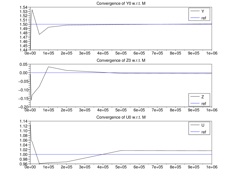
Figure 1: Evolution of $(Y^{q,p,N,M}_{0},Z^{q,p,N,M}_{0},U^{q,p,N,M}_{0})$ with respect to $M$ when $p=2$, $N=20$, $q=5$, $c=0.5$, $T=1$

Table 1 gives the computational time needed by the algorithm with this choice for $q$, $p$, $N$ and for different values of $M$. We notice from Figure 1 that the value of $(Y^{q,p,N,M}_{0},Z^{q,p,N,M}_{0},$ $U^{q,p,N,M}_{0})$ is close to the true solution from $M=2\times 10^{5}$. When $M=2\times 10^{5}$, the CPU time is about $1$ minute, which is quite small.

M	$10^{3}$	$5\times 10^{3}$	$10^{4}$	$5\times 10^{4}$	$10^{5}$	$2\times 10^{5}$	$5\times 10^{5}$	$10^{6}$
CPU time (in $s$)	0.253	1.277	2.567	13.24	26.81	56.91	142.75	283.65

Table 1: CPU time w.r.t. $M$ when $p=2$, $N=20$, $q=5$, $c=0.5$, $T=1$

5.2.2 Second example

We consider now the following BSDE

$$dY_{t}=-(\alpha Y_{t}+\beta Z_{t}+\gamma U_{t})dt+Z_{t}dB_{t}+U_{t}d\tilde{N}_{t},$$

$$\xi=\exp(aT+bB_{T}+cN_{T}).$$

The explicit solution is given by

$$Y_{t}=e^{aT+bB_{t}+cN_{t}}e^{(\alpha+\frac{(b+\beta)^{2}-\beta^{2}}{2})(T-t)+(e^{c}-1)(\kappa+\gamma)(T-t)},$$

$$Z_{t}=\mathbb{E}_{t^{-}}(D_{t}^{0}Y_{t})=bY_{t^{-}},\;\;U_{t}=\mathbb{E}_{t-}(D_{t}^{1}Y_{t})=(e^{c}-1)Y_{t-}$$

We choose $\alpha=\beta=0.3$, $\gamma=0.2$, $a=-0.1$, $b=0.1$, $c=0.2$, $\kappa=3$ and $T=2$. For these values, we get $(Y_{0},Z_{0},U_{0})=(6.599,0.66,1.4612)$. For $M=4\times 10^{5}$, $p=2$, $N=50$ and $q=10$, we get $(Y^{q,p,N,M}_{0},Z^{q,p,N,M}_{0},U^{q,p,N,M}_{0})=(6.560,0.56,1.294)$. We plot one path of $(Y^{q,p,N,M}_{t},Y_{t})_{t\leq T}$, $(Z^{q,p,N,M}_{t},Z_{t})_{t\leq T}$ and $(U^{q,p,N,M}_{t},U_{t})_{t\leq T}$ in Figures 2, 3, 4 with $M=4\times 10^{5}$, $p=2$, $N=50$ and $q=10$.

Figure 2: One path of $(Y^{q,p,N,M},Y)$

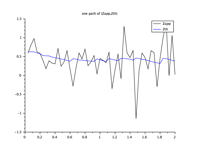
Figure 3: One path of $(Z^{q,p,N,M},Z)$

Figure 4: One path of $(U^{q,p,N,M},U)$

Appendix A Technical results

A.1 Proof of Lemmas 4.25 and 4.26

A.1.1 Proof of Lemma 4.25

Let $\tilde{t}_{l}:=\max\{t_{1},\cdots,t_{l}\}$. First, we prove by induction that $\forall q^{\prime}\leq q$, $(Y^{q^{\prime}},Z^{q^{\prime}},U^{q^{\prime}})$ belongs to $\mathcal{S}^{m,\infty}$, i.e. $\forall j\geq 2$

$$\|(Y^{q^{\prime}},Z^{q^{\prime}},U^{q^{\prime}})\|^{j}_{m,j}=\sum_{1\leq l\leq m}\sum_{\mathbf{i}_{l}}\operatorname*{ess\,sup}_{t_{1},\cdots,t_{l}} \left\{\mathbb{E}[\sup_{\tilde{t}_{l}\leq r\leq T}|D^{\mathbf{i}_{l}}_{t_{1},\cdots,t_{l}}Y^{q^{\prime}}_{r}|^{j}]+\int_{\tilde{t}_{l}}^{T}\mathbb{E}[|D^{\mathbf{i}_{l}}_{t_{1},\cdots,t_{l}}Z^{q^{\prime}}_{r}|^{j}]dr\right.$$

$$\left.+\int_{\tilde{t}_{l}}^{T}\mathbb{E}[|D^{\mathbf{i}_{l}}_{t_{1},\cdots,t_{l}}U^{q^{\prime}}_{r}|^{j}]dr\right\}<\infty.$$

Let $r\geq\tilde{t}_{l}$. Using (29) gives

$$D^{\mathbf{i}_{l}}_{t_{1},\cdots,t_{l}}Y^{q^{\prime}}_{r}=\mathbb{E}_{r}[D^{\mathbf{i}_{l}}_{t_{1},\cdots,t_{l}}F^{q^{\prime}-1}]-\!\int_{\tilde{t}_{l}}^{r}\!D^{\mathbf{i}_{l}}_{t_{1},\cdots,t_{l}}f(\theta^{q^{\prime}-1}_{s})ds,\,\mbox{where $\theta^{q^{\prime}-1}_{s}:=(s,Y^{q^{\prime}-1}_{s},Z^{q^{\prime}-1}_{s},U^{q^{\prime}-1}_{s})$.}$$

Using the Definition of $F^{q^{\prime}-1}$ and applying Doob’s inequality leads to

$$\mathbb{E}[\sup_{t_{l}\leq r\leq T}|D^{\mathbf{i}_{l}}_{t_{1},\cdots,t_{l}}Y^{q^{\prime}}_{r}|^{j}]\leq C(j)\left(\mathbb{E}[|D^{\mathbf{i}_{l}}_{t_{1},\cdots,t_{l}}\xi|^{j}]+\mathbb{E}\left(\int_{\tilde{t}_{l}}^{T}|D^{\mathbf{i}_{l}}_{t_{1},\cdots,t_{l}}f(\theta^{q^{\prime}-1}_{s})|^{j}ds\right)\right),$$

where $C(j)$ is a generic constant depending also on $T$. Analyzing the outcome of the repeated Malliavin derivative where for $D^{(0)}_{t}f(\theta^{q^{\prime}-1}_{s})$ the chain rule holds while

$$D^{(1)}_{t}f(\theta^{q^{\prime}-1}_{s})=f(s,Y^{q^{\prime}-1}_{s}+D^{(1)}_{t}Y^{q^{\prime}-1}_{s},Z^{q^{\prime}-1}_{s}+D^{(1)}_{t}Z^{q^{\prime}-1}_{s},U^{q^{\prime}-1}_{s}+D^{(1)}_{t}U^{q^{\prime}-1}_{s})-f(\theta^{q^{\prime}-1}_{s})$$

(see, for example, [9, Lemma 3.2]), one can see that the term $|D^{\mathbf{i}_{l}}_{t_{1},\cdots,t_{l}}f(\theta^{q^{\prime}-1}_{s})|$ is bounded by a sum of terms of type

$$\left(\sum_{k=1}^{l_{0}+l_{1}+l_{2}}\|\partial_{sp}^{k}f\|_{\infty}\right)\left|D^{\mathbf{k}_{0}}_{\mathbf{t}_{0}}Y_{s}^{q^{\prime}-1}\right|\left|D^{\mathbf{k}_{1}}_{\mathbf{t}_{1}}Z_{s}^{q^{\prime}-1}\right|\left|D^{\mathbf{k}_{2}}_{\mathbf{t}_{2}}U_{s}^{q^{\prime}-1}\right|,$$

where $\mathbf{k}_{j}\in\{0,1\}^{l_{j}}$ are vectors of size $l_{j}$ and $l_{0}+l_{1}+l_{2}\leq l.$ Then, Hölder’s inequality gives

$$\mathbb{E}\left(\int_{\tilde{t}_{l}}^{T}|D^{\mathbf{i}_{l}}_{t_{1},\cdots,t_{l}}f(\theta^{q^{\prime}-1}_{s})|^{j}ds\right)\leq C\left(\sum_{k=1}^{l}\|\partial^{k}_{sp}f\|^{j}_{\infty}\right)\|(Y^{q^{\prime}-1},Z^{q^{\prime}-1},U^{q^{\prime}-1})\|^{lj}_{l,lj}$$ (48)

and

$$\sum_{1\leq l\leq m}\sum_{\mathbf{i}_{l}\in\{0,1\}^{l}} \operatorname*{ess\,sup}_{t_{1},\cdots,t_{l}}\,\mathbb{E}[\sup_{t_{l}\leq r\leq T}|D^{\mathbf{i}_{l}}_{t_{1},\cdots,t_{l}}Y^{q^{\prime}}_{r}|^{j}]$$

$$\leq C(j)\left(\|\xi\|^{j}_{m,j}+\sum_{l=1}^{m}\left(\sum_{k=1}^{l}\|\partial^{k}_{sp}f\|^{j}_{\infty}\right)\|(Y^{q^{\prime}-1},Z^{q^{\prime}-1},U^{q^{\prime}-1})\|^{lj}_{l,lj}\right).$$ (49)

From (30), we get $D^{\mathbf{i}_{l}}_{t_{1},\cdots,t_{l}}Z^{q^{\prime}}_{r}=\mathbb{E}_{r}[D^{(i_{1},\cdots,i_{l},0)}_{t_{1},\cdots,t_{l},r}\xi+\int_{r}^{T}D^{(i_{1},\cdots,i_{l},0)}_{t_{1},\cdots,t_{l},r}f(\theta^{q^{\prime}-1}_{u})du]\mathbf{1}_{\{r\geq\tilde{t}_{l}\}}$. Then

$$\int_{\tilde{t}_{l}}^{T}\mathbb{E}[|D^{\mathbf{i}_{l}}_{t_{1},\cdots,t_{l}} Z^{q^{\prime}}_{r}|^{j}]dr$$

$$\leq C(j)\left(\int_{\tilde{t}_{l}}^{T}\mathbb{E}[|D^{(i_{1},\cdots,i_{l},0)}_{t_{1},\cdots,t_{l},r}\xi|^{j}]dr+\int_{\tilde{t}_{l}}^{T}\mathbb{E}\left(\left|\int_{r}^{T}D^{(i_{1},\cdots,i_{l},0)}_{t_{1},\cdots,t_{l},r}f(\theta^{q^{\prime}-1}_{u})du\right|^{j}\right)dr\right).$$

Using (48) yields

$$\sum_{1\leq l\leq m}\sum_{\mathbf{i}_{l}\in\{0,1\}^{l}} \operatorname*{ess\,sup}_{t_{1},\cdots,t_{l}}\,\int_{\tilde{t}_{l}}^{T}\mathbb{E}[|D^{\mathbf{i}_{l}}_{t_{1},\cdots,t_{l}}Z^{q^{\prime}}_{r}|^{j}]dr$$

$$\leq C(j)\left(\|\xi\|^{j}_{m+1,j}+\sum_{l=1}^{m}\left(\sum_{k=1}^{l+1}\|\partial^{k}_{sp}f\|^{j}_{\infty}\right)\|(Y^{q^{\prime}-1},Z^{q^{\prime}-1},U^{q^{\prime}-1})\|^{(l+1)j}_{(l+1),(l+1)j}\right).$$

The same type of result holds for $\int_{\tilde{t}_{l}}^{T}\mathbb{E}[|D^{\mathbf{i}_{l}}_{t_{1},\cdots,t_{l}}U^{q^{\prime}}_{r}|^{j}]dr$. Combining this result with (A.1.1) gives

$$\|(Y^{q^{\prime}},Z^{q^{\prime}},U^{q^{\prime}})\|^{j}_{m,j}\leq C(j)\!\left(\!\|\xi\|^{j}_{m+1,j}+\left(\sum_{k=1}^{m+1}\|\partial^{k}_{sp}f\|^{j}_{\infty}\!\right)\sum_{l=1}^{m}\|(Y^{q^{\prime}-1},Z^{q^{\prime}-1},U^{q^{\prime}-1})\|^{(l+1)j}_{(l+1),(l+1)j}\right).$$

Iterating this inequality yields the result.

A.1.2 Proof of Lemma 4.26

We prove it by induction on $q.$ Let $r\geq\tilde{t}_{l}\!:=\max\{t_{1},\cdots,t_{l}\}$ and $\theta^{q,p}_{s}:=(s,Y^{q,p}_{s},Z^{q,p}_{s},U^{q,p}_{s}).$ From (31) we get that

$$D^{\mathbf{i}_{l}}_{t_{1},\cdots,t_{l}}Y^{q+1,p}_{r} =\mathbb{E}_{r}[D^{\mathbf{i}_{l}}_{t_{1},\cdots,t_{l}}\mathcal{C}_{p}(F^{q,p})]-\int_{\tilde{t}_{l}}^{r}D^{\mathbf{i}_{l}}_{t_{1},\cdots,t_{l}}f(\theta^{q,p}_{s})ds$$

$$=\mathbb{E}_{r}[\mathcal{C}_{p-l}(D^{\mathbf{i}_{l}}_{t_{1},\cdots,t_{l}}F^{q,p})]\mathbf{1}_{\{l\leq p\}}-\int_{\tilde{t}_{l}}^{r}D^{\mathbf{i}_{l}}_{t_{1},\cdots,t_{l}}f(\theta^{q,p}_{s})ds,$$

where we have used Lemma 2.13 to get the second equality. Applying Doob’s maximal inequality leads to

$$\mathbb{E}[\sup_{\tilde{t}_{l}\leq r\leq T}|D^{\mathbf{i}_{l}}_{t_{1},\cdots,t_{l}}Y^{q+1,p}_{r}|^{j}]\leq C(j)\bigg{(}\mathbb{E}[|\mathcal{C}_{p-l}(D^{\mathbf{i}_{l}}_{t_{1},\cdots,t_{l}}F^{q,p})|^{j}]\mathbf{1}_{\{l\leq p\}}$$

$$\quad\quad\quad+\mathbb{E}\left(\int_{\tilde{t}_{l}}^{T}|D^{\mathbf{i}_{l}}_{t_{1},\cdots,t_{l}}f(\theta^{q,p}_{s})|^{j}ds\right)\bigg{)},$$ (50)

where $C(j)$ is a generic constant depending also on $T$. Let us first deal with the first term of the r.h.s. of (A.1.2), we assume $l\leq p$. Following Proposition 2.7, we know that $F^{q,p}=\sum_{n=0}^{\infty}I_{n}(g_{n})$. Then

$$D^{\mathbf{i}_{l}}_{t_{1},\cdots,t_{l}}F^{q,p} =\sum_{n=l}^{\infty}n(n-1)\cdots(n-l+1)I_{n-l}(g_{n}(*,z_{1},\cdots,z_{l})),$$

with $z_{k}=(t_{k},i_{k})$ and

$$\mathcal{C}_{p-l}(D^{\mathbf{i}_{l}}_{t_{1},\cdots,t_{l}}F^{q,p}) =\sum_{n=l}^{p}n(n-1)\cdots(n-l+1)I_{n-l}(g_{n}(*,z_{1},\cdots,z_{l})),$$

$$=\sum_{n=0}^{p-l}\frac{(n+l)!}{n!}I_{n}(g_{n+l}(*,z_{1},\cdots,z_{l})).$$

Let us denote $\hat{g}_{n_{i}}(*):=g_{n_{i}+l}(*,z_{1},\cdots,z_{l})$. From Proposition 2.11 we get

$$\mathbb{E}[|\mathcal{C}_{p-l}(D^{\mathbf{i}_{l}}_{t_{1},\cdots,t_{l}}F^{q,p})|^{j}]$$

$$=\sum_{n_{1},\cdots,n_{j}=0}^{p-l}\mathbb{E}(I_{n_{1}}(\hat{g}_{n_{1}})\cdots I_{n_{j}}(\hat{g}_{n_{j}}))\frac{(n_{1}+l)!}{n_{1}!}\cdots\frac{(n_{j}+l)!}{n_{j}!}$$

$$=\sum_{n_{1},\cdots,n_{j}=0}^{p-l}\!\!\!\frac{(n_{1}+l)!}{n_{1}!}\cdots\frac{(n_{j}+l)!}{n_{j}!}\!\!\!\sum_{J^{B}\in[n]}\,\,\sum_{(\tau,\sigma)\in\Pi_{=2,\geq 2}(J^{B};n_{1},\ldots,n_{j})}\kappa^{|\sigma|}\int_{[0,T]^{|\tau|+|\sigma|}}\bigg{(}\bigotimes_{i=1}^{j}\hat{g}_{n_{i}}\bigg{)}_{\tau\cup\sigma}d\lambda^{|\tau|+|\sigma|}$$

$$\leq\sum_{n_{1},\cdots,n_{j}=0}^{p-l}\frac{(n_{1}+l)!}{n_{1}!}\cdots\frac{(n_{j}+l)!}{n_{j}!}\prod_{i=1}^{j}\|g_{n_{i}+l}\|_{\infty}\sum_{J^{B}\in[n]}\,\,\sum_{(\tau,\sigma)\in\Pi_{=2,\geq 2}(J^{B};n_{1},\ldots,n_{j})}\kappa^{|\sigma|}\,T^{|\tau|+|\sigma|}.$$ (51)

Thanks to the assumptions on $f$ and $\xi$ and induction hypothesis, we have $F^{q,p}\in\mathbb{D}^{p,2}$. Then, (14) gives that $g_{n_{i}+l}(z_{1},\cdots,z_{n_{i}+l})=\frac{1}{(n_{i}+l)!}\mathbb{E}(D^{(i_{1},\cdots,i_{n_{i}+l})}_{t_{1},\cdots,t_{n_{i}+l}}(F^{q,p}))$, then $\|g_{n_{i}+l}\|_{\infty}\leq\frac{1}{(n_{i}+l)!}\|F^{q,p}\|_{n_{i}+l,1}$. Since $n_{i}\leq p-l$, we get $\|g_{n_{i}+l}\|_{\infty}\leq\frac{1}{(n_{i}+l)!}\|F^{q,p}\|_{p,1}$. Then

$$\mathbb{E}[|\mathcal{C}_{p-l}(D^{\mathbf{i}_{l}}_{t_{1},\cdots,t_{l}}F^{q,p})|^{j}] \leq(\|F^{q,p}\|_{p,1})^{j}\sum_{n_{1},\cdots,n_{j}=0}^{p-l}\sum_{J^{B}\in[n]}\,\,\sum_{(\tau,\sigma)\in\Pi_{=2,\geq 2}(J^{B};n_{1},\ldots,n_{j})}\kappa^{|\sigma|}\,T^{|\tau|+|\sigma|}$$

$$\leq C(p,j)(\|F^{q,p}\|_{p,1})^{j}.$$ (52)

We have $\|F^{q,p}\|_{p,1}=\sum_{l\leq p}\sum_{\mathbf{i}_{l}\in\{0,1\}^{l}}\operatorname*{ess\,sup}_{t_{1},\cdots,t_{l}}\mathbb{E}(|D_{t_{1},\cdots,t_{l}}^{\mathbf{i}_{l}}F^{q,p}|)$ where

$$\mathbb{E}(|D_{t_{1},\cdots,t_{l}}^{\mathbf{i}_{l}}F^{q,p}|)\leq\mathbb{E}(|D_{t_{1},\cdots,t_{l}}^{\mathbf{i}_{l}}\xi|)+\mathbb{E}(\int_{\tilde{t}_{l}}^{T}|D_{t_{1},\cdots,t_{l}}^{\mathbf{i}_{l}}f(\theta_{s}^{q,p})|ds).$$

By using (48), we get $\mathbb{E}\left(\int_{\tilde{t}_{l}}^{T}|D^{\mathbf{i}_{l}}_{t_{1},\cdots,t_{l}}f(\theta^{q,p}_{s})|ds\right)\leq C\left(\sum_{k=1}^{l}\|\partial^{k}_{sp}f\|_{\infty}\right)\|(Y^{q,p},Z^{q,p},U^{q,p})\|^{l}_{l,l}$. Then

$$\|F^{q,p}\|_{p,1} \leq\|\xi\|_{p,1}+\sum_{l\leq p}C\left(\sum_{k=1}^{l}\|\partial^{k}_{sp}f\|_{\infty}\right)\|(Y^{q,p},Z^{q,p},U^{q,p})\|^{l}_{l,l},$$ (53)

$$\|F^{q,p}\|_{p,1}^{j} \leq C(p,j)\left(\|\xi\|^{j}_{p,1}+\sum_{l\leq p}C\left(\sum_{k=1}^{l}\|\partial^{k}_{sp}f\|^{j}_{\infty}\right)\|(Y^{q,p},Z^{q,p},U^{q,p})\|^{lj}_{l,lj}\right).$$ (54)

Let us now deal with the second term of the r.h.s. of (A.1.2). By using (48), we get

$$\mathbb{E}\left(\int_{\tilde{t}_{l}}^{T}|D^{\mathbf{i}_{l}}_{t_{1},\cdots,t_{l}}f(\theta^{q,p}_{s})|^{j}ds\right)\leq C\left(\sum_{k=1}^{l}\|\partial^{k}_{sp}f\|^{j}_{\infty}\right)\|(Y^{q,p},Z^{q,p},U^{q,p})\|^{lj}_{l,lj}.$$ (55)

Combining (A.1.2), (54), (55) and (A.1.2) yields

$$\mathbb{E}[\sup_{\tilde{t}_{l}\leq r\leq T}|D^{\mathbf{i}_{l}}_{t_{1},\cdots,t_{l}}Y^{q+1,p}_{r}|^{j}]$$

$$\leq C(p,j)\left(\|\xi\|^{j}_{p,1}+\sum_{l\leq p}C\left(\sum_{k=1}^{l}\|\partial^{k}_{sp}f\|^{j}_{\infty}\right)\|(Y^{q,p},Z^{q,p},U^{q,p})\|^{lj}_{l,lj}\right)\mathbf{1}_{\{l\leq p\}}$$

$$+C\left(\sum_{k=1}^{l}\|\partial^{k}_{sp}f\|^{j}_{\infty}\right)\|(Y^{q,p},Z^{q,p},U^{q,p})\|^{lj}_{l,lj},$$

and

$$\sum_{1\leq l\leq m}\sum_{\mathbf{i}_{l}\in\{0,1\}^{l}}\operatorname*{ess\,sup}_{t_{1},\cdots,t_{l}}\mathbb{E}[\sup_{\tilde{t}_{l}\leq r\leq T}|D^{\mathbf{i}_{l}}_{t_{1},\cdots,t_{l}}Y^{q+1,p}_{r}|^{j}]$$

$$\leq C(p,j)\left(\|\xi\|^{j}_{p,1}+\sum_{l=1}^{m\vee p}C\left(\sum_{k=1}^{l}\|\partial^{k}_{sp}f\|^{j}_{\infty}\right)\|(Y^{q,p},Z^{q,p},U^{q,p})\|^{lj}_{l,lj}\right).$$ (56)

From (32) we get

$$D^{(i_{1},\cdots,i_{l})}_{t_{1},\cdots,t_{l}}Z^{q+1,p}_{r}=\mathbb{E}_{r}[D^{(i_{1},\cdots,i_{l},0)}_{t_{1},\cdots,t_{l},r}\mathcal{C}_{p}(F^{q,p})]=\mathbb{E}_{r}[\mathcal{C}_{p-l-1}(D^{(i_{1},\cdots,i_{l},0)}_{t_{1},\cdots,t_{l},r}F^{q,p})]\mathbf{1}_{\{l\leq p-1\}}\mathbf{1}_{\{r\geq\tilde{t}_{l}\}}.$$

Then

$$\int_{\tilde{t}_{l}}^{T}\mathbb{E}[|D^{\mathbf{i}_{l}}_{t_{1},\cdots,t_{l}}Z^{q+1,p}_{r}|^{j}]dr\leq C\left(\int_{\tilde{t}_{l}}^{T}\mathbb{E}[|\mathcal{C}_{p-l-1}(D^{(i_{1},\cdots,i_{l},0)}_{t_{1},\cdots,t_{l},r}F^{q,p})|^{j}]dr\right)\mathbf{1}_{\{l\leq p-1\}}.$$

Using (A.1.2) and (54) leads to

$$\sum_{1\leq l\leq m}\sum_{\mathbf{i}_{l}\in\{0,1\}^{l}}\operatorname*{ess\,sup}_{t_{1},\cdots,t_{l}}\int_{\tilde{t}_{l}}^{T}\mathbb{E}[|D^{\mathbf{i}_{l}}_{t_{1},\cdots,t_{l}}Z^{q+1,p}_{r}|^{j}]dr$$

$$\leq C(p,j)\left(\|\xi\|^{j}_{p,1}+\sum_{l=1}^{p}C\left(\sum_{k=1}^{l}\|\partial^{k}_{sp}f\|^{j}_{\infty}\right)\|(Y^{q,p},Z^{q,p},U^{q,p})\|^{lj}_{l,lj}\right).$$

The same type of result holds for $\int_{\tilde{t}_{l}}^{T}\mathbb{E}[|D^{\mathbf{i}_{l}}_{t_{1},\cdots,t_{l}}U^{q+1,p}_{r}|^{j}]dr$. Combining these results with (A.1.2) gives

$$\|(Y^{q+1,p},Z^{q+1,p},U^{q+1,p})\|^{j}_{m,j}\leq\!C(p,j)\left(\|\xi\|^{j}_{p,1}+\sum_{l=1}^{m\vee p}C\left(\sum_{k=1}^{l}\|\partial^{k}_{sp}f\|^{j}_{\infty}\right)\|(Y^{q,p},Z^{q,p},U^{q,p})\|^{lj}_{l,lj}\right).$$

Iterating this inequality yields the result.

A.2 Proof of Lemma 4.29

We will prove the assertion by induction in $p\in\mathbb{N}.$ Since $(\mathcal{C}_{0}^{N})(F)=(\mathcal{C}_{0})(F)$ Lemma 4.29 holds for $p=0.$ Assume that for $p\in\mathbb{N}^{*}$

$$\mathbb{E}|(\mathcal{C}_{p-1}^{N}-\mathcal{C}_{p-1})(F)|^{2}\leq\sum_{j=1}^{p-1}(K_{j}^{F})^{2}\bigg{(}\frac{T}{N}\bigg{)}^{2\beta_{F}}\sum_{i=1}^{p-1}i^{2}\frac{T^{i}}{i!}.$$

By using (5) and (2.3), we get

$$(\mathcal{C}_{p}^{N}-\mathcal{C}_{p})(F)=(\mathcal{C}_{p-1}^{N}-\mathcal{C}_{p-1})(F)+(P_{p}^{N}-P_{p})(F).$$

Then, it suffices to show that

$$\mathbb{E}|(P_{p}^{N}-P_{p})(F)|^{2}\leq(K_{p}^{F})^{2}\left(\frac{T}{N}\right)^{2\beta_{F}}p^{2}\frac{T^{p}}{p!}.$$

We have $P_{p}(F)=I_{p}(g_{p})$ where we will assume that $g_{p}$ is symmetric. It holds

$$P^{N}_{p}(F)=I_{p}(g_{p}^{N})$$

with

$$g_{p}^{N}((t_{1},i_{1}),\cdots,(t_{p},i_{p}))= \sum_{{\bf k}_{p}\in\{1,\cdots,N\}^{p}}\langle g_{p}((\cdot,i_{1}),\cdots,(\cdot,i_{p})),e[k_{1},...,k_{p}]\rangle_{L^{2}([0,T]^{p})}$$

$$\quad\quad\quad\quad\times e[k_{1},...,k_{p}](t_{1},\cdots,t_{p}).$$

Then $g_{p}^{N}$ is constant w.r.t. $(t_{1},\cdots,t_{p})\in\Lambda_{{\bf k}_{p}}:=\Lambda_{k_{1}}\times\cdots\times\Lambda_{k_{p}}$ with $\Lambda_{i}:=]\overline{t}_{i-1},\overline{t}_{i}]$ since $e[k_{1},...,k_{p}]=h^{-\frac{p}{2}}\mathbf{1}_{\Lambda_{{\bf k}_{p}}}.$ We have by (13), (14) and (39) that

$$\mathbb{E}|(P_{p}^{N}-P_{p})(F)|^{2}$$

$$=\mathbb{E}|I_{p}(g_{p}^{N})-I_{p}(g_{p})|^{2}$$

$$=\sum_{{\bf k}_{p}}\sum_{{\bf i}_{p}}\kappa^{|{\bf i}_{p}|}p!\|h^{-\frac{p}{2}}\langle g_{p}((\cdot,i_{1}),\cdots,(\cdot,i_{p})),e[k_{1},...,k_{p}]\rangle_{L^{2}([0,T]^{p})}-g_{p}((\cdot,i_{1}),\cdots,(\cdot,i_{p}))\|^{2}_{L_{2}(\Lambda_{{\bf k}_{p}})}$$

$$=\sum_{{\bf k}_{p}}\sum_{{\bf i}_{p}}\kappa^{|{\bf i}_{p}|}p!\left\|h^{-p}\!\!\!\int_{\Lambda_{{\bf k}_{p}}}g_{p}((s_{1},i_{1}),\cdots,(s_{p},i_{p}))-g_{p}((\cdot,i_{1}),\cdots,(\cdot,i_{p}))ds_{1}...ds_{p}\right\|^{2}_{L_{2}(\Lambda_{{\bf k}_{p}})}$$

$$\leq\sum_{{\bf k}_{p}{\bf i}_{p}}\kappa^{|{\bf i}_{p}|}p!h^{-2p}\!\!\!\int_{\Lambda_{\mathbf{k}_{p}}}\!\!\!\left(\int_{\Lambda_{{\bf k}_{p}}}\!\!\!|g_{p}((s_{1},i_{1}),\cdots,(s_{p},i_{p}))-g_{p}((t_{1},i_{1}),\cdots,(t_{p},i_{p}))|ds_{1}...ds_{p}\!\right)^{2}\!\!\!dt_{1}\cdots dt_{p}$$

$$\leq\sum_{{\bf k}_{p}}\sum_{{\bf i}_{p}}\kappa^{|{\bf i}_{p}|}\frac{1}{p!}h^{-2p}\int_{\Lambda_{\mathbf{k}_{p}}}\left(\int_{\Lambda_{{\bf k}_{p}}}K^{F}_{p}(|t_{1}-s_{1}|^{\beta_{F}}+\cdots+|t_{p}-s_{p}|^{\beta_{F}})ds_{1}...ds_{p}\right)^{2}dt_{1}\cdots dt_{p}$$

$$\leq(K^{F}_{p})^{2}T^{p}(1+\kappa)^{p}p^{2}\frac{1}{p!}\big{(}\frac{T}{N}\big{)}^{2\beta_{F}}.$$

A.3 Proof of Lemma 4.30

We will show that if

$$(Y_{t}^{q,p},Z_{t}^{q,p},U_{t}^{q,p})\text{ satisfies }\mathcal{H}_{p}\text{ for a.e. }t\in[0,T]$$ (57)

(with $\beta_{I_{q,p}}=\frac{1}{2}\wedge\beta_{\xi}$) then also $I_{q,p}=\int_{0}^{T}f(s,Y_{s}^{q,p},Z_{s}^{q,p},U_{s}^{q,p})ds$ does satisfy $\mathcal{H}_{p}$. As $I_{0,p}$ is constant, it satisfies $\mathcal{H}_{p}$. For $q\geq 1$ we will use the notation $D_{\mathbf{t}}^{\alpha(1:i-1)}\Delta^{\alpha_{i}}_{i}D_{\mathbf{s}}^{\alpha(i+1:r)}F:=D^{(\alpha_{1},\cdots,\alpha_{i-1})}_{t_{1},\cdots,t_{i-1}}(D_{t_{i},s_{i+1},\cdots,s_{r}}^{(\alpha_{i},\cdots,\alpha_{r})}F-D_{s_{i},s_{i+1},\cdots,s_{r}}^{(\alpha_{i},\cdots,\alpha_{r})}F)$ and prove that for $1\leq r\leq p$

$$\mathbb{E}|D^{\alpha(1:i-1)}_{\mathbf{t}}\Delta^{\alpha_{i}}_{i}D^{\alpha(i+1:r)}_{\mathbf{s}}I_{q,p}|^{j}\leq K_{r}(j)|t_{i}-s_{i}|^{j\beta_{I_{q,p}}}$$

(that $\mathcal{H}^{1}_{p}$ holds for $I_{q,p}$ is clear). Setting $\mathbf{ts}_{-i}:=\max\{t_{1},\cdots,t_{i-1},s_{i+1},\cdots,s_{r}\}$ and $\theta_{u}^{q,p}:=(u,Y_{u}^{q,p},Z_{u}^{q,p},$ $U_{u}^{q,p})$ we have

$$D^{\alpha(1:i-1)}_{\mathbf{t}}\Delta^{\alpha_{i}}_{i}D^{\alpha(i+1:r)}_{\mathbf{s}}I_{q,p} =\int_{t_{i}\vee s_{i}\vee\mathbf{ts}_{-i}}^{T}D^{\alpha(1:i-1)}_{\mathbf{t}}\Delta^{\alpha_{i}}_{i}D^{\alpha(i+1:r)}_{\mathbf{s}}f(\theta_{u}^{q,p})du$$

$$\pm\int_{(t_{i}\wedge s_{i})\vee\mathbf{ts}_{-i}}^{t_{i}\vee s_{i}\vee\mathbf{ts}_{-i}}D^{\alpha(1:i-1)}_{\mathbf{t}}D^{\alpha_{i}}_{t_{i}\wedge s_{i}}D^{\alpha(i+1:r)}_{\mathbf{s}}f(\theta_{u}^{q,p})du,$$ (58)

where $\pm=-$ for $t_{i}>s_{i},$ and $\pm=+$ for the opposite case. From the proof of Lemma 4.25 we know that $|D^{\alpha(1:i-1)}_{\mathbf{t}}D^{\alpha_{i}}_{t_{i}\wedge s_{i}}D^{\alpha(i+1:r)}_{\mathbf{s}}f(\theta_{u}^{q,p})|$ is bounded by a sum of terms of type

$$\left(\sum_{j=1}^{r}\|\partial_{sp}^{j}f\|_{\infty}\right)|D^{\mathbf{k}_{0}}_{\mathbf{t}_{0}}Y_{u}^{q,p}|\,|D^{\mathbf{k}_{1}}_{\mathbf{t}_{1}}Z_{u}^{q,p}|\,|D^{\mathbf{k}_{2}}_{\mathbf{t}_{2}}U_{u}^{q,p}|,$$

where $\mathbf{k}_{j}\in\{0,1\}^{l_{j}}$ are vectors of size $l_{j}$ with $l_{0}+l_{1}+l_{2}\leq r$ and $\mathbf{t}_{j}$ are sub vectors of $\{t_{1},...,t_{i-1},t_{i}\wedge s_{i},s_{i+1},...,s_{r}\}.$ Hölder’s inequality and Lemma 4.26 give

$$\mathbb{E}\left|\int_{(t_{i}\wedge s_{i})\vee\mathbf{ts}_{-i}}^{t_{i}\vee s_{i}\vee\mathbf{ts}_{-i}}D^{\alpha(1:i-1)}_{\mathbf{t}}D^{\alpha_{i}}_{t_{i}\wedge s_{i}}D^{\alpha(i+1:r)}_{\mathbf{s}}f(\theta_{u}^{q,p})du\right|^{j}\leq C(p,j,\|\xi\|_{p,1},(\|\partial_{sp}^{k}f\|_{\infty})_{k\leq p})|t_{i}-s_{i}|^{\frac{j}{2}}.$$

For the first term on the r.h.s. of (A.3) we notice that

$$\int_{t_{i}\vee s_{i}\vee\mathbf{ts}_{-i}}^{T}|D^{\alpha(1:i-1)}_{\mathbf{t}}\Delta^{\alpha_{i}}_{i}D^{\alpha(i+1:r)}_{\mathbf{s}}f(\theta_{u}^{q,p})|du$$

is bounded by a sum of terms of type

$$\int_{\mathbf{ts}_{-i}}^{T}\bigg{(}\sum_{j=1}^{r}\|\partial_{sp}^{j}f\|_{\infty}\bigg{)}|D^{\mathbf{k}_{0}}_{\mathbf{t}_{0}}\Phi_{u}^{q,p}|\,|D^{\mathbf{k}_{1}}_{\mathbf{t}_{1}}\Psi_{u}^{q,p}|\,|D^{\mathbf{k}_{2}}_{\mathbf{t}_{2}}\Delta^{\alpha_{i}}_{i}D^{\mathbf{k}_{3}}_{\mathbf{t}_{3}}\Gamma_{u}^{q,p}|du,$$

where $(\Phi_{u}^{q,p},\Psi_{u}^{q,p},\Gamma_{u}^{q,p})$ stands for a permutation of $\{Y_{u}^{q,p},Z_{u}^{q,p},U_{u}^{q,p}\},$ and $\mathbf{k}_{j}\in\{0,1\}^{l_{j}}$ are vectors of size $l_{0},l_{1},l_{2}+l_{3}+1\leq r$ while the $\mathbf{t}_{j}$ denote the appropriate sub vectors of $\{t_{1},...,t_{i-1},t_{i},s_{i},s_{i+1},...,s_{r}\}.$

By Hölder’s inequality and assumption (57) we conclude that

$$\mathbb{E}\left|\int_{t_{i}\vee s_{i}\vee\mathbf{ts}_{-i}}^{T}D^{\alpha(1:i-1)}_{\mathbf{t}}\Delta^{\alpha_{i}}_{i}D^{\alpha(i+1:r)}_{\mathbf{s}}f(\theta_{u}^{q,p})du\right|^{j}\leq K_{r}(j)|t_{i}-s_{i}|^{j\beta_{I_{q,p}}}.$$

We finish the proof of Lemma 4.30 by arguing that assumption (57) holding for true for a certain $q,$ implies it for $q+1:$ We want to use (31) and (32) and therefore we first notice that in the same way as above for $I_{q,p}$ one can show that (57) implies that

$$\int_{0}^{t}f\left(s,Y^{q,p}_{s},Z^{q,p}_{s},U^{q,p}_{s}\right)ds\text{ \,\,\, satisfies \,\,\,}\mathcal{H}_{p}.$$

It is also clear that satisfying $\mathcal{H}_{p}$ is stable with respect to linear combination and taking the conditional expectation $\mathbb{E}_{t}.$ What we still need to check is whether satisfying $\mathcal{H}_{p}$ is also stable with respect to the truncation $\mathcal{C}_{p}.$ For this, let us assume that $F=\sum_{n=0}^{\infty}I_{n}(g_{n})$ satisfies $\mathcal{H}_{p}.$ Following the proof of Lemma 4.26, we have

$$D^{\alpha(1:i-1)}_{\mathbf{t}}\Delta^{\alpha_{i}}_{i}D^{\alpha(i+1:r)}_{\mathbf{s}}F$$

$$=\sum_{n=r}^{\infty}n(n-1)\cdots(n-r+1)I_{n-r}(g_{n}(*,z_{1},\cdots,z_{i},z^{\prime}_{i+1},\cdots,z^{\prime}_{r})$$

$$\quad\quad\quad\quad\quad\quad-g_{n}(*,z_{1},\cdots,z_{i-1},z^{\prime}_{i}\cdots,z^{\prime}_{r})),$$

where $z_{j}=(t_{j},i_{j})$ and $z^{\prime}_{j}=(s_{j},i_{j}).$ Like in (A.1.2) we get

$$\mathbb{E}[|\mathcal{C}_{p-r}(D^{\alpha(1:i-1)}_{\mathbf{t}}\Delta^{\alpha_{i}}_{i}D^{\alpha(i+1:r)}_{\mathbf{s}}F)|^{j}]$$

$$\leq C(p,j,T)\sum_{n_{1},\cdots,n_{j}=0}^{p-r}\frac{(n_{1}+r)!}{n_{1}!}\cdots\frac{(n_{j}+r)!}{n_{j}!}$$

$$\,\,\times\prod_{i=1}^{j}\|g_{n_{i}+r}(*,z_{1},\cdots,z_{i},z^{\prime}_{i+1},\cdots,z^{\prime}_{r})-g_{n_{i}+r}(*,z_{1},\cdots,z_{i-1},z^{\prime}_{i}\cdots,z^{\prime}_{r}))\|_{\infty}$$

$$\leq C(p,j,T)(K_{p}^{F}(1)|t_{i}-s_{i}|^{\beta_{F}})^{j},$$

where we used that

$$(n_{i}+r)!\|g_{n_{i}+r}(*,z_{1},\cdots,z_{i},z^{\prime}_{i+1},\cdots,z^{\prime}_{r})- g_{n_{i}+r}(*,z_{1},\cdots,z_{i-1},z^{\prime}_{i}\cdots,z^{\prime}_{r}))\|_{\infty}$$

$$\leq K_{p}^{F}(1)|t_{i}-s_{i}|^{\beta_{F}}.$$

A.4 Proof of Lemma 4.32

Using the definitions (27) and (36) leads to

$$(\mathcal{C}_{p}^{N}-\mathcal{C}_{p}^{N,M})(F)=d_{0}-\hat{d_{0}}+\sum_{k=1}^{p}\sum_{|{\bf n}|=k}(d^{\bf n}_{k}-\hat{d^{\bf n}_{k}})\prod_{i=1}^{N}K_{n_{i}^{B}}(G_{i})C_{n_{i}^{P}}(Q_{i},\kappa h).$$

Since $\hat{d^{\bf n}_{k}}$ is independent of $(G_{i},Q_{i})_{1\leq i\leq N}$

$$\mathbb{E}(|(\mathcal{C}_{p}^{N}-\mathcal{C}_{p}^{N,M})(F)|^{2})=\mathbb{E}(|d_{0}-\hat{d_{0}}|^{2})+\sum_{k=1}^{p}\sum_{|{\bf n}|=k}\frac{({\bf n}^{P})!(\kappa h)^{|{\bf n}^{P}|}}{({\bf n}^{B})!}\mathbb{E}(|d^{\bf n}_{k}-\hat{d^{\bf n}_{k}}|^{2}).$$

The definition of the coefficients $d_{0}$ and $d^{\bf n}_{k}$ given in (28) leads to

$$\mathbb{E}(|(\mathcal{C}_{p}^{N}-\mathcal{C}_{p}^{N,M})(F)|^{2})=\mathbb{V}(\hat{d_{0}})+\sum_{k=1}^{p}\sum_{|{\bf n}|=k}\frac{({\bf n}^{P})!(\kappa h)^{|{\bf n}^{P}|}}{({\bf n}^{B})!}\mathbb{V}(\hat{d^{\bf n}_{k}}).$$

Using the definition of $\hat{d^{\bf n}_{k}}$ (see (35)) leads to the first result. To get the second result, we write $\mathcal{C}_{p}^{N,M}(F)=(\mathcal{C}_{p}^{N,M}-\mathcal{C}_{p}^{N})(F)+\mathcal{C}_{p}^{N}(F)$. Since $\mathbb{E}\left((\mathcal{C}_{p}^{N,M}-\mathcal{C}_{p}^{N})(F)\mathcal{C}_{p}^{N}(F)\right)=0$, we get

$$\mathbb{E}(|\mathcal{C}_{p}^{N,M}(F)|^{2})=\mathbb{E}(|(\mathcal{C}_{p}^{N,M}-\mathcal{C}_{p}^{N})(F)|^{2})+\mathbb{E}(|\mathcal{C}_{p}^{N}(F)|^{2}).$$

Lemma 2.16 ends the proof.

A.5 The product of two multiple integrals

For the convenience of the reader, we cite here [14, Theorem 3.6] from Lee and Shih adapted to our simple situation where the multiple integrals $I_{k}(g_{k})$ are built using the process $B+\tilde{N}$ like in Subsection 2.1.2. For this, we first introduce the ’contraction and identification operator’ $\otimes_{a}^{b}.$ For symmetric functions $g_{k}\in(L^{2})^{\otimes k}(\lambda\otimes(\delta_{0}+\kappa\delta_{1}))$ and $g_{m}\in(L^{2})^{\otimes m}(\lambda\otimes(\delta_{0}+\kappa\delta_{1}))$ we define the function $g_{k}\otimes_{a}^{b}g_{m}:([0,T]\times\{0,1\})^{k-a-b}\times([0,T]\times\{0,1\})^{m-a-b}\times([0,T]\times\{0,1\})^{b}\to\mathbb{R}$ by

$$(g_{k}\otimes_{a}^{b}g_{m})({\bf x},{\bf y},{\bf z})=\int_{([0,T]\times\{0,1\})^{a}}g_{k}({\bf x},{\bf z},{\bf w})g_{m}({\bf w},{\bf z},{\bf y})d[\lambda\otimes(\delta_{0}+\kappa\delta_{1})]^{\otimes a}({\bf w})$$ (59)

for $({\bf x},{\bf y},{\bf z})\in([0,T]\times\{0,1\})^{k-a-b}\times([0,T]\times\{0,1\})^{m-a-b}\times([0,T]\times\{0,1\})^{b}.$

Theorem A.36.

If $g_{k}\in(L^{2})^{\otimes k}(\lambda\otimes(\delta_{0}+\kappa\delta_{1}))$ and $g_{m}\in(L^{2})^{\otimes m}(\lambda\otimes(\delta_{0}+\kappa\delta_{1}))$ are symmetric functions such that $|g_{k}|\otimes_{a}^{b}|g_{m}|$ is in $(L^{2})^{\otimes(k+m-2a-b)}(\lambda\otimes(\delta_{0}+\kappa\delta_{1})),$ then

$$I_{k}(g_{k})I_{m}(g_{m})=\sum_{a=0}^{k\wedge m}\sum_{b=0}^{k\wedge m-a}a!b!\binom{k}{a}\binom{m}{a}\binom{k-a}{b}\binom{m-a}{b}I_{k+m-2a-b}(g_{k}\otimes_{a}^{b}g_{m}).$$

An immediate consequence is that if $g_{k}$ and $g_{m}$ have disjoint support, then $I_{k}(g_{k})I_{m}(g_{m})=I_{k+m}(g_{k}\otimes g_{m}).$

References

References

- [1] D. Applebaum. Lévy Processes and Stochastic Calculus. Cambridge, 2009.
- [2] V. Bally and G. Pagès. A quantization algorithm for solving multi-dimensional discrete-time optimal stopping problems. Bernoulli, 9(6):1003–1049, 2003.
- [3] B. Bouchard and R. Elie. Discrete-time approximation of decoupled Forward-Backward SDE with jumps. Stochastic Processes and their Applications, 118:53–75, 2008.
- [4] B. Bouchard and N. Touzi. Discrete-time approximation and Monte-Carlo simulation of backward stochastic differential equations. Stochastic Process. Appl., 111(2):175–206, 2004.
- [5] P. Briand, B. Delyon, and J. Mémin. Donsker–type theorem for BSDEs. Electron. Comm. Probab., 6:1–14, 2001. (electronic).
- [6] P. Briand, B. Delyon, and J. Mémin. On the robustness of backward stochastic differential equations. Stochastic Process. Appl., 97(2):229–253, 2002.
- [7] P. Briand and C. Labart. Simulation of BSDEs by Wiener Chaos Expansion. Annals of Appl. Prob., 24(3):1129–1171, 2014.
- [8] C. Geiss and E. Laukkarinen. Density of certain smooth Lévy functionals in . Probab. Math. Statist., 31(1):1–15, 2011.
- [9] C. Geiss and A. Steinicke. L2-variation of Lévy driven BSDEs with non-smooth terminal conditions. Bernoulli, arXiv: 1404.4477, 2014.
- [10] E. Gobet, J.-P. Lemor, and X. Warin. A regression-based Monte Carlo method to solve backward stochastic differential equations. Ann. Appl. Probab., 15(3):2172–2202, 2005.
- [11] K. Itô. Spectral type of the shift transformation of differential process with stationary increments. Transactions of the American Mathematical Society, 81:253–263, 1956.
- [12] S. J.L., F. Utzet, and J. Vives. Chaos expansions and malliavin calculus for lévy processes. Stochastic analysis and applications, Abel Symp. 2:595–612, 2007.
- [13] G. Last, M. Penrose, M. Schulte, and C. Thäle. Moments and central limit theorems for some multivariate poisson functionals. arXiv: 1205.3033v3, 2014.
- [14] Y.-J. Lee and H.-H. Shih. The Product Formula of Multiple Lévy-Itô Integrals. Bulletin of the Institute of Mathematics Academia Sinica, 32(2), 2004.
- [15] A. Lejay, E. Mordecki, and S. Torres. Numerical approximation of Backward Stochastic Differential Equations with Jumps. http://hal.archives-ouvertes.fr/inria-00357992, 2014.
- [16] J. León, S. J.L., F. Utzet, and J. Vives. On Lévy processes, Malliavin calculus and market models with jumps. Finance and Stochastics, 6:197–225, 2002.
- [17] D. Nualart. The Malliavin calculus and related topics. Probability and its Applications (New York). Springer-Verlag, Berlin, second edition, 2006.
- [18] É. Pardoux and S. Peng. Backward stochastic differential equations and quasilinear parabolic partial differential equations. In B. L. Rozovskii and R. B. Sowers, editors, Stochastic partial differential equations and their applications (Charlotte, NC, 1991), volume 176 of Lecture Notes in Control and Inform. Sci., pages 200–217. Springer, Berlin, 1992.
- [19] G. Peccati and M. Taqqu. Wiener Chaos: Moments, Cumulants and Diagrams. Springer-Verlag, 2011.
- [20] E. Petrou. Malliavin calculus in Lévy spaces and applications to finance. Electron. J. Probab., 13:852–879, 2008.
- [21] N. Privault. Stochastic Analysis in Discrete and Continuous settings. With normal martingales. Lecture notes in Mathematics. Springer-Verlag, Berlin, 2009.
- [22] M. Schulte. Malliavin-Stein method in stochastic geometry. Osnabrück, 2013.
- [23] S. Tang and X. Li. Necessary conditions for optimal control of stochastic systems with random jumps. SIAM Journal on Control Optimization, 32(5):1447–1475, 1994.
- [24] J. Zhang. A numerical scheme for BSDEs. Ann. Appl. Probab., 14(1):459–488, 2004.