Holographic p-wave superconductor models with Weyl corrections

Abstract

Abstract

We study the effect of the Weyl corrections on the holographic p-wave dual models in the backgrounds of AdS soliton and AdS black hole via a Maxwell complex vector field model by using the numerical and analytical methods. We find that, in the soliton background, the Weyl corrections do not influence the properties of the holographic p-wave insulator/superconductor phase transition, which is different from that of the Yang-Mills theory. However, in the black hole background, we observe that similar to the Weyl correction effects in the Yang-Mills theory, the higher Weyl corrections make it easier for the p-wave metal/superconductor phase transition to be triggered, which shows that these two p-wave models with Weyl corrections share some similar features for the condensation of the vector operator.

I Introduction

As a brilliant concept, the anti-de Sitter/conformal field theory (AdS/CFT) correspondence conjectures a duality between strongly coupled quantum field theories and weakly coupled gravity theories Maldacena , which has become a powerful tool to study the condensed matter systems. It was shown that a gravitational model of hairy black holes GubserPRD78 , where the Abelian symmetry of Higgs is spontaneously broken below some critical temperature, can be used to model high $T_{c}$ superconductor HartnollPRL101 . Interestingly, the properties of a ($2+1$)-dimensional superconductor can indeed be reproduced in the ($3+1$)-dimensional holographic dual model in the background of AdS black hole HartnollJHEP12 . Extended the investigation to the bulk AdS soliton background, it is found that when the chemical potential is sufficiently large beyond a critical value $\mu_{c}$, the soliton becomes unstable to form scalar hair and a second order phase transition can happen, which can be used to describe the transition between the insulator and superconductor Nishioka-Ryu-Takayanagi . In recent years, the so-called holographic superconductor models have attracted a lot of attention; for reviews, see Refs. S.A. HartnollRev ; C.P. HerzogRev ; G.T. HorowitzRev and the references therein.

In general, the studies on the holographic superconductors focus on the Einstein-Maxwell theory coupled to a charged scalar field. In order to understand the influences of the $1/N$ or $1/\lambda$ ($\lambda$ is the ’t Hooft coupling) corrections on the holographic dual models, it is interesting to consider the curvature correction to the gravity Gregory ; Pan-Wang and the higher derivative correction related to the gauge field JS2010 . Recently, an s-wave holographic superconductor model with Weyl corrections has been introduced in order to explore the effects beyond the large $N$ limit on the superconductor WuCKW . It was observed that, unlike the effect of the higher curvature corrections Gregory ; Pan-Wang , the higher Weyl corrections make it easier for the condensation to form. Then, introducing an $SU(2)$ Yang-Mills action with Weyl corrections into the bulk, Momeni et al. studied the p-wave holographic superconductor with Weyl corrections and found that the effect of Weyl corrections on the condensation is similar to that of the s-wave model MomeniSL . Considering the holographic insulator/superconductor phase transition model with Weyl corrections to the usual Maxwell field in the probe limit, we found that the higher Weyl corrections make the insulator/superconductor phase transition harder to occur in p-wave model but will not affect the properties of the insulator/superconductor phase transition in s-wave case ZPJ2012 . Holographic superconductor models with Weyl corrections can also be found, for example, in Refs. MaCW ; WeylMS ; WeylRoychowdhury ; WeylMSM ; WeylMMR ; ZhangLiZhao ; WeylMRM .

More recently, Cai et al. constructed a new p-wave holographic superconductor model by introducing a charged vector field into an Einstein-Maxwell theory with a negative cosmological constant CaiPWave-1 . In the probe limit, they obtained a critical temperature at which the system undergoes a second order phase transition and observed that an applied magnetic field can induce the condensate even without the charge density. When taking the backreaction into account, a rich phase structure: zeroth order, first order and second order phase transitions in this p-wave model has been found CaiPWave-2 ; CaiPWave-3 . Using a five-dimensional AdS soliton background coupled to such a Maxwell complex vector field, the authors of CaiPWave-4 reconstructed the holographic p-wave insulator/superconductor phase transition model in the probe limit and showed that the Einstein-Maxwell-complex vector field model is a generalization of the $SU(2)$ model with a general mass and gyromagnetic ratio. In Ref. CaiPWave-5 , the complete phase diagrams of this new p-wave model has been discussed by considering both the soliton and black hole backgrounds. Other generalized investigations based on this new p-wave model can be found, for example, in Refs. NPWave-1 ; NPWave-2 ; NPWave-3 ; NPWave-4 ; NPWave-5 .

Considering that the increasing interest in study of the Maxwell complex vector field model, in this work we will consider the new p-wave holographic dual models with Weyl corrections to the usual Maxwell field via the action

$$S=\frac{1}{16\pi G}\int d^{5}x\sqrt{-g}\left[R+\frac{12}{L^{2}}-\frac{1}{4}\left(F_{\mu\nu}F^{\mu\nu}-4\gamma C^{\mu\nu\rho\sigma}F_{\mu\nu}F_{\rho\sigma}\right)-\frac{1}{2}\rho_{\mu\nu}^{{\dagger}}\rho^{\mu\nu}-m^{2}\rho_{\mu}^{{\dagger}}\rho^{\mu}+iq\gamma_{0}\rho_{\mu}\rho_{\nu}^{{\dagger}}F^{\mu\nu}\right],$$ (1)

where $G$ is the gravitational constant in the bulk, $\gamma$ is the Weyl coupling parameter which satisfies $-L^{2}/16<\gamma<L^{2}/24$ Ritz-Ward , and $L$ is the AdS radius which will be chosen to be unity. $m$ and $q$ represent the mass and charge of the vector field $\rho_{\mu}$, respectively. The strength of $U(1)$ field $A_{\mu}$ is $F_{\mu\nu}=\nabla_{\mu}A_{\nu}-\nabla_{\nu}A_{\mu}$ and the tensor $\rho_{\mu\nu}$ is defined by $\rho_{\mu\nu}=D_{\mu}\rho_{\nu}-D_{\nu}\rho_{\mu}$ with the covariant derivative $D_{\mu}=\nabla_{\mu}-iqA_{\mu}$. The parameter $\gamma_{0}$, which describes the interaction between the vector field $\rho_{\mu}$ and the gauge field $A_{\mu}$, will not play any role because we will consider the case without external magnetic field. Since the Weyl corrections do have effects on the metal/superconductor MomeniSL and insulator/superconductor ZPJ2012 phase transitions for the holographic p-wave dual models via the Yang-Mills theory, we try to discuss the effect of the Weyl corrections on this new p-wave holographic dual models, and want to know the difference between these two p-wave models. In order to extract the main physics, we will concentrate on the probe limit to avoid the complex computation.

The structure of this work is as follows. In Sec. II we will investigate the p-wave insulator/superconductor phase transition with Weyl corrections of the Maxwell complex vector field which has not been constructed as far as we know, and compare it with that of the Yang-Mills theory. In Sec. III we extend the discussion to the metal/superconductor case. We will conclude in the last section with our main results.

II p-wave superconductor models with Weyl corrections in AdS soliton

In Ref. ZPJ2012 , we considered an $SU(2)$ Yang-Mills action with Weyl corrections in the bulk theory to construct the holographic p-wave insulator/superconductor phase transition with Weyl corrections and found that the higher corrections make the phase transition harder to occur. Now we will study the effect of the Weyl corrections on the new p-wave insulator/superconductor phase transition via the Maxwell complex vector field model (1).

II.1 Numerical investigation of holographic insulator/superconductor phase transition

In order to study the superconducting phase dual with Weyl corrections to the AdS soliton configuration in the probe limit, we start with the five-dimensional Schwarzschild-AdS soliton in the form

$$ds^{2}=-r^{2}dt^{2}+\frac{dr^{2}}{f\left(r\right)}+f\left(r\right)d\varphi^{2}+r^{2}(dx^{2}+dy^{2}),$$ (2)

where $f(r)=r^{2}(1-r_{s}^{4}/r^{4})$ with the tip of the soliton $r_{s}$ which is a conical singularity in this solution. By imposing a period $\beta=\pi/r_{s}$ for the coordinate $\varphi$, we can remove the singularity. For the considered solution (2), the nonzero components of the Weyl tensor $C_{\mu\nu\rho\sigma}$ are

$$\begin{aligned} &C_{0i0j}=-r_{s}^{4}\delta_{ij},\quad C_{0r0r}=\frac{r_{s}^{4}}{r^{4}-r_{s}^{4}},\quad C_{0\varphi 0\varphi}=r_{s}^{4}\left(1-\frac{r_{s}^{4}}{r^{4}}\right),\quad C_{r\varphi r\varphi}=\frac{3r_{s}^{4}}{r^{4}},\\ &C_{irjr}=-\frac{r_{s}^{4}}{r^{4}-r_{s}^{4}}\delta_{ij},\quad C_{i\varphi j\varphi}=-r_{s}^{4}\left(1-\frac{r_{s}^{4}}{r^{4}}\right)\delta_{ij},\quad C_{ijkl}=r_{s}^{4}\delta_{ik}\delta_{jl},\end{aligned}$$ (3)

with $i,~{}j,~{}k,~{}l=x$ or $y$.

Just as in Refs. CaiPWave-1 ; CaiPWave-2 , we assume the condensate to pick out the $x$ direction as special and take the following ansatz

$$\rho_{\nu}dx^{\nu}=\rho_{x}(r)dx\,,\hskip 14.22636ptA_{\nu}dx^{\nu}=\phi(r)dt,$$ (4)

where we can set $\rho_{x}$ to be real by using the $U(1)$ gauge symmetry. Thus, we can obtain the equations of motion from the action (1) for the vector hair $\rho_{x}$ and gauge field $\phi$

$$\rho_{x}^{\prime\prime}+\left(\frac{1}{r}+\frac{f^{\prime}}{f}\right)\rho_{x}^{\prime}+\left(\frac{q^{2}\phi^{2}}{r^{2}f}-\frac{m^{2}}{f}\right)\rho_{x}=0\,,$$ (5)

$$\left(1+\frac{8\gamma r_{s}^{4}}{r^{4}}\right)\phi^{\prime\prime}+\left[\frac{1}{r}\left(1-\frac{24\gamma r_{s}^{4}}{r^{4}}\right)+\frac{f^{\prime}}{f}\left(1+\frac{8\gamma r_{s}^{4}}{r^{4}}\right)\right]\phi^{\prime}-\frac{2q^{2}\rho_{x}^{2}}{r^{2}f}\phi=0,$$ (6)

where the prime denotes the derivative with respect to $r$.

Using the shooting method HartnollPRL101 , we can solve numerically the equations of motion (5) and (6) by doing integration from the tip out to the infinity. At the tip $r=r_{s}$, the appropriate boundary conditions for $\rho_{x}(r)$ and $\phi(r)$ are

$$\rho_{x}=\tilde{\rho_{x}}_{0}+\tilde{\rho_{x}}_{1}(r-r_{s})+\tilde{\rho_{x}}_{2}(r-r_{s})^{2}+\cdots\,,$$

$$\phi=\tilde{\phi}_{0}+\tilde{\phi}_{1}(r-r_{s})+\tilde{\phi}_{2}(r-r_{s})^{2}+\cdots\,,$$ (7)

where $\tilde{\rho_{x}}_{i}$ and $\tilde{\phi}_{i}$ ($i=0,1,2,\cdots$) are the integration constants, and the Neumann-like boundary conditions to render the physical quantities finite have been imposed Nishioka-Ryu-Takayanagi . It should be noted that there is a constant nonzero gauge field $\phi(r_{s})$ at $r=r_{s}$, which is in strong contrast to that of the AdS black hole where $\phi(r_{+})=0$ at the horizon HartnollPRL101 ; Nishioka-Ryu-Takayanagi . At the asymptotic AdS boundary $r\rightarrow\infty$, we have the boundary conditions

$$\rho_{x}=\frac{\rho_{x-}}{r^{\Delta_{-}}}+\frac{\rho_{x+}}{r^{\Delta_{+}}}\,,\hskip 14.22636pt\phi=\mu-\frac{\rho}{r^{2}}\,,$$ (8)

with the characteristic exponent $\Delta_{\pm}=1\pm\sqrt{1+m^{2}}$. According to the AdS/CFT correspondence, $\mu$, $\rho$, $\rho_{x-}$ and $\rho_{x+}$ are interpreted as the chemical potential, the charge density, the source and the vacuum expectation value of the vector operator $J_{x}$ in the dual field theory respectively. In this work, we impose boundary condition $\rho_{x-}=0$ since we require that the condensate appears spontaneously.

Interestingly, we note that the equations of motion (5) and (6) have the useful scaling symmetries

$$r\rightarrow\alpha r\,,\hskip 14.22636pt(t,\varphi,x,y)\rightarrow\frac{1}{\alpha}(t,\varphi,x,y)\,,\hskip 14.22636pt(\rho_{x},\phi)\rightarrow\alpha(\rho_{x},\phi)\,,\hskip 14.22636pt$$ (9)

where $\alpha$ is a real positive number. Using these symmetries, we can get the transformation of the relevant quantities

$$\mu\rightarrow\alpha\mu\,,\hskip 14.22636pt\rho\rightarrow\alpha^{3}\rho\,,\hskip 14.22636pt\rho_{x+}\rightarrow\alpha^{1+\Delta_{+}}\rho_{x+}\,.\hskip 14.22636pt$$ (10)

For simplicity, we will scale $r_{s}=1$ and set $q=1$ in the following just as in Nishioka-Ryu-Takayanagi .

Figure 1: (color online) The condensate of the operator $\langle J_{x}\rangle=\rho_{x+}$ with respect to the chemical potential $\mu$ for different Weyl coupling parameters $\gamma$ with fixed masses of the vector field $m^{2}L^{2}=0$ (left) and $m^{2}L^{2}=5/4$ (right) in the holographic p-wave insulator and superconductor model. In each panel, the six lines from left to right correspond to decreasing $\gamma$, i.e., $0.04$ (blue), $0.02$ (orange), $0$ (black and dashed), $-0.02$ (red), $-0.04$ (green) and $\gamma=-0.06$ (black) respectively.

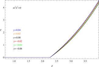
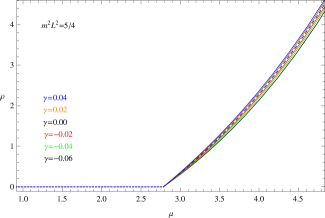
Figure 2: (color online) The charge density $\rho$ with respect to the chemical potential $\mu$ for different Weyl coupling parameters $\gamma$ with fixed masses of the vector field $m^{2}L^{2}=0$ (left) and $m^{2}L^{2}=5/4$ (right) in the holographic p-wave insulator and superconductor model. In each panel, the six lines from left to right correspond to decreasing $\gamma$, i.e., $0.04$ (blue), $0.02$ (orange), $0$ (black and dashed), $-0.02$ (red), $-0.04$ (green) and $\gamma=-0.06$ (black) respectively.

In Figs. 1 and 2 we plot the condensate of the vector operator $\langle J_{x}\rangle$ and charge density $\rho$ as a function of the chemical potential $\mu$ for different Weyl coupling parameters $\gamma$ with fixed masses of the vector field $m^{2}L^{2}=0$ (left) and $m^{2}L^{2}=5/4$ (right) in the holographic p-wave insulator and superconductor model. From Figs. 1 and 2, we find that the system is described by the AdS soliton solution itself when $\mu$ is small, which can be interpreted as the insulator phase Nishioka-Ryu-Takayanagi . However, there is a second order phase transition when $\mu\rightarrow\mu_{c}$ and the AdS soliton reaches the superconductor (or superfluid) phase for larger $\mu$. For the fixed Weyl coupling parameter $\gamma$, with the increase of the vector field mass, the critical chemical potential $\mu_{c}$ becomes larger. This property agrees well with the findings in the s-wave holographic insulator and superconductor model ZPJ2012 ; Pan-Wang . But for the fixed mass of the vector field, it is interesting to note that the critical chemical potential $\mu_{c}$ is independent of the Weyl coupling parameter $\gamma$, i.e.,

$$\mu_{c}=2.265,\quad{\rm for}~{}~{}m^{2}L^{2}=0~{}~{}{\rm and}~{}~{}\forall\gamma,$$

$$\mu_{c}=2.785,\quad{\rm for}~{}~{}m^{2}L^{2}=5/4~{}~{}{\rm and}~{}~{}\forall\gamma,$$ (11)

which shows that the Weyl couplings will not affect the properties of the holographic insulator/superconductor phase transition for the fixed mass of the vector field. This behavior is reminiscent of that seen for the holographic s-wave insulator/superconductor phase transition with Weyl corrections, but different from the holographic p-wave case with Weyl corrections via the Yang-Mills theory where the corrections do have effects on the insulator/superconductor phase transition ZPJ2012 . Thus, we conclude that the Weyl corrections have completely different effects on the critical chemical potential for the p-wave phase transitions of the Maxwell complex vector field model and that of the Yang-Mills theory.

II.2 Analytical understanding of holographic insulator/superconductor phase transition

Since the analytic Sturm-Liouville (S-L) method, which was first proposed by Siopsis and Therrien Siopsis and later generalized to study holographic insulator/superconductor phase transition in Cai-Li-Zhang , can clearly present the condensation and critical phenomena of the system at the critical point, we will apply it to investigate analytically the properties of holographic p-wave insulator/superconductor phase transition with Weyl corrections. In addition to back up numerical results, we will calculate analytically the critical exponent of the system at the critical point and obtain an analytical understanding in parallel.

Introducing the variable $z=r_{s}/r$, we can rewrite the equations of motion (5) and (6) into

$$\rho_{x}^{\prime\prime}+\left(\frac{1}{z}+\frac{f^{\prime}}{f}\right)\rho_{x}^{\prime}+\left(\frac{\phi^{2}}{z^{2}f}-\frac{m^{2}}{z^{4}f}\right)\rho_{x}=0\,,$$ (12)

$$(1+8\gamma z^{4})\phi^{\prime\prime}+\left[(1+40\gamma z^{4})\frac{1}{z}+(1+8\gamma z^{4})\frac{f^{\prime}}{f}\right]\phi^{\prime}-\frac{2\rho_{x}^{2}}{z^{2}f}\phi=0,$$ (13)

where the function $f$ now is $f(z)=(1-z^{4})/z^{2}$ and the prime denotes the derivative with respect to $z$.

At the critical chemical potential $\mu_{c}$, the vector field $\rho_{x}=0$. So below the critical point Eq. (13) reduces to

$$(1+8\gamma z^{4})\phi^{\prime\prime}+\left[(1+40\gamma z^{4})\frac{1}{z}+(1+8\gamma z^{4})\frac{f^{\prime}}{f}\right]\phi^{\prime}=0,$$ (14)

which results in a general solution

$$\phi=\mu+\frac{c_{1}}{4+32\gamma}\left[4\sqrt{2\gamma}{\rm ArcTan}(2\sqrt{2\gamma}z^{2})+\ln(1+z^{2})-\ln(1-z^{2})\right],$$ (15)

where $c_{1}$ is an integration constant. We see that the term in the square bracket is divergent at the tip $z=1$. Considering the Neumann-like boundary condition (II.1) for the gauge field $\phi$ at the tip $z=1$, we will set $c_{1}=0$ to keep $\phi$ finite, i.e., in this case $\phi$ has to be a constant. Thus, we can get the physical solution $\phi(z)=\mu$ to Eq. (14) if $\mu<\mu_{c}$, which agrees with our previous numerical results.

As $\mu\rightarrow\mu_{c}$ from below the critical point, the vector field equation (12) becomes

$$\rho_{x}^{\prime\prime}+\left(\frac{1}{z}+\frac{f^{\prime}}{f}\right)\rho_{x}^{\prime}+\left(\frac{\mu^{2}}{z^{2}f}-\frac{m^{2}}{z^{4}f}\right)\rho_{x}=0\,.$$ (16)

Obviously, the Weyl coupling parameter $\gamma$ is absent in the master Eq. (16) although Eq. (14) for the gauge field $\phi$ depends on $\gamma$, which leads that the Weyl corrections do not have any effect on the critical chemical potential $\mu_{c}$ for the fixed mass of the vector field, just as shown in Figs. 1 and 2.

Defining a trial function $F(z)$ near the boundary $z=0$ as Siopsis

$$\rho_{x}(z)\sim\langle J_{x}\rangle z^{\Delta_{+}}F(z),$$ (17)

with the boundary conditions $F(0)=1$ and $F^{\prime}(0)=0$, from Eq. (16) we can get the equation of motion for $F(z)$

$$(MF^{\prime})^{\prime}+M\left(U+\mu^{2}V\right)F=0,$$ (18)

where we have introduced

$$M=z^{2\Delta_{+}-1}(z^{4}-1),~{}~{}U=\frac{\Delta_{+}(\Delta_{+}-1)}{z^{2}}+\frac{\Delta_{+}}{z}\left(\frac{1}{z}+\frac{f^{\prime}}{f}\right)-\frac{m^{2}}{z^{4}f},~{}~{}V=\frac{1}{z^{2}f}.$$ (19)

Following the S-L eigenvalue problem Gelfand-Fomin , we obtain the expression which can be used to estimate the minimum eigenvalue of $\mu^{2}$

$$\mu^{2}=\frac{\int^{1}_{0}M\left(F^{\prime 2}-UF^{2}\right)dz}{\int^{1}_{0}MVF^{2}dz}=\frac{\Xi(a,m)}{\Sigma(a,m)},$$ (20)

with

$$\Xi(a,m) = \left(a-1\right)^{2}+\frac{1+m^{2}}{2\left(\Delta_{+}-1\right)}-\frac{am^{2}}{\Delta_{+}}+\frac{a^{2}\left(1+m^{2}\right)-1}{2\left(1+\Delta_{+}\right)}-\frac{a^{2}}{2\left(3+\Delta_{+}\right)},$$

$$\Sigma(a,m) = \frac{1}{2}\left[\frac{1}{\Delta_{+}}+a\left(\frac{a}{2+\Delta_{+}}-\frac{2}{1+\Delta_{+}}\right)\right],$$ (21)

where we have assumed the trial function to be $F(z)=1-az^{2}$ with a constant $a$ in the calculation. For different values of the mass of the vector field, we can get the minimum eigenvalue of $\mu^{2}$ and the corresponding value of $a$, for example, $\mu_{min}^{2}=7.768$ and $a=0.382$ for $m^{2}L^{2}=5/4$, which lead to the critical chemical potential $\mu_{c}=\mu_{min}=2.787$. In Table 1, we present the critical chemical potential $\mu_{c}$ for chosen mass of the vector field. Comparing with numerical results, we observe that the analytic results derived from S-L method are in very good agreement with the numerical computations.

Table 1: The critical chemical potential $\mu_{c}$ for the vector operator $\langle{J_{x}}\rangle$ obtained by the analytical S-L method and numerical shooting method with chosen various masses of the vector field for the holographic p-wave insulator/superconductor model. It should be noted that the Weyl corrections do not have any effect on $\mu_{c}$ for the fixed mass of the vector field.

$m^{2}L^{2}$	-1/2	-1/4	0	1/4	1/2	3/4	1	5/4
Analytical	$1.959$	$2.127$	$2.267$	$2.390$	$2.502$	$2.603$	$2.698$	$2.787$
Numerical	$1.958$	$2.125$	$2.265$	$2.388$	$2.500$	$2.601$	$2.696$	$2.785$

From Table 1, we find that, with the increase of the mass of the vector field, the critical chemical potential $\mu_{c}$ becomes larger, which agrees with our previous numerical results. More importantly, due to the absence of the Weyl coupling parameters from the master Eq. (16), the Weyl corrections do not have any effect on the critical chemical potential $\mu_{c}$ for the fixed mass of the vector field, which supports the numerical finding as shown in Figs. 1 and 2.

Now we are in a position to study the critical phenomena of this holographic p-wave system. Noting that the condensation of the vector operator $\langle J_{x}\rangle$ is so small when $\mu\rightarrow\mu_{c}$, we will expand $\phi(z)$ in small $\langle J_{x}\rangle$ as

$$\phi(z)\sim\mu_{c}+\langle J_{x}\rangle\chi(z)+\cdots,$$ (22)

where the boundary condition is $\chi(1)=0$ at the tip. Defining a function $\xi(z)$ as

$$\chi(z)=2\mu_{c}\langle J_{x}\rangle\xi(z),$$ (23)

we will have the equation of motion for $\xi(z)$

$$(K\xi^{\prime})^{\prime}-\frac{z^{2\Delta_{+}-3}(z^{4}-1)F^{2}}{f}=0,$$ (24)

with

$$K(z)=\frac{\left(z^{4}-1\right)\left(1+8\gamma z^{4}\right)}{z}.$$ (25)

According to the asymptotic behavior in Eq. (8), we can expand $\phi$ near $z\rightarrow 0$ as

$$\phi(z)\simeq\mu-\rho z^{2}\simeq\mu_{c}+\langle J_{x}\rangle\left[\chi(0)+\chi^{\prime}(0)z+\frac{1}{2}\chi^{\prime\prime}(0)z^{2}+\cdot\cdot\cdot\right].$$ (26)

From the coefficients of the $z^{0}$ term in both sides of the above formula and with the help of Eq. (23), we arrive at

$$\langle J_{x}\rangle=\frac{1}{\left[2\mu_{c}\xi(0)\right]^{\frac{1}{2}}}\left(\mu-\mu_{c}\right)^{\frac{1}{2}},$$ (27)

with

$$\xi(0)=c_{2}-\int^{1}_{0}\frac{1}{K(z)}\left[c_{3}+\int^{z}_{1}\frac{x^{2\Delta_{+}-3}F(x)^{2}(x^{4}-1)}{f(x)}dx\right]dz,$$ (28)

where the integration constants $c_{2}$ and $c_{3}$ can be determined by the boundary condition $\chi(z)$. For example, for the case of $\gamma=0.02$ with $m^{2}L^{2}=5/4$, we have $\langle J_{x}\rangle\approx 1.891(\mu-\mu_{c})^{1/2}$ when $a=0.382$, which agrees well with the numerical result given in the right panel of Fig. 1. Note that the expression (27) is valid for all cases considered here. Thus, the vector operator $\langle J_{x}\rangle$ satisfies $\langle J_{x}\rangle\sim(\mu-\mu_{c})^{1/2}$ near the critical point, which holds for various values of Weyl coupling parameters and masses of the vector field. The analytic result shows that the holographic p-wave insulator/superconductor phase transition belongs to the second order and the critical exponent of the system takes the mean-field value $1/2$, which can be used to back up the numerical findings obtained from Fig. 1.

Comparing the coefficients of the $z^{1}$ term in Eq. (26), we see that $\chi^{\prime}(0)\rightarrow 0$, which leads to $\xi^{\prime}(0)\rightarrow 0$. This behavior is consistent with the following relation by making integration of both sides of Eq. (24)

$$\left[\frac{\xi^{\prime}(z)}{z}\right]\bigg{|}_{z\rightarrow 0}=\int_{0}^{1}\frac{z^{2\Delta_{+}-3}(z^{4}-1)F^{2}}{f}dz.$$ (29)

Considering the coefficients of the $z^{2}$ term in Eq. (26), we get

$$\rho=-\frac{1}{2}\langle J_{x}\rangle\chi^{\prime\prime}(0)=\Gamma(\gamma,m)(\mu-\mu_{c}),$$ (30)

with

$$\Gamma(\gamma,m)=-\frac{1}{2\xi(0)}\int_{0}^{1}\frac{z^{2\Delta_{+}-3}(z^{4}-1)F^{2}}{f}dz,$$ (31)

which is a function of the Weyl coupling parameter and the vector field mass. For the case of $\gamma=0.02$ with $m^{2}L^{2}=5/4$, as an example, we can find $\rho=1.068\left(\mu-\mu_{c}\right)$ when $a=0.382$, which is in good agreement with the result shown in the right panel of Fig. 2. Since the Weyl coupling parameters and masses of the vector field will not alter Eq. (30), we can obtain the linear relation between the charge density and the chemical potential near $\mu_{c}$, i.e., $\rho\sim(\mu-\mu_{c})$, which supports the numerical result presented in Fig. 2.

III p-wave superconductor models with Weyl corrections in AdS black hole

Since the Weyl couplings will not affect the properties of the new p-wave superconductor in AdS soliton via the Maxwell complex vector field model, which is different from that via the Yang-Mills theory where the Weyl corrections do have effects on the insulator/superconductor phase transition, it seems to be an interesting study to consider the influences of the Weyl corrections on this new p-wave superconductor in AdS black hole.

III.1 Numerical investigation of holographic metal/superconductor phase transition

In the probe limit, the background metric is a five-dimensional planar Schwarzschild-AdS black hole

$$ds^{2}=-f\left(r\right)dt^{2}+\frac{1}{f\left(r\right)}dr^{2}+r^{2}\left(dx^{2}+dy^{2}+dz^{2}\right),$$ (32)

where $f(r)=r^{2}(1-r_{+}^{4}/r^{4})$ with the radius of the event horizon $r_{+}$. The Hawking temperature of the black hole can be expressed as

$$T=\frac{r_{+}}{\pi},$$ (33)

which can be interpreted as the temperature of the CFT. The metric (32) has the following nonzero components of the Weyl tensor $C_{\mu\nu\rho\sigma}$

$$C_{0i0j}=\frac{r_{+}^{4}f\left(r\right)}{r^{2}}\delta_{ij},\quad C_{0r0r}=-\frac{3r_{+}^{4}}{r^{4}},\quad C_{irjr}=-\frac{r_{+}^{4}}{r^{2}f\left(r\right)}\delta_{ij},\quad C_{ijkl}=r_{+}^{4}\delta_{ik}\delta_{jl},$$ (34)

with $i,~{}j,~{}k,~{}l=x$, $y$ or $z$.

For completeness, we still work on the ansatz (4) and get the equations of motion from the action (1) in the Maxwell complex vector field model

$$\rho_{x}^{\prime\prime}+\left(\frac{1}{r}+\frac{f^{\prime}}{f}\right)\rho_{x}^{\prime}+\left(\frac{q^{2}\phi^{2}}{f^{2}}-\frac{m^{2}}{f}\right)\rho_{x}=0\,,$$ (35)

$$\left(1-\frac{24\gamma r_{+}^{4}}{r^{4}}\right)\phi^{\prime\prime}+\frac{3}{r}\left(1+\frac{8\gamma r_{+}^{4}}{r^{4}}\right)\phi^{\prime}-\frac{2q^{2}\rho_{x}^{2}}{r^{2}f}\phi=0,$$ (36)

where the prime denotes the derivative with respect to $r$.

In order to solve the equations of motion (35) and (36) numerically, we have to impose the appropriate boundary conditions for $\rho_{x}(r)$ and $\phi(r)$. At the horizon $r=r_{+}$, the boundary conditions are

$$\rho_{x}(r_{+})=\frac{f^{\prime}(r_{+})}{m^{2}}\rho_{x}^{\prime}(r_{+})\,,\hskip 14.22636pt\phi(r_{+})=0\,.$$ (37)

Obviously, we require $\phi\left(r_{+}\right)=0$ in order for $g^{\mu\nu}A_{\mu}A_{\nu}$ to be finite at the horizon, which is in strong contrast to that of the AdS soliton where there is a constant nonzero gauge field $\phi(r_{s})$ at $r=r_{s}$. But near the boundary $r\rightarrow\infty$, we find that the solutions have the same boundary conditions just as Eq. (8) for the holographic p-wave insulator and superconductor model with Weyl corrections.

For the equations of motion (35) and (36), we can also obtain the useful scaling symmetries

$$r\rightarrow\alpha r\,,\hskip 14.22636pt(t,x,y,z)\rightarrow\frac{1}{\alpha}(t,x,y,z)\,,\hskip 14.22636pt(\rho_{x},\phi)\rightarrow\alpha(\rho_{x},\phi)\,,\hskip 14.22636pt$$ (38)

which result in the transformation of the relevant quantities

$$T\rightarrow\alpha T\,,\hskip 14.22636pt\mu\rightarrow\alpha\mu\,,\hskip 14.22636pt\rho\rightarrow\alpha^{3}\rho\,,\hskip 14.22636pt\rho_{x+}\rightarrow\alpha^{1+\Delta_{+}}\rho_{x+}\,,\hskip 14.22636pt$$ (39)

with a real positive number $\alpha$. Without loss of generality, we can scale $r_{+}=1$ and set $q=1$ in the following just as in CaiPWave-1 .

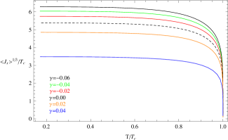
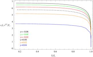
Figure 3: (color online) The condensate of the operator $\langle J_{x}\rangle=\rho_{x+}$ as a function of temperature for different Weyl coupling parameters $\gamma$ with fixed masses of the vector field $m^{2}L^{2}=0$ (left) and $m^{2}L^{2}=5/4$ (right) in the holographic p-wave superconductor model. In each panel, the six lines from top to bottom correspond to increasing $\gamma$, i.e., $\gamma=-0.06$ (black), $-0.04$ (green), $-0.02$ (red), $0$ (black and dashed), $0.02$ (orange) and $0.04$ (blue) respectively.

In Fig. 3, we present the condensate of the vector operator $\langle J_{x}\rangle$ as a function of temperature for different Weyl coupling parameters $\gamma$ with fixed masses of the vector field $m^{2}L^{2}=0$ (left) and $m^{2}L^{2}=5/4$ (right) in the holographic p-wave superconductor model. Obviously, we observe that the behavior of each curve for the fixed $\gamma$ and $m^{2}L^{2}$ is in good agreement with the holographic superconducting phase transition in the literature, which shows that the black hole solution with non-trivial vector field can describe a superconducting phase.

From Fig. 3, for the fixed Weyl coupling parameter $\gamma$, we find that the condensation gap for the vector operator $\langle J_{x}\rangle$ becomes larger with the increase of the mass of the vector field, which implies that the increase of the mass makes it harder for the vector operator to condense. However, if we concentrate on the same mass of the vector field, we see that the higher correction term $\gamma$ makes the condensation gap smaller, which means that the condensation is easier to be formed when the parameter $\gamma$ increases. In fact, the table 2 shows that the critical temperature $T_{c}$ for the vector operator $\langle J_{x}\rangle$ with the fixed vector field mass increases as the correction term $\gamma$ increases, which agrees well with the finding in Fig. 3. This behavior is reminiscent of that seen for the holographic p-wave dual models via the Yang-Mills theory, where the critical temperature $T_{c}$ increases as the Weyl correction $\gamma$ increases MomeniSL . So we conclude that these two p-wave models with Weyl corrections share some similar features for the condensation of the vector operator.

Table 2: The critical temperature $T_{c}$ obtained by the numerical shooting method for the vector operator $\langle J_{x}\rangle$ with different Weyl coupling parameters $\gamma$ and fixed masses of the vector field, i.e., $m^{2}L^{2}=0$ and $5/4$. We have set $\rho=1$ in the table.

$\gamma$	-0.06	-0.04	-0.02	0	0.02	0.04
$m^{2}L^{2}=0$	$0.172$	$0.179$	$0.188$	$0.201$	$0.222$	$0.309$
$m^{2}L^{2}=5/4$	$0.157$	$0.163$	$0.172$	$0.184$	$0.205$	$0.288$

III.2 Analytical understanding of holographic metal/superconductor phase transition

We still use the S-L method to deal with the effect of the Weyl corrections on the holographic p-wave metal/superconductor phase via the Maxwell complex vector field model. Changing the coordinate and setting $z=r_{+}/r$, we can convert the equations of motion (35) and (36) to be

$$\rho_{x}^{\prime\prime}+\left(\frac{1}{z}+\frac{f^{\prime}}{f}\right)\rho_{x}^{\prime}+\frac{1}{z^{4}}\left(\frac{\phi^{2}}{r_{+}^{2}f^{2}}-\frac{m^{2}}{f}\right)\rho_{x}=0\,,$$ (40)

$$\left(1-24\gamma z^{4}\right)\phi^{\prime\prime}-\left(\frac{1}{z}+72\gamma z^{3}\right)\phi^{\prime}-\frac{2\rho_{x}^{2}}{r_{+}^{2}z^{2}f}\phi=0.$$ (41)

Here the function $f$ has been rewritten into $f(z)=(1-z^{4})/z^{2}$ and the prime denotes the derivative with respect to $z$.

At the critical temperature $T_{c}$, the vector field $\rho_{x}=0$. Thus, below the critical point Eq. (41) becomes

$$\left(1-24\gamma z^{4}\right)\phi^{\prime\prime}-\left(\frac{1}{z}+72\gamma z^{3}\right)\phi^{\prime}=0.$$ (42)

Note that at $z=0$, from the boundary condition we have

$$\phi^{\prime\prime}|_{z=0}=-\frac{2\rho}{r_{+}^{2}}\quad{\rm at}~{}~{}T=T_{c}.$$ (43)

Thus, neglecting terms of order $0(\gamma^{n\geq 2})$, we can obtain the solution to Eq. (42)

$$\phi(z)=\lambda r_{+}\varphi_{1}(z)=\lambda r_{+}\left(1-z^{2}\right)\left[1+8\gamma\left(1+z^{2}+z^{4}\right)\right],$$ (44)

with $\lambda=\rho/r_{+}^{3}$.

Near the boundary $z=0$, we introduce a trial function $F(z)$

$$\rho_{x}|\sim\frac{\langle J_{x}\rangle}{r_{+}^{\Delta_{+}}}z^{\Delta_{+}}F(z),$$ (45)

with the boundary conditions $F(0)=1$ and $F^{\prime}(0)=0$. Therefore the equation of motion for $F(z)$ is given by

$$(MF^{\prime})^{\prime}+M\left(P+\lambda^{2}Q\right)F=0,$$ (46)

with

$$P=\frac{\Delta_{+}}{z}\left(\frac{\Delta_{+}}{z}+\frac{f^{\prime}}{f}\right)-\frac{m^{2}}{z^{4}f},~{}~{}Q=\frac{\varphi_{1}^{2}}{z^{4}f^{2}},$$ (47)

where $M(z)$ has been defined in (19). According to the S-L eigenvalue problem Gelfand-Fomin , we deduce the eigenvalue $\lambda$ minimizes the expression

$$\lambda^{2}=\frac{\int^{1}_{0}M\left(F^{\prime 2}-PF^{2}\right)dz}{\int^{1}_{0}MQF^{2}dz}.$$ (48)

Here we still assume the trial function to be $F(z)=1-az^{2}$ with a constant $a$. Using above equation to compute the minimum eigenvalue of $\lambda^{2}$, we can get the critical temperature $T_{c}$ for different Weyl coupling parameters $\gamma$ and masses of the vector field $m$ from the following relation

$$T_{c}=\frac{1}{\pi\lambda_{min}^{1/3}}\sqrt[3]{\rho}.$$ (49)

As an example, for the case of $m^{2}L^{2}=5/4$ with the chosen value of the Weyl coupling parameter $\gamma=0.02$, we obtain the minimum $\lambda_{min}=18.069$ at $a=0.748$. According to the relation (49), we can easily get the critical temperature $T_{c}=0.196\sqrt[3]{\rho}$, which is consistent with the numerical result $T_{c}=0.205\sqrt[3]{\rho}$ in Table 2. In Table 3 we give the critical temperature $T_{c}$ obtained by the analytical S-L method for the vector operator $\langle J_{x}\rangle$ when we fix the mass of the vector field $m^{2}L^{2}$ for different Weyl couplings by choosing the expanded solution (44) upto first order in the Weyl coupling parameter. Comparing with the numerical results of Table 2 in the range $-0.02\leq\gamma\leq 0.02$, we observe that the differences between the analytical and numerical values are within $4.5\%$.

Table 3: The critical temperature $T_{c}$ obtained by the analytical S-L method for the vector operator $\langle J_{x}\rangle$ with different Weyl coupling parameters $\gamma$ and fixed masses of the vector field, i.e., $m^{2}L^{2}=0$ and $5/4$. We have set $\rho=1$ and chosen different expanded solutions to Eq. (42), i.e., $\varphi_{1}$ upto $0(\gamma)$ and $\varphi_{2}$ upto $0(\gamma^{6})$ in the table.

$\gamma$	-0.02	-0.01	0	0.01	0.02
$m^{2}L^{2}=0~{}~{}(\varphi_{1})$	$0.181$	$0.190$	$0.199$	$0.207$	$0.214$
$m^{2}L^{2}=0~{}~{}(\varphi_{2})$	$0.186$	$0.192$	$0.199$	$0.208$	$0.221$
$m^{2}L^{2}=5/4~{}~{}(\varphi_{1})$	$0.165$	$0.174$	$0.182$	$0.189$	$0.196$
$m^{2}L^{2}=5/4~{}~{}(\varphi_{2})$	$0.169$	$0.175$	$0.182$	$0.191$	$0.203$

When we perform analytic computation of the solution to Eq. (42) upto sixth order in the Weyl coupling parameter $\gamma$, i.e., change the solution (44) into

$$\phi(z) = \lambda r_{+}\varphi_{2}(z)$$

$$= \lambda r_{+}\left[\varphi_{1}(z)+\frac{24^{2}}{5}(1-z^{10})\gamma^{2}+\frac{24^{3}}{7}(1-z^{14})\gamma^{3}+\frac{24^{4}}{9}(1-z^{18})\gamma^{4}+\frac{24^{5}}{11}(1-z^{22})\gamma^{5}+\frac{24^{6}}{13}(1-z^{26})\gamma^{6}\right],$$

the agreement of the analytic results presented in Table 3 with the numerical calculation shown in Table 2 is impressive. Thus, we can improve the analytic result and get the critical temperature more consistent with the numerical result if we expand the solution to Eq. (42) upto a sufficiently high order in the Weyl coupling parameter $\gamma$, even we consider the case of larger $\gamma$.

From Table 3, we point out that the critical temperature $T_{c}$ increases as the Weyl correction $\gamma$ increases for the fixed vector field mass but decreases as the mass $m^{2}$ increases for the fixed Weyl coupling parameter, which supports the numerical computation shown in Fig. 3 and Table 2.

We will investigate the critical phenomena of the system. Since the condensation for the vector operator $\langle J_{x}\rangle$ is so small when $T\rightarrow T_{c}$, we can expand $\phi(z)$ in $\langle J_{x}\rangle$ near $z=0$

$$\frac{\phi(z)}{r_{+}}=\lambda\varphi_{1}+\frac{\langle J_{x}\rangle^{2}}{r_{+}^{2(1+\Delta_{+})}}\chi\left(z\right)+\cdot\cdot\cdot,$$ (51)

with the boundary conditions $\chi(1)=0$ and $\chi^{\prime}(1)=0$ Siopsis ; Li-Cai-Zhang . Thus, substituting the functions (45) and (51) into (41), we can get the equation of motion for $\chi\left(z\right)$

$$\left(W\chi^{\prime}\right)^{\prime}-\frac{2\lambda z^{2\Delta_{+}-3}F^{2}\varphi_{1}}{f}=0,$$ (52)

where we have introduced a new function

$$W(z)=\frac{1-24\gamma z^{4}}{z}.$$ (53)

From the asymptotic behavior (8), near $z\rightarrow 0$ we can arrive at

$$\frac{\phi(z)}{r_{+}} = \frac{\rho}{r^{3}_{+}}(1-z^{2})$$ (54)

$$= \lambda\left(1-z^{2}\right)\left[1+8\gamma\left(1+z^{2}+z^{4}\right)\right]+\frac{\langle J_{x}\rangle^{2}}{r_{+}^{2(1+\Delta_{+})}}\left[\chi(0)+\chi^{\prime}(0)z+\frac{1}{2}\chi^{\prime\prime}(0)z^{2}+\cdot\cdot\cdot\right].$$

Considering the coefficients of the $z^{1}$ term in both sides of the above formula, we can find that $\chi^{\prime}(0)\rightarrow 0$, which agrees well with the following relation by making integration of both sides of Eq. (52)

$$\left[\frac{\chi^{\prime}(z)}{z}\right]\bigg{|}_{z\rightarrow 0}=-2\lambda\Upsilon(\gamma,m)=-2\lambda\int_{0}^{1}\frac{z^{2\Delta_{+}-3}F^{2}\varphi_{1}}{f}dz,$$ (55)

where $\Upsilon(\gamma,m)$ is a function of the Weyl coupling parameter and the vector field mass. Comparing the coefficients of the $z^{2}$ term in Eq. (54), we have

$$\frac{\rho}{r^{3}_{+}}=\lambda-\frac{\langle J_{x}\rangle^{2}}{2r_{+}^{2(1+\Delta_{+})}}\chi^{\prime\prime}(0),$$ (56)

which leads to

$$\langle J_{x}\rangle=\left(\pi T_{c}\right)^{1+\Delta_{+}}\sqrt{\frac{3}{\Upsilon(\gamma,m)}}\left(1-\frac{T}{T_{c}}\right)^{\frac{1}{2}}.$$ (57)

Obviously, the expression (57) is valid for all cases considered here. For example, for the case of $\gamma=0.02$ with $m^{2}L^{2}=5/4$, we have $\langle J_{x}\rangle\approx 1.580(1-T/T_{c})^{1/2}$ when $a=0.748$, which is in agreement with the numerical calculation given in the right panel of Fig. 3. Since the Weyl coupling parameters and masses of the vector field will not alter Eq. (57) except for the prefactor, we can obtain the relation $\langle J_{x}\rangle\sim(1-T/T_{c})^{1/2}$ near the critical point. The analytic result shows that the holographic p-wave metal/superconductor phase transition belongs to the second order and the critical exponent of the system takes the mean-field value $1/2$, which can be used to back up the numerical findings shown in Fig. 3.

IV Conclusions

In the probe limit, we have investigated the holographic p-wave dual models with Weyl corrections both in the backgrounds of AdS soliton and AdS black hole in order to understand the influences of the $1/N$ or $1/\lambda$ corrections on the vector condensate via a Maxwell complex vector field model. Different from the holographic p-wave insulator/superconductor models in the Yang-Mills theory, we found in the AdS soliton background that the critical chemical potentials are independent of the Weyl correction term, which tells us that the correction to the Maxwell field will not affect the properties of this new holographic p-wave insulator/superconductor phase transition. We also observed that the effect of the Weyl corrections cannot modify the critical phenomena, and found that this new insulator/superconductor phase transition belongs to the second order and the critical exponent of the system always takes the mean-field value $1/2$. We confirmed our numerical result by using the S-L analytic method and concluded that the Weyl corrections have different effects on the holographic p-wave insulator/superconductor phase transition of the Maxwell complex vector field model and that of the Yang-Mills theory.

However, the story is completely different if we study the holographic p-wave metal/superconductor phase transition with Weyl corrections. We observed that similar to the effect of the Weyl corrections in the Yang-Mills theory, in the black hole background, the critical temperature for the vector operator increases as the correction term increases, which implies that the higher Weyl corrections make it easier for the vector condensation to form. Further analytic studies showed that the holographic p-wave metal/superconductor phase transition belongs to the second order and the critical exponent of the system takes the mean-field value $1/2$, which supports our numerical findings. Comparing the holographic p-wave metal/superconductor phase transitions of the Maxwell complex vector field model with that of the Yang-Mills theory, we argued that these two p-wave models with Weyl corrections share some similar features for the condensation of the vector operator.

References

• (1) J. Maldacena, Adv. Theor. Math. Phys. 2, 231 (1998) [Int. J. Theor. Phys. 38, 1113 (1999)].
• (2) S.S. Gubser, Phys. Rev. D 78, 065034 (2008).
• (3) S.A. Hartnoll, C.P. Herzog, and G.T. Horowitz, Phys. Rev. Lett. 101, 031601 (2008).
• (4) S.A. Hartnoll, C.P. Herzog, and G.T. Horowitz, J. High Energy Phys. 12, 015 (2008).
• (5) T. Nishioka, S. Ryu, and T. Takayanagi, J. High Energy Phys. 03, 131 (2010).
• (6) S.A. Hartnoll, Class. Quant. Grav. 26, 224002 (2009).
• (7) C.P. Herzog, J. Phys. A 42, 343001 (2009).
• (8) G.T. Horowitz, Lect. Notes Phys. 828 313, (2011); arXiv:1002.1722 [hep-th].
• (9) R. Gregory, S. Kanno, and J. Soda, J. High Energy Phys. 10, 010 (2009).
• (10) Q.Y. Pan, B. Wang, E. Papantonopoulos, J. Oliveira, and A.B. Pavan, Phys. Rev. D 81, 106007 (2010).
• (11) J.L. Jing and S.B. Chen, Phys. Lett. B 686, 68 (2010).
• (12) J.P. Wu, Y. Cao, X.M. Kuang, and W.J. Li, Phys. Lett. B 697, 153 (2011).
• (13) D. Momeni, N. Majd, and R. Myrzakulov, Europhys. Lett. 97, 61001 (2012).
• (14) Z.X. Zhao, Q.Y. Pan, and J.L. Jing, Phys. Lett. B 719, 440 (2013); arXiv:1212.3062 [hep-th].
• (15) D.Z. Ma, Y. Cao, and J.P. Wu, Phys. Lett. B 704, 604 (2011).
• (16) D. Momeni and M.R. Setare, Mod. Phys. Lett. A 26, 2889 (2011).
• (17) D. Roychowdhury, Phys. Rev. D 86, 106009 (2012).
• (18) D. Momeni, M.R. Setare, and R. Myrzakulov, Int. J. Mod. Phys. A 27, 1250128 (2012).
• (19) D. Momeni, R. Myrzakulov, and M. Raza, Int. J. Mod. Phys. A 28, 1350096 (2013).
• (20) L.C. Zhang, H.F. Li, H.H. Zhao, and R. Zhao, Int. J. Theor. Phys. 52, 2455 (2013).
• (21) D. Momeni, M. Raza, and R. Myrzakulov, arXiv:1410.8379 [hep-th].
• (22) R.G. Cai, S. He, L. Li, and L.F. Li, J. High Energy Phys. 12, 036 (2013); arXiv:1309.2098 [hep-th].
• (23) R.G. Cai, L. Li, and L.F. Li, J. High Energy Phys. 01, 032 (2014); arXiv:1309.4877 [hep-th].
• (24) L.F. Li, R.G. Cai, L. Li, and C. Shen, arXiv:1310.6239 [hep-th].
• (25) R.G. Cai, L. Li, L.F. Li, and Y. Wu, J. High Energy Phys. 01, 045 (2014); arXiv:1311.7578 [hep-th].
• (26) R.G. Cai, L. Li, L.F. Li, and R.Q. Yang, J. High Energy Phys. 04, 016 (2014); arXiv:1401.3974 [gr-qc].
• (27) Y.B. Wu, J.W. Lu, M.L. Liu, J.B. Lu, C.Y. Zhang, and Z.Q. Yang, Phys. Rev. D 89, 106006 (2014); arXiv:1403.5649 [hep-th].
• (28) Y.B. Wu, J.W. Lu, Y.Y. Jin, J.B. Lu, X. Zhang, S.Y. Wu, and C. Wang, Int. J. Mod. Phys. A 29, 1450094 (2014); arXiv:1405.2499 [hep-th].
• (29) R.G. Cai and R.Q. Yang, Phys. Rev. D 91, 026001 (2015); arXiv:1410.5080 [hep-th].
• (30) Y.B. Wu, J.W. Lu, W.X. Zhang, C.Y. Zhang, J.B. Lu, and F. Yu, Phys. Rev. D 90, 126006 (2014); arXiv:1410.5243 [hep-th].
• (31) Y.B. Wu, J.W. Lu, C.Y. Zhang, N. Zhang, X. Zhang, Z.Q. Yang, S.Y. Wu, Phys. Lett. B 741, 138 (2015); arXiv:1412.3689 [hep-th].
• (32) A. Ritz and J. Ward, Phys. Rev. D 79, 066003 (2009); arXiv:0811.4195 [hep-th].
• (33) G. Siopsis and J. Therrien, J. High Energy Phys. 05, 013 (2010).
• (34) R.G. Cai, H.F. Li, and H.Q. Zhang, Phys. Rev. D 83, 126007 (2011); arXiv:1103.5568 [hep-th].
• (35) I.M. Gelfand and S.V. Fomin, Calculus of Variations, Revised English Edition, Translated and Edited by R.A. Silverman, Prentice-Hall, Inc. Englewood Cliff, New Jersey (1963).
• (36) H.F. Li, R.G. Cai, and H.Q. Zhang, J. High Energy Phys. 04, 028 (2011); arXiv:1103.2833 [hep-th].