Non-perturbative studies of $\mathcal{N}=2$ conformal

quiver gauge theories

S. K. Ashok¹, M. Billó², E. Dell’Aquila¹, M. Frau², R. R. John¹, A. Lerda<sup>2

1</sup>Institute of Mathematical Sciences,
C.I.T. Campus, Taramani
Chennai, India 600113

² Università di Torino, Dipartimento di Fisica
and I.N.F.N. - sezione di Torino
Via P. Giuria 1, I-10125 Torino, Italy
sashok,edellaquila,renjan@imsc.res.in,
billo,frau,lerda@to.infn.it

We study ${\mathcal{N}}=2$ super-conformal field theories in four dimensions that correspond to mass-deformed linear quivers with $n$ gauge groups and (bi-)fundamental matter. We describe them using Seiberg-Witten curves obtained from an M-theory construction and via the AGT correspondence. We take particular care in obtaining the detailed relation between the parameters appearing in these descriptions and the physical quantities of the quiver gauge theories. This precise map allows us to efficiently reconstruct the non-perturbative prepotential that encodes the effective IR properties of these theories. We give explicit expressions in the cases $n=1,2$, also in the presence of an $\Omega$-background in the Nekrasov-Shatashvili limit. All our results are successfully checked against those of the direct microscopic evaluation of the prepotential à la Nekrasov using localization methods.

Dedicated to the memory of Tullio Regge

1 Introduction and summary

Superconformal field theories (SCFT) with ${\mathcal{N}}=2$ supersymmetry in four dimensions have attracted a lot of attention, and tremendous progress has been made in describing them and in uncovering their duality structure [1]. Various approaches have been pursued: the geometric description of the low-energy effective action à la Seiberg-Witten (SW) [2, 3], the exact computation of instanton corrections by means of localization techniques [4, 5], the relations to integrable models [6], the 2d/4d correspondence also known as the AGT correspondence [7, 8], the use of $\beta$-ensembles and matrix model techniques [9, 10]. Moreover, the string embedding of such theories via geometric engineering has led to the possibility of expressing some relevant observables via topological string amplitudes [11]-[13], and further insights have been obtained by considering several aspects of the gauge/gravity relation and holography in this context [19]-[30] . The profound interplay among these various approaches is one of the most fruitful lessons to be learned from studying ${\mathcal{N}}=2$ SCFT’s. Let us emphasize that this interplay relies crucially on the precise relation between the parameters used in the various approaches, uncovered and verified through the analysis of examples of increasing complexity. This is the main rationale behind the work we present here.

From a purely gauge-theoretic point of view, mass-deformed conformal quiver theories have been studied in [31]-[33] through limit-shape equations obtained from the saddle-point analysis [34] of Nekrasov partition functions. This has led to a deeper understanding of the SW geometry of conformal gauge theories and it has clarified the relation between gauge theories, integrable systems and the quantization of various moduli spaces. Our goal in this work is more pragmatic: we discuss and compare various approaches available to study the conformal quiver theories, find the detailed map between the parameters that appear in these approaches, and propose an efficient way to calculate the prepotential of the gauge theory.

A particularly simple class of ${\mathcal{N}}=2$ SCFT’s are those of the so-called class ${\mathcal{S}}$ [1], which arise as compactifications of a $(2,0)$ 6-dimensional theory and admit various weakly-coupled descriptions related by S-dualities. Each of these descriptions contains products of $\mathrm{SU}(N_{i})$ gauge groups plus matter arranged in representations such that all $\beta$-functions vanish. Here we will focus on class ${\mathcal{S}}$ theories that have a weak-coupling realization in terms of linear quivers with $n$ SU(2) gauge groups and matter in fundamental or bi-fundamental representations. For these theories one can apply localization techniques [4, 5] to compute microscopically the prepotential $F$ as an expansion in powers of the instanton weights $q_{i}$, with coefficients depending on the masses and on the eigenvalues $a_{i}$ of the vacuum expectation value $\langle\Phi_{i}\rangle$ of the adjoint scalar of the $i$-th gauge group. In Appendix A we briefly describe this computation and give the expression of the non-perturbative prepotential for the first few instanton numbers. These explicit results provide a very concrete testing ground for any description of the IR regime of these theories.

Localization computations require the introduction of the $\Omega$-deformation parameters $\epsilon_{1}$ and $\epsilon_{2}$, which encode an explicit breaking of the SO(4) Euclidean space-time symmetry. The logarithm of the resulting partition function describes the prepotential $F$ in the limit $\epsilon_{1,2}\to 0$, plus a series of $\epsilon$-corrections which correspond to deformations of the gauge theory in the presence of constant backgrounds for bulk fields, like for example the graviphoton [39, 40]. The study of such $\epsilon$-deformations represents an important line of research, and various methods have been used to tackle it [41]-[43].

In this paper we will consider two distinct approaches to the study of linear quivers: first, we study the IR description of the SU(2)ⁿ theories using the SW curve obtained via an M-theory construction [44]; next, we use the AGT correspondence [7, 8] and analyze chiral conformal blocks of Liouville theory in two dimensions. We then show that these two approaches are equivalent to the microscopic multi-instanton calculations of Nekrasov. To this end, we need all observables, whether arising from M-theory or from the Liouville theory, to be expressed in terms of the physical masses and bare coupling constants of the gauge theory. Therefore we work out the precise and explicit map between the geometric parameters of M-theory, the parameters of the Liouville conformal field theory and the physical parameters of the gauge theory.

Let us now briefly describe the content of this paper. We begin with the SW curve description of the quiver theories. In general, for class ${\mathcal{S}}$ theories the SW curves cover a base $C$ which is a Riemann surface with marked punctures whose positions parametrize the moduli space of the marginal UV gauge couplings. For the quiver theories we consider, $C$ is a sphere with $(n+3)$ punctures and the expression of the SW curve and of the corresponding SW differential $\lambda$ can be derived starting from a NS5-D4 system uplifted to M-theory, as originally shown in [44] and studied in great detail in [1, 45]. In Section 2 we revisit this procedure for a generic quiver with $n$ nodes and derive explicitly the curves for generic $n$ in the massless case and for $n=1,2$ in the presence of masses. These curves are of the form [1]:

$$x^{2}(t)=\frac{{\mathcal{P}}_{2n+2}(t)}{t^{2}(t-t_{1})^{2}\cdots(t-t_{n})^{2}(t-1)^{2}}~{},$$ (1.1)

where the $t_{i}$’s are the positions of the punctures which are related to the gauge theory couplings as $q_{i}=t_{i}/t_{i+1}$, while ${\mathcal{P}}_{2n+2}(t)$ is a polynomial of degree $(2n+2)$ which depends on the $q_{i}$’s, on the masses and on the Coulomb branch parameters $u_{i}$. If we are to check the curve (1.1) against the microscopic prepotential $F$, we have to take into account the fact that the prepotential depends on the eigenvalues $a_{i}$. In the SW approach, the variables $a_{i}$ and their duals $a_{i}^{D}=\partial F/\partial a_{i}$ correspond to periods of the differential $\lambda$ over a symplectic basis of cycles on the SW curve, and are thus functions of the parameters $u_{i}$ appearing in (1.1). By inverting the functions $a_{i}(u)$ to express $u_{i}$ in terms of $a_{i}$, we can recast the dual periods $a_{i}^{D}(u)$ as functions of $a_{i}$ and hence compute the IR couplings $\tau_{ij}=\partial a_{i}^{D}/\partial a_{j}=\partial^{2}F/(\partial a_{i}\partial a_{j})$. Integrating this formula twice we obtain $F$ as a function of the $a_{i}$’s, and we can then compare it with the Nekrasov prepotential.

This procedure is in practice rather cumbersome, just because the integrals leading to the dual periods $a_{i}^{D}$ are often difficult to compute. Various strategies have been developed to reconstruct the prepotential from the SW curve avoiding the direct computation of the dual periods. A central rôle in these strategies is played by relations of the Matone type [46] which, in the class of theories we study, take the form

$$U_{i}=q_{i}\frac{\partial F}{\partial q_{i}}~{},$$ (1.2)

where $U_{i}=\langle\mathrm{Tr}\,\Phi_{i}^{2}\rangle$ is the gauge-invariant modulus of the $i$-th gauge group. If we know the relation between the parameters $u_{i}$’s appearing in the curve and the physical moduli $U_{i}$’s, after inverting the periods $a_{i}$ as discussed above, we can directly obtain the $U_{i}$’s as functions of the $a_{i}$’s and obtain the prepotential $F$ by integrating once the Matone-like relations with respect to (the logarithm of) the $q_{i}$’s.

In recent works [47, 48], it has been proposed that the $U_{i}$’s should be identified with the residues of the quadratic differential $x^{2}(t)$ at the various punctures of the SW curve; this identification yields an explicit map from the $u_{i}$’s (appearing in $x^{2}(t)$) to the $U_{i}$’s, thereby allowing for an efficient computation of the prepotential. We show that in the mass-deformed theory, global symmetries of the quiver theory play a crucial role in deriving the precise relation between the residues of $x^{2}(t)$ and the prepotential of the gauge theory. Having done this, we explicitly compute in Sections 3 and 4 the periods $a_{i}$ in the cases $n=1$ and $n=2$, and then reconstruct $F$. The prepotential we obtain in this way perfectly agrees with the microscopic results, presented in Appendix A.

We also perform another consistency check on the SW description of the linear quiver, which provides interesting relations between the UV and the IR parameters of the gauge theory. If we consider the hyperelliptic form of the SW curve, $y^{2}={\mathcal{P}}_{2n+2}(t)$, the classical Thomæ formulæ [49, 50] express the cross-ratios of the roots of the polynomial ${\mathcal{P}}_{2n+2}$ in terms of Riemann $\Theta$-constants at genus $n$. These are constructed in terms of the period matrix $\tau_{ij}$ which represents the matrix of low-energy effective couplings of the gauge theory and can be computed from the prepotential. We show that the Thomæ formulæ do indeed yield the cross-ratios of the roots of ${\mathcal{P}}_{2n+2}$, provided we relate the parameters $u_{i}$ appearing in ${\mathcal{P}}_{2n+2}$ to the moduli $U_{i}$ exactly as required by the residue prescription discussed above. Thus, even if we did not assume this prescription, we would be led to it by this analysis. We also note that, in the massless case, the cross-ratios of the roots of ${\mathcal{P}}_{2n+2}$ are just the UV couplings $q_{i}$, so the Thomæ formulæ express the UV couplings in terms of the IR couplings $\tau_{ij}$ as rational functions of Riemann $\Theta$-constants; in the SU(2) theory with $N_{f}=4$, these formulæ reduce to the well-known relation $q=\theta_{4}(\tau)^{4}/\theta_{2}(\tau)^{4}$ [51].

In Sections 5 and 6 we then turn to the corrections to the prepotential induced by the $\Omega$-deformation. For this purpose we use the well-established AGT correspondence [7] for the conformal $\mathrm{SU(2)}^{n}$ quivers. In particular, we work in the Nekrasov-Shatashvili (NS) limit, where one sets $\epsilon_{2}=0$, and show that in this limit the SW curve and the $\epsilon_{1}$-deformed SW differential appear naturally in the analysis of a null-vector decoupling equation satisfied by a conformal block with the insertion of a degenerate operator [8]. The deformed SW differential is then used to evaluate the periods in the $\epsilon_{1}$-deformed theory. By inverting the expansion, we reconstruct the prepotential order by order in $\epsilon_{1}$. These results precisely match the prepotential calculated via Nekrasov’s equivariant localization in Appendix A.

Such methods have already been used in deriving the deformed prepotential of the conformal $\mathrm{SU}(2)$ theory with $N_{f}=4$ flavours and the ${\cal N}=2^{*}$ theory [58]-[61]. Our work extends these computations to the linear quiver case in the presence of masses. As for the undeformed theory, it proves sufficient to evaluate only the $a$-periods of the deformed SW differential in order to obtain the prepotential; thus the problem reduces to the calculation of a new set of integrals over an algebraic curve.

Summarizing, in this paper we investigate how the prepotential of linear SU(2)ⁿ superconformal quivers can be efficiently computed using their IR description through a SW curve or, in the $\Omega$-deformed case, through the AGT map. These computations require a careful identification between the parameters appearing in these effective descriptions and the “physical” parameters of the gauge theory. This precise understanding of the mapping of parameters is preliminary to further extensions and developments, some of which are indicated in the final Section 7. The four appendices we include contain technical details and results which are used in the main body of the paper; in particular, Appendix A contains the first terms in the expansion of the $\Omega$-deformed quiver prepotential obtained by localization techniques.

2 Seiberg-Witten curves from M-theory

In this section we review the M-theory construction [44] of the Seiberg-Witten (SW) curves for $\mathcal{N}=2$ quiver gauge theories in four dimensions. This construction has been recently discussed in [45] and we closely follow this presentation, adapting it to our purposes. Our main reason for reviewing this material is to fix our conventions and set the stage for the explicit calculations of the following sections.

We begin with a collection of NS5 branes and D4 branes in Type IIA string theory, arranged as shown in Tab. 1.

	$x^{0}$	$x^{1}$	$x^{2}$	$x^{3}$	$x^{4}$	$x^{5}$	$x^{6}$	$x^{7}$	$x^{8}$	$x^{9}$	$x^{10}$
NS5 branes	$-$	$-$	$-$	$-$	$-$	$-$	$\cdot$	$\cdot$	$\cdot$	$\cdot$	$\cdot$
D4 branes	$-$	$-$	$-$	$-$	$\cdot$	$\cdot$	$-$	$\cdot$	$\cdot$	$\cdot$	$-$

Table 1: Type IIA brane configuration: $-$ and $\cdot$ denote longitudinal and transverse directions respectively; the last column refers to the eleventh dimension after the M-theory uplift.

The first four directions $\{x^{0},x^{1},x^{2},x^{3}\}$ are longitudinal for both kinds of branes and span the space-time $\mathbb{R}^{1,3}$ where the quiver gauge theory is defined. After compacting the $x^{5}$ direction on a circle $S^{1}$ of radius $R_{5}$, we uplift the system to M-theory by introducing a compact eleventh coordinate $x^{10}$ with radius $R_{10}$. We finally minimize the world-volume of the resulting M5 branes; in this way we obtain the SW curve for a 5-dimensional $\mathcal{N}=1$ gauge theory defined in $\mathbb{R}^{1,3}\times S^{1}$ which takes the form of a 2-dimensional surface inside the space parameterized by $\{x^{4},x^{5},x^{6},x^{10}\}$. To get the curve for the $\mathcal{N}=2$ theory in four dimensions, we first perform a T-duality along $x^{5}$ and then take the limit of small (dual) radius. Thus, in terms of the dual circumference

$$\beta=\frac{2\pi\alpha^{\prime}}{R_{5}}~{},$$ (2.1)

the 4-dimensional limit corresponds to $\beta\to 0$. Let us now give some details.

2.1 Brane solution

We want to engineer a conformal quiver with $n$ SU(2) nodes, two massive fundamental flavors attached to the first node, two massive fundamental flavors attached to the last node and one massive bi-fundamental hypermultiplet between each pair of nodes. To do so we consider a brane system in Type IIA consisting of:

• $n+1$ NS5 branes separated by finite distances along the $x^{6}$ direction; we denote them as NS5_i with $i=1,\ldots,n+1$.

• Two semi-infinite D4 branes ending on NS5₁ and two semi-infinite D4 branes ending on NS5_n+1; we call them flavour branes.

• Two finite D4 branes stretching between NS5_i and NS5_i+1 for $i=1,\ldots,n$; we will refer to them as colour branes.

In Fig. 1 we have represented, as an example, the set-up for the 2-node quiver theory ($n=2$).

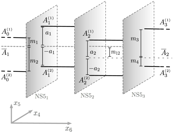
Figure 1: NS5 and D4 brane set up for the conformal SU(2)$\,\times\,$SU(2) quiver theory.

The brane configuration is best described in terms of the complex combinations

$$x^{4}+\mathrm{i}\,x^{5}\,\equiv\,2\pi\alpha^{\prime}v\qquad\mbox{and}\qquad x^{6}+\mathrm{i}\,x^{10}\,\equiv\,s~{},$$ (2.2)

or their exponentials

$$w\,\equiv\,\mathrm{e}^{\frac{2\pi\alpha^{\prime}v}{R_{5}}}=\,\mathrm{e}^{\beta v}\qquad\mbox{and}\qquad t\,\equiv\,\mathrm{e}^{\frac{s}{R_{10}}}$$ (2.3)

which are single-valued under integer shifts of $x^{5}$ and $x^{10}$ along the respective circumferences. Notice that we have introduced factors of $\alpha^{\prime}$ to assign to $v$ scaling dimensions of a mass; this choice will be particularly convenient for our later purposes. For each NS5_i the variable $s_{i}$ satisfies the Poisson equation in the $v$-plane [44]

$$\nabla^{2}\,s_{i}=f_{i}$$ (2.4)

where the source term in the right hand side describes the pulling on the $i$-th NS5 brane due to the D4 branes terminating on it from each side. For our configuration this is simply a sum of four $\delta$-functions localized at the relevant D4 positions in the $v$-plane. We denote the positions of the flavour D4 branes on the left by $\big{(}A^{(1)}_{0},A^{(2)}_{0}\big{)}$, those of the flavour D4 branes on the right by $\big{(}A^{(1)}_{n+1},A^{(2)}_{n+1}\big{)}$, and those of the colour D4 branes between NS5_i and NS5_i+1 by $\big{(}A^{(1)}_{i},A^{(2)}_{i}\big{)}$. Since $x^{5}$ is compact, we have to take into account also the infinite images of these brane positions and hence the solution of the Poisson equation (2.4) is

$$\frac{s_{i}}{R_{10}} =\sum_{k=-\infty}^{\infty}\!\Bigg{\{}\!\log\Big{[}\beta\big{(}v-A^{(1)}_{i-1}\big{)}-2\pi\mathrm{i}k\Big{]}+\log\Big{[}\beta\big{(}v-A^{(2)}_{i-1}\big{)}-2\pi\mathrm{i}k\Big{]}$$ (2.5)

$$\quad\quad-\log\Big{[}\beta\big{(}v-A^{(1)}_{i}\big{)}-2\pi\mathrm{i}k\Big{]}-\log\Big{[}\beta\big{(}v-A^{(2)}_{i}\big{)}-2\pi\mathrm{i}k\Big{]}\Bigg{\}}+\mbox{const.}$$

for $i=1,\ldots,n+1$. Using the identity

$$\prod_{k=1}^{\infty}\left(1+\frac{x^{2}}{k^{2}}\right)=\frac{\sinh\pi x}{\pi x}~{},$$ (2.6)

and exponentiating the above result, this can be rewritten as

$$\mathrm{e}^{\frac{s_{i}}{R_{10}}}=\,t_{i}~{}\frac{\sinh\left(\frac{\beta}{2}\big{(}v-A^{(1)}_{i-1}\big{)}\right)\sinh\left(\frac{\beta}{2}\big{(}v-A^{(2)}_{i-1}\big{)}\right)}{\sinh\left(\frac{\beta}{2}\big{(}v-A^{(1)}_{i}\big{)}\right)\sinh\left(\frac{\beta}{2}\big{(}v-A^{(2)}_{i}\big{)}\right)}~{},$$ (2.7)

where $t_{i}$ is related to the integration constant in (2.5). The asymptotic positions of the NS5 branes can be obtained by taking the limits $\mbox{Re}\,v\rightarrow-\infty$ (i.e. $w\rightarrow 0$) and $\mbox{Re}\,v\rightarrow+\infty$ (i.e. $w\rightarrow\infty$) and are given by

$$\mathrm{e}^{\frac{s_{i}}{R_{10}}}\,\Big{|}_{w\to 0}=t_{i}\,\sqrt{\frac{\widetilde{A}^{(1)}_{i-1}\,\widetilde{A}^{(2)}_{i-1}}{\widetilde{A}^{(1)}_{i}\widetilde{A}^{(2)}_{i}}}\,\equiv\,t^{(0)}_{i}~{},\qquad\mathrm{e}^{\frac{s_{i}}{R_{10}}}\,\Big{|}_{w\to\infty}=t_{i}\,\sqrt{\frac{\widetilde{A}^{(1)}_{i}\widetilde{A}^{(2)}_{i}}{\widetilde{A}^{(1)}_{i-1}\widetilde{A}^{(2)}_{i-1}}}\,\equiv\,t^{(\infty)}_{i}~{}.$$ (2.8)

Here we have introduced tilded variables according to

$$\widetilde{A}=\mathrm{e}^{\beta\,A}$$ (2.9)

for any given $A$.

As argued in [44], the difference in the asymptotic positions of the NS5 branes is related to the complexified UV coupling constant of the gauge theory on the color D-branes; more precisely if we define

$$\tau_{i}=\frac{\theta_{i}}{\pi}+\mathrm{i}\,\frac{8\pi}{g_{i}^{2}}$$ (2.10)

where $\theta_{i}$ and $g_{i}$ are the $\theta$-angle and the Yang-Mills coupling for the SU(2) theory of the $i$-th node, we have

$$\pi\mathrm{i}\tau_{i}\,\sim\,\frac{s_{i}-s_{i+1}}{R_{10}}~{}.$$ (2.11)

However, since the distance between the NS5 branes is different in the two asymptotic regions $\mbox{Re}\,v\rightarrow\pm\infty$, there is some ambiguity in this definition. We fix it as in [44, 45] and use

$$q_{i}=\mathrm{e}^{\pi\mathrm{i}\tau_{i}}=\frac{t_{i}}{t_{i+1}}\quad\text{or, equivalently,}\quad t_{i}=t_{n+1}\,\prod_{j=i}^{n}q_{j}~{}.$$ (2.12)

The overall constant $t_{n+1}$ drops out from all equations and can be set to 1 without any loss of generality. In subsequent sections we will confirm that the above identification of the UV coupling constants is fully consistent with the Nekrasov multi-instanton calculations.

2.2 The 5-dimensional curve

The general SW curve for the 5-dimensional theory defined on the color D4 branes takes the form of a polynomial equation [44] in the $t$ and $w$ variables introduced in (2.3):

$$\sum_{p,q}C_{p,q}\,t^{p}w^{q}=0~{}.$$ (2.13)

Since there are always only two D4 branes in each region and in total we have $(n+1)$ NS5 branes, the polynomial in (2.13) must be of degree 2 in $w$ and of degree $(n+1)$ in $t$. Of course, there are two equivalent ways of writing it. One is:

$$\mathcal{C}_{1}:\quad w^{2}\,Q_{2}(t)+w\,Q_{1}(t)+Q_{0}(t)=0~{},$$ (2.14)

where the $Q$’s are polynomials in $t$ of degree $(n+1)$; the other is:

$$\mathcal{C}_{2}:\quad t^{n+1}\,P_{n+1}(w)+t^{n}\,P_{n}(w)+\cdots t\,P_{1}(w)+P_{0}(w)=0~{},$$ (2.15)

where each of the $P$’s is a polynomial of degree $2$ in $w$. Using the known solutions of $t$ when $w\to 0$ or $w\to\infty$, the form $\mathcal{C}_{1}$ can be written as

$$\mathcal{C}_{1}:\quad w^{2}\,\prod_{i=1}^{n+1}\big{(}t-t^{(\infty)}_{i}\big{)}+w\,Q_{2}(t)+d^{\prime}\,\prod_{i=1}^{n+1}\big{(}t-t^{(0)}_{i}\big{)}=0~{}.$$ (2.16)

Having fixed to 1 the coefficient of the highest term $w^{2}t^{n+1}$, in (2.16) there are $(n+3)$ undetermined constants in this equation: $d^{\prime}$ and the $(n+2)$ coefficients of $Q_{2}$. On the other hand, using the fact that when $t\to 0$ and $t\to\infty$ there are two flavour branes at $w=(\widetilde{A}^{(1)}_{0},\widetilde{A}^{(2)}_{0})$ and $w=(\widetilde{A}^{(1)}_{n+1},\widetilde{A}^{(2)}_{n+1})$ respectively, we can write the form $\mathcal{C}_{2}$ of the curve as

$$\mathcal{C}_{2}:\quad t^{n+1}\,\prod_{\alpha=1}^{2}\big{(}w-\widetilde{A}^{(\alpha)}_{n+1}\big{)}+t^{n}\,P_{n}(w)+\cdots t\,P_{1}(w)+d\,\prod_{\alpha=1}^{2}\big{(}w-\widetilde{A}^{(\alpha)}_{0}\big{)}=0~{}.$$ (2.17)

Again we have fixed to 1 the coefficient of the highest term $w^{2}\,t^{n+1}$, but in this form there are $(3n+1)$ undetermined parameters: $d$ and the three coefficients for each of the $n$ polynomials $P_{k}$’s.

Equating the two forms (2.16) and (2.17) allows us to find relations that determine some of the curve parameters: for instance, by comparing the coefficients of $w^{2}\,t^{0}$ and $w^{0}\,t^{n+1}$ in the two expressions we get

$$d=(-1)^{n+1}\prod_{i=1}^{n+1}t^{(\infty)}_{i}~{},\qquad d^{\prime}=\widetilde{A}^{(1)}_{n+1}\widetilde{A}^{(2)}_{n+1}~{}.$$ (2.18)

Similarly, by comparing the coefficients of $w\,t^{0}$ and $w\,t^{n+1}$ we find that the undetermined polynomial $Q_{2}(t)$ in (2.16) takes the form

$$Q_{2}(t)=-\big{(}\widetilde{A}^{(1)}_{n+1}+\widetilde{A}^{(2)}_{n+1}\big{)}\,t^{n+1}+\sum_{k=1}^{n}c_{k}\,t^{k}+(-1)^{n}\big{(}\widetilde{A}^{(1)}_{0}+\widetilde{A}^{(2)}_{0}\big{)}\prod_{i=1}^{n+1}t^{(\infty)}_{i}~{}.$$ (2.19)

Proceeding in a similar way one can fix the coefficients of $w^{2}$ and $w^{0}$ in the $n$ quadratic polynomials $P_{i}$’s of (2.17). In the end, all but $n$ parameters in the SW curve are fixed; the $n$ free coefficients that remain parametrize the Coulomb branch of the $\mathrm{SU}(2)^{n}$ quiver gauge theory. One subtlety is that the constant terms in (2.16) and (2.17) match only if the following identity is satisfied:

$$\widetilde{A}^{(1)}_{0}\,\widetilde{A}^{(2)}_{0}\,\prod_{i=1}^{n+1}t^{(\infty)}_{i}=\widetilde{A}^{(1)}_{n+1}\,\widetilde{A}^{(2)}_{n+1}\,\prod_{i=1}^{n+1}t^{(0)}_{i}~{}.$$ (2.20)

Using the explicit expressions (2.8) for the asymptotic positions of the NS5 branes, we can check that this is identically satisfied and both sides are equal to $(\widetilde{A}^{(1)}_{0}\,\widetilde{A}^{(2)}_{0}\widetilde{A}^{(1)}_{n+1}\,\widetilde{A}^{(2)}_{n+1})^{1/2}$. This shows that indeed the two forms $\mathcal{C}_{1}$ and $\mathcal{C}_{2}$ of the SW curve are fully equivalent.

2.3 The 4-dimensional curve

We now dimensionally reduce to four dimensions by first performing a T-duality and then taking the limit $\beta\rightarrow 0$. To find explicit expressions it necessary to introduce the physical parameters of the 4-dimensional theory and rewrite the geometric positions of the various branes in terms of these. In order to do this, for each pair of colour D4 branes we define the center of mass and relative positions in the $v$-plane according to

$$A^{(1)}_{i}=a_{i}+\bar{A}_{i}~{},\qquad A^{(2)}_{i}=-a_{i}+\bar{A}_{i}$$ (2.21)

for $i=1,\ldots,n$. The relative position $a_{i}$ is identified with the vacuum expectation value of the adjoint scalar field $\Phi_{i}$ of the $i$-th SU(2) factor in the quiver theory. Furthermore we remove the global U(1) factor by requiring

$$\bar{A}_{1}+\cdots+\bar{A}_{n}=0~{},$$ (2.22)

and identify the relative positions of the centers of mass with the physical masses of the bi-fundamental hypermultiplets, i.e.

$$m_{i,i+1}=\bar{A}_{i}-\bar{A}_{i+1}$$ (2.23)

for $i=1,\ldots,n-1$. Finally, the physical masses of the fundamental hypermultiplets attached to the first and the last NS5 branes are related to the positions of the flavour D4 branes measured with respect to the first and last center of mass in the $v$-plane, namely

$$m_{1}=A^{(1)}_{0}-\bar{A}_{1}~{},~{}~{}~{}m_{2}=A^{(2)}_{0}-\bar{A}_{1}~{},~{}~{}~{}m_{3}=A^{(1)}_{n+1}-\bar{A}_{n}~{},~{}~{}~{}m_{4}=A^{(2)}_{n+1}-\bar{A}_{n}~{}.$$ (2.24)

All this is displayed in Fig. 1 for the case $n=2$.

Given this set-up, it is rather straightforward to obtain the 4-dimensional SW curve. However, in general it is not so simple to write explicit expressions in terms of the relevant physical parameters. Thus, we discuss in detail the following three cases:

• the conformal $\mathrm{SU}(2)^{n}$ quiver with massless hypermultiplets;

• the SU(2) theory with $N_{f}=4$ massive fundamental flavours;

• the SU(2)$\,\times\,$SU(2) quiver theory with generically massive hypermultiplets.

$\bullet$ The conformal $\mathrm{SU}(2)^{n}$ quiver

When all matter hypermultiplets are massless the curve equation drastically simplifies. Indeed, all stacks of colour branes have the same center of mass positions, so that (2.22) implies that $\bar{A}_{i}=0$ for $i=1,\ldots,n$. Moreover, setting to zero the four fundamental masses implies that $A^{(1)}_{0}=A^{(2)}_{0}=A^{(1)}_{n+1}=A^{(2)}_{n+1}=0$. Using this, we have

$$t^{(0)}_{i}=t^{(\infty)}_{i}=t_{i}$$ (2.25)

where the constants $t_{i}$ are defined in terms of the gauge couplings $q_{i}$ according to (2.12). The 5-dimensional curve (2.16) then becomes

$$w^{2}\,\prod_{i=1}^{n+1}(t-t_{i})-2\,w\Big{(}t^{n+1}-\frac{1}{2}\sum_{k=1}^{n}c_{k}\,t^{k}-(-1)^{n}\prod_{i=1}^{n+1}t_{i}\Big{)}+\prod_{i=1}^{n+1}(t-t_{i})=0~{}.$$ (2.26)

We now take the 4-dimensional limit $\beta\to 0$ after writing $c_{k}=c_{k0}+c_{k1}\beta+c_{k2}\beta^{2}+\cdots$ and $w=\mathrm{e}^{\beta v}$. The $\mathcal{O}(\beta^{0})$ and $\mathcal{O}(\beta^{1})$ terms yield algebraic constraints for $c_{k0}$ and $c_{k1}$ that can be easily solved. Instead, the $\mathcal{O}(\beta^{2})$ term leads to the 4-dimensional SW curve. Writing $v=x\,t$ and setting $t_{n+1}=1$, the curve becomes

$$x^{2}(t)=\frac{\mathcal{P}_{n-1}(t)}{t\,(t-t_{1})\cdots(t-t_{n})(t-1)}$$ (2.27)

where $\mathcal{P}_{n-1}(t)$ is a polynomial of degree $n-1$, whose $n$ coefficients parametrize the Coulomb branch of the $\mathrm{SU}(2)^{n}$ theory. This is precisely the form of the SW curve discussed in [1].

When the matter multiplets are massive, things become more involved. While it is always quite straightforward to write formal expressions, it is not always immediate to identify the meaning of the various coefficients in terms of the physical parameters of the gauge theory. Thus to avoid clumsy general expressions we discuss in detail the cases with $n=1$ and $n=2$.

$\bullet$ The SU(2) theory with $N_{f}=4$

When $n=1$ the formulæ (2.21)-(2.24) lead to

$$A_{0}^{(1)}=m_{1}~{},\quad A_{0}^{(2)}=m_{2}~{},\quad A_{1}^{(1)}=a~{},\quad A_{1}^{(2)}=-a~{},\quad A_{2}^{(1)}=m_{3}~{},\quad A_{2}^{(2)}=m_{4}~{},\quad$$ (2.28)

where $a$ is the vacuum expectation of the adjoint scalar field $\Phi$. Then the curve (2.16) becomes

$$w^{2}\big{(}t-t_{1}^{(\infty)}\big{)}\!\big{(}t-t_{2}^{(\infty)}\big{)}-w\Big{[}\big{(}\widetilde{m}_{3}+\widetilde{m}_{4}\big{)}t^{2}-c\,t+\big{(}\widetilde{m}_{1}+\widetilde{m}_{2}\big{)}t_{1}^{(\infty)}t_{2}^{(\infty)}\Big{]}+\widetilde{m}_{3}\widetilde{m}_{4}\big{(}t-t_{1}^{(0)}\big{)}\!\big{(}t-t_{2}^{(0)}\big{)}=0$$ (2.29)

where, according to (2.8) and (2.12),

$$t_{1}^{(0)}=q\,\sqrt{\widetilde{m}_{1}\widetilde{m}_{2}}~{},\quad t_{1}^{(\infty)}=\frac{q}{\sqrt{\widetilde{m}_{1}\widetilde{m}_{2}}}~{},\quad t_{2}^{(0)}=\frac{1}{\sqrt{\widetilde{m}_{3}\widetilde{m}_{4}}}~{},\quad t_{2}^{(\infty)}=\sqrt{\widetilde{m}_{3}\widetilde{m}_{4}}$$ (2.30)

and we are using the tilded variables $\widetilde{m}_{i}$ according to the notation introduced in Eq. (2.9). To obtain the 4-dimensional curve we expand $w$, $c$ and all tilded variables in powers of $\beta$. The $\mathcal{O}(\beta^{0})$ and $\mathcal{O}(\beta^{1})$ terms can be set to zero by suitably choosing the first two coefficients in the expansion of $c$, while the $\mathcal{O}(\beta^{2})$ term yields the SW curve for the SU(2) $N_{f}=4$ theory. The result is [62, 63, 45]

$$v^{2}(t-q)(t-1)-v\Big{[}(m_{3}+m_{4})t^{2}-q\sum_{f=1}^{4}m_{f}\,t+q(m_{1}+m_{2})\Big{]}+m_{3}m_{4}\,t^{2}+u\,t+q\,m_{1}m_{2}=0~{}.$$ (2.31)

Here we have absorbed all terms linear in $t$ and independent of $v$ by redefining $c$ into a new parameter $u$. A simple dimensional analysis reveals that $u$ has dimensions of $(\mathrm{mass})^{2}$. As pointed out in [1] it is a bit arbitrary to define the origin for this $u$ parameter when masses are present. Here we fix such arbitrariness by requiring

$$u\,\big{|}_{q\to 0}=\,a^{2}~{}.$$ (2.32)

Shifting away the linear term in $v$ in (2.31) and writing $v=x\,t$, we get [62, 63, 45]

$$x^{2}(t)=\frac{\mathcal{P}_{4}(t)}{t^{2}(t-q)^{2}(t-1)^{2}}$$ (2.33)

where $\mathcal{P}_{4}(t)$ is a fourth-order polynomial in $t$ of the form

$$\mathcal{P}_{4}(t)=-u\,t\,(t-q)(t-1)+\mathcal{M}_{4}(t)$$ (2.34)

where we have collected in $\mathcal{M}_{4}(t)$ all terms that depend on the masses. The explicit expression of this polynomial is given in (B.1). Using it and choosing a specific determination for the square-root, one easily finds

$$\mathrm{Res}_{\,t=0}\left(x(t)\right) =\frac{m_{1}-m_{2}}{2}~{},\qquad\mathrm{Res}_{\,t=q}\left(x(t)\right)=\frac{m_{1}+m_{2}}{2}~{},$$ (2.35)

$$\mathrm{Res}_{\,t=1}\left(x(t)\right) =\frac{m_{3}+m_{4}}{2}~{},\qquad\mathrm{Res}_{\,t=\infty}\left(x(t)\right)=\frac{m_{4}-m_{3}}{2}~{}.$$

$\bullet$ The SU(2)$\,\times\,$SU(2) quiver theory

For a 2-node quiver (see Fig. 1), the formulæ (2.21)-(2.24) read

$$A_{1}^{(0)} =m_{1}+\frac{m_{12}}{2}~{},~{}\,A_{2}^{(0)}=m_{2}+\frac{m_{12}}{2}~{},~{}\,A_{1}^{(1)}=a_{1}+\frac{m_{12}}{2}~{},~{}\,A_{2}^{(1)}=-a_{1}+\frac{m_{12}}{2}~{},$$ (2.36)

$$A_{1}^{(2)} =a_{2}-\frac{m_{12}}{2}~{},~{}\,A_{2}^{(2)}=-a_{2}-\frac{m_{12}}{2}~{},~{}\,A_{1}^{(3)}=m_{3}-\frac{m_{12}}{2}~{},~{}\,A_{2}^{(3)}=m_{4}-\frac{m_{12}}{2}$$

where $a_{1}$ and $a_{2}$ are the vacuum expectation values of the adjoint scalars $\Phi_{1}$ and $\Phi_{2}$ of the two SU(2) factors. With this configuration the 5-dimensional curve (2.16) becomes

$$w^{2}\prod_{i=1}^{3}\big{(}t-t^{(\infty)}_{i}\big{)} -w\,\Big{(}\frac{\widetilde{m}_{3}+\widetilde{m}_{4}}{\sqrt{\widetilde{m}_{12}}}\,t^{3}-c_{2}\,t^{2}-c_{1}\,t$$ (2.37)

$$~{}~{}-\sqrt{\widetilde{m}_{12}}\big{(}\widetilde{m}_{1}+\widetilde{m}_{2}\big{)}\prod_{i=1}^{3}t^{(\infty)}_{i}\Big{)}+\frac{\widetilde{m}_{3}\widetilde{m}_{4}}{\widetilde{m}_{12}}\,\prod_{i=1}^{3}\big{(}t-t^{(0)}_{i}\big{)}=0$$

where the asymptotic values are

$$t_{1}^{(0)} =t_{1}\sqrt{\widetilde{m}_{1}\widetilde{m}_{2}}~{},\quad~{}t_{2}^{(0)}=t_{2}\,\widetilde{m}_{12}~{},\quad~{}t_{3}^{(0)}=\frac{1}{\sqrt{\widetilde{m}_{3}\widetilde{m}_{4}}}~{},$$ (2.38)

$$t_{1}^{(\infty)} =\frac{t_{1}}{\sqrt{\widetilde{m}_{1}\widetilde{m}_{2}}}~{},\qquad~{}t_{2}^{(\infty)}=\frac{t_{2}}{\widetilde{m}_{12}}~{},\quad~{}t_{3}^{(\infty)}=\sqrt{\widetilde{m}_{3}\widetilde{m}_{4}}$$

with

$$t_{1}=q_{1}q_{2}~{},\qquad t_{2}=q_{2}~{}.$$ (2.39)

We now take the 4-dimensional limit $\beta\to 0$, proceeding as in the previous examples. The resulting SW curve is

$$v^{2}(t-t_{1})(t-t_{2})(t-1)$$

$$-v\,\Bigg{[}(m_{3}+m_{4}-m_{12})\,t^{3}-\bigg{(}\Big{(}\sum_{f=1}^{4}m_{f}-m_{12}\Big{)}\,t_{1}+(m_{3}+m_{4}+m_{12})\,t_{2}-m_{12}\bigg{)}t^{2}$$

$$~{}+\bigg{(}(m_{1}+m_{2}-m_{12})\,t_{1}+m_{12}\,t_{2}+\Big{(}\sum_{f=1}^{4}m_{f}+m_{12}\Big{)}\,t_{1}\,t_{2}\bigg{)}\,t-(m_{1}+m_{2}+m_{12})\,t_{1}\,t_{2}\Bigg{]}$$

$$+\Bigg{[}\Big{(}m_{3}-\frac{m_{12}}{2}\Big{)}\Big{(}m_{4}-\frac{m_{12}}{2}\Big{)}\,t^{3}-\Big{(}\frac{m_{12}^{2}}{4}-u_{2}\Big{)}\,t^{2}+\Big{(}\frac{m_{12}^{2}}{4}-u_{1}\Big{)}t_{2}\,t$$

$$~{}-\Big{(}m_{1}+\frac{m_{12}}{2}\Big{)}\Big{(}m_{2}+\frac{m_{12}}{2}\Big{)}\,t_{1}\,t_{2}\Bigg{]}=0~{}.$$ (2.40)

Here we have exploited the freedom to redefine the arbitrary coefficients $c_{1}$ and $c_{2}$ into the parameters $u_{1}$ and $u_{2}$ for which we require the following classical limit

$$u_{1}\,\big{|}_{q_{1},q_{2}\to 0}=\,a_{1}^{2}\quad\quad\mbox{and}\qquad u_{2}\,\big{|}_{q_{1},q_{2}\to 0}=\,a_{2}^{2}~{}.$$ (2.41)

In Section 4 we will confirm the validity of this requirement.

In order to put the curve in a more convenient form, we shift away the linear term in $v$ in (2.40) and then write $v=x\,t$, obtaining

$$x^{2}(t)=\frac{\mathcal{P}_{6}(t)}{t^{2}\,(t-t_{1})^{2}(t-t_{2})^{2}(t-1)^{2}}~{},$$ (2.42)

where $\mathcal{P}_{6}(t)$ is a polynomial of degree six in $t$ of the form

$$\mathcal{P}_{6}(t)=-t\,(u_{2}\,t-t_{2}\,u_{1})(t-t_{1})(t-t_{2})(t-1)+\mathcal{M}_{6}(t)$$ (2.43)

with $\mathcal{M}_{6}(t)$ containing all mass-dependent terms. The explicit expression of this polynomial is given in (B.3). Using it we find

$$\mathrm{Res}_{\,t=0}\left(x(t)\right) = \frac{m_{1}-m_{2}}{2}~{},\quad\mathrm{Res}_{\,t=t_{1}}\left(x(t)\right)=\frac{m_{1}+m_{2}}{2}~{},\quad\mathrm{Res}_{\,t=t_{2}}\left(x(t)\right)=m_{12}~{},$$ (2.44)

$$\!\!\!\!\!\!\!\!\!\!\!\mathrm{Res}_{\,t=1}\left(x(t)\right)=\frac{m_{3}+m_{4}}{2}~{},\quad\mathrm{Res}_{\,t=\infty}\left(x(t)\right)=\frac{m_{4}-m_{3}}{2}~{}.$$

2.4 From the 4-dimensional curve to the prepotential

The spectral curve (2.42) encodes all relevant information about the effective quiver gauge theory through the SW differential

$$\lambda=x(t)dt~{}.$$ (2.45)

If we differentiate $\lambda$ with respect to $u_{1}$ and $u_{2}$, we get (up to normalizations which are irrelevant for our present purposes)

$$\frac{\partial\lambda}{\partial u_{1}}\simeq\frac{dt}{y}~{},\qquad\frac{\partial\lambda}{\partial u_{2}}\simeq\frac{t\,dt}{y}~{},$$ (2.46)

where

$$y^{2}=\mathcal{P}_{6}(t)~{}.$$ (2.47)

This is the standard equation defining a genus-2 Riemann surface. Such a surface admits a canonical symplectic basis with two pairs of 1-cycles $(\alpha_{1},\alpha_{2})$ and $(\beta_{1},\beta_{2})$ whose intersection matrix is $\alpha_{i}\cap\alpha_{j}=\beta_{i}\cap\beta_{j}=\delta_{ij}$. The periods of the SW differential $\lambda$ along these cycles represent the quantities $a_{i}$ and $a_{i}^{D}$ in the effective gauge theory, namely

$$a_{i}=\frac{1}{2\pi\mathrm{i}}\oint_{\alpha_{i}}\lambda~{},\qquad a_{i}^{D}=\frac{1}{2\pi\mathrm{i}}\oint_{\beta_{i}}\lambda~{}.$$ (2.48)

Through these relations, $a_{i}$ and $a_{i}^{D}$ are determined as functions of the $u_{i}$’s (and, of course, of the UV couplings $q_{i}$ and of the mass parameters). Inverting these relations, one can express the $u_{i}$’s in terms of the $a_{i}$’s and, substituting them into the dual periods, obtain $a_{i}^{D}(a)$. Since

$$a_{i}^{D}(a)=\frac{\partial F}{\partial a_{i}}~{},$$ (2.49)

one can reconstruct in this way the prepotential $F$ (up to $a$-independent terms). By comparing this prepotential with the one obtained from the multi-instanton calculus via localization one can therefore test the validity of the proposed form of the SW curve.

However, an alternative and more efficient approach has been presented in [47, 48] in which the difficult computations of the dual periods $a_{i}^{D}$ are avoided and the effective prepotential is directly put in relation with the residues of the quadratic differential $x^{2}(t)dt^{2}$ in the following way

$$\mathrm{Res}_{\,t=t_{i}}\left(x^{2}(t)\right)=\frac{\partial{\widetilde{F}}}{\partial t_{i}}~{}.$$ (2.50)

As we will show in more detail below, assuming this relation and just computing the $\alpha$-periods of the SW differential we can readily reconstruct $\widetilde{F}$ from the spectral curve and check that it coincides with the effective prepotential $F$ computed via localization up to mass-dependent but $a$-independent shifts (so that $\widetilde{F}$ and $F$ encode the same effective gauge couplings); the expression of these shifts is however rather interesting, and we will comment on this in the next sections.

3 The SU(2) theory with $N_{f}=4$

We show how to derive the effective prepotential for the SU(2) $N_{f}=4$ theory starting from the curve (2.33) and the residue formula (2.50) which in this case reads

$$\mathrm{Res}_{\,t=q}\left(x^{2}(t)\right)=\frac{\partial\widetilde{F}}{\partial q}~{}.$$ (3.1)

In doing this we do not only provide a generalization of the results presented in [48], but also set the stage for the discussion of the quiver theory in the next section.

Using the curve (2.33) and the explicit expression of the polynomial $\mathcal{P}_{4}$ reported in (B.1), the above residue formula leads to

$$q(1-q)\frac{\partial\widetilde{F}}{\partial q}=u-\frac{1-q}{2}\left(m_{1}^{2}+m_{2}^{2}\right)+\frac{q}{2}\left(m_{1}+m_{2}\right)\left(m_{3}+m_{4}\right)+q\left(m_{1}m_{2}+m_{3}m_{4}\right)~{}.$$ (3.2)

Combining this with the residues (2.35) amounts to rewrite the SW curve (2.33) as

$$x^{2}(t)= \,\frac{(m_{1}-m_{2})^{2}}{4t^{2}}+\frac{(m_{1}+m_{2})^{2}}{4(t-q)^{2}}+\frac{(m_{3}+m_{4})^{2}}{4(t-1)^{2}}-\frac{m_{1}^{2}+m_{2}^{2}+2m_{3}m_{4}}{2t(t-1)}$$ (3.3)

$$+\frac{q(q-1)}{t(t-q)(t-1)}\,\frac{\partial\widetilde{F}}{\partial q}~{}.$$

We now clarify the meaning of $\widetilde{F}$. Imposing in (3.2) the boundary value (2.32) for $u$, we easily find

$$q\frac{\partial\widetilde{F}}{\partial q}\,\Big{|}_{q\to 0}=\,a^{2}-\frac{1}{2}\left(m_{1}^{2}+m_{2}^{2}\right)~{},$$ (3.4)

from which we deduce that $\widetilde{F}$ cannot be directly identified with the effective gauge theory prepotential, whose classical term is in fact $F_{\mathrm{cl}}=a^{2}\log q$. Therefore, to ensure the proper classical limit we shift $\widetilde{F}$ according to

$$\widetilde{F}=\widehat{F}-\frac{1}{2}\left(m_{1}^{2}+m_{2}^{2}\right)\log q~{},$$ (3.5)

and rewrite (3.2) as

$$q(1-q)\frac{\partial\widehat{F}}{\partial q}=u+\frac{q}{2}\left(m_{1}+m_{2}\right)\left(m_{3}+m_{4}\right)+q\left(m_{1}m_{2}+m_{3}m_{4}\right)~{}.$$ (3.6)

The function $\widehat{F}$ has the correct classical limit, but it is not yet the gauge theory prepotential since it is determined by an equation in which the four masses do not appear on equal footing. There are two independent ways to remedy this and restore complete symmetry among the flavors, namely by redefining $\widehat{F}$ as

$$\mathrm{I)} : \quad\widehat{F}=F_{\mathrm{I}}+\frac{1}{2}\log(1-q)\left(m_{1}+m_{2}\right)\left(m_{3}+m_{4}\right)~{},$$ (3.7)

$$\mathrm{II)} : \quad\widehat{F}=F_{\mathrm{II}}-\frac{1}{2}\log(1-q)\left(m_{1}m_{2}+m_{3}m_{4}\right)~{}.$$ (3.8)

In this way, from (3.6) we get

$$\mathrm{I)} : \quad q(1-q)\frac{\partial{F_{\mathrm{I}}}}{\partial q}\equiv(1-q)\,U_{\mathrm{I}}=u+q\sum_{f<f^{\prime}}m_{f}m_{f}^{\prime}~{},$$ (3.9)

$$\mathrm{II)} : \quad q(1-q)\frac{\partial{F_{\mathrm{II}}}}{\partial q}\equiv(1-q)\,U_{\mathrm{II}}=u+\frac{q}{2}\sum_{f<f^{\prime}}m_{f}m_{f}^{\prime}~{}.$$ (3.10)

The minor difference in the numerical coefficient in front of the mass terms in these two equations is, actually, quite significant. In fact, as we will see, $F_{\mathrm{I}}$ is the Nekrasov prepotential for the SU(2) $N_{f}=4$ theory, while $F_{\mathrm{II}}$ is the SO(8) invariant prepotential that can be derived from the SW curve of [3] expressed in terms of the UV coupling $q$.

To verify this statement in an explicit way, we take

$$m_{1}=m_{2}=m~{},\quad m_{3}=m_{4}=M~{}.$$ (3.11)

This is a simple choice of masses that allows us to exhibit all non-trivial features of the calculation. With these masses the curve (2.33) becomes

$$x^{2}(t)=\frac{\mathcal{P}_{2}(t)}{t(t-1)^{2}(t-q)^{2}}$$ (3.12)

where

$$\mathcal{P}_{2}(t)\!\! = \!\!-Ct^{2}+\Big{(}u(1+q)-q(m-M)^{2}+q^{2}(m+M)^{2}\Big{)}t-q\Big{(}u-\left(1-q\right)m^{2}+2qmM\Big{)}$$ (3.13)

$$= C(e_{2}-t)(t-e_{3})\phantom{\Big{|}}$$

with

$$C=u+2qmM-M^{2}(1-q)~{}.$$ (3.14)

The expressions of the two roots $e_{2}$ and $e_{3}$ can be easily obtained by solving the quadratic equation $\mathcal{P}_{2}(t)=0$; in the 1-instanton approximation we find

$$e_{2} =q\Big{(}1-\frac{m^{2}}{u}+q\frac{m^{2}\left(u^{2}+M^{2}u+2mMu-m^{2}M^{2}\right)}{u^{3}}+\ldots\Big{)}~{},$$ (3.15)

$$e_{3} =1+\frac{M^{2}}{u-M^{2}}+q\frac{M^{2}\left(m^{2}M^{2}-m^{2}u-2mMu-u^{2}\right)}{u(u-M^{2})}+\ldots$$

The SW differential associated to the spectral curve (3.12) is

$$\lambda=x(t)dt=\sqrt{\frac{(e_{2}-t)(t-e_{3})}{t}}\,\frac{\sqrt{C}\,dt}{(1-t)(t-q)}~{};$$ (3.16)

it possess four branch points at $t=0,\,e_{2},\,e_{3}$ and $\infty$ and two simple poles at $t=q$ and $1$. This singularity structure is shown in Fig. 2. The cross-ratio of the four branch points is

$$\zeta = \frac{e_{2}}{e_{3}}=q\left(1-\frac{(m^{2}+M^{2})u-m^{2}M^{2}}{u^{2}}\right)$$

$$~{}+q^{2}\left(\frac{(m^{2}+M^{2})u^{3}+2mM(m^{2}+M^{2})u^{2}-2m^{2}M^{2}(m+M)^{2}u+2m^{4}M^{4}}{u^{4}}\right)+\ldots$$

In the massless limit, note that the cross ratio reduces to the Nekrasov counting parameter $q$, as expected. As always, we identify the $\alpha$-period of the SW differential with the vacuum expectation value $a$, namely

$$a=\frac{1}{2\pi\mathrm{i}}\oint_{\alpha}\lambda=~{}\mathrm{Res}_{\,t=q}\left(\lambda\right)+\frac{\sqrt{C}}{\pi}\int_{0}^{e_{2}}\sqrt{\frac{e_{2}-t}{t}}\,\frac{\sqrt{e_{3}-t}}{(1-t)(q-t)}\,dt~{}.$$ (3.18)

Figure 2: Branch-cuts and singularities of the $\alpha$-period of SW differential $\lambda$ of the SU(2) $N_{f}=4$ theory.

It is important to stress that the $\alpha$-cycle corresponds to a closed contour encircling both the branch cut from $0$ to $e_{2}$ and the simple pole of $\lambda$ at $t=q$, see Fig. 2. With this prescription, the $\alpha$-cycle has a smooth limit when the masses are set to zero. This explains the two terms on the right hand side of (3.18): the residue over the pole in $t=q$, which in view of (2.35) is simply $m$, and the integral over the branch cut. This integral is explicitly evaluated in Appendix C (see in particular (C.9)); in the final result the mass term coming from the residue is canceled and we are left with

$$a =\frac{\sqrt{C(e_{3}-q)}}{1-q}+\frac{\sqrt{C}}{1-q}\sum_{n,\ell=0}^{\infty}(-1)^{\ell}\binom{1/2}{n+1}\binom{1/2}{n+\ell+1}\frac{e_{2}^{n+1}\,q^{\ell}}{e_{3}^{n+\ell+1/2}}$$ (3.19)

$$~{}~{}~{}~{}-\frac{\sqrt{C}}{1-q}\sum_{n=0}^{\infty}\sum_{\ell=0}^{n}(-1)^{(n+\ell)}\binom{1/2}{n+1}\binom{1/2}{\ell}\frac{e_{2}^{n+1}}{e_{3}^{\ell-1/2}}~{}.$$

Exploiting the expressions of the roots $e_{2}$ and $e_{3}$, it is not difficult to realize that the right hand side of (3.19) has an expansion in positive powers of $q$ and that only a finite number of terms contribute to a given order, i.e. to a given instanton number. For example, using (3.14) and (3.15), up to one instanton we find

$$a=\sqrt{u}\left(1+q\,\frac{u^{2}+m^{2}u+4mMu+M^{2}u-m^{2}M^{2}}{4u^{2}}+\ldots\right)~{},$$ (3.20)

which can be inverted leading to

$$u=a^{2}\left(1-q\,\frac{a^{4}+m^{2}a^{2}+4mMa^{2}+M^{2}a^{2}-m^{2}M^{2}}{2a^{2}}+\ldots\right)~{}.$$ (3.21)

This result allows us to finally obtain the prepotential. Inserting it into (3.9) we get

$$F_{\mathrm{I}}-a^{2}\log q=q\left(\frac{a^{2}}{2}+\frac{m^{2}+4mM+M^{2}}{2}+\frac{m^{2}M^{2}}{2a^{2}}\right)+\ldots$$ (3.22)

On the right hand side we recognize the 1-instanton prepotential for the SU(2) $N_{f}=4$ theory obtained in Nekrasov’s approach described in Appendix A. This instanton prepotential follows from that of the U(2) theory after decoupling the U(1) contribution and, as is well known, does not possess the SO(8) flavor symmetry of the effective theory; however the terms which spoil this symmetry are all $a$-independent (like for example the pure mass terms in (3.22)) and therefore are not physical. On the other hand, if we insert (3.21) into (3.10) we get

$$F_{\mathrm{II}}-a^{2}\log q=q\left(\frac{a^{2}}{2}+\frac{m^{2}M^{2}}{2a^{2}}\right)+\ldots$$ (3.23)

which is the 1-instanton term of the SO(8) invariant prepotential following from the SW curve of [3]. In this respect it is worth recalling that this curve, differently from (2.33), is parametrized in terms of the IR coupling of the massless theory $Q^{(0)}$ which is related to the UV coupling $q$ by [51]

$$q=\frac{\theta_{2}^{4}}{\theta_{3}^{4}}\big{(}Q^{(0)}\big{)}~{}.$$ (3.24)

As shown for example in [64, 65], if one rewrites the prepotential derived from the SW curve in terms of $q$ using (3.24) one can precisely recover the above SO(8) invariant result.

The last ingredient is the perturbative 1-loop contribution which is given by

$$F_{\mathrm{pert}}=-2a^{2}\log\frac{4a^{2}}{\Lambda^{2}}+\frac{1}{4}\sum_{i=1}^{4}\left[(a+m_{i})^{2}\log\frac{(a+m_{i})^{2}}{\Lambda^{2}}+(a-m_{i})^{2}\log\frac{(a-m_{i})^{2}}{\Lambda^{2}}\right]~{}.$$ (3.25)

From the complete prepotential $\mathcal{F}=F+F_{\mathrm{pert}}$ one obtains the IR effective coupling $Q$ of the massive theory by means of

$$Q=\mathrm{e}^{\pi\mathrm{i}\tau}\qquad\mbox{with}\qquad\pi\mathrm{i}\tau=\frac{1}{2}\frac{\partial^{2}{\mathcal{F}}}{\partial a^{2}}~{}.$$ (3.26)

Notice that both $F_{\mathrm{I}}$ and $F_{\mathrm{II}}$ lead to the same $Q$ since they only differ by $a$-independent terms. For our specific mass choice (3.11), up to 1 instanton we find

$$Q=\frac{q}{16}\left(1-\frac{m^{2}+M^{2}}{a^{2}}+\frac{m^{2}M^{2}}{a^{4}}\right)\left(1+q\,\frac{a^{4}+3m^{2}M^{4}}{2a^{4}}+\ldots\right)~{}.$$ (3.27)

As is well-known, given $Q$ one can obtain the cross-ratio $\zeta$ of the four roots $e_{i}$ of the associated SW torus by means of the uniformization formula

$$\zeta=\frac{(e_{1}-e_{2})(e_{3}-e_{4})}{(e_{1}-e_{3})(e_{2}-e_{4})}=\frac{\theta_{2}^{4}}{\theta_{3}^{4}}\big{(}Q\big{)}$$ (3.28)

which is the massive analogue of the massless relation (3.24). Using (3.27) and expanding the Jacobi $\theta$-functions we find

$$\zeta =q\left(1-\frac{m^{2}+M^{2}}{a^{2}}+\frac{m^{2}M^{2}}{a^{4}}\right)$$ (3.29)

$$~{}~{}~{}+q^{2}\left(\frac{m^{2}+M^{2}}{2a^{2}}-\frac{m^{4}+M^{4}}{2a^{6}}-\frac{m^{2}M^{2}(m^{2}+M^{2})}{2a^{6}}+\frac{m^{4}M^{4}}{a^{8}}\right)+\ldots$$

It is not difficult to check that this expression exactly agrees with the cross-ratio (3) upon using the relations between $a$ and $u$ given in (3.20) and (3.21), thus confirming in full detail the consistency of the calculations.

4 The SU(2)$\,\times\,$SU(2) quiver theory

We now consider the 2-node quiver theory whose SW curve takes the form (see (2.42))

$$x^{2}(t)=\frac{\mathcal{P}_{6}(t)}{t^{2}\,(t-q_{1}q_{2})^{2}(t-q_{2})^{2}(t-1)^{2}}~{},$$ (4.1)

where the sixth-order polynomial $\mathcal{P}_{6}(t)$ is given in (B.3). In the following it will be useful to use yet another form of the curve that can be obtained from (4.1) by performing the rescaling $(x,t)\rightarrow(x\,{q_{2}}^{-1},t\,q_{2})$. This yields

$$x^{2}(t)=\frac{p_{6}(t)}{t^{2}\,(t-q_{1})^{2}(t-1)^{2}(q_{2}t-1)^{2}}$$ (4.2)

where

$$p_{6}(t)=\mathcal{P}_{6}(q_{2}t)\,q_{2}^{-4}=(u_{1}-u_{2}t)\,t(t-1)(t-q_{1})(q_{2}t-1)+\mathcal{M}_{6}(q_{2}t)\,q_{2}^{-4}~{}.$$ (4.3)

In this form the two SU(2) factors appear on the same footing and their weak coupling limit is simply described by $q_{1}$ and $q_{2}$ approaching zero. In this limit the punctured sphere which corresponds to the denominator of (4.2) looks as depicted in Fig. 3.

Figure 3: Punctured sphere in the weak-coupling limit

In general the polynomial $p_{6}(t)$ defined in (4.3) is of order 6, and thus the hyperelliptic equation (see (2.47)) identifying the genus-2 SW curve can be written as

$$y^{2}(t)=p_{6}(t)=c\,\prod_{i=1}^{6}(t-e_{i})$$ (4.4)

where $e_{i}$’s are the six roots of the polynomial, which clearly are branch points for the function $y(t)$. With a projective transformation we can always fix three of them, say $e_{1}$, $e_{3}$ and $e_{6}$, in $0$, $1$ and $\infty$ and lower by one the degree of the polynomial in the right hand side; if we call $\zeta_{1},\zeta_{2}$ and $\widehat{\zeta}$ the remaining three parameters, corresponding to three independent an harmonic ratios of the $e_{i}$’s, the equation (4.4) reduces to

$$y^{2}(t)=c\,t\big{(}t-1\big{)}\big{(}t-\zeta_{1}\big{)}\big{(}t-\zeta_{2}\big{)}\big{(}t-\widehat{\zeta}\,\big{)}~{}.$$ (4.5)

When the curve is put in this form, we can choose a symplectic basis of cycles $\{\alpha_{i},\beta^{i}\}$ in the Riemann sphere parametrized by the $t$ variable as shown in Fig. 4, and then proceed to compute the periods of the SW differential and finally derive the effective prepotential.

Figure 4: The structure of branch-cuts and a basis of cycles for the Riemann surface described by Eq. (4.5).

However, for generic values of the masses of the matter hypermultiplets this method is not practical since one is not able to find the roots of $p_{6}(t)$ in closed form and only a perturbative approach in the masses is viable to derive the effective prepotential. On the other hand we can exploit the residue conditions (2.50), which after the rescalings we have performed, take the form

$$\mathrm{Res}_{\,t=q_{1}}\left(x^{2}(t)\right)=\frac{\partial\widetilde{F}}{\partial q_{1}}~{},\qquad\mathrm{Res}_{\,t=1/q_{2}}\left(x^{2}(t)\right)=-q_{2}^{2}\,\frac{\partial\widetilde{F}}{\partial q_{2}}~{},$$ (4.6)

and through them obtain some information on the prepotential directly from the quadratic differential. Evaluating the residues using the curve equation (4.2), we find

$$q_{1}(1-q_{1})(1-q_{1}q_{2})\,\frac{\partial{\widetilde{F}}}{\partial q_{1}} =u_{1}-q_{1}u_{2}-\frac{1}{2}\big{(}m_{1}^{2}+m_{2}^{2}\big{)}$$ (4.7)

$$+\frac{q_{1}}{4}\Big{(}\!(m_{1}+m_{2})^{2}+(m_{1}+m_{2}-m_{12})^{2}\Big{)}$$ (4.8)

$$+\frac{q_{1}q_{2}}{2}\big{(}m_{1}+m_{2}\big{)}\Big{(}m_{12}+\sum_{f=1}^{4}m_{f}\Big{)}$$ (4.9)

$$-\frac{q_{1}^{2}q_{2}}{4}\Big{(}m_{12}^{2}+2\big{(}m_{1}+m_{2}-m_{12}\big{)}\sum_{f=1}^{4}m_{f}+4m_{3}m_{4}\Big{)}~{},$$ (4.10)

$$q_{2}(1-q_{2})(1-q_{1}q_{2})\,\frac{\partial{\widetilde{F}}}{\partial q_{2}} =u_{2}-q_{2}u_{1}+m_{3}m_{4}+\frac{q_{2}}{4}m_{12}\big{(}m_{12}+2m_{3}+2m_{4}\big{)}$$ (4.11)

$$+\frac{q_{1}q_{2}}{2}\big{(}m_{3}+m_{4}\big{)}\big{(}m_{1}+m_{2}-m_{12}\big{)}$$ (4.12)

$$-\frac{q_{1}q_{2}^{2}}{4}\Big{(}\!m_{12}^{2}+2m_{12}\sum_{f=1}^{4}m_{f}+2\big{(}m_{1}+m_{2}\big{)}\big{(}m_{3}+m_{4}\big{)}+4m_{1}m_{2}\Big{)}\,.$$

Combining these with the residues (2.44) suitably rescaled for the new poles, we can rewrite the curve as

$$x^{2}(t)= ~{}\frac{(m_{1}-m_{2})^{2}}{4t^{2}}+\frac{(m_{1}+m_{2})^{2}}{4(t-q_{1})^{2}}+\frac{m_{12}^{2}}{(t-1)^{2}}+\frac{(m_{3}+m_{4})^{2}}{4(t-\frac{1}{q_{2}})^{2}}$$ (4.13)

$$-\frac{m_{1}^{2}+m_{2}^{2}+2m_{3}m_{4}+2m_{12}^{2}}{2t(t-1)}+\frac{q_{1}(q_{1}-1)}{t(t-q_{1})(t-1)}\,\frac{\partial\widetilde{F}}{\partial q_{1}}+\frac{q_{2}(1-\frac{1}{q_{2}})}{t(t-1)(t-\frac{1}{q_{2}})}\,\frac{\partial\widetilde{F}}{\partial q_{2}}$$

which is a simple generalization of (3.3). We now investigate the meaning of the function $\widetilde{F}$ appearing in the last two terms of (4.13). If we impose the boundary conditions (2.41) on the $u_{i}$’s, from (4.9) and (4.12) we obtain

$$q_{1}\frac{\partial\widetilde{F}}{\partial q_{1}}\,\Big{|}_{q_{1},q_{2}\to 0} =\,a_{1}^{2}-\frac{1}{2}\big{(}m_{1}^{2}+m_{2}^{2}\big{)}~{},$$ (4.14)

$$q_{2}\frac{\partial\widetilde{F}}{\partial q_{2}}\,\Big{|}_{q_{1},q_{2}\to 0} =\,a_{2}^{2}+m_{3}m_{4}~{}.$$

Thus, in order to match with the classical prepotential $F_{\mathrm{cl}}=a_{1}^{2}\log q_{1}+a_{2}^{2}\log q_{2}$, we are led to the following redefinition

$${\widetilde{F}}=\widehat{F}-\frac{1}{2}\big{(}m_{1}^{2}+m_{2}^{2}\big{)}\log q_{1}+m_{3}\,m_{4}\log q_{2}~{}.$$ (4.15)

Just as we did for the SU(2) $N_{f}=4$ theory discussed in Section 3, here too we have to make sure that all symmetries of the quiver model are correctly implemented. If we just focus on the first group factor, we obtain an SU(2) theory with coupling $q_{1}$ and four effective flavors with masses $\{m_{1},m_{2},a_{2}+m_{12},-a_{2}+m_{12}\}$. Therefore, according to (3.7) we have to redefine $\widehat{F}$ by the term

$$\frac{1}{2}\left(m_{1}+m_{2}\right)\left(a_{2}+m_{12}-a_{2}+m_{12}\right)\log(1-q_{1})=\left(m_{1}+m_{2}\right)m_{12}\log(1-q_{1})~{}.$$ (4.16)

Likewise, if we focus on the second group factor, we find an SU(2) theory with coupling $q_{2}$ and four effective flavors with masses $\{a_{1}-m_{12},-a_{1}-m_{12},m_{3},m_{4}\}$; finally if we consider the quiver as whole, we have a ”diagonal” SU(2) theory with coupling $q_{1}q_{2}$ and four masses given by $\{m_{1},m_{2},m_{3},m_{4}\}$. All in all, in order to implement all symmetries of the quiver diagram and its subdiagrams, we must redefine $\widehat{F}$ according to

$$\widehat{F}=F +\left(m_{1}+m_{2}\right)m_{12}\log(1-q_{1})-m_{12}\left(m_{3}+m_{4}\right)\log(1-q_{2})$$ (4.17)

$$+\frac{1}{2}\left(m_{1}+m_{2}\right)\left(m_{3}+m_{4}\right)\log(1-q_{1}q_{2})~{}.$$

It is interesting to observe that these logarithmic terms are like the U(1) dressing factors commonly used in the context of the AGT correspondence [7]. Quite remarkably, if we combine (4.15) and (4.17), the two very asymmetric equations (4.9) and (4.12) acquire a symmetric structure. Indeed, if we set

$$U_{i}=q_{i}\frac{\partial F}{\partial q_{i}}\qquad\quad\mbox{for}~{}i=1,2~{},$$ (4.18)

then equation (4.9) becomes

$$(1-q_{1})(1-q_{1}q_{2})\,U_{1}= \,u_{1}-q_{1}u_{2}+\frac{q_{1}}{4}\Big{(}m_{12}\big{(}m_{12}+2m_{1}+2m_{2}\big{)}+4m_{1}m_{2}\Big{)}$$ (4.19)

$$\,+\frac{q_{1}q_{2}}{2}\Big{(}\big{(}m_{1}+m_{2}\big{)}\big{(}m_{12}+2m_{3}+2m_{4}\big{)}+2m_{1}m_{2}\Big{)}$$ (4.20)

$$\,-\frac{q_{1}^{2}q_{2}}{4}\Big{(}m_{12}\big{(}m_{12}+2m_{1}+2m_{2}-2m_{3}-2m_{4}\big{)}+4\!\sum_{f<f^{\prime}}\!m_{F}M_{f^{\prime}}\Big{)}~{},$$

while the corresponding equation for $U_{2}$ following from (4.12) can be obtained from (4.20) with the replacements

$$q_{1}\leftrightarrow q_{2}~{},~{}~{}u_{1}\leftrightarrow u_{2}~{},~{}~{}(m_{1},m_{2})\leftrightarrow(m_{3},m_{4})~{},~{}~{}m_{12}\leftrightarrow-m_{12}~{}.$$ (4.21)

This is precisely the exchange symmetry that should hold in the 2-node quiver model under consideration. The function $F$ therefore has all the required properties to be identified with the effective prepotential of the SU(2)$\,\times\,$SU(2) gauge theory. To check this statement in an explicit way, we choose two mass configurations for which the polynomial $p_{6}(t)$ in (4.2) can be factorized and its roots and period integrals can be explicitly computed. Specifically we consider the following two cases:

$$\mathrm{A)}:\qquad m_{1}=m_{2}=m~{},~{}~{}m_{3}=m_{4}=m_{12}=0~{},$$ (4.22a)

$$\mathrm{B)}:\qquad m_{1}=m_{2}=m_{3}=m_{4}=0~{},~{}~{}m_{12}=M~{}.$$ (4.22b)

As we will see, these mass configurations allow us to make the point and exhibit all relevant features while keeping the treatment quite simple.

4.1 The IR prepotential from the UV curve

Case A):

With the masses (4.22a) the polynomial $p_{6}(t)$ of the SW curve becomes

$$p_{6}(t)=t(t-1)(q_{2}t-1)\Big{[}(u_{1}-u_{2}t)(t-q_{1})+m^{2}q_{1}\left(q_{1}q_{2}t+1-q_{1}-q_{1}q_{2}\right)\Big{]}~{}.$$ (4.23)

If we factorize the term in square brackets we immediately bring the curve to the form (4.5), with $c=-q_{2}u_{2}$ and

$$\zeta_{1}=\frac{u_{1}+q_{1}u_{2}+m^{2}q_{1}^{2}q_{2}-\sqrt{D}}{2u_{2}}~{},~{}~{}\widehat{\zeta}=\frac{u_{1}+q_{1}u_{2}+m^{2}q_{1}^{2}q_{2}+\sqrt{D}}{2u_{2}}~{},~{}~{}\zeta_{2}=\frac{1}{q_{2}}$$ (4.24)

where

$$D=\big{(}u_{1}-q_{1}u_{2}\big{)}^{2}+2m^{2}q_{1}\Big{[}q_{1}q_{2}u_{1}+u_{2}\big{(}2-2q_{1}-2q_{1}q_{2}+q_{1}^{2}q_{2}\big{)}\Big{]}+m^{4}q_{1}^{4}q_{2}^{2}~{}.$$ (4.25)

Then the spectral curve (4.2) reduces to

$$x^{2}(t)=\frac{-u_{2}(t-\zeta_{1})(t-\widehat{\zeta})}{t(t-1)(t-q_{1})^{2}(q_{2}t-1)}~{}.$$ (4.26)

For later purposes it is convenient to invert the relation (4.20) and the corresponding one for $U_{2}$ in order express $u_{1}$ and $u_{2}$ in terms of $U_{1}$ and $U_{2}$. For the mass configuration (4.22a) we get

$$u_{1} =\big{(}1-q_{1}\big{)}\,U_{1}+q_{1}\big{(}1-q_{2}\big{)}\,U_{2}-m^{2}q_{1}\big{(}1+q_{2}\big{)}~{},$$ (4.27)

$$u_{2} =\big{(}1-q_{2}\big{)}\,U_{2}+q_{2}\big{(}1-q_{1}\big{)}\,U_{1}-m^{2}q_{1}q_{2}~{}.$$

The SW differential associated to the curve (4.26) is

$$\lambda=x(t)\,dt=\sqrt{\frac{-u_{2}(t-\zeta_{1})(t-\widehat{\zeta})}{t(t-1)(q_{2}t-1)}}\,\frac{dt}{q_{1}-t}~{},$$ (4.28)

and its singularity structure is shown in Fig. 5.

Figure 5: Branch-cuts and singularities of the $a$-periods of SW differential $\lambda$ defined in Eq. (4.28).

The periods of $\lambda$ along the cycles $\alpha_{1}$ and $\alpha_{2}$ are identified with the vacuum expectation values $a_{1}$ and $a_{2}$, respectively. Let us first consider the cycle $\alpha_{1}$ and note that it surrounds both the branch cut from $0$ to $\zeta_{1}$ and the pole in $t=q_{1}$. Thus we have

$$a_{1} =\frac{1}{2\pi\mathrm{i}}\oint_{\alpha_{1}}\lambda=~{}\mathrm{Res}_{\,t=q_{1}}\left(\lambda\right)~{}+\frac{1}{\pi}\int_{0}^{\zeta_{1}}\sqrt{\frac{\zeta_{1}-t}{t}}~{}\sqrt{\frac{u_{2}(\widehat{\zeta}-t)}{(1-t)(1-q_{2}t)}}\,\frac{dt}{q_{1}-t}~{}.$$ (4.29)

The integral over the branch cut can be evaluated as explained in Appendix C (see in particular Eq. (C.12)); it contains a contribution that cancels the residue and the final result for $a_{1}$ is

$$a_{1}=\sqrt{\frac{u_{2}(\widehat{\zeta}-q_{1})}{(1-q_{1})(1-q_{1}q_{2})}}-\sum_{n,\ell=0}^{\infty}(-1)^{n}\binom{1/2}{n+1}f_{n+\ell+1}\,\zeta_{1}^{n+1}\,q_{1}^{\ell}$$ (4.30)

where the $f_{n}$’s are the coefficients in the following Taylor expansion

$$\sqrt{\frac{u_{2}(\widehat{\zeta}-t)}{(1-t)(1-q_{2}t)}}=\sum_{n=0}^{\infty}f_{n}\,t^{n}~{},$$ (4.31)

namely

$$f_{n}=(-1)^{n}\sqrt{u_{2}}\sum_{\ell,k=0}^{n}\binom{1/2}{\ell}\binom{-1/2}{k}\binom{-1/2}{n-\ell-k}~{}\frac{q_{2}^{k}}{\widehat{\zeta}^{\,\ell-1/2}}~{}.$$ (4.32)

Using the expressions (4.24) for the roots it is not difficult to check that $a_{1}$ has an expansion in positive powers of $q_{1}$ and $q_{2}$ and that only a finite number of terms contribute to a given instanton number. Substituting in the result the relations (4.27) we obtain the following weak coupling expansion

$$a_{1} = \sqrt{U_{1}}\,\Bigg{(}1-q_{1}\,\frac{\big{(}U_{1}-U_{2}\big{)}\big{(}U_{1}+m^{2}\big{)}}{4U_{1}^{2}}-q_{1}q_{2}\,\frac{\big{(}U_{1}+m^{2}\big{)}U_{2}}{4U_{1}^{2}}$$

$$~{}~{}~{}\qquad-q_{1}^{2}\,\frac{\big{(}U_{1}-U_{2}\big{)}\Big{(}U_{1}\big{(}7U_{1}-3U_{2}\big{)}\big{(}U_{1}+2m^{2}\big{)}+3m^{4}(U_{1}-5U_{2}\big{)}\Big{)}}{64U_{1}^{4}}+\ldots\Bigg{)}~{}.$$

Let us now turn to the second period $a_{2}$ along the cycle $\alpha_{2}$. Referring to Fig. 5 we have

$$a_{2} =\frac{1}{2\pi\mathrm{i}}\oint_{\alpha_{2}}\lambda~{}=~{}\frac{1}{\pi}\int_{1/q_{2}}^{\infty}\sqrt{\frac{u_{2}(t-\zeta_{1})(t-\widehat{\zeta})}{t(t-1)(q_{2}t-1)}}\,\frac{dt}{t-q_{1}}\phantom{\Bigg{(}}$$ (4.34)

$$=\frac{1}{\pi}\int_{0}^{1}\Bigg{[}\,\sqrt{\frac{u_{2}(1-q_{2}\zeta_{1}z)(1-q_{2}\widehat{\zeta}z)}{(1-q_{2}z)}}\,\frac{1}{(1-q_{1}q_{2}z)}\,\Bigg{]}\,\frac{dz}{\sqrt{z(1-z)}}$$

where the last step simply follows from the change of integration variable: $t\to 1/(q_{2}z)$. This integral can be computed by expanding the factor in square brackets in powers of $z$ and then using

$$\int_{0}^{1}\frac{z^{n}dz}{\sqrt{z(1-z)}}=(-1)^{n}\,\pi\,\binom{-1/2}{n}~{}.$$ (4.35)

Inserting the root expressions (4.24) and exploiting the relations (4.27), we find

$$a_{2}=\sqrt{U_{2}}\,\Bigg{(}1-q_{2}\,\frac{U_{2}-U_{1}}{4U_{2}}-q_{2}^{2}\,\frac{7U_{2}^{2}-10U_{1}U_{2}+3U_{1}^{2}}{64U_{2}^{2}}-q_{1}q_{2}\,\frac{U_{1}+m^{2}}{4U_{2}}+\ldots\Bigg{)}~{}.$$ (4.36)

Note that the results (4.1) and (4.36) are perturbative in the instanton counting parameters $q_{1}$ and $q_{2}$, but are exact in the mass deformation parameter $m$. We now invert these weak-coupling expansions to obtain

$$U_{1} =a_{1}^{2}+q_{1}\,\Big{(}\frac{a_{1}^{2}-a_{2}^{2}}{2}+m^{2}\,\frac{a_{1}^{2}-a_{2}^{2}}{2a_{1}^{2}}\Big{)}+q_{1}q_{2}\,\Big{(}\frac{a_{1}^{2}+a_{2}^{2}}{4}+m^{2}\,\frac{a_{1}^{2}+a_{2}^{2}}{4a_{1}^{2}}\Big{)}$$

$$~{}~{}~{}+q_{1}^{2}\,\Big{(}\frac{13a_{1}^{4}-14a_{1}^{2}a_{2}^{2}+a_{2}^{4}}{32a_{1}^{2}}+m^{2}\,\frac{9a_{1}^{4}-6a_{1}^{2}a_{2}^{2}-3a_{2}^{4}}{16a_{1}^{4}}+m^{4}\,\frac{a_{1}^{4}-6a_{1}^{2}a_{2}^{2}+5a_{2}^{4}}{32a_{1}^{6}}\Big{)}+\ldots~{},$$ (4.37)

$$U_{2} =a_{2}^{2}+q_{2}\,\frac{a_{2}^{2}-a_{1}^{2}}{2}+q_{1}q_{2}\,\Big{(}\frac{a_{1}^{2}+a_{2}^{2}}{4}+m^{2}\,\frac{a_{1}^{2}+a_{2}^{2}}{4a_{1}^{2}}\Big{)}+q_{2}^{2}\,\frac{13a_{2}^{4}-14a_{1}^{2}a_{2}^{2}+a_{1}^{4}}{32a_{2}^{2}}+\ldots~{}.$$ (4.38)

These two expressions are integrable, thus leading to the determination of $F$ (up to $q$-independent terms):

$$F = a_{1}^{2}\,\log q_{1}+a_{2}^{2}\,\log q_{2}+q_{1}\,\Big{(}\frac{a_{1}^{2}-a_{2}^{2}}{2}+m^{2}\,\frac{a_{1}^{2}-a_{2}^{2}}{2a_{1}^{2}}\Big{)}+q_{2}\,\frac{a_{2}^{2}-a_{1}^{2}}{2}$$

$$~{}+q_{1}q_{2}\,\Big{(}\frac{a_{1}^{2}+a_{2}^{2}}{4}+m^{2}\,\frac{a_{1}^{2}+a_{2}^{2}}{4a_{1}^{2}}\Big{)}+q_{2}^{2}\,\frac{13a_{2}^{4}-14a_{1}^{2}a_{2}^{2}+a_{1}^{2}}{64a_{2}^{2}}$$

$$~{}+q_{1}^{2}\,\Big{(}\frac{13a_{1}^{4}-14a_{1}^{2}a_{2}^{2}+a_{2}^{4}}{64a_{1}^{2}}+m^{2}\,\frac{9a_{1}^{4}-6a_{1}^{2}a_{2}^{2}-3a_{2}^{4}}{32a_{1}^{4}}+m^{4}\,\frac{a_{1}^{4}-6a_{1}^{2}a_{2}^{2}+5a_{2}^{4}}{64a_{1}^{6}}\Big{)}+\ldots~{}.$$

This precisely matches the $q$-dependent part of the prepotential derived using Nekrasov’s localization techniques in the quiver theory when we choose the masses as in (4.22a) and set the $\Omega$-deformation parameters $\epsilon_{i}$ to zero (see Appendix A for details, and in particular (A.17)).

Finally, adding the $q$-independent 1-loop contribution $F_{\mathrm{pert}}$ (see Eq. (A.26)), we may obtain the complete prepotential of the effective theory

$${\mathcal{F}}= \,F+F_{\mathrm{pert}}$$ (4.40)

$$= \,F-2a_{1}^{2}\log\frac{4a_{1}^{2}}{\Lambda^{2}}-2a_{2}^{2}\log\frac{4a_{2}^{2}}{\Lambda^{2}}+\frac{1}{2}(a_{1}+m)^{2}\log\frac{(a_{1}+m)^{2}}{\Lambda^{2}}$$

$$~{}~{}+\frac{1}{2}(a_{1}-m)^{2}\log\frac{(a_{1}-m)^{2}}{\Lambda^{2}}+a_{2}^{2}\log\frac{a_{1}^{2}}{\Lambda^{2}}$$

$$~{}~{}+\frac{1}{2}(a_{1}+a_{2})^{2}\log\frac{(a_{1}+a_{2})^{2}}{\Lambda^{2}}+\frac{1}{2}(a_{1}-a_{2})^{2}\log\frac{(a_{1}-a_{2})^{2}}{\Lambda^{2}}~{}.$$

This result represents a nice check of the spectral curve (4.26) and of the relations (4.6).

Using all our findings so far, we can easily derive the weak-coupling expansions of the roots (4.24) which are

$$\zeta_{1} =q_{1}\Big{(}1-\frac{m^{2}}{a_{1}^{2}}\Big{)}\Bigg{(}1+q_{1}\,m^{2}\,\frac{a_{1}^{2}-a_{2}^{2}}{2a_{1}^{4}}+q_{1}q_{2}\,m^{2}\,\frac{a_{1}^{2}+a_{2}^{2}}{4a_{1}^{4}}$$

$$~{}~{}~{}\qquad+q_{1}^{2}\,m^{2}\frac{\big{(}a_{1}^{2}-a_{2}^{2}\big{)}\big{(}5a_{1}^{4}+7a_{1}^{2}a_{2}^{2}+7a_{1}^{2}m^{2}-19a_{2}^{2}m^{2}\big{)}}{32a_{1}^{8}}+\ldots\Bigg{)}~{},$$ (4.41)

$$\widehat{\zeta} =\frac{a_{1}^{2}}{a_{2}^{2}}\,\Bigg{(}1-q_{1}\,\frac{\big{(}a_{1}^{2}-a_{2}^{2}\big{)}\big{(}a_{1}^{2}+m^{2}\big{)}}{2a_{1}^{4}}-q_{2}\,\frac{a_{1}^{2}-a_{2}^{2}}{2a_{2}^{2}}+q_{1}q_{2}\,\frac{\big{(}a_{1}^{2}-a_{2}^{2}\big{)}\big{(}a_{1}^{2}+m^{2}\big{)}}{2a_{1}^{2}a_{2}^{2}}$$

$$~{}~{}~{}~{}~{}~{}~{}~{}~{}~{}~{}-q_{1}^{2}\,\frac{\big{(}a_{1}^{2}-a_{2}^{2}\big{)}\big{(}a_{1}^{2}-m^{2}\big{)}\big{(}3a_{1}^{4}+a_{1}^{2}a_{2}^{2}+a_{1}^{2}m^{2}+11a_{2}^{2}m^{2}\big{)}}{32a_{1}^{8}}$$

$$~{}~{}~{}~{}~{}~{}~{}~{}~{}~{}~{}+q_{2}^{2}\,\frac{\big{(}a_{1}^{2}-a_{2}^{2}\big{)}\big{(}7a_{1}^{2}-11a_{2}^{2}\big{)}}{32a_{2}^{4}}+\ldots\Bigg{)}~{},$$ (4.42)

and

$$\frac{1}{\zeta_{2}}=q_{2}~{}.$$ (4.43)

We remark that (4.41) and (4.42) are perturbative in the $q$’s but are exact in the mass parameter.

Case B):

Let us now briefly consider the second mass choice (4.22b). In this case the spectral curve (4.2) becomes

$$x^{2}(t)=\frac{C(t-\zeta_{3})(t-\widehat{\zeta})}{t(t-q_{1})(q_{2}t-1)(t-1)^{2}}$$ (4.44)

where

$$\zeta_{3} =\frac{-4u_{1}-4u_{2}+M^{2}(4-q_{1}-q_{2}+2q_{1}q_{2})-4\sqrt{D}}{8C}~{},$$ (4.45)

$$\widehat{\zeta} =\frac{-4u_{1}-4u_{2}+M^{2}(4-q_{1}-q_{2}+2q_{1}q_{2})+4\sqrt{D}}{8C}~{},$$

with

$$C =-u_{2}+\frac{3M^{2}}{4}q_{2}-\frac{M^{2}}{4}q_{1}q_{2}~{},$$ (4.46)

$$D =\frac{1}{16}\big{(}4u_{1}+4u_{2}-M^{2}(4-q_{1}-q_{2}+2q_{1}q_{2})\big{)}^{2}+C\big{(}4u_{1}-3M^{2}q_{1}+M^{2}q_{1}q_{2}\big{)}~{}.$$

As in the previous case, it will prove useful to invert the relation (4.20) and the corresponding one for $U_{2}$; this leads to

$$u_{1} =\big{(}1-q_{1}\big{)}\,U_{1}+q_{1}\big{(}1-q_{2}\big{)}\,U_{2}-\frac{M^{2}}{4}q_{1}\big{(}1+q_{2}\big{)}~{},$$ (4.47)

$$u_{2} =\big{(}1-q_{2}\big{)}\,U_{2}+q_{2}\big{(}1-q_{1}\big{)}\,U_{1}-\frac{M^{2}}{4}q_{2}\big{(}1+q_{1}\big{)}~{}.$$

We now compute the $\alpha$-periods of the SW differential $\lambda=x(t)dt$, whose singularity structure is similar to the one shown in Fig. 5. The main difference is that now $t=q_{1}$ is a branch-point and not a pole, while $t=1$ is a pole and not a branch-point. Taking this into account we therefore have

$$a_{1}=\frac{1}{2\pi\mathrm{i}}\oint_{\alpha_{1}}\lambda=\frac{1}{\pi}\int_{0}^{q_{1}}\sqrt{\frac{C(\zeta_{3}-t)(t-\widehat{\zeta})}{t(q_{1}-t)(1-q_{2}t)}}\,\frac{dt}{(1-t)}~{}.$$ (4.48)

After rescaling $t\to q_{1}t$, we can easily compute the integral as discussed in the previous case expanding in powers of $t$ and exploiting (4.35). Making use of the relations (4.47) to express the result in terms of $U_{i}$, we obtain

$$a_{1} =\sqrt{U_{1}}\,\Bigg{(}1-q_{1}\frac{U_{1}+M^{2}}{4U_{1}^{2}}+q_{2}\frac{U_{2}}{4U_{1}^{2}}-q_{1}q_{2}\,\frac{U_{2}}{4U_{1}}$$ (4.49)

$$~{}~{}~{}~{}\qquad\qquad-q_{1}^{2}\,\frac{7U_{1}^{2}-10U_{1}U_{2}+3U_{2}^{2}+M^{2}\big{(}14U_{1}-6U_{2}+3M^{2}\big{)}}{64U_{1}^{\,2}}+\ldots\Bigg{)}~{}.$$

The second period $a_{2}$ can be calculated along the same lines and the final result can be obtained from (4.49) by simply exchanging $q_{1}\leftrightarrow q_{2}$ and $U_{1}\leftrightarrow U_{2}$. If we invert these formulæ and then integrate over $q_{1}$ and $q_{2}$, we get

$$F = a_{1}^{2}\,\log q_{1}+a_{2}^{2}\,\log q_{2}+q_{1}\,\frac{a_{1}^{2}-a_{2}^{2}+M^{2}}{2}+q_{2}\,\frac{a_{2}^{2}-a_{1}^{2}+M^{2}}{2}$$ (4.50)

$$~{}+q_{1}q_{2}\,\frac{a_{1}^{2}+a_{2}^{2}-M^{2}}{4}+q_{1}^{2}\,\Big{(}\frac{13a_{1}^{4}-14a_{1}^{2}a_{2}^{2}+a_{2}^{2}}{64a_{1}^{2}}+\frac{9M^{2}}{32}+\frac{M^{2}(M^{2}-2a_{2}^{2})}{64a_{1}^{2}}\Big{)}$$

$$~{}+q_{2}^{2}\,\Big{(}\frac{13a_{2}^{4}-14a_{1}^{2}a_{2}^{2}+a_{1}^{2}}{64a_{2}^{2}}+\frac{9M^{2}}{32}+\frac{M^{2}(M^{2}-2a_{1}^{2})}{64a_{2}^{2}}\Big{)}+\ldots~{}.$$

This exactly matches the instanton prepotential derived using Nekrasov’s approach in the quiver theory for the particular mass choice (4.22b) as one can see by comparing with (A.17).

Our results provide an explicit check of the UV equation of the SW curve and of the way in which the IR effective prepotential is explicitly encoded in it; this will be confirmed in Section 5 by exploiting the AGT correspondence [7].

4.2 The period matrix and the roots

We now consider another approach to the derivation of the effective gauge theory from the SW curve, which is based on the computation of the period matrix in terms of the roots of its defining equation (4.4). Taking the standard basis of holomorphic differentials as

$$\omega^{i}=\frac{t^{i-1}\,dt}{y(t)}\quad\mbox{for}~{}~{}i=1,2~{},$$ (4.51)

we denote their periods along the cycles described in Fig. 4 as follows:

$$\int_{\alpha_{j}}\omega^{i}=\big{(}\Omega_{(1)}\big{)}^{\!ij}~{},\qquad\int_{\beta^{j}}\omega^{i}=\big{(}\Omega_{(2)}\big{)}^{\!i}_{\,j}~{}.$$ (4.52)

The period matrix $\tau$ of the curve is given by

$$\tau=\Omega_{(1)}^{-1}\,\Omega_{(2)}~{}.$$ (4.53)

It is a symmetric matrix and has thus three independent entries $\tau_{11}$, $\tau_{22}$ and $\tau_{12}$. In terms of these we introduce the quantities

$$Q_{1}=\mathrm{e}^{\mathrm{i}\pi\tau_{11}}~{},\quad Q_{2}=\mathrm{e}^{\mathrm{i}\pi\tau_{22}}~{},\quad\widehat{Q}=\mathrm{e}^{\mathrm{i}\pi\tau_{12}}$$ (4.54)

which will be conveniently used in the following. Given the period matrix $\tau$, we introduce the genus-2 $\theta$-constants defined as

$$\theta{\textstyle{\Big{[}\begin{array}[]{c}\vec{\varepsilon}\\ \vec{\varepsilon^{\prime}}\end{array}\Big{]}}}\equiv\sum_{\vec{n}\in\mathbb{Z}^{2}}\exp\Big{\{}\pi\mathrm{i}\big{[}(\vec{n}+{\textstyle\frac{\vec{\varepsilon}}{2}})^{t}\,\tau\,(\vec{n}+{\textstyle\frac{\vec{\varepsilon}}{2}})+(\vec{n}+{\textstyle\frac{\vec{\varepsilon}}{2}})^{t}\vec{\varepsilon^{\prime}}\,\big{]}\Big{\}}~{},$$ (4.55)

where $\vec{\varepsilon},\vec{\varepsilon^{\prime}}$ are two 2-vectors; in what follows we will only need to consider the case in which these vectors have integer components.

The Thomae formulæ [49] can be used to express the anharmonic ratios $\zeta_{1}$, $\zeta_{2}$ and $\widehat{\zeta}$ in terms of the $\theta$-constants. Specifically, one has

$$\zeta_{1}=\frac{\theta^{2}{\textstyle{\Big{[}\begin{array}[]{c}10\\ 00\end{array}\Big{]}}}\,\theta^{2}{\textstyle{\Big{[}\begin{array}[]{c}11\\ 00\end{array}\Big{]}}}}{\theta^{2}{\textstyle{\Big{[}\begin{array}[]{c}01\\ 00\end{array}\Big{]}}}\,\theta^{2}{\textstyle{\Big{[}\begin{array}[]{c}00\\ 00\end{array}\Big{]}}}}~{},~{}~{}~{}\zeta_{2}=\frac{\theta^{2}{\textstyle{\Big{[}\begin{array}[]{c}10\\ 00\end{array}\Big{]}}}\,\theta^{2}{\textstyle{\Big{[}\begin{array}[]{c}00\\ 11\end{array}\Big{]}}}}{\theta^{2}{\textstyle{\Big{[}\begin{array}[]{c}01\\ 00\end{array}\Big{]}}}\,\theta^{2}{\textstyle{\Big{[}\begin{array}[]{c}11\\ 11\end{array}\Big{]}}}}~{},~{}~{}~{}\widehat{\zeta}=\frac{\theta^{2}{\textstyle{\Big{[}\begin{array}[]{c}00\\ 11\end{array}\Big{]}}}\,\theta^{2}{\textstyle{\Big{[}\begin{array}[]{c}11\\ 00\end{array}\Big{]}}}}{\theta^{2}{\textstyle{\Big{[}\begin{array}[]{c}11\\ 11\end{array}\Big{]}}}\,\theta^{2}{\textstyle{\Big{[}\begin{array}[]{c}00\\ 00\end{array}\Big{]}}}}~{}.$$ (4.56)

Using (4.54) and(4.55), we find that $\zeta_{1}$, $1/\zeta_{2}$ and $\widehat{\zeta}$ can be expressed as infinite sums containing positive integer powers of $Q_{1}$ and $Q_{2}$, and both positive and negative powers of $\widehat{Q}$. Up to second order in $Q_{1}$ and $Q_{2}$, we have

$$\zeta_{1} =Q_{1}\,\frac{4(\widehat{Q}+1)^{2}}{\widehat{Q}}\Bigg{[}1-Q_{1}\,\frac{2(\widehat{Q}+1)^{2}}{\widehat{Q}}+Q_{2}\,\frac{2(\widehat{Q}-1)^{2}}{\widehat{Q}}-Q_{1}Q_{2}\,\frac{8(\widehat{Q}^{2}-1)^{2}}{\widehat{Q}^{2}}$$ (4.57)

$$~{}~{}~{}+Q_{1}^{2}\,\frac{3\widehat{Q}^{4}+10\widehat{Q}^{3}+18\widehat{Q}^{2}+10\widehat{Q}+3}{\widehat{Q}^{2}}+Q_{2}^{2}\,\frac{(\widehat{Q}-1)^{2}(\widehat{Q}^{2}-4\widehat{Q}+1)}{\widehat{Q}^{2}}+\ldots\Bigg{]}~{},$$

$$\frac{1}{\zeta_{2}} =Q_{2}\,\frac{4(\widehat{Q}-1)^{2}}{\widehat{Q}}\Bigg{[}1+Q_{1}\,\frac{2(\widehat{Q}+1)^{2}}{\widehat{Q}}-Q_{2}\,\frac{2(\widehat{Q}-1)^{2}}{\widehat{Q}}-Q_{1}Q_{2}\,\frac{8(\widehat{Q}^{2}-1)^{2}}{\widehat{Q}^{2}}$$ (4.58)

$$~{}~{}~{}+Q_{1}^{2}\,\frac{(\widehat{Q}+1)^{2}(\widehat{Q}^{2}+4\widehat{Q}+1)}{\widehat{Q}^{2}}+Q_{2}^{2}\,\frac{3\widehat{Q}^{4}-10\widehat{Q}^{3}+18\widehat{Q}^{2}-10\widehat{Q}+3}{\widehat{Q}^{2}}+\ldots\Bigg{]}~{},$$

and

$$\widehat{\zeta} =\frac{(\widehat{Q}+1)^{2}}{(\widehat{Q}-1)^{2}}\Bigg{[}1-8(Q_{1}+Q_{2}-8Q_{1}Q_{2})+(Q_{1}^{2}+Q_{2}^{2})\frac{4(\widehat{Q}^{2}+8\widehat{Q}+1)}{\widehat{Q}}\ldots\Bigg{]}~{}.$$ (4.59)

As is well-known, the period matrix of the SW curve is identified with the matrix of the coupling constants of the low-energy effective theory, which are expressed in terms of the prepotential ${\mathcal{F}}$ according to

$$2\pi\mathrm{i}\tau_{ij}=\frac{\partial^{2}{\mathcal{F}}}{\partial a_{i}\partial a_{j}}~{}.$$ (4.60)

Using the prepotential (4.40), from (4.60) and (4.54) we get

$$Q_{1} =q_{1}\,\frac{(a_{1}^{2}-a_{2}^{2})(a_{1}^{2}-m^{2})}{16a_{1}^{4}}\,\Bigg{[}1+q_{1}\Big{(}\frac{1}{2}-\frac{3m^{2}a_{2}^{2}}{2a_{1}^{4}}\Big{)}-\frac{q_{2}}{2}$$

$$~{}~{}~{}~{}~{}+q_{1}^{2}\Big{(}\frac{21a_{1}^{4}+3a_{2}^{4}}{64a_{1}^{4}}-m^{2}\,\frac{21a_{1}^{2}a_{2}^{2}+15a_{2}^{4}}{16a_{1}^{6}}+m^{4}\,\frac{3a_{1}^{4}-60a_{1}^{2}a_{2}^{2}+177a_{2}^{4}}{64a_{1}^{8}}\Big{)}$$

$$~{}~{}~{}~{}~{}+q_{2}^{2}\,\frac{3a_{1}^{2}-3a_{2}^{2}}{32a_{2}^{2}}+q_{1}q_{2}\,\frac{3m^{2}a_{2}^{2}}{2a_{1}^{4}}+\ldots\Bigg{]}~{},$$ (4.61)

$$Q_{2} =q_{2}\,\frac{a_{1}^{2}-a_{2}^{2}}{16a_{2}^{2}}\,\Bigg{[}1-q_{1}\Big{(}\frac{1}{2}+\frac{m^{2}}{2a_{1}^{2}}\Big{)}+\frac{q_{2}}{2}+q_{2}^{2}\,\frac{21a_{2}^{4}+3a_{1}^{4}}{64a_{2}^{4}}$$

$$~{}~{}~{}~{}~{}+q_{1}^{2}\Big{(}\frac{3a_{2}^{2}-3a_{1}^{2}}{32a_{1}^{2}}-m^{2}\,\frac{9a_{2}^{2}-a_{1}^{2}}{16a_{1}^{4}}+m^{4}\,\frac{15a_{2}^{2}+a_{1}^{2}}{32a_{1}^{6}}\Big{)}+\ldots\Bigg{]}~{},$$ (4.62)

and

$$\widehat{Q} =\frac{a_{1}+a_{2}}{a_{1}-a_{2}}\Bigg{[}1+q_{1}\,\frac{m^{2}a_{2}}{a_{1}^{3}}-q_{1}q_{2}\,\frac{m^{2}a_{2}}{2a_{1}^{3}}-q_{2}^{2}\,\frac{a_{1}^{3}}{16a_{2}^{3}}$$

$$~{}~{}~{}~{}~{}-q_{1}^{2}\Big{(}\frac{a_{2}^{3}}{16a_{1}^{3}}-m^{2}\,\frac{3a_{1}^{2}a_{2}+6a_{2}^{3}}{8a_{1}^{5}}-m^{4}\,\frac{6a_{1}^{2}a_{2}+8a_{1}a_{2}^{2}-15a_{2}^{3}}{16a_{1}^{7}}\Big{)}+\ldots\Bigg{]}~{}.$$ (4.63)

These formulæ represent the explicit map between the IR effective couplings and the UV data of the quiver theory. Inserting the above expressions into (4.57)–(4.59) we can derive the corresponding anharmonic ratios $\zeta_{1}$, $\widehat{\zeta}$ and $\zeta_{2}$, and find perfect agreement with the expressions in (4.41), (4.42) and (4.43)! The same agreement is found also when we use the second mass configuration (4.22b) and the corresponding prepotential (4.50), thus confirming the validity of the whole picture.

Summarizing, we have verified that the SW curve is correct since it reproduces the correct prepotential of the low-energy effective field theory. In doing so, we have also found the precise relations between the UV data, namely the instanton expansion parameters $q_{1}$, $q_{2}$ (which encode the UV gauge couplings) and the Coulomb branch parameters $a_{1}$, $a_{2}$ on one side, and the IR couplings $\tau_{11},\tau_{22},\tau_{12}$ (or equivalently $Q_{1}$, $Q_{2}$ and $\widehat{Q}$) on the other side. Such relations are given in (4.61)–(4.63) which in turn follow from

$$\zeta_{1}=\,\frac{\theta^{2}{\textstyle{\Big{[}\begin{array}[]{c}10\\ 00\end{array}\Big{]}}}\,\theta^{2}{\textstyle{\Big{[}\begin{array}[]{c}11\\ 00\end{array}\Big{]}}}}{\theta^{2}{\textstyle{\Big{[}\begin{array}[]{c}01\\ 00\end{array}\Big{]}}}\,\theta^{2}{\textstyle{\Big{[}\begin{array}[]{c}00\\ 00\end{array}\Big{]}}}}\big{(}Q\big{)}~{},~{}~{}~{}\frac{1}{\zeta_{2}}=\,\frac{\theta^{2}{\textstyle{\Big{[}\begin{array}[]{c}01\\ 00\end{array}\Big{]}}}\,\theta^{2}{\textstyle{\Big{[}\begin{array}[]{c}11\\ 11\end{array}\Big{]}}}}{\theta^{2}{\textstyle{\Big{[}\begin{array}[]{c}10\\ 00\end{array}\Big{]}}}\,\theta^{2}{\textstyle{\Big{[}\begin{array}[]{c}00\\ 11\end{array}\Big{]}}}}\big{(}Q\big{)}~{},~{}~{}~{}\widehat{\zeta}=\,\frac{\theta^{2}{\textstyle{\Big{[}\begin{array}[]{c}00\\ 11\end{array}\Big{]}}}\,\theta^{2}{\textstyle{\Big{[}\begin{array}[]{c}11\\ 00\end{array}\Big{]}}}}{\theta^{2}{\textstyle{\Big{[}\begin{array}[]{c}11\\ 11\end{array}\Big{]}}}\,\theta^{2}{\textstyle{\Big{[}\begin{array}[]{c}00\\ 00\end{array}\Big{]}}}}\big{(}Q\big{)}~{}.$$ (4.64)

These relations are the genus-2 analogues of the well-known relation [51] that holds in the SU(2) theory with $N_{f}=4$ and links the instanton counting parameter $q$ of the UV theory to the effective IR coupling $Q$ (see (3.28) for the massive theory or (3.24) for the massless one). Note that in the SU(2), $N_{f}=4$ case, for purely dimensional reasons, the vacuum expectation value of the adjoint scalar cannot appear in the massless UV/IR relation but, as we have just shown, this is no longer the case for quivers with more than one node.

5 The 2d/4d correspondence

We now consider $\Omega$-deformed quiver theories with the goal of both confirming and extending the previous results. We will also exploit the remarkable 2d/4d correspondence proposed by Alday-Gaiotto-Tachikawa (AGT) in [7]. This correspondence states that the Nekrasov partition function of a linear quiver with gauge group $\mathrm{SU}(2)^{n}$ is directly related to the $(n+3)$-point spherical conformal block in two dimensional Liouville CFT. Let us give some details.

5.1 The AGT map

In 2-dimensional Liouville theory with central charge $c=1+6Q^{2}$, let us consider the conformal block

$$\Big{\langle}\prod_{i=0}^{n+2}V_{\alpha_{i}}(z_{i})\Big{\rangle}_{\{\xi_{1},\ldots,\xi_{n}\}}$$ (5.1)

where $V_{\alpha}$ denotes a primary operator with Liouville momentum $\alpha$ and conformal dimension

$$\Delta_{\alpha}=\alpha(Q-\alpha)~{}.$$ (5.2)

In (5.1) the subscript ${\{\xi_{1},\ldots,\xi_{n}\}}$ means that the correlator is computed in the specific pair-of-pants decomposition of the $(n+3)$-punctured sphere where only the primary field with Liouville momentum $\xi_{i}$ and dimension $\Delta_{\xi_{i}}$ plus its descendants propagate in the $i$-th internal line (see Fig. 6).

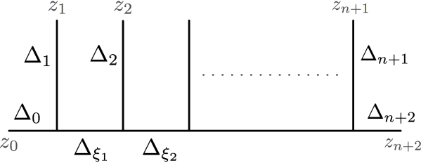
Figure 6: Pair-of-pants decomposition of the spherical conformal block with $(n+3)$ punctures

Furthermore, we take the degenerate limit in which the $(n+3)$-punctured sphere reduces to a sequence of $(n+1)$ 3-punctured spheres connected by $n$ long thin tubes with sewing parameters $q_{i}$, as shown in Fig. 7. If we denote the local coordinates on each 3-sphere by $w_{i}$, then the sewing procedure requires that

$$\frac{w_{i+1}}{w_{i}}=q_{i}\quad\mbox{with}~{}~{}|q_{i}|<0~{}.$$ (5.3)

In the local coordinates of each sphere, the punctures are located at $(0,1,\infty)$; in particular all the unsewn external punctures are at $1$ (except for the first and the last one which are at $0$ and $\infty$ respectively). However, if we use the local coordinates of the last sphere as coordinates for the global surface, the sewing relations (5.3) imply that the external punctures of the first $n$ spheres are at

$$t_{i}=\prod_{j=i}^{n}q_{j}\qquad\text{for}\qquad i\in\{1,\ldots n\}~{}.$$ (5.4)

This is precisely the same relation we found in (2.12).

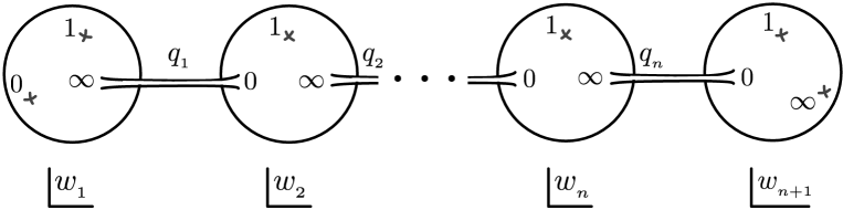
Figure 7: Three-punctured spheres connected by long thin tubes, with sewing parameters $q_{i}$.

When written in terms of the $t_{i}$’s, the conformal block (5.1) becomes [67]

$$\Big{\langle}V_{\alpha_{0}}(0)\,\prod_{i=1}^{n}V_{\alpha_{i}}(t_{i})\,V_{\alpha_{n+1}}(1)\,V_{\alpha_{n+2}}(\infty)\Big{\rangle}_{\{\xi_{1},\ldots,\xi_{n}\}}=\mathcal{N}\,\mathcal{B}(t_{i},\Delta_{\alpha_{i}},\Delta_{\xi_{i}})$$ (5.5)

where the prefactor

$$\mathcal{N} =t_{1}^{-\Delta_{\alpha_{0}}-\Delta_{\alpha_{1}}+\Delta_{\xi_{1}}}\,\prod_{i=2}^{n}t_{i}^{-\Delta_{\xi_{i-1}}-\Delta_{\alpha_{i}}+\Delta_{\xi_{i}}}\,=\,t_{1}^{-\Delta_{\alpha_{0}}}\,\prod_{i=i}^{n}t_{i}^{-\Delta_{\alpha_{i}}}q_{i}^{\Delta_{\xi_{i}}}$$ (5.6)

originates from the conformal transformations that move the vertices $V_{\alpha_{i}}$ from 1 to $t_{i}$, while $\mathcal{B}(t_{i},\Delta_{\alpha_{i}},\Delta_{\xi_{i}})$ contains all other relevant information, including the structure function coefficients and the contribution of all descendants in the internal legs.

According to [7], it is possible to establish a correspondence between the conformal block (5.5) and the partition function of the $\epsilon$-deformed $\mathrm{SU}(2)^{n}$ quiver theory. To do so, one has to identify $q_{i}$ with the gauge coupling of the $i$-th group factor, set

$$Q=\frac{\epsilon_{1}+\epsilon_{2}}{\sqrt{\epsilon_{1}\epsilon_{2}}}\,,$$ (5.7)

and choose the Liouville momenta as follows:

$$\alpha_{0} =\frac{Q}{2}+\frac{m_{1}-m_{2}}{2\sqrt{\epsilon_{1}\epsilon_{2}}}~{},\qquad\alpha_{1}=\frac{Q}{2}+\frac{m_{1}+m_{2}}{2\sqrt{\epsilon_{1}\epsilon_{2}}}~{},$$ (5.8)

$$\alpha_{i} =\frac{Q}{2}-\frac{m_{i-1,i}}{\sqrt{\epsilon_{1}\epsilon_{2}}}\qquad\mbox{for}~{}i=2,\ldots,n~{},$$

$$\xi_{i} =\frac{Q}{2}-\frac{a_{i}}{\sqrt{\epsilon_{1}\epsilon_{2}}}\,\qquad\mbox{for}~{}i=1,\ldots,n~{},$$

$$\alpha_{n+1} =\frac{Q}{2}-\frac{m_{3}+m_{4}}{2\sqrt{\epsilon_{1}\epsilon_{2}}}~{},\qquad\alpha_{n+2}=\frac{Q}{2}-\frac{m_{3}-m_{4}}{2\sqrt{\epsilon_{1}\epsilon_{2}}}~{},$$

where the $m$’s are the fundamental or bi-fundamental masses of the matter hypermultiplets as discussed in the previous sections, and $a_{i}$ is the vacuum expectation value of the adjoint scalar of the $i$-th gauge group. From (5.2) and (5.8) one can check that the conformal dimensions of the various operators are

$$\Delta_{\alpha_{0}} =\frac{(\epsilon_{1}+\epsilon_{2})^{2}-(m_{1}-m_{2})^{2}}{4\epsilon_{1}\epsilon_{2}}~{},\qquad\Delta_{\alpha_{1}}=\frac{(\epsilon_{1}+\epsilon_{2})^{2}-(m_{1}+m_{2})^{2}}{4\epsilon_{1}\epsilon_{2}}~{},$$ (5.9)

$$\Delta_{\alpha_{i}} =\frac{(\epsilon_{1}+\epsilon_{2})^{2}-4m_{i-1,i}^{2}}{4\epsilon_{1}\epsilon_{2}}\qquad\mbox{for}~{}i=2,\ldots,n~{},$$

$$\Delta_{\xi_{i}} =\frac{(\epsilon_{1}+\epsilon_{2})^{2}-4a_{i}^{2}}{4\epsilon_{1}\epsilon_{2}}~{}~{}\quad\qquad\mbox{for}~{}i=1,\ldots,n~{},$$

$$\ \Delta_{\alpha_{n+1}} =\frac{(\epsilon_{1}+\epsilon_{2})^{2}-(m_{3}+m_{4})^{2}}{4\epsilon_{1}\epsilon_{2}}~{},\qquad\Delta_{\alpha_{n+2}}=\frac{(\epsilon_{1}+\epsilon_{2})^{2}-(m_{3}-m_{4})^{2}}{4\epsilon_{1}\epsilon_{2}}~{}.$$

The remarkable observation of [7] is that

$$\mathcal{B}(t_{i},\Delta_{\alpha_{i}},\Delta_{\xi_{i}})=Z_{\mathrm{U(1)}}~{}\mathrm{e}^{-\frac{F_{\mathrm{inst}}}{\epsilon_{1}\epsilon_{2}}}~{},$$ (5.10)

where $F_{\mathrm{inst}}$ is the Nekrasov instanton prepotential and $Z_{\mathrm{U(1)}}$ ensures the correct decoupling of the U(1) factors. This U(1) contribution can be explicitly computed (see for example [67]) and the result is

$$Z_{\mathrm{U(1)}}=\prod_{i=1}^{n}\prod_{j=i+1}^{n+1}\left(1-\frac{t_{i}}{t_{j}}\right)^{-2\alpha_{i}(Q-\alpha_{j})}=\prod_{i=1}^{n}\prod_{j=i+1}^{n+1}\left(1-q_{i}\ldots q_{j-1}\right)^{-2\alpha_{i}(Q-\alpha_{j})}~{}.$$ (5.11)

The structure of these U(1) terms is actually quite simple: each factor in (5.11) can be associated to a connected subdiagram with four legs that is obtained by grouping together adjacent nodes of the quiver; the Liouville momenta of the two resulting inner legs determine the exponent [7]. For example, for $n=1$ we have just one diagram with one node and coupling constant $q$; its inner legs carry momenta $\alpha_{1}$ and $\alpha_{2}$, and the corresponding U(1) factor is

$$(1-q)^{-2\alpha_{1}(Q-\alpha_{2})}~{}.$$ (5.12)

For $n=2$ we have a subdiagram corresponding to the first node with coupling constant $q_{1}$ and inner legs with momenta $\alpha_{1}$ and $\alpha_{2}$; a subdiagram with coupling constant $q_{2}$ and inner legs carrying momenta $\alpha_{2}$ and $\alpha_{3}$, and finally a diagram with the two nodes combined, which has coupling $q_{1}q_{2}$ and inner legs with momenta $\alpha_{1}$ and $\alpha_{3}$. Thus the U(1) dressing factor is

$$(1-q_{1})^{-2\alpha_{1}(Q-\alpha_{2})}\,(1-q_{2})^{-2\alpha_{2}(Q-\alpha_{3})}\,(1-q_{1}q_{2})^{-2\alpha_{1}(Q-\alpha_{3})}~{}.$$ (5.13)

This structure, which can be easily generalized to higher values of $n$, bears a clear resemblance with that of the symmetry factors introduced in Sections 3 and 4 in the redefinition of $\widehat{F}$ (see in particular (3.7) and (4.17)). In fact, the U(1) terms (5.11) can be considered as the proper generalization in the $\epsilon$-deformed theory of the symmetry factors discussed in the previous sections. Finally, combining (5.5) and (5.10), we can write

$$\Big{\langle}V_{\alpha_{0}}(0)\,\prod_{i=1}^{n}V_{\alpha_{i}}(t_{i})\,V_{\alpha_{n+1}}(1)\,V_{\alpha_{n+2}}(\infty)\Big{\rangle}_{\{\xi_{1},\ldots,\xi_{n}\}}=\mathrm{e}^{-\frac{\widetilde{F}(\epsilon)}{\epsilon_{1}\epsilon_{2}}}$$ (5.14)

where

$$\widetilde{F}(\epsilon)=-\epsilon_{1}\epsilon_{2}\log\mathcal{N}-\epsilon_{1}\epsilon_{2}\log Z_{\mathrm{U}(1)}+F_{\mathrm{inst}}~{}.$$ (5.15)

5.2 The UV curve

The 2-dimensional Liouville theory also contains information about the SW curve of the 4-dimensional quiver gauge theory and its quantum deformation. To see this let us consider the normalized conformal block (5.5) with the insertion of the energy momentum tensor, namely

$$\phi^{\epsilon}_{2}(z)=\frac{\Big{\langle}V_{\alpha_{0}}(0)\prod_{i=1}^{n}\!V_{\alpha_{i}}(t_{i})\,T(z)\,V_{\alpha_{n+1}}(1)V_{\alpha_{n+2}}(\infty)\Big{\rangle}}{\Big{\langle}V_{\alpha_{0}}(0)\prod_{i=1}^{n}\!V_{\alpha_{i}}(t_{i})V_{\alpha_{n+1}}(1)V_{\alpha_{n+2}}(\infty)\Big{\rangle}}$$ (5.16)

with $|z|<1$. As shown in Appendix D, using the conformal Ward identities it is possible to rewrite $\phi^{\epsilon}_{2}(z)$ as

$$\phi^{\epsilon}_{2}(z)= \,\frac{\Delta_{\alpha_{0}}}{z^{2}}+\sum_{i=1}^{n}\frac{\Delta_{\alpha_{i}}}{(z-t_{i})^{2}}+\frac{\Delta_{\alpha_{n+1}}}{(z-1)^{2}}-\frac{\Delta_{\alpha_{0}}+\sum_{i=1}^{n}\Delta_{\alpha_{i}}+\Delta_{\alpha_{n+1}}-\Delta_{\alpha_{n+2}}}{z(z-1)}$$ (5.17)

$$+\sum_{i=1}^{n}\frac{t_{i}(t_{i}-1)}{z(z-1)(z-t_{i})}\frac{\partial}{\partial t_{i}}\log\Big{\langle}V_{\alpha_{0}}(0)\prod_{i=1}^{n}\!V_{\alpha_{i}}(t_{i})V_{\alpha_{n+1}}(1)V_{\alpha_{n+2}}(\infty)\Big{\rangle}~{}.$$

All terms on the right hand side of this equation are proportional to $1/(\epsilon_{1}\epsilon_{2})$ since both the conformal dimensions $\Delta$’s and the logarithm of the conformal block scale in that manner. Thus the following limit

$$\lim_{\epsilon_{1},\epsilon_{2}\rightarrow 0}\big{[}-\epsilon_{1}\epsilon_{2}\,\phi^{\epsilon}_{2}(z)\big{]}\,\equiv\,\phi_{2}(z)$$ (5.18)

is well-defined and non-singular. In this limit only the mass dependent terms of the conformal weights contribute so that one finds

$$\phi_{2}(z)= \,\frac{(m_{1}-m_{2})^{2}}{4z^{2}}+\frac{(m_{1}+m_{2})^{2}}{4(z-t_{1})^{2}}+\sum_{i=2}^{n}\frac{m^{2}_{i-1,i}}{(z-t_{i})^{2}}+\frac{(m_{3}+m_{4})^{2}}{4(z-1)^{2}}$$ (5.19)

$$-\frac{m_{1}^{2}+m_{2}^{2}+2m_{3}m_{4}+2\sum_{i=2}^{n}m^{2}_{i-1,i}}{2z(z-1)}+\sum_{i=1}^{n}\frac{t_{i}(t_{i}-1)}{z(z-1)(z-t_{i})}\frac{\partial{\widetilde{F}}}{\partial t_{i}}$$

where

$$\widetilde{F}=\lim_{\epsilon_{1},\epsilon_{2}\rightarrow 0}\widetilde{F}(\epsilon)~{}.$$ (5.20)

$\phi_{2}(z)$ has the same form of $x^{2}(z)$ appearing in the expression of the SW curve of the quiver theories described in the previous sections (see for example (3.3) or (4.13)). Indeed the mass terms are exactly the ones needed to produce the correct residues of the SW differential and coincide with those we have written for the single node and the two-node quivers in Sections 3 and 4. Also the other terms have the right structure, and thus what remains to be checked is whether the function $\widetilde{F}$ in (5.19) coincides with the analogous quantity appearing in the SW curve. We now do this check in the three cases we have analyzed in more detail.

$\bullet$ The SU(2) theory with $N_{f}=4$

For the SU(2) theory with $N_{f}=4$ things are particularly simple, since in this case there is only a non-trivial puncture at $t_{1}=q$ and $\widetilde{F}$ defined in (5.20) becomes

$$\widetilde{F}=a^{2}\log q-\frac{1}{2}(m_{1}^{2}+m_{2}^{2})\log q+\frac{1}{2}(m_{1}+m_{2})(m_{3}+m_{4})\log(1-q)+F_{\text{inst}}~{}.$$ (5.21)

Using (3.5) and (3.7), one can immediately see that this agrees with the function $\widetilde{F}$ appearing in the SW curve (3.3).

$\bullet$ The SU(2)$\,\times\,$SU(2) quiver theory

In the 2-node quiver there are two non-trivial punctures. In the above discussion we have located them at $t_{1}=q_{1}q_{2}$ and $t_{2}=q_{2}$, while in the curve derivation of Section 4 we have considered a different (though completely equivalent) configuration with punctures at $t_{1}=q_{1}$ and $t_{2}=1/q_{2}$. Thus, before comparing we have to make the appropriate changes in the prefactor $\mathcal{N}$ which, being directly connected to the factorization of the conformal block in pair-of-pants diagrams, crucially depends on where the non-trivial punctures are located. If we set the punctures at $t_{1}=q_{1}$ and $t_{2}=1/q_{2}$, we have to use

$$\mathcal{N}=q_{1}^{-\Delta_{\alpha_{0}}-\Delta_{\alpha_{1}}+\Delta_{\xi_{1}}}\,q_{2}^{\Delta_{\xi_{2}}+\Delta_{\alpha_{2}}-\Delta_{\alpha_{3}}}~{}.$$ (5.22)

The corresponding expression for $\widetilde{F}$ is then

$$\widetilde{F}= \,a_{1}^{2}\log q_{1}+a_{2}^{2}\log q_{2}-\frac{1}{2}(m_{1}^{2}+m_{2}^{2})\log q_{1}+m_{3}m_{4}\log q_{2}$$ (5.23)

$$+m_{12}(m_{1}+m_{2})\log(1-q_{1})-m_{12}(m_{3}+m_{4})\log(1-q_{2})$$

$$+\frac{1}{2}(m_{1}+m_{2})(m_{3}+m_{4})\log(1-q_{1}q_{2})+F_{\text{inst}}~{},$$

which exactly matches the one appearing in the M-theory derivation of the SW curve, as one can see using (4.15) and (4.17). This same result can also be obtained from the general expression (5.19) if we notice that under the change of variables that maps $(q_{1}q_{2},q_{2},1)$ to $(q_{1},1,1/q_{2})$, the term of $\phi_{2}(z)$ proportional to $1/(z(z-1)$ produces an extra contribution to $\widetilde{F}$ modifying its expression and leading to (5.23).

$\bullet$ The conformal $\mathrm{SU}(2)^{n}$ quiver

When all masses are zero, ${\widetilde{F}}$ in (5.20) is simply

$$\widetilde{F}=\sum_{i=1}^{N}a_{i}^{2}\,\log q_{i}+F_{\text{inst}}\,.$$ (5.24)

Up to 1-loop $t$-independent contributions, this is precisely the prepotential $F$ of the conformal quiver gauge theory, and thus the corresponding SW curve can be written as

$$\phi_{2}(z)=\sum_{i=1}^{n}\frac{t_{i}(t_{i}-1)}{z(z-1)(z-t_{i})}\frac{\partial{F}}{\partial t_{i}}~{},$$ (5.25)

confirming in this case the direct identification of the residues at $t_{i}$ with the derivatives of the gauge theory prepotential [47, 48]. We can therefore say that the AGT correspondence provides the analogue of the Matone relations [46] for the quiver gauge theory. One can go even further and map the curve (5.25) to that in (2.27) obtained using the M-theory analysis, thus finding the explicit relation between the Coulomb parameters $u_{i}$ appearing there and the $t_{i}$-derivatives of the prepotential.

6 The quiver prepotential from null-vector decoupling

We now present the derivation of the $\Omega$-deformed prepotential for the $\mathrm{SU}(2)^{n}$ quiver model in the NS limit [6] using a null-vector decoupling equation in the Liouville theory introduced in the previous section. The observable we consider is the conformal block obtained by deforming (5.5) with the insertion of the degenerate field $\Phi_{2,1}(z)$ of the Virasoro algebra [8], namely

$$\Psi(z)=\Big{\langle}V_{\alpha_{0}}(0)\,\prod_{i=1}^{n}V_{\alpha_{i}}(t_{i})\,\Phi_{2,1}(z)\,V_{\alpha_{n+1}}(1)\,V_{\alpha_{n+2}}(\infty)\Big{\rangle}_{\{\xi_{1},\ldots,\xi_{n}\}}$$ (6.1)

with $|z|<1$. The degenerate field $\Phi_{2,1}$ has conformal dimension

$$\Delta_{2,1}=-\frac{1}{2}-\frac{3}{4}\,\frac{\epsilon_{2}}{\epsilon_{1}}$$ (6.2)

and satisfies the null-vector condition

$$\frac{\epsilon_{1}}{\epsilon_{2}}\,\frac{d^{2}\Phi_{2,1}(z)}{dz^{2}}\,+\,:\!T(z)\Phi_{2,1}(z)\!:\,=0~{}.$$ (6.3)

This condition implies that $\Psi(z)$ obeys a second order differential equation that can be obtained from the conformal Ward identities as discussed in Appendix D. If we normalize the correlator (6.1) with the unperturbed one (5.14) and write

$$\Psi(z)=\mathrm{e}^{-\frac{\widetilde{F}(\epsilon)}{\epsilon_{1}\epsilon_{2}}}\,\Phi(z)~{},$$ (6.4)

then the differential equation for $\Psi(z)$ turns into the following differential equation for $\Phi(z)$

$$\Bigg{[}\frac{\epsilon_{1}}{\epsilon_{2}}\frac{\partial^{2}}{\partial z^{2}}-\frac{2z-1}{z(z-1)}\frac{\partial}{\partial z}+\sum_{i=1}^{n}\Big{(}\frac{t_{i}(t_{i}-1)}{z(z-1)(z-t_{i})}\frac{\partial}{\partial t_{i}}-\frac{1}{\epsilon_{1}\epsilon_{2}}\,\frac{t_{i}(t_{i}-1)}{z(z-1)(z-t_{i})}\frac{\partial{\widetilde{F}(\epsilon)}}{\partial t_{i}}\Big{)}+\frac{\Delta_{\alpha_{0}}}{z^{2}}$$ (6.5)

$$+\sum_{i=1}^{n}\frac{\Delta_{\alpha_{i}}}{(z-t_{i})^{2}}+\frac{\Delta_{\alpha_{n+1}}}{(z-1)^{2}}-\frac{\Delta_{\alpha_{0}}+\sum_{i=1}^{n}\Delta_{\alpha_{i}}+\Delta_{2,1}+\Delta_{\alpha_{n+1}}-\Delta_{\alpha_{n+2}}}{z(z-1)}\Bigg{]}\,\Phi(z)~{}=0~{}.$$

This equation is well-suited to take the NS limit [6] in which $\epsilon_{2}\to 0$ with $\epsilon_{1}\not=0$, provided we assume that

$$\Phi(z)=\mathrm{e}^{-\frac{W(z)}{\epsilon_{1}}}$$ (6.6)

where $W(z)$ is regular in $\epsilon_{1}$. Multiplying (6.5) by $(-\epsilon_{1}\epsilon_{2})$ and sending $\epsilon_{2}$ to zero, the differential equation simplifies in a few ways: the linear derivatives in $z$ and $t_{i}$ drop out along with the term proportional to the conformal dimension $\Delta_{2,1}$ of the degenerate field. Furthermore, in the NS limit the generalized prepotential $\widetilde{F}(\epsilon)$ in (5.15) becomes

$$\widetilde{F}(\epsilon)\,\to\,\widetilde{F}+\epsilon_{1}\widetilde{F}^{(1)}+\epsilon_{1}^{2}\widetilde{F}^{(2)}$$ (6.7)

where the $\epsilon_{1}$ corrections arise from the explicit $\epsilon$-dependence of the prefactors $\mathcal{N}$ and $Z_{\mathrm{U}(1)}$. Since the terms proportional to the conformal dimensions $\Delta_{\alpha_{i}}$ yield contributions at most of order $\epsilon_{1}^{2}$, in the end we obtain the Schroedinger-type differential equation:

$$\Big{(}-\epsilon_{1}^{2}\frac{d^{2}}{dz^{2}}+V(z,\epsilon_{1})\Big{)}\Phi(z)=0~{},$$ (6.8)

where

$$V(z,\epsilon_{1})=V^{(0)}(z)+\epsilon_{1}\,V^{(1)}(z)+\epsilon_{1}^{2}\,V^{(2)}(z)$$ (6.9)

with

$$V^{(0)}(z) = \phi_{2}(z)~{},$$

$$V^{(1)}(z) = \sum_{i=1}^{n}\,\frac{t_{i}(t_{i}-1)}{z(z-1)(z-t_{i})}\frac{\partial\widetilde{F}^{(1)}}{\partial t_{i}}~{},$$ (6.10)

$$V^{(2)}(z) = -\frac{1}{4z^{2}}-\sum_{i=1}^{n}\frac{1}{4(z-t_{i})^{2}}-\frac{1}{4(z-1)^{2}}+\frac{n+1}{4z(z-1)}+\sum_{i=1}^{n}\,\frac{t_{i}(t_{i}-1)}{z(z-1)(z-t_{i})}\frac{\partial\widetilde{F}^{(2)}}{\partial t_{i}}~{}.$$

Note that $V^{(0)}$ is the SW curve of the undeformed theory. To solve (6.8) we make a WKB-like ansatz for $\Phi(z)$ writing

$$W(z)=\int^{z}\!\!P(z^{\prime},\epsilon_{1})\,dz^{\prime}~{},$$ (6.11)

and then expand $P$ in powers of $\epsilon_{1}$

$$P(z,\epsilon_{1})=\sum_{n=0}^{\infty}\epsilon_{1}^{n}\,P^{(n)}(z)~{}.$$ (6.12)

Substituting in (6.8) we find

$$-P(z,\epsilon_{1})^{2}+\epsilon_{1}\frac{dP(z,\epsilon_{1})}{dz}+V(z,\epsilon_{1})=0~{},$$ (6.13)

which in turn can be solved perturbatively in $\epsilon_{1}$. The first few terms are

$$P^{(0)}(z) =\sqrt{\phi_{2}(z)}~{},$$ (6.14a)

$$P^{(1)}(z) =\frac{1}{2}\frac{d}{dz}\log P^{(0)}(z)+\frac{V^{(1)}(z)}{2P^{(0)}(z)}~{},$$ (6.14b)

$$P^{(2)}(z) =\frac{{P^{(1)}}^{\prime}(z)-{P^{(1)}}^{2}(z)}{2P^{(0)}(z)}+\frac{V^{(2)}(z)}{2P^{(0)}(z)}~{},$$ (6.14c)

and so on. Since $P^{(0)}(z)dz$ is simply the SW differential of the undeformed theory, it is more than natural to define the deformed SW differential as

$$\lambda(\epsilon_{1})=P(z,\epsilon_{1})\,dz~{}.$$ (6.15)

The periods of $\lambda(\epsilon_{1})$ along the $\alpha_{i}$-cycles can then be interpreted as the $a_{i}$’s in the deformed theory, namely

$$a_{i}=\frac{1}{2\pi\mathrm{i}}\oint_{\alpha_{i}}\!\lambda(\epsilon_{1})=\sum_{n=0}^{\infty}\epsilon_{1}^{n}\,a_{i}^{(n)}\qquad\mbox{with}\qquad a_{i}^{(n)}=\frac{1}{2\pi\mathrm{i}}\oint_{\alpha_{i}}\!P^{(n)}(z)\,dz~{}.$$ (6.16)

Clearly the above integrals depend on the prepotential $F$ and its $t_{i}$-derivatives; therefore we can use this information to fix the $\epsilon_{1}$-dependence of $F$ by demanding consistency, namely by choosing $a_{i}$’s as independent variables and thus taking them to be constant. Even if it does not seem so at first sight, this procedure is fully equivalent to that used for instance in [54, 55] to obtain the deformed prepotential for the $\mathcal{N}=2^{*}$ SU(2) theory or the $\mathcal{N}=2$ SU(2) theory with $N_{f}=4$. Indeed, also in our case the periods $a_{i}$ which determine the monodromy properties of the wave function $\Phi(z)$, are constant, since the $\epsilon_{1}$ (and $q_{i}$) dependence of the prepotential is fixed precisely to achieve this goal. It is remarkable that the prepotential obtained in this way agrees with the one computed using localization methods in the NS limit.

6.1 The prepotential from deformed period integrals

We now illustrate the above procedure, focusing on the examples considered in the previous sections.

$\bullet$ The SU$(2)$ theory with $N_{f}=4$

When $n=1$, the $\epsilon_{1}$-terms of the potential in the Schroedinger-type equation are

$$V^{(1)}(z) =q\,\frac{(m_{1}+m_{2}+m_{3}+m_{4})}{2z(z-q)(z-1)}~{},$$ (6.17)

$$V^{(2)}(z) =-\frac{1}{4z^{2}}-\frac{1}{4(z-q)^{2}}-\frac{1}{4(z-1)^{2}}+\frac{1}{2z(z-1)}+\frac{3q-1}{4z(z-1)(z-q)}~{},$$

while $V^{(0)}(z)$ is given by the SW curve $\phi_{2}(z)$.

To proceed we choose the same mass configuration that we have discussed in Section 3, namely $m_{1}=m_{2}=m$, $m_{3}=m_{4}=M$, which allows us to write the curve in the factorized form

$$\phi_{2}(z)=\frac{C(e_{2}-z)(z-e_{3})}{z(z-1)^{2}(z-q)^{2}}~{}.$$ (6.18)

Here the roots $e_{2}$ and $e_{3}$ and the constant $C$ are the same as in (3.14) and (3.15), but they are expressed in terms of the prepotential instead of the Coulomb modulus $u$.

At order $\epsilon_{1}^{0}$, the period has already been calculated in Section 3 (see (3.20)); expressing it in terms of $U\equiv q\,\partial F/\partial q$, we have (up to 2 instantons)

$$a^{(0)} = \sqrt{U}\,\bigg{[}1-\frac{q}{4}\Big{(}1+\frac{(m^{2}+4mM+M^{2})}{U}+\frac{m^{2}M^{2}}{U^{2}}\Big{)}$$ (6.19)

$$~{}-\frac{q^{2}}{64}\Big{(}7\!+\!\frac{14m^{2}+48mM+14M^{2}}{U}\!+\!\frac{3m^{4}+16m^{3}M+60m^{2}M^{2}+16mM^{3}+3M^{4}}{U^{2}}$$

$$~{}+\frac{6m^{2}M^{2}(m^{2}+8mM+M^{2})}{U^{3}}+\frac{15m^{4}M^{4}}{U^{4}}\Big{)}+\ldots\bigg{]}~{}.$$

At order $\epsilon_{1}$ we have instead

$$a^{(1)}=\frac{1}{2\pi\mathrm{i}}\oint_{\alpha}P^{(1)}(z)\,dz=-q\,\frac{m+M}{2\pi\sqrt{C}}\int_{0}^{e_{2}}\frac{dz}{\sqrt{z(e_{2}-z)(e_{3}-z)}}$$ (6.20)

where in the second step we used (6.14b) and discarded the total derivative term. This integral can be evaluated as a power series and, up to two instantons, we find

$$a^{(1)}=-q\,\frac{m+M}{2\sqrt{U}}\bigg{[}1+q\,\frac{3U^{2}+U(m^{2}+4mM+M^{2})+3m^{2}M^{2}}{4U^{2}}+\ldots\bigg{]}~{}.$$ (6.21)

Using the formulæ in (6.14) iteratively, we can easily compute the order $\epsilon_{1}^{2}$ correction to the period and get

$$a^{(2)}= -\frac{q}{16U^{\frac{5}{2}}}\bigg{[}3U^{2}+m^{2}M^{2}+\frac{q}{8U^{2}}\Big{(}17U^{4}+7U^{3}(3m^{2}+8mM+3M^{2})$$ (6.22)

$$+2U^{2}(m^{4}+20m^{2}M^{2}+M^{4})-5Um^{2}M^{2}(m^{2}-8mM+M^{2})+35m^{4}M^{4}\Big{)}+\ldots\bigg{]}~{}.$$

So far, we have calculated the period integral as an expansion of the form

$$a=a^{(0)}(U)+\epsilon_{1}\,a^{(1)}(U)+\epsilon_{1}^{2}\,a^{(2)}(U)+\ldots$$ (6.23)

We now invert this expression and determine how $U$ should depend on $\epsilon_{1}$ so that $a$ be a constant. We can do this by writing

$$U=U^{(0)}+\epsilon_{1}\,U^{(1)}+\epsilon_{1}^{2}\,U^{(2)}+\ldots$$ (6.24)

and demanding consistency order by order in $\epsilon_{1}$. Once $U$ is computed, we can obtain the deformed prepotential $F$ by integrating it with respect to (the logarithm of) $q$. The zeroth-order term that we get in this way clearly coincides with (3.22), while the first successive corrections are given by

$$F^{(1)} =q\,(m+M)+\frac{q^{2}}{2}\,(m+M)+\ldots~{},$$ (6.25)

$$F^{(2)} =\frac{q}{8}\Big{(}3+\frac{m^{2}M^{2}}{a^{4}}\Big{)}+\frac{q^{2}}{128}\Big{(}23-\frac{m^{2}+M^{2}}{a^{2}}+\frac{2m^{4}+16m^{2}M^{2}+2M^{4}}{a^{4}}$$

$$\hskip 142.26378pt-\frac{15m^{2}M^{2}(m^{2}+M^{2})}{a^{6}}+\frac{21m^{4}M^{4}}{a^{8}}\Big{)}+\ldots$$

These precisely match the microscopic results obtained from the Nekrasov partition function via localization methods.

$\bullet$ The SU$(2)\times$ SU$(2)$ quiver theory

When $n=2$ the Schroedinger problem is algebraically more complicated, but still doable. The $\epsilon_{1}$-corrections of the potential $V$ are

$$V^{(1)}(z)= \frac{(m_{1}+m_{2}+m_{3}+m_{4})q_{1}q_{2}}{2z(z-1)(z-q_{1}q_{2})}+\frac{(m_{1}+m_{2}+2m_{12})q_{1}q_{2}}{2z(z-q_{2})(z-q_{1}q_{2})}+\frac{(m_{3}+m_{4}-2m_{12})q_{2}}{2z(z-1)(z-q_{2})}~{},$$ (6.26)

$$V^{(2)}(z)= -\frac{1}{4z^{2}}-\frac{1}{4(z-q_{1}q_{2})^{2}}-\frac{1}{4(z-q_{2})^{2}}-\frac{1}{4(z-1)^{2}}+\frac{3}{4z(z-1)}$$

$$\qquad\quad-\frac{\eta_{1}}{z(z-1)(z-q_{2})}-\frac{\eta_{2}}{z(z-q_{2})(z-q_{1}q_{2})}$$

where

$$\eta_{1}=\frac{(1-2(1+q_{1})q_{2}+3q_{1}q_{2}^{2})}{2(1-q_{1}q_{2})}~{},\qquad\eta_{2}=\frac{q_{2}(1+5q_{1}^{2}q_{2}-3q_{1}(1+q_{2}))}{4(1-q_{1}q_{2})}~{}.$$ (6.27)

To proceed we make the simplifying mass choices discussed in Section 4, see (4.22).

Case A):

In our present conventions the SW curve takes the factorized form

$$\phi_{2}(z)=\frac{-u_{2}(z-q_{2}\zeta_{1})(z-q_{2}\widehat{\zeta})}{z(z-1)(z-q_{1}q_{2})^{2}(z-q_{2})}$$ (6.28)

where the various constants are exactly those appearing in (4.24), with the $u_{i}$’s written in terms of the $U_{i}$’s using (4.27). Furthermore, with this mass choice the first-order term of the potential simplifies to

$$V^{(1)}(z)=-\frac{mq_{1}q_{2}(1+q_{2}-2z)}{z(z-1)(z-q_{2})(z-q_{1}q_{2})}~{}.$$ (6.29)

Using the same basis of $\alpha$-cycles discussed in Section 4, we find that the first correction to the $a_{1}$-period takes the form

$$a_{1}^{(1)} =\frac{1}{2\pi\mathrm{i}}\oint_{\alpha_{1}}\!\!P^{(1)}(z)\,dz=-\frac{mq_{1}q_{2}}{2\sqrt{u_{2}}}\int_{0}^{q_{2}\zeta_{1}}\!\!\!\frac{dz}{\sqrt{z(q_{2}\zeta_{1}-z)}}\,\frac{(1+q_{2}-2z)}{\sqrt{(1-z)(q_{2}-z)(q_{2}\widehat{\zeta}-z)}}~{}.$$ (6.30)

Note that, unlike the case of the undeformed period (4.29), now there are no poles in the integrand and the integral can be done simply by expanding the second factor of (6.30) in powers of $z$ and writing the resulting integrals in terms of Euler $\beta$-functions. In this way we find

$$a_{1}^{(1)}= -\frac{mq_{1}}{2\sqrt{U_{1}\phantom{|}}}\bigg{[}1-q_{1}\frac{U_{1}(U_{2}-3U_{1})+m^{2}(3U_{2}-U_{1})}{4U_{1}^{2}}+q_{2}+\ldots\bigg{]}~{}.$$ (6.31)

The first correction to the $a_{2}$ period can be similarly performed and we obtain

$$a_{2}^{(1)}=-\frac{3m\,q_{1}q_{2}}{4\sqrt{U_{2}\phantom{|}}}+\ldots~{}.$$ (6.32)

At order $\epsilon_{1}^{2}$ we find

$$a_{1}^{(2)} = -\frac{q_{1}}{16\,U_{1}^{\frac{5}{2}}}\bigg{[}3U_{1}^{2}-m^{2}U_{2}\!-q_{2}\Big{(}5U_{1}^{2}+m^{2}(U_{1}+U_{2})\Big{)}\!-\frac{q_{1}}{8}\Big{(}17U_{1}^{2}-7U_{1}U_{2}+2U_{2}^{2}$$ (6.34)

$$\phantom{\Bigg{|}}~{}~{}+\frac{m^{2}(21U_{1}^{2}-24U_{1}U_{2}-5U_{2}^{2})}{U_{1}}+\frac{m^{4}(2U_{1}^{2}-25U_{1}U_{2}+35U_{2}^{2})}{U_{1}^{2}}\Big{)}+\ldots\bigg{]}~{},$$

$$a_{2}^{(2)} = -\frac{q_{2}}{16\sqrt{U_{2}\phantom{|}}}\bigg{[}3+5q_{1}+q_{2}\frac{2U_{1}^{2}-7U_{1}U_{2}+17U_{2}^{2}}{8U_{1}^{2}}+\ldots\bigg{]}~{}.$$ (6.35)

Inverting the expansion of the periods order-by-order in $\epsilon_{1}$, we can determine the $\epsilon_{1}$ dependence of $U_{1}$ and $U_{2}$. At each order the resulting expressions turn out to be integrable and the prepotential can be recovered. At order $\epsilon_{1}^{0}$ we get the same expression as in (4.1), while the corrections of order $\epsilon_{1}$ and $\epsilon_{1}^{2}$ are

$$F^{(1)} = m\bigg{(}q_{1}+\frac{1}{2}q_{1}^{2}+q_{1}q_{2}+\ldots\bigg{)}~{},$$ (6.36)

$$F^{(2)} = q_{1}\,\frac{3a_{1}^{4}-m^{2}a_{2}^{2}}{8a_{1}^{4}}+q_{2}\,\frac{3}{8}+q_{1}q_{2}\,\frac{7a_{1}^{4}+m^{2}a_{2}^{2}}{16a_{1}^{4}}+q_{2}^{2}\,\frac{23a_{2}^{4}-a_{1}^{2}a_{2}^{2}+2a_{1}^{4}}{128a_{2}^{4}}$$

$$+q_{1}^{2}\bigg{(}\frac{23a_{1}^{4}-a_{1}^{2}a_{2}^{2}+2a_{2}^{4}}{128a_{1}^{4}}-\frac{m^{2}(a_{1}^{4}+15a_{2}^{4})}{128a_{1}^{6}}+\frac{m^{4}(2a_{1}^{4}-15a_{1}^{2}a_{2}^{2}+21a_{2}^{4})}{128a_{1}^{8}}\bigg{)}+\ldots$$

One can check that this precisely matches the $\epsilon_{1}$ corrections to the prepotential obtained using Nekrasov’s analysis, thus validating the entire picture.

Case B):

The SW curve in this case is

$$\phi_{2}(z)=\frac{C(z-q_{2}\,\zeta_{3})(z-q_{2}\,\widehat{\zeta})}{z(z-q_{1}q_{2})(z-q_{2})^{2}(z-1)}$$ (6.38)

where the constants are the same as in (4.45) and (4.46), provided we write the $u_{i}$’s in terms of the $U_{i}$’s by means of (4.47). For this mass configuration, the first-order correction to the Schroedinger potential is

$$V^{(1)}(z)=-\frac{M\,q_{2}\big{(}z(1-q_{1})+q_{1}(1-q_{2})\big{)}}{z(z-q_{1}q_{2})(z-q_{2})(z-1)}~{},$$ (6.39)

and the $\alpha_{i}$-cycles are unchanged from the undeformed theory. Thus the period integrals are straightforward to perform, leading to the following results

$$a_{1}^{(1)} = \frac{1}{2\pi\mathrm{i}}\oint_{\alpha_{1}}\!\!\!P^{(1)}(z)\,dz=-\frac{Mq_{2}}{2\sqrt{C}}\int_{0}^{q_{1}q_{2}}\!\!\frac{dz}{\sqrt{z(q_{1}q_{2}-z)}}\,\frac{z(1-q_{1})+q_{1}(1-q_{2})}{\sqrt{(q_{2}\zeta_{3}-z)(q_{2}\widehat{\zeta}-z)(1-z)}}$$ (6.40)

$$= -\frac{q_{1}M}{2\sqrt{U_{1}\phantom{|}}}\bigg{[}1+q_{1}\,\frac{3U_{1}-U_{2}+M^{2}}{4U_{1}}-\frac{q_{2}}{2}+\ldots\bigg{]}~{}.$$

At order $\epsilon_{1}^{2}$ we find

$$a_{1}^{(2)}\! =\!-\frac{q_{1}}{16\sqrt{U_{1}\phantom{|}}}\bigg{[}3+5q_{2}+q_{1}\,\frac{17U_{1}^{2}-7U_{1}U_{2}+2U_{2}^{2}-M^{2}(21U_{1}-4U_{2})-2M^{4}}{8U_{1}^{2}}+\!\ldots\bigg{]}~{}.$$ (6.41)

The period integrals $a_{2}^{(k)}$ along the $\alpha_{2}$-cycle can be obtained from the above expressions by the following symmetry operations

$$U_{1}\leftrightarrow U_{2}~{},\qquad q_{1}\leftrightarrow q_{2}~{},\qquad M\leftrightarrow-M~{}.$$ (6.42)

Inverting as before the map between the $a_{i}$’s and the $U_{i}$’s, and integrating with respect to the coupling constants $q_{i}$, we find that the first $\epsilon_{1}$-corrections to the prepotential are

$$F^{(1)} =M(q_{1}-q_{2})+\frac{M}{2}(q_{1}^{2}-q_{2}^{2})+\ldots~{},$$ (6.43)

$$F^{(2)} =\frac{3(q_{1}+q_{2})}{8}+\frac{7q_{1}q_{2}}{16}+q_{1}^{2}\,\frac{23a_{1}^{4}-a_{1}^{2}a_{2}^{2}+2a_{2}^{4}-M^{2}(4a_{1}^{2}+a_{2}^{2})+2M^{4}}{128a_{1}^{4}}$$

$$\qquad+q_{2}^{2}\frac{23a_{2}^{4}-a_{1}^{2}a_{2}^{2}+2a_{1}^{4}-M^{2}(4a_{2}^{2}+a_{1}^{2})+2M^{4}}{128a_{2}^{4}}+\ldots~{}.$$

This perfectly agrees with the Nekrasov prepotential for this mass configuration.

Combining the results for the two different mass configurations with the symmetry that exchanges the two gauge groups, the associated masses and coupling constants, we can therefore claim that the results following from the null-vector decoupling equation are completely consistent with the $\Omega$-deformed prepotential obtained from localization in the NS limit.

7 Conclusions

In this paper we have considered $\mathrm{SU}(2)^{n}$ super-conformal linear quiver gauge theories, with special emphasis on the $n=1,2$ cases, comparing two different approaches: one based on the analysis of the SW curves and the other based on the AGT correspondence.

Starting from the SW curves obtained from the M-theory lift of a system of NS5-D4 branes, we have shown how to derive efficiently the instanton expansion of the prepotential. We used a generalized residue prescription, along the lines suggested in [47, 48], together with global symmetry considerations. We have also shown that the cross-ratios of the branch points of the SW curve, which depend on the UV parameters of the theory, can be expressed in terms of $\Theta$-constants with period matrix $\tau_{ij}$, which encodes the IR gauge couplings, thus confirming the nice geometric interpretation of the Nekrasov counting parameters.

We then considered the AGT correspondence, and showed that the classical SW curve encoded in this approach matches perfectly the one obtained via the M-theory analysis. Within this framework it is also possible to investigate the $\Omega$-deformed quiver theory, at least in the NS limit where the periods $a_{i}$ can be written as integrals of a deformed SW differential. From this expression we were able to extract the expansion of the prepotential to second order in the deformation parameter, which agrees completely with the microscopic evaluation of the prepotential à la Nekrasov. It is clear that our methods can be generalized in a straightforward manner to higher orders, and indeed we were able to push the calculations up to order four in a few cases.

To compare the results obtained in the two approaches, the key point is to express all parameters in terms of gauge theory data, which are the masses and the bare coupling constants associated to each gauge group. In the M-theory approach, the parameters are geometric, and are related to the positions of the constituent branes that engineer the quiver gauge theory. In the Liouville theory, the natural parameters are the central charge of the CFT and the Liouville momenta of the primary operators involved in the AGT correspondence. After working out the detailed map between the various parameters, we could correctly identify the quantum mechanical system that governs the infrared dynamics of the SU$(2)^{n}$ quiver gauge theory in the NS limit, for the cases $n=1,2$. This in turn allowed us to calculate the prepotential of the gauge theory.

There are many directions that deserve to be explored.

As mentioned in the introduction, there is a very powerful approach to the study of mass deformed conformal quiver gauge theories, which uses the limit shape equations [32, 33]. This method does not rely on the existence of an AGT dual. It has been shown that in the NS limit, the instanton partition function of the quiver gauge theory reduces to the wave function of some quantum mechanical system. It would be very interesting to analyze those differential equations using our simple techniques to see if they prove to be efficient in calculating the prepotential of the quiver theories.

In all the cases discussed in this paper, we focused on mass configurations such that the SW curve can be explicitly written in a factorized form. This allowed us to compute the period integrals using relatively simple integration techniques, so that the discussion could be focused on more conceptual issues. For generic masses, we will have to use more sophisticated methods to evaluate the period integrals.

The WKB ansatz for the wave-function which we used to obtain the deformed periods in our examples, and which is valid only in the NS limit, would clearly work for the general linear quiver with SU(2) gauge group factors. Since $\epsilon_{1}$ appears as the Planck’s constant for this quantum mechanical problem, it would be interesting to explore the presence of contributions that are non-perturbative in $\epsilon_{1}$, and explore their possible effects on the prepotential and their interpretation in the gauge theory (see [68] and references therein for some interesting recent work using exact WKB methods).

For conformal quiver theories with SU($N$) gauge groups, the AGT dual is the Toda CFT, which has a $W_{N}$ symmetry. It would be interesting to study the null-vector decoupling equations in such theories. In the NS limit, the resulting differential equation will be of higher order and it remains to be seen if there exists a suitable WKB-type ansatz for the wave function that can be used to obtain the prepotential of such quivers.

For conformal gauge theories with a single gauge group, such as $\mathrm{SU}(2)$ theory with $N_{f}=4$ and the $\mathcal{N}=2^{*}$ theory, there has been tremendous progress in resumming the instanton contributions and writing the prepotential in terms of quasi-modular functions of the coupling constant. This has been done both from the gauge theory perspective [69]-[71] as well as from the Liouville CFT perspective [54, 55, 57]. It would be interesting to see if similar resummations are possible for the general linear quiver. A related question would be to understand and interpret our results in the context of topological string theory. Both these directions require the ability to describe $\Omega$-deformations beyond the NS limit $\epsilon_{2}=0$, since the quantity $\sqrt{\epsilon_{1}\epsilon_{2}}$ plays the rôle of the string coupling constant for the related topological string theories. Moreover, the holomorphic/modular anomaly equation (which allows the resummation of instanton contributions in terms of suitable modular quantities) has its roots in a quantization of the moduli space for which $\epsilon_{1}\epsilon_{2}$ represents the Planck constant. We hope to pursue some of these directions in the future.

Acknowledgments We would like to thank Dileep Jatkar, Madhusudhan Raman, Ashoke Sen and Jan Troost for useful discussions. The work of M.B., M.F. and A.L. is partially supported by the Compagnia di San Paolo contract “MAST: Modern Applications of String Theory” TO-Call3-2012-0088.

Appendix A Nekrasov prepotential for quiver gauge theories

We consider $\mathcal{N}=2$ quiver theories with a gauge group of the form $\prod_{i}\mathrm{SU}(N_{i})$, and a matter content specified by the numbers $\{n_{i}\}$ of hypermultiplets in the fundamental representation of $\mathrm{SU}(N_{i})$, and by the numbers $\{c_{ij}\}$ of bi-fundamental hypermultiplets which are fundamental under $\mathrm{SU}(N_{i})$ and anti-fundamental under $\mathrm{SU}(N_{j})$. The $\beta$-function coefficient for each $\mathrm{SU}(N_{i})$ factor is given by

$$\beta_{i}=-2N_{i}+\sum_{j}N_{j}(c_{ij}+c_{ji})+n_{j}~{}.$$ (A.1)

We restrict our attention to conformal theories such that the $\beta$-function vanishes for every node. The basic quantity of interest is the multi-instanton partition function which, using localization [4, 5], reduces to

$$Z_{\mathrm{inst}}=\sum_{k_{i}}\,\int\prod_{i}\frac{q_{i}^{k_{i}}}{k_{i}!}\prod_{I_{i}=1}^{k_{i}}\frac{d\chi_{I_{i}}}{2\pi i}\ z^{\mathrm{quiver}}_{\{k_{i}\}}~{}.$$ (A.2)

Here we adopt the same conventions used in [27] (see in particular Appendix A). For instance, in the $(k_{1},k_{2})$ instanton sector of a 2-node quiver theory we have

$$z^{\mathrm{quiver}}_{k_{1},k_{2}}=z_{k_{1}}^{\mathrm{gauge}}\,z_{k_{2}}^{\mathrm{gauge}}\,z_{k_{1}}^{\mathrm{fund}}z_{k_{2}}^{\mathrm{fund}}\,z_{k_{1},k_{2}}^{\mathrm{bi-fund}}~{}.$$ (A.3)

where, in a rather obvious notation, the various factors represent the contributions of the different multiplets. As shown in [4, 5] (see also [35, 38]), the configurations of $\chi_{I_{i}}$ which contribute to the integrals in (A.2) can be put in one-to-one correspondence with a set Young tableaux $Y=\{Y_{i}\}$ containing a total number $k=\sum_{i}k_{i}$ of boxes, and the instanton partition function can be rewritten as

$$Z_{\mathrm{inst}}=1+\sum_{Y_{i}}\prod_{i}q_{i}^{|Y_{i}|}Z_{\{Y_{i}\}}~{}.$$ (A.4)

Here, the $1$ represents the contribution at zero instanton number, $|Y_{i}|$ is the total number of boxes of the $i$-th Young tableau.

There is an algorithmic way to calculate the $Z_{Y_{i}}$’s, using the formalism of group characters, which now we briefly describe. For a given node $i$, we introduce the characters associated to the gauge, flavour and instanton symmetries, namely:

$$W_{i}=\sum_{u_{i}=1}^{N_{i}}\mathrm{e}^{\mathrm{i}a_{u_{i}}}~{},\quad W_{F,i}=\sum_{f_{i}=1}^{n_{i}}\mathrm{e}^{-\mathrm{i}\big{(}m_{f_{i}}+\frac{1}{2}(\epsilon_{1}+\epsilon_{2})\big{)}}~{},\quad V_{i}=\sum_{I_{i}=1}^{k_{i}}\mathrm{e}^{\mathrm{i}\big{(}\chi_{I_{i}}-{\textstyle\frac{1}{2}}(\epsilon_{1}+\epsilon_{2})\big{)}}\,,$$ (A.5)

where the $m$’s are the masses of the fundamental hypermultiplets while $\epsilon_{1}$ and $\epsilon_{2}$ are the parameters of the $\Omega$-background [4, 5]. In addition to these, we also have the characters associated to the Lorentz group, which are given by

$$T_{1}=\mathrm{e}^{\mathrm{i}\epsilon_{1}}~{},\qquad T_{2}=\mathrm{e}^{\mathrm{i}\epsilon_{2}}~{}.$$ (A.6)

For a quiver model specified by the data $\{n_{i},c_{ij}\}$, the character for a given tableau $Y$ is expressed in terms of the fundamental characters (A.5) as follows:

$$T_{Y}=\sum_{i,j}t_{ij}\,T_{ij}-T_{F}\,,$$ (A.7)

with

$$t_{ij} =\delta_{ij}-c_{ij}\,\mathrm{e}^{\mathrm{i}\big{(}m_{ij}-{\textstyle\frac{1}{2}}(\epsilon_{1}+\epsilon_{2})\big{)}}~{},$$ (A.8)

$$T_{ij} =-V_{i}V^{*}_{j}(1-T_{1})(1-T_{2})+W_{i}V_{j}^{*}+V_{i}W_{j}^{*}T_{1}T_{2}~{},$$

$$T_{F} =\sum_{i}V_{i}W_{F,i}^{*}$$

where $m_{ij}$ is the mass of the bi-fundamental hypermultiplets. Notice that the combination $m_{ij}$, $\epsilon_{1}$ and $\epsilon_{2}$ that appears in $t_{ij}$ is such that a flip in the orientation of an arrow, which exchanges $c_{ij}$ and $c_{ji}$, can be reabsorbed in the redefinition $m_{ij}\leftrightarrow-m_{ji}$ to leave $Z_{Y}$ invariant. In what follows, we will often use the notation $\widehat{m}=m+\frac{1}{2}(\epsilon_{1}+\epsilon_{2})$.

We now focus on the $\mathrm{SU}(2)\times\mathrm{SU}(2)$ quiver considered in the main body of the paper. The field content of this model is specified by $c_{12}=1$, $c_{21}=0$, $n_{1}=2$ and $n_{2}=2$. The vacuum expectation values for the two SU(2) factors are $a_{1}$ and $a_{2}$. Using the notation $T_{x}=\mathrm{e}^{\mathrm{i}\,x}$, the fundamental characters (A.5) are given by

$$V_{1}=T_{a_{1}}\!\!\sum_{(r,s)\in Y_{a_{1}}}\!\!T_{1}^{r-1}\,T_{2}^{s-1}\,+\,T_{-a_{1}}\!\!\sum_{(r,s)\in Y_{-a_{1}}}\!\!T_{1}^{r-1}\,T_{2}^{s-1}~{},$$ (A.9)

$$V_{2}=T_{a_{2}}\!\!\sum_{(r,s)\in Y_{a_{2}}}\!\!T_{1}^{r-1}\,T_{2}^{s-1}\,+\,T_{-a_{2}}\!\!\sum_{(r,s)\in Y_{-a_{2}}}\!\!T_{1}^{r-1}\,T_{2}^{s-1}~{},$$

$$W_{1}=T_{a_{1}}+T_{-a_{1}}~{},\qquad W_{F,1}=T_{-\widehat{m}_{1}}+T_{-\widehat{m}_{2}}~{},$$

$$W_{2}=T_{a_{2}}+T_{-a_{2}}~{},\qquad W_{F,2}=T_{-\widehat{m}_{3}}+T_{-\widehat{m}_{4}}~{}.\phantom{\Big{|}}$$

For the quiver at hand, from (A.7) and (A.8) we find

$$T_{Y}=T_{11}-T_{\widehat{m}_{12}}T_{1}^{-1}T_{2}^{-1}T_{12}+T_{22}-V_{1}\big{(}T_{\widehat{m}_{1}}+T_{\widehat{m}_{2}}\big{)}-V_{2}\big{(}T_{\widehat{m}_{3}}+T_{\widehat{m}_{4}}\big{)}~{}.$$ (A.10)

$T_{Y}$ can be explicitly calculated for a given arrangement of Young tableaux $Y=\{Y_{i}\}$ and, from the exponents of its various terms, one can read off the corresponding instanton partition function $Z_{\{Y_{i}\}}$. For instance, in the one-instanton sector we find

$$Z_{(\vbox{\offinterlineskip\kern 1.0pt\hbox{\kern 1.0pt\vbox{\hbox{\noindent\vbox{\hbox{\vbox to0.0pt{\hrule height=0.2pt,width=6.25832pt\vss}}\hbox{\vbox{\hbox to0.0pt{\vrule width=0.2pt,height=6.25832pt\hss}}\kern 6.25832pt\vbox{\hbox to0.0pt{\vrule width=0.2pt,height=6.25832pt\hss}}}\hbox{\vbox{\hbox{\vbox to0.0pt{\hrule height=0.2pt,width=6.45831pt\vss}}}\kern-0.2pt}}}\hbox{}}\kern 1.0pt\kern 0.2pt}\kern 1.0pt\kern 0.2pt}\,,\bullet|\bullet,\,\bullet)} =\frac{(2a_{1}+2a_{2}+2m_{12}+\epsilon)(2a_{1}-2a_{2}+2m_{12}+\epsilon)}{32\,\epsilon_{1}\epsilon_{2}\,a_{1}(-2a_{1}-\epsilon)}\prod_{f=1}^{2}(2a_{1}+2m_{f}+\epsilon)~{},$$ (A.11)

$$Z_{(\bullet,\,\vbox{\offinterlineskip\kern 1.0pt\hbox{\kern 1.0pt\vbox{\hbox{\noindent\vbox{\hbox{\vbox to0.0pt{\hrule height=0.2pt,width=6.25832pt\vss}}\hbox{\vbox{\hbox to0.0pt{\vrule width=0.2pt,height=6.25832pt\hss}}\kern 6.25832pt\vbox{\hbox to0.0pt{\vrule width=0.2pt,height=6.25832pt\hss}}}\hbox{\vbox{\hbox{\vbox to0.0pt{\hrule height=0.2pt,width=6.45831pt\vss}}}\kern-0.2pt}}}\hbox{}}\kern 1.0pt\kern 0.2pt}\kern 1.0pt\kern 0.2pt}\,|\bullet,\,\bullet)} =\left[Z_{(\vbox{\offinterlineskip\kern 1.0pt\hbox{\kern 1.0pt\vbox{\hbox{\noindent\vbox{\hbox{\vbox to0.0pt{\hrule height=0.2pt,width=6.25832pt\vss}}\hbox{\vbox{\hbox to0.0pt{\vrule width=0.2pt,height=6.25832pt\hss}}\kern 6.25832pt\vbox{\hbox to0.0pt{\vrule width=0.2pt,height=6.25832pt\hss}}}\hbox{\vbox{\hbox{\vbox to0.0pt{\hrule height=0.2pt,width=6.45831pt\vss}}}\kern-0.2pt}}}\hbox{}}\kern 1.0pt\kern 0.2pt}\kern 1.0pt\kern 0.2pt}\,,\bullet|\bullet,\,\bullet)}\right]_{a_{1}\rightarrow-a_{1}}~{},$$

$$Z_{(\bullet,\,\bullet|\vbox{\offinterlineskip\kern 1.0pt\hbox{\kern 1.0pt\vbox{\hbox{\noindent\vbox{\hbox{\vbox to0.0pt{\hrule height=0.2pt,width=6.25832pt\vss}}\hbox{\vbox{\hbox to0.0pt{\vrule width=0.2pt,height=6.25832pt\hss}}\kern 6.25832pt\vbox{\hbox to0.0pt{\vrule width=0.2pt,height=6.25832pt\hss}}}\hbox{\vbox{\hbox{\vbox to0.0pt{\hrule height=0.2pt,width=6.45831pt\vss}}}\kern-0.2pt}}}\hbox{}}\kern 1.0pt\kern 0.2pt}\kern 1.0pt\kern 0.2pt}\,,\bullet)} =\frac{(2a_{2}+2a_{1}-2m_{12}+\epsilon)(2a_{2}-2a_{1}-2m_{12}+\epsilon)}{32\,\epsilon_{1}\epsilon_{2}\,a_{2}(-2a_{2}-\epsilon)}\prod_{f=3}^{4}(2a_{2}+2m_{f}+\epsilon)~{},$$

$$Z_{(\bullet,\,\bullet|\bullet,\,\vbox{\offinterlineskip\kern 1.0pt\hbox{\kern 1.0pt\vbox{\hbox{\noindent\vbox{\hbox{\vbox to0.0pt{\hrule height=0.2pt,width=6.25832pt\vss}}\hbox{\vbox{\hbox to0.0pt{\vrule width=0.2pt,height=6.25832pt\hss}}\kern 6.25832pt\vbox{\hbox to0.0pt{\vrule width=0.2pt,height=6.25832pt\hss}}}\hbox{\vbox{\hbox{\vbox to0.0pt{\hrule height=0.2pt,width=6.45831pt\vss}}}\kern-0.2pt}}}\hbox{}}\kern 1.0pt\kern 0.2pt}\kern 1.0pt\kern 0.2pt})} =\left[Z_{(\bullet,\,\bullet|\vbox{\offinterlineskip\kern 1.0pt\hbox{\kern 1.0pt\vbox{\hbox{\noindent\vbox{\hbox{\vbox to0.0pt{\hrule height=0.2pt,width=6.25832pt\vss}}\hbox{\vbox{\hbox to0.0pt{\vrule width=0.2pt,height=6.25832pt\hss}}\kern 6.25832pt\vbox{\hbox to0.0pt{\vrule width=0.2pt,height=6.25832pt\hss}}}\hbox{\vbox{\hbox{\vbox to0.0pt{\hrule height=0.2pt,width=6.45831pt\vss}}}\kern-0.2pt}}}\hbox{}}\kern 1.0pt\kern 0.2pt}\kern 1.0pt\kern 0.2pt}\,,\bullet)}\right]_{a_{2}\rightarrow-a_{2}}~{},$$

where we have defined

$$\epsilon=\epsilon_{1}+\epsilon_{2}~{}.$$ (A.12)

The 1-instanton partition function is then given by $Z_{1}=q_{1}\,Z_{1,0}+q_{2}\,Z_{0,1}$, with

$$Z_{1,0}=Z_{(\vbox{\offinterlineskip\kern 1.0pt\hbox{\kern 1.0pt\vbox{\hbox{\noindent\vbox{\hbox{\vbox to0.0pt{\hrule height=0.2pt,width=6.25832pt\vss}}\hbox{\vbox{\hbox to0.0pt{\vrule width=0.2pt,height=6.25832pt\hss}}\kern 6.25832pt\vbox{\hbox to0.0pt{\vrule width=0.2pt,height=6.25832pt\hss}}}\hbox{\vbox{\hbox{\vbox to0.0pt{\hrule height=0.2pt,width=6.45831pt\vss}}}\kern-0.2pt}}}\hbox{}}\kern 1.0pt\kern 0.2pt}\kern 1.0pt\kern 0.2pt}\,,\bullet|\bullet,\,\bullet)}+Z_{(\bullet,\,\vbox{\offinterlineskip\kern 1.0pt\hbox{\kern 1.0pt\vbox{\hbox{\noindent\vbox{\hbox{\vbox to0.0pt{\hrule height=0.2pt,width=6.25832pt\vss}}\hbox{\vbox{\hbox to0.0pt{\vrule width=0.2pt,height=6.25832pt\hss}}\kern 6.25832pt\vbox{\hbox to0.0pt{\vrule width=0.2pt,height=6.25832pt\hss}}}\hbox{\vbox{\hbox{\vbox to0.0pt{\hrule height=0.2pt,width=6.45831pt\vss}}}\kern-0.2pt}}}\hbox{}}\kern 1.0pt\kern 0.2pt}\kern 1.0pt\kern 0.2pt}\,|\bullet,\,\bullet)}~{},\quad Z_{0,1}=Z_{(\bullet,\,\bullet|\vbox{\offinterlineskip\kern 1.0pt\hbox{\kern 1.0pt\vbox{\hbox{\noindent\vbox{\hbox{\vbox to0.0pt{\hrule height=0.2pt,width=6.25832pt\vss}}\hbox{\vbox{\hbox to0.0pt{\vrule width=0.2pt,height=6.25832pt\hss}}\kern 6.25832pt\vbox{\hbox to0.0pt{\vrule width=0.2pt,height=6.25832pt\hss}}}\hbox{\vbox{\hbox{\vbox to0.0pt{\hrule height=0.2pt,width=6.45831pt\vss}}}\kern-0.2pt}}}\hbox{}}\kern 1.0pt\kern 0.2pt}\kern 1.0pt\kern 0.2pt}\,,\bullet)}+Z_{(\bullet,\,\bullet|\bullet,\,\vbox{\offinterlineskip\kern 1.0pt\hbox{\kern 1.0pt\vbox{\hbox{\noindent\vbox{\hbox{\vbox to0.0pt{\hrule height=0.2pt,width=6.25832pt\vss}}\hbox{\vbox{\hbox to0.0pt{\vrule width=0.2pt,height=6.25832pt\hss}}\kern 6.25832pt\vbox{\hbox to0.0pt{\vrule width=0.2pt,height=6.25832pt\hss}}}\hbox{\vbox{\hbox{\vbox to0.0pt{\hrule height=0.2pt,width=6.45831pt\vss}}}\kern-0.2pt}}}\hbox{}}\kern 1.0pt\kern 0.2pt}\kern 1.0pt\kern 0.2pt})}~{}.$$ (A.13)

In the same way one can calculate the higher instanton contributions, and obtain the instanton partition function

$$Z_{\mathrm{inst}}=1+\sum_{k_{1},k_{2}}Z_{k_{1},k_{2}}\,q_{1}^{k_{1}}\,q_{2}^{k_{2}}$$ (A.14)

and the non-perturbative prepotential

$$F_{\mathrm{inst}}=-\epsilon_{1}\epsilon_{2}\,\log Z_{\mathrm{inst}}=\sum_{k_{1},k_{2}}F_{k_{1},k_{2}}\,q_{1}^{k_{1}}\,q_{2}^{k_{2}}~{}.$$ (A.15)

Below we tabulate the first few prepotential coefficients $F_{k_{1},k_{2}}$ computed along the lines described above. We write the results in the NS limit where we set $\epsilon_{2}=0$ and each $F_{k_{1},k_{2}}$ has a further expansion of the form

$$F_{k_{1},k_{2}}=\sum_{n=0}^{\infty}F_{k_{1},k_{2}}^{(n)}\,\epsilon_{1}^{n}~{}.$$ (A.16)

At order $\epsilon_{1}^{0}$ we have

$$F_{1,0}^{(0)}= ~{}\frac{a_{1}^{2}-a_{2}^{2}}{2}+\frac{1}{2}\big{(}m_{1}m_{2}+2(m_{1}+m_{2})m_{12}+m_{12}^{2}\big{)}+\frac{m_{1}m_{2}\big{(}m_{12}^{2}-a_{2}^{2}\big{)}}{2a_{1}^{2}}~{},$$ (A.17a)

$$F_{2,0}^{(0)}= ~{}\frac{13a_{1}^{4}-14a_{1}^{2}a_{2}^{2}+a_{2}^{4}}{64a_{1}^{2}}+\frac{1}{64}\big{(}m_{1}^{2}+16m_{1}m_{2}+m_{2}^{2}+32(m_{1}+m_{2})m_{12}+18m_{12}^{2}\big{)}$$

$$+\frac{m_{1}^{2}m_{2}^{2}+2\big{(}m_{1}^{2}+8m_{1}m_{2}+m_{2}^{2}\big{)}m_{12}^{2}+m_{12}^{4}+2a_{2}^{2}\big{(}m_{1}^{2}-8m_{1}m_{2}+m_{2}^{2}-m_{12}^{2}\big{)}}{64a_{1}^{2}}$$

$$-\frac{3\Big{[}2m_{1}^{2}m_{2}^{2}m_{12}^{2}+(m_{1}^{2}+m_{2}^{2})m_{12}^{4}+2a_{2}^{2}(m_{1}^{2}m_{2}^{2}-(m_{1}^{2}+m_{2}^{2})m_{12}^{2})+a_{2}^{4}(m_{1}^{2}+m_{2}^{2})\Big{]}}{64a_{1}^{4}}$$

$$+\frac{5m_{1}^{2}m_{2}^{2}\big{(}m_{12}^{4}-2a_{2}^{2}m_{12}^{2}+a_{2}^{4}\big{)}}{64a_{1}^{6}}~{},$$ (A.17b)

$$F_{1,1}^{(0)}= ~{}\frac{a_{1}^{2}+a_{2}^{2}}{4}+\frac{1}{4}\big{(}m_{1}m_{2}+m_{3}m_{4}+2(m_{1}+m_{2})(m_{3}+m_{4})-m_{12}^{2}\big{)}$$

$$+\frac{m_{1}m_{2}\big{(}m_{3}m_{4}-m_{12}^{2}+a_{2}^{2}\big{)}}{4a_{1}^{2}}+\frac{m_{3}m_{4}\big{(}m_{1}m_{2}-m_{12}^{2}+a_{1}^{2}\big{)}}{4a_{2}^{2}}-\frac{m_{1}m_{2}m_{3}m_{4}m_{12}^{2}}{4a_{1}^{2}a_{2}^{2}}~{}.$$ (A.17c)

At order $\epsilon_{1}^{1}$ we simply have

$$F^{(1)}_{1,0} =\frac{1}{2}(m_{1}+m_{2}+2m_{12})~{},$$ (A.18a)

$$F^{(1)}_{2,0} =\frac{1}{4}(m_{1}+m_{2}+2m_{12})~{},$$ (A.18b)

$$F^{(1)}_{1,1} =m_{1}+m_{2}+m_{3}+m_{4}~{}.$$ (A.18c)

Finally, at order $\epsilon_{1}^{2}$ we find

$$F^{(2)}_{1,0}= \,\frac{3}{8}+\frac{m_{1}m_{2}(m_{12}^{2}-a_{2}^{2})}{8a_{1}^{4}}~{},$$ (A.19a)

$$F^{(2)}_{2,0}= \,\frac{23}{128}-\frac{2a_{2}^{2}+m_{1}^{2}+m_{2}^{2}+2m_{12}^{2}}{256a_{1}^{2}}$$

$$+\frac{a_{2}^{4}+2a_{2}^{2}\big{(}(m_{1}-m_{2})^{2}-m_{12}^{2}\big{)}+m_{1}^{2}m_{2}^{2}+2m_{12}^{2}(m_{1}+m_{2})^{2}+m_{12}^{4}}{64a_{1}^{4}}$$

$$-\frac{15\Big{[}a_{2}^{4}(m_{1}^{2}+m_{2}^{4})+2a_{2}^{2}\big{(}m_{1}^{2}m_{2}^{2}-m_{12}^{2}(m_{1}^{2}+m_{2}^{2})\big{)}+2m_{1}^{2}m_{2}^{2}m_{12}^{2}+(m_{1}^{2}+m_{2}^{2})m_{12}^{4}\Big{]}}{256a_{2}^{6}}$$

$$+\frac{21m_{1}^{2}m_{2}^{2}(a_{2}^{4}-m_{12}^{2}a_{2}^{2}+m_{12}^{4})}{128a_{1}^{8}}~{},$$ (A.19b)

$$F^{(2)}_{1,1}= \,\frac{7}{16}+\frac{m_{1}m_{2}m_{3}m_{4}(a_{1}^{4}+a_{1}^{2}a_{2}^{2}+a_{2}^{4})}{16a_{1}^{4}a_{2}^{4}}+\frac{m_{1}m_{2}(a_{2}^{2}-m_{12}^{2})}{16a_{1}^{4}}+\frac{m_{3}m_{4}(a_{1}^{2}-m_{12}^{2})}{16a_{2}^{4}}$$

$$+\frac{m_{1}m_{2}m_{3}m_{4}m_{12}^{2}(a_{1}^{2}+a_{2}^{2})}{16a_{1}^{4}a_{2}^{4}}~{}.$$ (A.19c)

The other prepotential terms $F_{k,\ell}$ can be obtained from $F_{\ell,k}$ by the operations

$$a_{1}\leftrightarrow a_{2}~{},\qquad(m_{1},m_{2})\leftrightarrow(m_{3},m_{4})~{},\qquad m_{12}\leftrightarrow-m_{12}~{}.$$ (A.20)

An important check of these results is that $F_{k,0}$ with $a_{2}=0$ matches exactly the $k$-instanton prepotential of the conformal SU(2) gauge theory with $N_{f}=4$ if we choose to label the Coulomb parameter of the gauge group by $a_{1}$ and take the four masses to be given by

$$\big{(}m_{1},m_{2},m_{12},m_{12}\big{)}$$ (A.21)

(see for example [64], taking into account that $m_{i}^{\mathrm{here}}=\sqrt{2}m_{i}^{\mathrm{there}}$). These calculations can be extended to higher instanton numbers without any problem.

We conclude by recalling the structure of the perturbative part of the prepotential for the quiver theory. The basic ingredient is the double-Gamma function

$$\gamma_{\epsilon_{1},\epsilon_{2}}(x):=\log\Gamma_{2}(x|\epsilon_{1},\epsilon_{2})=\frac{d}{ds}\left[\frac{\Lambda^{s}}{\Gamma(s)}\int_{0}^{\infty}\frac{dt}{t}\frac{t^{s}e^{-tx}}{(1-e^{-\epsilon_{1}t})(1-e^{-\epsilon_{2}t})}\right]_{s=0}$$ (A.22)

where $\Lambda$ is an arbitrary mass scale. For large values of $x$, the function $\gamma_{\epsilon_{1},\epsilon_{2}}$ has a series expansion of the form

$$\gamma_{\epsilon_{1},\epsilon_{2}}(x)= ~{}\frac{x^{2}}{4}\left(3-\log\frac{x^{2}}{\Lambda^{2}}\right)\,b_{0}-x\left(1-\frac{1}{2}\log\frac{x^{2}}{\Lambda^{2}}\right)\,b_{1}-\frac{1}{4}\log\frac{x^{2}}{\Lambda^{2}}\,b_{2}$$ (A.23)

$$~{}~{}+\sum_{n\geq 3}\frac{x^{2-n}}{n(n-1)(n-2)}\,b_{n}$$

where the coefficients $b_{n}$’s are defined by

$$\frac{1}{(1-e^{-\epsilon_{1}t})(1-e^{-\epsilon_{2}t})}=\sum_{n=0}^{\infty}\frac{b_{n}}{n!}t^{n-2}~{}.$$ (A.24)

For the SU(2)$\,\times\,$SU(2) quiver the perturbative part of the prepotential is

$$F_{\mathrm{pert}}=\epsilon_{1}\epsilon_{2}\Bigg{[} \gamma_{\epsilon_{1},\epsilon_{2}}(2a_{1})+\gamma_{\epsilon_{1},\epsilon_{2}}(-2a_{1})+\gamma_{\epsilon_{1},\epsilon_{2}}(2a_{2})+\gamma_{\epsilon_{1},\epsilon_{2}}(-2a_{2})$$ (A.25)

$$-\sum_{f=1,2}\Big{(}\gamma_{\epsilon_{1},\epsilon_{2}}(a_{1}+\widehat{m}_{f})+\gamma_{\epsilon_{1},\epsilon_{2}}(-a_{1}+\widehat{m}_{f})\Big{)}$$

$$-\sum_{f=3,4}\Big{(}\gamma_{\epsilon_{1},\epsilon_{2}}(a_{2}+\widehat{m}_{f})+\gamma_{\epsilon_{1},\epsilon_{2}}(-a_{2}+\widehat{m}_{f})\Big{)}$$

$$-\gamma_{\epsilon_{1},\epsilon_{2}}(a_{1}+a_{2}-\widehat{m}_{12}+\epsilon)-\gamma_{\epsilon_{1},\epsilon_{2}}(-a_{1}+a_{2}-\widehat{m}_{12}+\epsilon)$$

$$-\gamma_{\epsilon_{1},\epsilon_{2}}(a_{1}-a_{2}-\widehat{m}_{12}+\epsilon)-\gamma_{\epsilon_{1},\epsilon_{2}}(-a_{1}-a_{2}-\widehat{m}_{12}+\epsilon)\,\Bigg{]}$$

where we recall that $\widehat{m}$ stands for $m+{\textstyle\frac{1}{2}}\epsilon$, with $\epsilon$ defined in (A.12) . The first line in the above formula represents the contribution of the two adjoint vector multiplets, the second and third lines represent the contributions of the fundamental hypermultiplets of the two gauge groups, while the last two lines are the contribution of the bi-fundamental matter.

This perturbative potential can be expanded for small $\epsilon_{1}$ and $\epsilon_{2}$ using (A.23). Up to order four in the masses and up to order two in the $\epsilon$’s we get

$$F_{\mathrm{pert}}= ~{}-\left(a_{1}^{2}+a_{2}^{2}+\frac{1}{12}\big{(}\epsilon^{2}+\epsilon_{1}\epsilon_{2}\big{)}\right)\log 16$$

$$\,-\left(a_{1}^{2}-\frac{1}{2}\big{(}m_{1}^{2}+m_{2}^{2}\big{)}+\frac{1}{12}\big{(}2\epsilon^{2}-\epsilon_{1}\epsilon_{2}\big{)}\right)\log\frac{a_{1}^{2}}{\Lambda^{2}}$$

$$\,-\left(a_{2}^{2}-\frac{1}{2}\big{(}m_{3}^{2}+m_{4}^{2}\big{)}+\frac{1}{12}\big{(}2\epsilon^{2}-\epsilon_{1}\epsilon_{2}\big{)}\right)\log\frac{a_{2}^{2}}{\Lambda^{2}}$$

$$\,+\left(\frac{1}{2}\big{(}a_{1}+a_{2}\big{)}^{2}+\frac{1}{2}m_{12}^{2}-\frac{1}{24}\big{(}\epsilon^{2}-2\epsilon_{1}\epsilon_{2}\big{)}\right)\log\frac{\big{(}a_{1}+a_{2}\big{)}^{2}}{\Lambda^{2}}$$

$$\,+\left(\frac{1}{2}\big{(}a_{1}-a_{2}\big{)}^{2}+\frac{1}{2}m_{12}^{2}-\frac{1}{24}\big{(}\epsilon^{2}-2\epsilon_{1}\epsilon_{2}\big{)}\right)\log\frac{(a_{1}-a_{2})^{2}}{\Lambda^{2}}$$

$$\,-\frac{2\big{(}m_{1}^{4}+m_{2}^{4}\big{)}-\big{(}\epsilon^{2}-2\epsilon_{1}\epsilon_{2}\big{)}\big{(}m_{1}^{2}+m_{2}^{2}\big{)}}{24a_{1}^{2}}-\frac{2\big{(}m_{3}^{4}+m_{4}^{4}\big{)}-\big{(}\epsilon^{2}-2\epsilon_{1}\epsilon_{2}\big{)}\big{(}m_{3}^{2}+m_{4}^{2}\big{)}}{24a_{2}^{2}}$$

$$\,+\frac{m_{12}^{2}\big{(}\epsilon^{2}-2\epsilon_{1}\epsilon_{2}\big{)}-2m_{12}^{4}}{24(a_{1}+a_{2})^{2}}+\frac{m_{12}^{2}\big{(}\epsilon^{2}-2\epsilon_{1}\epsilon_{2}\big{)}-2m_{12}^{4}}{24(a_{1}-a_{2})^{2}}$$

$$\,+\frac{\big{(}m_{1}^{4}+m_{2}^{4}\big{)}\big{(}\epsilon^{2}-2\epsilon_{1}\epsilon_{2}\big{)}}{48a_{1}^{4}}+\frac{\big{(}m_{3}^{4}+m_{4}^{4}\big{)}\big{(}\epsilon^{2}-2\epsilon_{1}\epsilon_{2}\big{)}}{48a_{2}^{4}}$$

$$\,+\frac{m_{12}^{4}\big{(}\epsilon^{2}-2\epsilon_{1}\epsilon_{2}\big{)}}{48(a_{1}+a_{2})^{2}}+\frac{m_{12}^{4}\big{(}\epsilon^{2}-2\epsilon_{1}\epsilon_{2}\big{)}}{48(a_{1}-a_{2})^{2}}+\dots$$ (A.26)

It is easy to check that in the limit $\epsilon_{1}$,$\epsilon_{2}\to 0$ we recover the expected expression of the 1-loop prepotential for the linear quiver we have considered. Notice that only in the massless undeformed theory the dependence on the arbitrary scale $\Lambda$ drops out, in agreement with conformal invariance.

Appendix B Polynomials appearing in the SW curves

The fourth-order polynomial $\mathcal{P}_{4}$ appearing in the numerator of the SW curve (2.33) for the SU(2) $N_{f}=4$ theory is

$$\mathcal{P}_{4}(t)=\sum_{\ell=0}^{4}C_{\ell}\,t^{\ell}$$ (B.1)

where

$$C_{0} =\frac{q^{2}}{4}(m_{1}-m_{2})^{2}~{},$$ (B.2a)

$$C_{1} =-qu+qm_{1}m_{2}-\frac{q^{2}}{2}\big{[}(m_{1}+m_{2})(m_{3}+m_{4})+m_{1}^{2}+m_{2}^{2}\big{]}~{},$$ (B.2b)

$$C_{2} =u+qu+\frac{q}{2}\big{[}(m_{1}+m_{2})(m_{3}+m_{4})-2m_{1}m_{2}-2m_{3}m_{4}\big{]}+\frac{q^{2}}{4}\big{(}\sum_{f=1}^{4}m_{f}\big{)}^{2}~{},$$ (B.2c)

$$C_{3} =-u+m_{3}m_{4}-\frac{q}{2}\big{[}(m_{1}+m_{2})(m_{3}+m_{4})+m_{3}^{2}+m_{4}^{2}\big{]}~{},$$ (B.2d)

$$C_{4} =\frac{1}{4}(m_{3}-m_{4})^{2}~{}.$$ (B.2e)

The sixth-order polynomial $\mathcal{P}_{6}$ appearing in the numerator of the SW curve (2.42) for the SU(2)$\,\times\,$SU(2) quiver theory is

$$\mathcal{P}_{6}(t)=\sum_{\ell=0}^{6}C^{\prime}_{\ell}\,t^{\ell}$$ (B.3)

where

$$C^{\prime}_{0} =\frac{t_{1}^{2}\,t_{2}^{2}}{4}\,(m_{1}-m_{2})^{2}~{},$$ (B.4a)

$$C^{\prime}_{1} =-t_{1}\,t_{2}^{2}\,(u_{1}-m_{1}m_{2})+\frac{t_{1}^{2}\,t_{2}}{4}\,\Big{(}m_{12}^{2}-2m_{1}^{2}-2m_{2}^{2}+2m_{12}(m_{1}+m_{2}+m_{12})\Big{)}$$ (B.4b)

$$~{}~{}-\frac{t_{1}^{2}\,t_{2}^{2}}{4}\,\Big{(}m_{12}^{2}+2(m_{1}+m_{2}+m_{12})\,\sum_{f=1}^{4}m_{f}-4m_{1}m_{2}\Big{)}~{},$$ (B.4c)

$$C^{\prime}_{2} =\frac{t_{1}\,t_{2}}{4}\,\Big{(}4(u_{1}+u_{2})-7m_{12}^{2}-2m_{12}(m_{1}+m_{2})-4m_{1}m_{2}\Big{)}+t_{2}^{2}\,u_{1}$$ (B.4d)

$$~{}~{}+\frac{t_{1}\,t_{2}^{2}}{2}\Big{(}2u_{1}+(m_{1}+m_{2}+m_{12})(m_{3}+m_{4}+m_{12})+m_{12}(m_{3}+m_{4})-2m_{1}m_{2}\Big{)}$$ (B.4e)

$$~{}~{}+\frac{t_{1}^{2}}{4}\,\big{(}m_{1}+m_{2}-m_{12}\big{)}^{2}+\frac{t_{1}^{2}\,t_{2}^{2}}{4}\,\Big{(}m_{12}+m_{1}+m_{2}+m_{3}+m_{4}\Big{)}^{2}$$ (B.4f)

$$~{}~{}-\frac{t_{1}^{2}\,t_{2}}{4}\,\Big{(}3m_{12}^{2}+2m_{12}(m_{1}+m_{2}+m_{12})-4(m_{1}+m_{2})\sum_{f=1}^{4}m_{f}+4m_{1}m_{2}\Big{)}$$ (B.4g)

$$C^{\prime}_{3} =-\frac{t_{1}}{4}\Big{(}4u_{2}+m_{12}^{2}-2m_{12}(m_{1}+m_{2})\Big{)}-t_{2}\big{(}u_{1}+u_{2}-m_{12}^{2}\big{)}$$ (B.4h)

$$~{}~{}-\frac{t_{1}\,t_{2}}{2}\Big{(}2u_{1}+2u_{2}-6m_{12}^{2}-m_{12}(m_{1}+m_{2}-m_{3}-m_{4})+2(m_{1}+m_{2})(m_{3}+m_{4})$$ (B.4i)

$$~{}~{}~{}~{}~{}\qquad-2m_{1}m_{2}-2m_{3}m_{4}\Big{)}-\frac{t_{1}^{2}}{2}\big{(}m_{1}+m_{2}-m_{12}\big{)}\big{(}m_{1}+m_{2}+m_{3}+m_{4}-m_{12}\big{)}$$ (B.4j)

$$~{}~{}-\frac{t_{2}^{2}}{4}\Big{(}4u_{1}+m_{12}^{2}+2m_{12}(m_{3}+m_{4})\Big{)}+\frac{t_{1}^{2}\,t_{2}}{2}\Big{(}m_{12}-\sum_{f=1}^{4}m_{f}\Big{)}\Big{(}m_{12}-\sum_{f=1}^{4}m_{f}\Big{)}$$ (B.4k)

$$~{}~{}-\frac{t_{1}\,t_{2}^{2}}{2}\big{(}m_{12}+m_{3}+m_{4}\big{)}\big{(}m_{12}+m_{1}+m_{2}+m_{3}+m_{4}\big{)}~{},$$ (B.4l)

$$C^{\prime}_{4} =u_{2}\!+\!\frac{t_{1}}{2}\Big{(}2u_{2}+m_{12}^{2}-m_{12}(2m_{1}+2m_{2}+m_{3}+m_{4})\!+\!(m_{1}+m_{2})(m_{3}+m_{4})-2m_{3}m_{4}\Big{)}$$ (B.4m)

$$~{}~{}+\frac{t_{2}}{4}\Big{(}4u_{1}+4u_{2}-7m_{12}^{2}+2m_{12}(m_{3}+m_{4})-4m_{3}m_{4}\Big{)}$$ (B.4n)

$$~{}~{}+\frac{t_{1}^{2}}{4}\Big{(}m_{12}^{2}-2m_{12}\sum_{f=1}^{4}m_{f}+2\!\sum_{f<f^{\prime}}m_{f}m_{f^{\prime}}+\sum_{f=1}^{4}m_{f}^{2}\Big{)}+\frac{t_{2}^{2}}{4}\big{(}m_{12}+m_{3}+m_{4}\big{)}^{2}$$ (B.4o)

$$-~{}~{}\frac{t_{1}\,t_{2}}{4}\Big{(}5m_{12}^{2}-2m_{12}(m_{3}+m_{4})-4(m_{1}+m_{2})(m_{3}+m_{4})-4m_{3}^{3}-4m_{3}m_{4}-4m_{4}^{2}\Big{)}~{},$$ (B.4p)

$$C^{\prime}_{5} =\,-u_{2}+m_{3}m_{4}-\frac{t_{1}}{4}\,\Big{(}m_{12}^{2}+2(m_{3}+m_{4}-m_{12})\,\sum_{f=1}^{4}m_{f}-4m_{3}m_{4}\Big{)}$$ (B.4q)

$$~{}~{}+\frac{t_{2}}{4}\,\Big{(}m_{12}^{2}-2m_{3}^{2}-2m_{4}^{2}-2(m_{3}+m_{4}-m_{12})m_{12}\Big{)}~{},$$ (B.4r)

$$C^{\prime}_{6} =\,\frac{1}{4}(m_{3}-m_{4})^{2}~{},$$ (B.4s)

where $t_{1}=q_{1}q_{2}$ and $t_{2}=q_{2}$.

Appendix C Some useful integrals

The calculation of the periods of the Seiberg-Witten differential $\lambda$ requires the evaluation of integrals of the following types

$$I_{1}=\frac{1}{\pi}\int_{0}^{z}\sqrt{\frac{z-t}{t}}\frac{f(t)}{q-t}\,dt~{}~{}~{}~{}\mbox{for}~{}|q|<1~{},$$ (C.1)

and

$$I_{2}=\frac{1}{\pi}\int_{0}^{z}\sqrt{\frac{z-t}{t}}\frac{f(t)}{1-t}\,dt$$ (C.2)

where $f(t)$ is a function admitting a Taylor expansion $\sum_{n}f_{n}\,t^{n}$. Using the identities

$$\frac{f(t)}{q-t}=\sum_{n=0}^{\infty}\frac{t^{n}}{q^{n+1}}\left(f(q)-\sum_{\ell=n+1}^{\infty}\!f_{\ell}\,q^{\ell}\right)$$ (C.3)

and

$$\int_{0}^{z}\sqrt{\frac{z-t}{t}}\,t^{n}=(-1)^{n}\,\pi\,\binom{1/2}{n+1}\,z^{n+1}~{},$$ (C.4)

we can prove that

$$I_{1}=f(q)-\sqrt{\frac{q-z}{q}}\,f(q)-\sum_{n=0}^{\infty}\sum_{\ell=0}^{\infty}(-1)^{n}\binom{1/2}{n+1}f_{n+\ell+1}\,z^{n+1}\,q^{\ell}~{}.$$ (C.5)

On the other hand, from

$$\frac{f(t)}{1-t}=\sum_{n=0}^{\infty}\sum_{\ell=0}^{n}f_{\ell}\,t^{n}$$ (C.6)

and (C.4), we have

$$I_{2}=\sum_{n=0}^{\infty}\sum_{\ell=0}^{n}(-1)^{n}\binom{1/2}{n+1}f_{\ell}\,z^{n+1}~{}.$$ (C.7)

These results can be used to compute the periods of the Seiberg-Witten differential. For example in the SU(2) $N_{f}=4$ theory considered in Section 3, we can rewrite the last term of (3.18) as

$$J=\frac{\sqrt{C}}{\pi(1-q)}\int_{0}^{e_{2}}\sqrt{\frac{e_{2}-t}{t}}\,\left(\frac{\sqrt{e_{3}-t{\phantom{(}}}}{q-t}-\frac{\sqrt{e_{3}-t{\phantom{(}}}}{1-t}\right)dt=\frac{\sqrt{C}}{1-q}\big{(}I_{1}-I_{2}\big{)}$$ (C.8)

where $I_{1}$ and $I_{2}$ are as in (C.1) and (C.2) with $z=e_{2}$ and $f(t)=\sqrt{e_{3}-t{\phantom{(}}}$. Then, from (C.5) and (C.7) we get

$$J =\frac{\sqrt{C}}{1-q}\Bigg{(}\sqrt{e_{3}-q{\phantom{(}}}-\sqrt{\frac{(e_{2}-q)(q-e_{3})}{q}}+\sum_{n=0}^{\infty}\sum_{\ell=0}^{\infty}(-1)^{\ell}\binom{1/2}{n+1}\!\binom{1/2}{n+\ell+1}\frac{e_{2}^{n+1}\,q^{\ell}}{e_{3}^{n+\ell+1/2}}$$

$$~{}~{}~{}~{}~{}~{}~{}~{}~{}~{}~{}~{}-\sum_{n=0}^{\infty}\sum_{\ell=0}^{n}(-1)^{(n+\ell)}\binom{1/2}{n+1}\binom{1/2}{\ell}\frac{e_{2}^{n+1}}{e_{3}^{\ell-1/2}}\Bigg{)}~{}.$$ (C.9)

This is the result used to obtain (3.19) in the main text.

In the quiver theory described in Section 4 we had to compute the integral (see (4.29)

$$J^{\prime}=\frac{1}{\pi}\int_{0}^{\zeta_{1}}\sqrt{\frac{\zeta_{1}-t}{t}}~{}\sqrt{\frac{u_{2}(\widehat{\zeta}-t)}{(1-t)(1-q_{2}t)}}\,\frac{dt}{q_{1}-t}$$ (C.10)

which is again of the type $I_{1}$ with $z=\zeta_{1}$, $q=q_{1}$ and

$$f(t)=\sqrt{\frac{u_{2}(\widehat{\zeta}-t)}{(1-t)(1-q_{2}t)}}~{}.$$ (C.11)

Using (C.5) we then find

$$J^{\prime}=\sqrt{\frac{u_{2}(\widehat{\zeta}-q_{1})}{(1-q_{1})(1-q_{1}q_{2})}}-\sqrt{\frac{u_{2}(q_{1}-\zeta_{1})(\widehat{\zeta}-q_{1})}{q_{1}(q_{1}-1)(q_{1}q_{2}-1)}}-\sum_{n,\ell=0}^{\infty}(-1)^{n}\binom{1/2}{n+1}f_{n+\ell+1}\,\zeta_{1}^{n+1}\,q_{1}^{\ell}$$ (C.12)

where the $f_{n}$’s are the Taylor expansion coefficients of the function (C.11). This is the result used to obtain (4.1) in the main text.

Appendix D Conformal Ward identities

The chiral blocks that are relevant for the discussion in Sections 5 and 6 are

$$\Big{\langle}T(z)\prod_{i=0}^{n+2}V_{\alpha_{i}}(z_{i})\Big{\rangle} =\sum_{i=0}^{n+2}\left(\frac{\Delta_{\alpha_{i}}}{(z-z_{i})^{2}}+\frac{1}{z-z_{i}}\frac{\partial}{\partial z_{i}}\right)\,\Big{\langle}\prod_{i=0}^{n+2}V_{\alpha_{i}}(z_{i})\Big{\rangle}~{},$$ (D.1)

$$\Big{\langle}\!\!:\!T(z)\Phi_{2,1}(z)\!:\prod_{i=0}^{n+2}V_{\alpha_{i}}(z_{i})\Big{\rangle} =\sum_{i=0}^{n+2}\left(\frac{\Delta_{\alpha_{i}}}{(z-z_{i})^{2}}+\frac{1}{z-z_{i}}\frac{\partial}{\partial z_{i}}\right)\,\Big{\langle}\Phi_{2,1}(z)\prod_{i=0}^{n+2}V_{\alpha_{i}}(z_{i})\Big{\rangle}~{}.$$

We can simplify the right hand sides by imposing the constraints that follow from the global conformal invariance of the theory. For an $(n+3)$-point correlator these are:

$$\widehat{\Lambda}_{k}\,\Big{\langle}\prod_{i=0}^{n+2}V_{\alpha_{i}}(z_{i})\Big{\rangle}=0\qquad\text{for}\quad k=-1,0,1~{},$$ (D.2)

where

$$\widehat{\Lambda}_{-1}=\sum_{i=0}^{n+2}\frac{\partial}{\partial z_{i}}~{},~{}~{}~{}~{}\widehat{\Lambda}_{0}=\sum_{i=0}^{n+2}\Big{(}z_{i}\frac{\partial}{\partial z_{i}}+\Delta_{i}\Big{)}~{},~{}~{}~{}~{}\widehat{\Lambda}_{1}=\sum_{i=0}^{n+2}\Big{(}z_{i}^{2}\frac{\partial}{\partial z_{i}}+2z_{i}\Delta_{i}\Big{)}$$ (D.3)

are the generators of the global conformal group. The relations (D.2) allow to express the derivatives with respect to, say, $z_{0}$, $z_{n+1}$ and $z_{n+2}$ in terms of the derivatives with respect to the remaining $n$ coordinates. If we fix $z_{0}=0$, $z_{n+1}=1$ and $z_{n+2}=\infty$, we have

$$\frac{\partial}{\partial z_{0}}=-\sum_{i=1}^{n}\Big{(}(z_{i}-1)\frac{\partial}{\partial z_{i}}+\Delta_{\alpha_{i}}\Big{)}+\Delta_{\alpha_{0}}+\Delta_{\alpha_{n+1}}-\Delta_{\alpha_{n+2}}~{},$$ (D.4)

$$\frac{\partial}{\partial z_{n+1}}=-\sum_{i=1}^{n}\Big{(}z_{i}\frac{\partial}{\partial z_{i}}+\Delta_{\alpha_{i}}\Big{)}-\Delta_{\alpha_{0}}-\Delta_{\alpha_{n+1}}+\Delta_{\alpha_{n+2}}~{},$$

$$\frac{\partial}{\partial z_{n+2}}=0~{}.$$

Applying these relations to the first correlator in (D.1), we get

$$\Big{\langle}T(z)\prod_{i=0}^{n+2}V_{\alpha_{i}}(z_{i})\Big{\rangle}= \left[\sum_{i=1}^{n}\left(\frac{\Delta_{\alpha_{i}}}{(z-z_{i})^{2}}+\frac{z_{i}(z_{i}-1)}{z(z-1)(z-z_{i})}\frac{\partial}{\partial z_{i}}\right)+\frac{\Delta_{\alpha_{0}}}{z^{2}}+\frac{\Delta_{\alpha_{n+1}}}{(z-1)^{2}}\right.$$ (D.5)

$$~{}~{}\left.-\frac{\sum_{i=1}^{n}\Delta_{\alpha_{i}}+\Delta_{\alpha_{0}}+\Delta_{\alpha_{n+1}}-\Delta_{\alpha_{n+2}}}{z(z-1)}\right]\Big{\langle}\prod_{i=0}^{n+2}V_{\alpha_{i}}(z_{i})\Big{\rangle}$$

where, both in the left and in the right hand side, it is understood that $z_{0}=0$, $z_{n+1}=1$ and $z_{n+2}=\infty$.

Proceeding in a similar way, we can rewrite the second correlator in (D.1) as

$$\Big{\langle} \!\!:\!T(z)\Phi_{2,1}(z)\!:\prod_{i=0}^{n+2}V_{\alpha_{i}}(z_{i})\Big{\rangle}=\left[\sum_{i=1}^{n}\left(\frac{\Delta_{\alpha_{i}}}{(z-z_{i})^{2}}+\frac{z_{i}(z_{i}-1)}{z(z-1)(z-z_{i})}\frac{\partial}{\partial z_{i}}\right)-\frac{2z-1}{z(z-1)}\frac{\partial}{\partial z}\right.$$ (D.6)

$$\left.+\frac{\Delta_{\alpha_{0}}}{z^{2}}+\frac{\Delta_{\alpha_{n+1}}}{(z-1)^{2}}-\frac{\sum_{i=1}^{n}\Delta_{\alpha_{i}}+\Delta_{z}+\Delta_{\alpha_{0}}+\Delta_{\alpha_{n+1}}-\Delta_{\alpha_{n+2}}}{z(z-1)}\right]\Big{\langle}\!\Phi_{2,1}(z)\prod_{i=0}^{n+2}V_{\alpha_{i}}(z_{i})\Big{\rangle}~{}.$$

To make contact with the discussion in Sections 5 and 6, we should notice that the punctures $z_{i}$ have been denoted by $t_{i}$ and that these are related to the gauge couplings according to $q_{i}=t_{i}/t_{i+1}$. Using this we can obtain from (D.5) and (D.6) the formulæ (5.17) and (6.5) of the main text.

References

- [1] D. Gaiotto, N=2 dualities, JHEP 1208 (2012) 034, arXiv:0904.2715 [hep-th].
- [2] N. Seiberg and E. Witten, Monopole condensation, and confinement in N=2 supersymmetric Yang-Mills theory, Nucl. Phys. B426 (1994) 19–52, arXiv:hep-th/9407087.
- [3] N. Seiberg and E. Witten, Monopoles, duality and chiral symmetry breaking in N=2 supersymmetric QCD, Nucl. Phys. B431 (1994) 484–550, arXiv:hep-th/9408099.
- [4] N. Nekrasov, Seiberg-Witten prepotential from instanton counting, Adv. Theor. Math. Phys. 7 (2004) 831–864, arXiv:hep-th/0206161.
- [5] N. Nekrasov and A. Okounkov, Seiberg-Witten theory and random partitions, arXiv:hep-th/0306238.
- [6] N. Nekrasov and S. Shatashvili, Quantization of Integrable Systems and Four Dimensional Gauge Theories, arXiv:0908.4052 [hep-th].
- [7] L. F. Alday, D. Gaiotto, and Y. Tachikawa, Liouville correlation functions from four-dimensional gauge theories, Lett. Math. Phys. 91 (2010) 167–197, arXiv:0906.3219 [hep-th].
- [8] L. F. Alday, D. Gaiotto, S. Gukov, Y. Tachikawa, and H. Verlinde, Loop and surface operators in N=2 gauge theory and Liouville modular geometry, JHEP 1001 (2010) 113, arXiv:0909.0945 [hep-th].
- [9] R. Dijkgraaf and C. Vafa, Toda Theories, Matrix Models, Topological Strings, and N=2 Gauge Systems, arXiv:0909.2453 [hep-th].
- [10] M. C. Cheng, R. Dijkgraaf, and C. Vafa, Non-Perturbative Topological Strings And Conformal Blocks, JHEP 1109 (2011) 022, arXiv:1010.4573 [hep-th].
- [11] I. Antoniadis, S. Hohenegger, K. Narain, and T. Taylor, Deformed Topological Partition Function and Nekrasov Backgrounds, Nucl.Phys. B838 (2010) 253–265, arXiv:1003.2832 [hep-th].
- [12] M.-x. Huang, A.-K. Kashani-Poor, and A. Klemm, The deformed B-model for rigid theories, Annales Henri Poincare 14 (2013) 425–497, arXiv:1109.5728 [hep-th].
- [13] I. Antoniadis, I. Florakis, S. Hohenegger, K. S. Narain and A. Zein Assi, Worldsheet Realization of the Refined Topological String, Nucl. Phys. B 875 (2013) 101 arXiv:1302.6993 [hep-th].
- [14] J. Teschner, Exact results on N=2 supersymmetric gauge theories, arXiv:1412.7145 [hep-th].
- [15] D. Gaiotto, Families of N=2 field theories, arXiv:1412.7118 [hep-th].
- [16] Y. Tachikawa, A review on instanton counting and W-algebras, arXiv:1412.7121 [hep-th].
- [17] K. Maruyoshi, -deformed matrix models and the 2d/4d correspondence, arXiv:1412.7124 [hep-th].
- [18] S. Gukov, Surface Operators, arXiv:1412.7127 [hep-th].
- [19] A. Buchel, A. W. Peet, and J. Polchinski, Gauge dual and noncommutative extension of an N=2 supergravity solution, Phys.Rev. D63 (2001) 044009, arXiv:hep-th/0008076 [hep-th].
- [20] K. Pilch and N. P. Warner, N=2 supersymmetric RG flows and the IIB dilaton, Nucl.Phys. B594 (2001) 209–228, arXiv:hep-th/0004063 [hep-th].
- [21] M. Bertolini, P. Di Vecchia, M. Frau, I. Pesando, A. Lerda, and R. Marotta, Fractional D-branes and their gauge duals, JHEP 02 (2001) 014, arXiv:hep-th/0011077.
- [22] J. Polchinski, N=2 Gauge / gravity duals, Int.J.Mod.Phys. A16 (2001) 707–718, arXiv:hep-th/0011193 [hep-th].
- [23] M. Billo, L. Gallot, and A. Liccardo, Classical geometry and gauge duals for fractional branes on ALE orbifolds, Nucl. Phys. B614 (2001) 254–278, arXiv:hep-th/0105258.
- [24] F. Benini, M. Bertolini, C. Closset and S. Cremonesi, The N=2 cascade revisited and the enhancon bearings, Phys. Rev. D 79 (2009) 066012, arXiv:0811.2207 [hep-th].
- [25] S. Cremonesi, Transmutation of N=2 fractional D3 branes into twisted sector fluxes, J.Phys. A42 (2009) , arXiv:0904.2277 [hep-th].
- [26] M. Billo, M. Frau, L. Giacone, and A. Lerda, Holographic non-perturbative corrections to gauge couplings, JHEP 1108 (2011) 007, arXiv:1105.1869 [hep-th].
- [27] M. Billo, M. Frau, F. Fucito, L. Giacone, A. Lerda, J. F. Morales, and D. Ricci-Pacifici, Non-perturbative gauge/gravity correspondence in N=2 theories, JHEP 1208 (2012) 166, arXiv:1206.3914 [hep-th].
- [28] A. Buchel, Localization and holography in =2 gauge theories, JHEP 1308 (2013) 004, arXiv:1304.5652 [hep-th].
- [29] F. Bigazzi, A. L. Cotrone, L. Griguolo and D. Seminara, A novel cross-check of localization and non conformal holography, JHEP 1403 (2014) 072, arXiv:1312.4561 [hep-th].
- [30] E. Conde and M. Moskovic, D-instanton probe and the enhançon mechanism from a quiver gauge theory, JHEP 1404 (2014) 148, arXiv:1312.0621 [hep-th].
- [31] F. Fucito, J. F. Morales, and D. R. Pacifici, Deformed Seiberg-Witten Curves for ADE Quivers, JHEP 1301 (2013) 091, arXiv:1210.3580 [hep-th].
- [32] N. Nekrasov and V. Pestun, Seiberg-Witten geometry of four dimensional N=2 quiver gauge theories, arXiv:1211.2240 [hep-th].
- [33] N. Nekrasov, V. Pestun, and S. Shatashvili, Quantum geometry and quiver gauge theories, arXiv:1312.6689 [hep-th].
- [34] F. Fucito, J. Morales, D. R. Pacifici, and R. Poghossian, Gauge theories on -backgrounds from non commutative Seiberg-Witten curves, JHEP 1105 (2011) 098, arXiv:1103.4495 [hep-th].
- [35] U. Bruzzo, F. Fucito, J. F. Morales, and A. Tanzini, Multi-instanton calculus and equivariant cohomology, JHEP 05 (2003) 054, arXiv:hep-th/0211108.
- [36] A. S. Losev, A. Marshakov, and N. A. Nekrasov, Small instantons, little strings and free fermions, arXiv:hep-th/0302191.
- [37] N. Nekrasov and S. Shadchin, ABCD of instantons, Commun.Math.Phys. 252 (2004) 359–391, arXiv:hep-th/0404225 [hep-th].
- [38] F. Fucito, J. F. Morales, and R. Poghossian, Instantons on quivers and orientifolds, JHEP 0410 (2004) 037, arXiv:hep-th/0408090 [hep-th].
- [39] I. Antoniadis, E. Gava, K. Narain, and T. Taylor, Topological amplitudes in string theory, Nucl.Phys. B413 (1994) 162–184, arXiv:hep-th/9307158 [hep-th].
- [40] H. Ooguri, A. Strominger, and C. Vafa, Black hole attractors and the topological string, Phys.Rev. D70 (2004) 106007, arXiv:hep-th/0405146 [hep-th].
- [41] M. Billo, M. Frau, F. Fucito, and A. Lerda, Instanton calculus in R-R background and the topological string, JHEP 11 (2006) 012, arXiv:hep-th/0606013.
- [42] K. Ito, H. Nakajima, and S. Sasaki, Instanton Calculus in R-R 3-form Background and Deformed N=2 Super Yang-Mills Theory, JHEP 0812 (2008) 113, arXiv:0811.3322 [hep-th].
- [43] S. Hellerman, D. Orlando, and S. Reffert, String theory of the Omega deformation, JHEP 1201 (2012) 148, arXiv:1106.0279 [hep-th].
- [44] E. Witten, Solutions of four-dimensional field theories via M theory, Nucl.Phys. B500 (1997) 3–42, arXiv:hep-th/9703166 [hep-th].
- [45] L. Bao, E. Pomoni, M. Taki, and F. Yagi, M5-Branes, Toric Diagrams and Gauge Theory Duality, JHEP 1204 (2012) 105, arXiv:1112.5228 [hep-th].
- [46] M. Matone, Instantons and recursion relations in N=2 SUSY gauge theory, Phys. Lett. B357 (1995) 342–348, arXiv:hep-th/9506102.
- [47] A. Marshakov, Tau-functions for Quiver Gauge Theories, JHEP 1307 (2013) 068, arXiv:1303.0753 [hep-th].
- [48] P. Gavrylenko and A. Marshakov, Residue Formulas for Prepotentials, Instanton Expansions and Conformal Blocks, JHEP 1405 (2014) 097, arXiv:1312.6382 [hep-th].
- [49] J. Thomae, Beitrag zur Bestimmung von durch die Klassenmodulus algebraischer Functionen, Journ. reine angew. Math. 71 (1870) 201–222.
- [50] V. Z. Enolskii and P. Richter, Periods of hyperelliptic integrals expressed in terms of -constants by means of Thomae formulae, Phil. Trans. R. Soc. A 366 (2008) 1005–1024.
- [51] T. W. Grimm, A. Klemm, M. Marino, and M. Weiss, Direct Integration of the Topological String, JHEP 0708 (2007) 058, arXiv:hep-th/0702187 [HEP-TH].
- [52] A. Marshakov, A. Mironov, and A. Morozov, On AGT Relations with Surface Operator Insertion and Stationary Limit of Beta-Ensembles, J.Geom.Phys. 61 (2011) 1203–1222, arXiv:1011.4491 [hep-th].
- [53] G. Bonelli, K. Maruyoshi, and A. Tanzini, Quantum Hitchin Systems via beta-deformed Matrix Models, arXiv:1104.4016 [hep-th].
- [54] A.-K. Kashani-Poor and J. Troost, The toroidal block and the genus expansion, JHEP 1303 (2013) 133, arXiv:1212.0722 [hep-th].
- [55] A.-K. Kashani-Poor and J. Troost, Transformations of Spherical Blocks, arXiv:1305.7408 [hep-th].
- [56] W. He, Quasimodular instanton partition function and the elliptic solution of Korteweg-de Vries equations, Annals Phys. 353 (2015) 150–162, arXiv:1401.4135 [hep-th].
- [57] A.-K. Kashani-Poor and J. Troost, Quantum geometry from the toroidal block, JHEP 1408 (2014) 117, arXiv:1404.7378 [hep-th].
- [58] A. Mironov and A. Morozov, Nekrasov Functions and Exact Bohr-Zommerfeld Integrals, JHEP 1004 (2010) 040, arXiv:0910.5670 [hep-th].
- [59] A. Mironov and A. Morozov, Nekrasov Functions from Exact BS Periods: The Case of SU(N), J.Phys. A43 (2010) 195401, arXiv:0911.2396 [hep-th].
- [60] W. He and Y.-G. Miao, Magnetic expansion of Nekrasov theory: the SU(2) pure gauge theory, Phys.Rev. D82 (2010) 025020, arXiv:1006.1214 [hep-th].
- [61] W. He and Y.-G. Miao, Mathieu equation and Elliptic curve, Commun.Theor.Phys. 58 (2012) 827–834, arXiv:1006.5185 [math-ph].
- [62] T. Eguchi and K. Maruyoshi, Penner Type Matrix Model and Seiberg-Witten Theory, JHEP 1002 (2010) 022, arXiv:0911.4797 [hep-th].
- [63] T. Eguchi and K. Maruyoshi, Seiberg-Witten theory, matrix model and AGT relation, JHEP 1007 (2010) 081, arXiv:1006.0828 [hep-th].
- [64] M. Billo, L. Gallot, A. Lerda, and I. Pesando, F-theoretic vs microscopic description of a conformal N=2 SYM theory, JHEP 11 (2010) 041, arXiv:1008.5240 [hep-th].
- [65] M. Billo, M. Frau, L. Gallot, and A. Lerda, The exact 8d chiral ring from 4d recursion relations, JHEP 1111 (2011) 077, arXiv:1107.3691 [hep-th].
- [66] L. Martucci, J. F. Morales, and D. R. Pacifici, Branes, U-folds and hyperelliptic fibrations, JHEP 1301 (2013) 145, arXiv:1207.6120 [hep-th].
- [67] V. Alba and A. Morozov, Check of AGT Relation for Conformal Blocks on Sphere, Nucl.Phys. B840 (2010) 441–468, arXiv:0912.2535 [hep-th].
- [68] G. Basar and G. V. Dunne, Resurgence and the Nekrasov-Shatashvili Limit: Connecting Weak and Strong Coupling in the Mathieu and Lam’e Systems, arXiv:1501.05671 [hep-th].
- [69] M. Billo, M. Frau, L. Gallot, A. Lerda, and I. Pesando, Deformed N=2 theories, generalized recursion relations and S-duality, JHEP 1304 (2013) 039, arXiv:1302.0686 [hep-th].
- [70] M. Billo, M. Frau, L. Gallot, A. Lerda, and I. Pesando, Modular anomaly equation, heat kernel and S-duality in theories, JHEP 1311 (2013) 123, arXiv:1307.6648 [hep-th].
- [71] M. Billo, M. Frau, F. Fucito, A. Lerda, J. Morales, et al., Modular anomaly equations in theories and their large- limit, JHEP 1410 (2014) 131, arXiv:1406.7255 [hep-th].