Abstract. A class of piecewise $C^{2}$ Lozi-like maps in three-dimensional Euclidean spaces is introduced, and the existence of Sinai-Ruelle-Bowen measures is studied, where the dimension of the instability is equal to two. Further, an example with computer simulations is provided to illustrate the theoretical results.

1 Introduction

The study of the existence of the invariant measure of a map is an interesting problem in dynamical systems. Sinai investigated the $C^{2}$ Anosov diffeomorphism on a compact connected Riemannian manifold, and showed that the measure has absolutely continuous conditional measure on unstable manifolds [19]. Bowen and Ruelle obtained similar results for Axiom A attractors [6]. Based on Sinai, Ruelle, and Bowen’s work, the invariant Borel measure, which has absolutely continuous conditional measure on unstable manifolds with respect to the Lebesgue measure, is called the Sinai-Ruelle-Bowen measure (SRB measure). For more information on SRB measure, please refer to Young’s work [24].

Later, Pesin developed the non-uniformly hyperbolic theory [2, 16]. For singular systems, Katok and Strelcyn investigated the existence of invariant manifolds and obtained some similar results [12]. And, there are lots of work on the billiard systems and so on [8, 13]. In [11], Jakobson and Newhouse obtained some sufficient conditions for the existence of SRB measure for piecewise $C^{2}$ diffeomorphisms with unbounded derivatives. In [17], Sánchez-Salas provided some sufficient conditions for the existence of SRB measure for transformations with infinitely many hyperbolic branches.

In the research of two-dimensional maps, there are two important types of maps, one is the Hénon map, the other is the Lozi map. A series of work on the Hénon map obtained by Benedicks, Carlson, Young, Viana, and Wang, described the relationship between the parameters and the dynamics deeply [3, 4, 5, 20]. There are lots of results about the Lozi map [9, 21].

The study of the SRB measure also inspires the study of the statistical properties of dynamical systems. The well-known Lasota-Yorke inequality and some generalization contributed to the development of the chaos theory greatly [7, 14]. A powerful tool in the research of the statistical properties is the transfer operator approach [18, 22, 23].

In our present work, we apply the bounded variation function method [15] and Young’s idea in two-dimensional maps [21] to study the existence of SRB measure for a class of three-dimensional maps, which can be thought of as the generalization of the Lozi map in three-dimensional spaces, where the dimension of the instability is equal to two. Our results and discussions can be easily generalized to study the maps with several directions of instability in high-dimensional spaces.

The rest is organized as follows. In Section 2, the main result is introduced. In Section 3, the proof of the main results is provided. In Section 4, an example with computer simulations is given to illustrate the theoretical results.

2 Main Results

In this section, the main results are introduced and some basic concepts and lemmas are given.

Given any $0=a_{0}<a_{1}<\cdots<a_{p}<a_{p+1}=1$ and $0=b_{0}<b_{1}<\cdots<b_{q}<b_{q+1}=1$, denote

$$S_{1}:=\{a_{1},...,a_{p}\}\times[0,1]\times[0,1],\ S_{2}:=[0,1]\times\{b_{1},...,b_{q}\}\times[0,1],$$

and

$$S:=S_{1}\cup S_{2},\ R:=[0,1]^{3}.$$

There is a natural partition of the set $[0,1]^{2}\setminus\big{(}\big{(}\{a_{0},a_{1},...,a_{p},a_{p+1}\}\times[0,1]\big{)}\cup\big{(}[0,1]\times\{b_{0},b_{1},...,b_{q},b_{q+1}\}\big{)}\big{)}$. Without loss of generality, suppose this partition is

$$\bigcup^{(p+1)(q+1)}_{k=1}\Omega_{k}=[0,1]^{2}\setminus\big{(}\big{(}\{a_{0},a_{1},...,a_{p},a_{p+1}\}\times[0,1]\big{)}\cup\big{(}[0,1]\times\{b_{0},b_{1},...,b_{q},b_{q+1}\}\big{)}\big{)},$$

where $\Omega_{k_{1}}\cap\Omega_{k_{2}}=\emptyset$, if $k_{1}\neq k_{2}$, and $\cup\overline{\Omega}_{k}=[0,1]^{2}$. Assume that

$$\Omega_{k}\cap\{(x,u)\}_{u\in[0,1]}=\{x\}\times(a_{k}(x),b_{k}(x)),\ \forall x\in[0,1],\ 1\leq k\leq(p+1)(q+1);$$

and

$$\Omega_{k}\cap\{(u,y)\}_{u\in[0,1]}=(c_{k}(y),d_{k}(y))\times\{y\},\ \forall y\in[0,1],,\ 1\leq k\leq(p+1)(q+1).$$

So, for any $1\leq k\leq(p+1)(q+1)$, one has

$$\overline{\Omega}_{k}\cap\{(x,u)\}_{u\in[0,1]}=\{x\}\times[a_{k}(x),b_{k}(x)]\ \mbox{and}\ \overline{\Omega}_{k}\cap\{(u,y)\}_{u\in[0,1]}=[c_{k}(y),d_{k}(y)]\times\{y\}.$$

Consider a map $f$ on $R$ such that $f(R)\subset R$ and it satisfies the following assumptions:

(A0). $$f|(R-S)\ \mbox{is a}\ C^{2}\ \mbox{map},\ f|(R-S)\ \mbox{and}\ f^{-1}|f(R-S)$$

have bounded first and second derivatives, respectively.

$$\mbox{(A1).}\ \inf\bigg{\{}\bigg{|}\frac{\partial f_{1}}{\partial x}\bigg{|}-\bigg{|}\frac{\partial f_{1}}{\partial y}\bigg{|}-\bigg{|}\frac{\partial f_{1}}{\partial z}\bigg{|},\ \bigg{|}\frac{\partial f_{2}}{\partial y}\bigg{|}-\bigg{|}\frac{\partial f_{2}}{\partial x}\bigg{|}-\bigg{|}\frac{\partial f_{2}}{\partial z}\bigg{|}\bigg{\}}=\lambda>1.$$

$$\mbox{(A2).}\ \sup\bigg{\{}\bigg{|}\frac{\partial f_{1}}{\partial y}\bigg{|},\ \bigg{|}\frac{\partial f_{1}}{\partial z}\bigg{|},\ \bigg{|}\frac{\partial f_{2}}{\partial x}\bigg{|},\ \bigg{|}\frac{\partial f_{2}}{\partial z}\bigg{|},\ \bigg{|}\frac{\partial f_{3}}{\partial x}\bigg{|},\ \bigg{|}\frac{\partial f_{3}}{\partial y}\bigg{|},\ \bigg{|}\frac{\partial f_{3}}{\partial z}\bigg{|}\bigg{\}}\leq\frac{\lambda}{8}.$$

(A3). $$\mbox{There is}\ N\in\mathbb{N}\ \mbox{such that}\ \lambda^{N}>2\ \mbox{and}\ f_{1}(f^{k-1}(S_{1}))\cap\{a_{1},...,a_{p}\}=\emptyset,$$

$$f_{2}(f^{k-1}(S_{2}))\cap\{b_{1},...,b_{q}\}=\emptyset,\ 1\leq k\leq N.$$

The assumption (A1) means that the action of $Df$ when projected onto the $x$-axis and $y$-axis is uniformly expanding, respectively.

Remark 2.1.

An example satisfying all the above assumptions is given in the last section.

Definition 2.1.

[21] A Borel probability measures $\mu$ on $R=[0,1]^{3}$ is said to have absolutely continuous conditional measures on unstable manifolds if there exist measurable partitions $\mathcal{P}_{1}\subset\mathcal{P}_{2}\subset\cdots$ of $R$ and measurable sets $V_{1}\subset V_{2}\subset V_{3}\subset\cdots$ such that

• $\mu(V_{n})\to 1$ as $n\to\infty$;

• each element of $\mathcal{P}_{n}|V_{n}$ is an open subset of some unstable manifold;

• if $\{\mu_{c}:\ c\in\mathcal{P}_{n}|V_{n}\}$ denotes the system of some unstable manifold and $\mathcal{P}_{n}|V_{n}$ and $m_{c}$ denotes Riemannian measure on $c$, then for almost every $c\in\mathcal{P}_{n}|V_{n}$, one has $\mu_{c}\ll m_{c}$.

Now, we introduce the bounded variation functions [10, 15]. For any $\Omega\subset\mathbb{R}^{2}$, the support of any function $h=(h_{1},h_{2})\in L^{1}(\Omega,m)$ is contained in $\Omega$, where $m$ is the Lebesgue measure. Set

$$\|h\|_{BV}:=\sup_{\psi\in\mathcal{C}^{1}_{0}(\mathbb{R}^{2},\mathbb{R}^{2}),\ \|\psi\|_{\infty}\leq 1}\int_{\mathbb{R}^{2}}h\cdot\mbox{div}\psi\;dm,$$

where $\psi=(\psi_{1},\psi_{2})$, $\mbox{div}\psi=\partial_{x}\psi_{1}+\partial_{y}\psi_{2}$, and $\mathcal{C}^{r}_{0}$ represents the vector space of $r$-times differentiable functions with compact support. The bounded variation functions are a subset of $L^{1}$ with $\|\cdot\|_{BV}$ finite.

Lemma 2.1.

[15]

• There exists a constant $C_{0}>0$ such that

  $$\|h\|_{L^{1}}\leq\|h\|_{L^{2}}\leq C_{0}\|h\|_{BV},\ \forall h\in BV(\Omega);$$

• for almost $x$ and $y$,

  $$h(x,\cdot),\ h(\cdot,y)\in BV(\mathbb{R})\subset L^{\infty}(\mathbb{R},m),\ \forall h\in BV(\Omega);$$

• for each $h\in BV(\mathbb{R}^{2})$ and all $\psi\in L^{\infty}(\mathbb{R}^{2},m)$ of compact support and such that almost surely, $\psi(x,\cdot)$, $\psi(\cdot,y)\in\mathcal{C}^{0}(\mathbb{R},\mathbb{R})$, $\partial_{x}\psi(\cdot,y)$, $\partial_{y}\psi(x,\cdot)\in L^{1}(\mathbb{R},m)$, one has

  $$\bigg{|}\int_{\mathbb{R}^{2}}h\cdot\mbox{div}\psi\;dm\bigg{|}\leq\|h\|_{BV}\|\psi\|_{L^{\infty}}.$$

The main result is stated as follows:

Theorem 2.1.

For the map $f$ satisfying (A0)–(A3), there exists an invariant measure, which is an SRB measure.

3 The existence of SRB measure

In this section, it is to show Theorem 2.1.

It follows from the definition of the map $f$ that the unstable manifold are piecewise smooth surface zigzag across $R$, which are turning around at unknown places. To avoid the singular set, the strategy is to construct an invariant measure $\mu$ with good dynamical behavior on a neighborhood of the singular set $S$.

First, given any $C^{2}$ surface $\alpha:[0,1]\times[0,1]\to[0,1]$, suppose that (A1) and (A2) hold, it is to show that if the angle between the normal vector of the surface and the $z$-axis (including both the positive and negative axes) is less than $45$ degrees, then the angle between the normal vector of $f(\mbox{graph}(\alpha))$ and the $z$-axis is also less than $45$ degrees, except points in the image of the singular set.

The graph of $\alpha$ is $(x,y,\alpha(x,y))$. The normal vector is the cross product of the vectors $<1,0,\alpha_{x}>$ and $<0,1,\alpha_{y}>$, that is, $<-\alpha_{x},-\alpha_{y},1>$. The cosine of the angle between the normal vector and the $z$-axis is $\frac{1}{\sqrt{1+\alpha^{2}_{x}+\alpha^{2}_{y}}}$ or $\frac{-1}{\sqrt{1+\alpha^{2}_{x}+\alpha^{2}_{y}}}$. The assumption that the angle between the normal vector and the $z$-axis is less than $45$ degrees is equivalent to

$$\bigg{|}\frac{1}{\sqrt{1+\alpha^{2}_{x}+\alpha^{2}_{y}}}\bigg{|}\geq\frac{\sqrt{2}}{2}.$$ (3.1)

Since $f(\mbox{graph}(\alpha))=(f_{1}(x,y,\alpha),f_{2}(x,y,\alpha),f_{3}(x,y,\alpha))$, one has that the tangent vectors are

$$\bigg{(}\frac{\partial f_{1}}{\partial x}+\frac{\partial f_{1}}{\partial z}\frac{\partial\alpha}{\partial x},\frac{\partial f_{2}}{\partial x}+\frac{\partial f_{2}}{\partial z}\frac{\partial\alpha}{\partial x},\frac{\partial f_{3}}{\partial x}+\frac{\partial f_{3}}{\partial z}\frac{\partial\alpha}{\partial x}\bigg{)}$$

and

$$\bigg{(}\frac{\partial f_{1}}{\partial y}+\frac{\partial f_{1}}{\partial y}\frac{\partial\alpha}{\partial y},\frac{\partial f_{2}}{\partial y}+\frac{\partial f_{2}}{\partial z}\frac{\partial\alpha}{\partial y},\frac{\partial f_{3}}{\partial y}+\frac{\partial f_{3}}{\partial z}\frac{\partial\alpha}{\partial y}\bigg{)}.$$

So, the cross product is

$$\bigg{[}\bigg{(}\frac{\partial f_{2}}{\partial x}\frac{\partial f_{3}}{\partial y}-\frac{\partial f_{3}}{\partial x}\frac{\partial f_{2}}{\partial y}\bigg{)}+\bigg{(}\frac{\partial f_{2}}{\partial x}\frac{\partial f_{3}}{\partial z}-\frac{\partial f_{3}}{\partial x}\frac{\partial f_{2}}{\partial z}\bigg{)}\frac{\partial\alpha}{\partial y}+\bigg{(}\frac{\partial f_{3}}{\partial y}\frac{\partial f_{2}}{\partial z}-\frac{\partial f_{2}}{\partial y}\frac{\partial f_{3}}{\partial z}\bigg{)}\frac{\partial\alpha}{\partial x}\bigg{]}\vec{i}$$

$$- \bigg{[}\bigg{(}\frac{\partial f_{1}}{\partial x}\frac{\partial f_{3}}{\partial y}-\frac{\partial f_{3}}{\partial x}\frac{\partial f_{1}}{\partial y}\bigg{)}+\bigg{(}\frac{\partial f_{1}}{\partial x}\frac{\partial f_{3}}{\partial z}-\frac{\partial f_{3}}{\partial x}\frac{\partial f_{1}}{\partial z}\bigg{)}\frac{\partial\alpha}{\partial y}+\bigg{(}\frac{\partial f_{3}}{\partial y}\frac{\partial f_{1}}{\partial z}-\frac{\partial f_{1}}{\partial y}\frac{\partial f_{3}}{\partial z}\bigg{)}\frac{\partial\alpha}{\partial x}\bigg{]}\vec{j}$$

$$+ \bigg{[}\bigg{(}\frac{\partial f_{1}}{\partial x}\frac{\partial f_{2}}{\partial y}-\frac{\partial f_{2}}{\partial x}\frac{\partial f_{1}}{\partial y}\bigg{)}+\bigg{(}\frac{\partial f_{1}}{\partial x}\frac{\partial f_{2}}{\partial z}-\frac{\partial f_{2}}{\partial x}\frac{\partial f_{1}}{\partial z}\bigg{)}\frac{\partial\alpha}{\partial y}+\bigg{(}\frac{\partial f_{2}}{\partial y}\frac{\partial f_{1}}{\partial z}-\frac{\partial f_{1}}{\partial y}\frac{\partial f_{2}}{\partial z}\bigg{)}\frac{\partial\alpha}{\partial x}\bigg{]}\vec{k}$$

$$:= A\vec{i}+B\vec{j}+C\vec{k}.$$

The absolute value of the cosine of the angle between the normal vector and the $z$-axis is $\frac{|C|}{\sqrt{A^{2}+B^{2}+C^{2}}}$. By (A2), (A3), and (3.1), one has that $|C|\geq|A|+|B|$, which implies that $\frac{|C|}{\sqrt{A^{2}+B^{2}+C^{2}}}\geq\frac{\sqrt{2}}{2}.$ Hence, the angle between the normal vector and the $z$-axis is less than $45$ degrees.

Let $p_{x}:R\to[0,1]$ and $p_{y}:R\to[0,1]$ be the projection onto the $x$-axis and $y$-axis, respectively. The Lebesgue measure on $[0,1]\times[0,1]$ is denoted by $m$. If $\mu$ is a measure on $R$, then $f_{*}\mu$ is defined by $f_{*}\mu(E)=\mu(f^{-1}(E))$. Let $J=[a,b]\times[c,d]\subset[0,1]\times[0,1]$ be a closed rectangle and $\alpha:J\to[0,1]$ be a $C^{2}$ function with the normal vector very close to the $z$-axis. Then the image of $\mbox{graph}(\alpha)$ under the map $f$ is a union of finitely many smooth surfaces, which are denoted by $\{L_{i}(\alpha)\}$. Similarly, set the smooth surfaces of $f^{k}(\mbox{graph}(\alpha))$ as $\{L_{i_{1}i_{2}\cdots i_{k}}\}$ such that $f(L_{i_{1}i_{2}\cdots i_{k}})=\cup_{j}L_{i_{1}i_{2}\cdots i_{k}j}$. Let $\mu_{0}$ be the measure on $\mbox{graph}(\alpha)$ such that $(p_{x}\times p_{y})_{*}\mu_{0}$ is the normalized Lebesgue measure on $J$, set $\mu_{k}:=(f^{k})_{*}\mu_{0}$. By (A1) and (A2), one has that $(p_{x}\times p_{y})_{*}\mu_{k}|L_{i_{1}i_{2}\cdots i_{k}}$ is absolutely continuous with respect to Lebesgue measure $m$. The density of $(p_{x}\times p_{y})_{*}\mu_{k}|L_{i_{1}i_{2}\cdots i_{k}}$ and $(p_{x}\times p_{y})_{*}\mu_{k}$ are denoted by $\rho_{i_{1}i_{2}\cdots i_{k}}$ and $\hat{\rho}_{k}$, respectively. So, one has that $\sum_{i_{1}i_{2}\cdots i_{k}}\rho_{i_{1}i_{2}\cdots i_{k}}=\hat{\rho}_{k}$.

If $N>1$, where $N$ is specified in (A3), we could define the sets $L_{i_{1}i_{2}\cdots i_{k}}$ and $L_{i_{1}i_{2}\cdots i_{k}j}$ as above for the map $f^{N}$. Without loss of generality, assume that $N=1$ in the following discussions, that is, $\lambda>2$.

In the following discussions, fix $L_{i_{1}i_{2}\cdots i_{k}}$ and $L_{i_{1}i_{2}\cdots i_{k}j}$. Set $(p_{x}\times p_{y})L_{i_{1}\cdots i_{k}}=\cup^{s}_{j=1}B_{j}$, where each $B_{j}$ is contained in some $\overline{\Omega}_{j^{\prime}}$, such that $\Omega_{j^{\prime}_{1}}\cap\Omega_{j^{\prime}_{2}}=\emptyset$, where $B_{j^{\prime}_{1}}\subset\overline{\Omega}_{j^{\prime}_{1}}$, $B_{j^{\prime}_{2}}\subset\overline{\Omega}_{j^{\prime}_{2}}$, and $j^{\prime}_{1}\neq j^{\prime}_{2}$. So, for the given $j$, there is a unique $B_{j+}$ such that $f(B_{j+})=L_{i_{1}\cdots i_{k}j}$. Set $D_{j-}=(p_{x}\times p_{y})L_{i_{1}\cdots i_{k}j}$. Define the following map $T:B_{j+}\to D_{j-}$:

$$T(x,y):=(p_{x}\times p_{y})\circ f\circ(p_{x}\times p_{y})^{-1}(x,y).$$

By (A0) and (A1), one has that $T$ is $C^{2}$ between $B_{j+}$ and $D_{j-}$,

$$\bigg{|}\frac{\partial T_{1}}{\partial x}\bigg{|}-\bigg{|}\frac{\partial T_{1}}{\partial y}\bigg{|}\geq\lambda\ \mbox{and}\ \bigg{|}\frac{\partial T_{2}}{\partial y}\bigg{|}-\bigg{|}\frac{\partial T_{2}}{\partial x}\bigg{|}\geq\lambda,$$

where $T=(T_{1},T_{2})$. Set $T^{-1}:=(T^{-1}_{1},T^{-1}_{2})$.

Next, it is to study the density of the invariant measure on the unstable manifolds. And, it is to show the following lemma.

Lemma 3.1.

For the given surface $\alpha$ as above, there exist an invariant Borel probability measure $\mu$ on $\alpha$ and a function $\rho:[0,1]\times[0,1]\to\mathbb{R}$ of bounded variation such that $d((p_{x}\times p_{y})_{*}\mu)=\rho dm$.

Proof.

For the given surface $\alpha$, it is to show that there is a positive constant $M$ such that $\|\hat{\rho}_{k}\|_{BV([0,1]^{2})}\leq M$.

Suppose $\phi=(\phi_{1},\phi_{2})$ with $\phi\in\mathcal{C}^{1}_{0}(\mathbb{R}^{2},\mathbb{R}^{2})$ and $\|\phi\|_{\infty}\leq 1$. It follows from direct calculation that

$$\sum_{j}\|\rho_{i_{1}\cdots i_{k}j}\|_{BV}=\sum_{j}\int^{1}_{0}\int^{1}_{0}\rho_{i_{1}\cdots i_{k}j}(x,y)\bigg{(}\frac{\partial\phi_{1}(x,y)}{\partial x}+\frac{\partial\phi_{2}(x,y)}{\partial y}\bigg{)}dxdy$$

$$= \int^{1}_{0}\int^{1}_{0}\frac{\rho_{i_{1}\cdots i_{k}}(T^{-1}_{1}(x,y),T^{-1}_{2}(x,y))}{\mbox{det}(DT(T^{-1}_{1}(x,y),T^{-1}_{2}(x,y)))}\bigg{(}\frac{\partial\phi_{1}(x,y)}{\partial x}+\frac{\partial\phi_{2}(x,y)}{\partial y}\bigg{)}dxdy$$

$$= \int^{1}_{0}\int^{1}_{0}\rho_{i_{1}\cdots i_{k}}(x,y)\bigg{(}\frac{\partial\phi_{1}}{\partial x}\circ T+\frac{\partial\phi_{2}}{\partial y}\circ T\bigg{)}dxdy.$$

By direct computation, one has

$$\left(\begin{array}[]{c}\frac{\partial(\phi_{1}\circ T)}{\partial x}\\ \frac{\partial(\phi_{1}\circ T)}{\partial y}\end{array}\right)=\left(\begin{array}[]{cc}\frac{\partial T_{1}}{\partial x}&\frac{\partial T_{2}}{\partial x}\\ \frac{\partial T_{1}}{\partial y}&\frac{\partial T_{2}}{\partial y}\\ \end{array}\right)\left(\begin{array}[]{c}\frac{\partial\phi_{1}}{\partial x}\circ T\\ \frac{\partial\phi_{1}}{\partial y}\circ T\end{array}\right),$$

$$\left(\begin{array}[]{c}\frac{\partial(\phi_{2}\circ T)}{\partial x}\\ \frac{\partial(\phi_{2}\circ T)}{\partial y}\end{array}\right)=\left(\begin{array}[]{cc}\frac{\partial T_{1}}{\partial x}&\frac{\partial T_{2}}{\partial x}\\ \frac{\partial T_{1}}{\partial y}&\frac{\partial T_{2}}{\partial y}\\ \end{array}\right)\left(\begin{array}[]{c}\frac{\partial\phi_{2}}{\partial x}\circ T\\ \frac{\partial\phi_{2}}{\partial y}\circ T\end{array}\right),$$

which implies that

$$\frac{\partial\phi_{1}}{\partial x}\circ T+\frac{\partial\phi_{2}}{\partial y}\circ T$$

$$= \bigg{(}[(DT)^{-1}]_{11}\frac{\partial(\phi_{1}\circ T)}{\partial x}+[(DT)^{-1}]_{21}\frac{\partial(\phi_{2}\circ T)}{\partial x}\bigg{)}$$

$$+\bigg{(}[(DT)^{-1}]_{12}\frac{\partial(\phi_{1}\circ T)}{\partial y}+[(DT)^{-1}]_{22}\frac{\partial(\phi_{2}\circ T)}{\partial y}\bigg{)}$$

$$= \frac{\partial}{\partial x}\bigg{(}[(DT)^{-1}]_{11}\phi_{1}\circ T+[(DT)^{-1}]_{21}\phi_{2}\circ T\bigg{)}$$

$$+\frac{\partial}{\partial y}\bigg{(}[(DT)^{-1}]_{12}\phi_{1}\circ T+[(DT)^{-1}]_{22}\phi_{2}\circ T\bigg{)}$$

$$-\bigg{(}\phi_{1}\circ T\frac{\partial}{\partial x}[(DT)^{-1}]_{11}+\phi_{2}\circ T\frac{\partial}{\partial x}[(DT)^{-1}]_{21}$$

$$+\phi_{1}\circ T\frac{\partial}{\partial y}[(DT)^{-1}]_{12}+\phi_{2}\circ T\frac{\partial}{\partial y}[(DT)^{-1}]_{22}\bigg{)}.$$

where

$$DT=\left(\begin{array}[]{cc}\frac{\partial T_{1}}{\partial x}&\frac{\partial T_{2}}{\partial x}\\ \frac{\partial T_{1}}{\partial y}&\frac{\partial T_{2}}{\partial y}\\ \end{array}\right)$$ (3.2)

and

$$DT^{-1}=\frac{1}{\partial_{x}T_{1}\partial_{y}T_{2}-\partial_{x}T_{2}\partial_{y}T_{1}}\left(\begin{array}[]{cc}\frac{\partial T_{2}}{\partial y}&-\frac{\partial T_{2}}{\partial x}\\ -\frac{\partial T_{1}}{\partial y}&\frac{\partial T_{1}}{\partial x}\\ \end{array}\right)=\left(\begin{array}[]{cc}[(DT)^{-1}]_{11}&[(DT)^{-1}]_{12}\\ \mbox{[}(DT)^{-1}]_{21}&[(DT)^{-1}]_{22}\\ \end{array}\right).$$ (3.3)

Given any $k$, $1\leq k\leq(p+1)(q+1)$, for any $(x,y)\in[0,1]^{2}\setminus((\{a_{1},...,a_{p}\}\times[0,1])\cup([0,1]\times\{b_{1},...,b_{q}\}))$, set

$$\Phi_{1,k}(x,y):=[(DT)^{-1}]_{11}\phi_{1}\circ T(x,y)\mathbbm{1}_{p_{x}(\overline{\Omega}_{k})}(x)+[(DT)^{-1}]_{21}\phi_{2}\circ T(x,y)\mathbbm{1}_{p_{y}(\overline{\Omega}_{k})}(y),$$

$$\Phi_{2,k}(x,y):=[(DT)^{-1}]_{12}\phi_{1}\circ T(x,y)\mathbbm{1}_{p_{x}(\overline{\Omega}_{k})}(x)+[(DT)^{-1}]_{22}\phi_{2}\circ T(x,y)\mathbbm{1}_{p_{y}(\overline{\Omega}_{k})}(y),$$

$$\Phi^{-}_{1,k}(y):=\Phi_{1,k}(c_{k}(y),y),\ \Phi^{+}_{1,k}(y):=\Phi_{1,k}(d_{k}(y),y),$$

$$\Phi^{-}_{2,k}(x):=\Phi_{2,k}(x,a_{k}(x)),\ \Phi^{+}_{2,k}(x):=\Phi_{2,k}(x,b_{k}(x)).$$

It follows from (3.3), (A2), and (A3) that there exist $\delta>0$ and $\tau>1$ such that

$$\sup_{(x,y)\in[0,1]^{2}}\sup\bigg{\{}\sum_{k:[x-\delta,x+\delta]\cap[c_{k}(y),d_{k}(y)]\neq\emptyset}\|\mathbbm{1}_{[c_{k}(y),d_{k}(y)]}(\cdot)[(DT)^{-1}](\cdot,y)\|_{\infty},$$

$$\sum_{k:[y-\delta,y+\delta]\cap[a_{k}(x),b_{k}(x)]\neq\emptyset}\|\mathbbm{1}_{[a_{k}(x),b_{k}(x)]}(\cdot)[(DT)^{-1}](x,\cdot)\|_{\infty}\bigg{\}}\leq\tau^{-1}.$$ (3.4)

Denote

$$\eta_{1,k,y}(v):=\left\{\begin{array}[]{ll}0,&\hbox{if}\ v\in(-\infty,c_{k}(y)-\delta)\\ \Phi^{-}_{1,k}(y)(v-c_{k}(y)+\delta)\delta^{-1},&\hbox{if}\ v\in[c_{k}(y)-\delta,c_{k}(y))\\ 0,&\hbox{if}\ v\in[c_{k}(y),d_{k}(y)]\\ \Phi^{-}_{1,k}(y)(d_{k}(y)+\delta-v)\delta^{-1},&\hbox{if}\ v\in(d_{k}(y),d_{k}(y)+\delta)\\ 0,&\hbox{if}\ v\in[d_{k}(y)+\delta,+\infty),\end{array}\right.$$

$$\eta_{2,k,x}(v):=\left\{\begin{array}[]{ll}0,&\hbox{if}\ v\in(-\infty,a_{k}(x)-\delta)\\ \Phi^{-}_{2,k}(x)(v-a_{k}(x)+\delta)\delta^{-1},&\hbox{if}\ v\in[a_{k}(x)-\delta,a_{k}(x))\\ 0,&\hbox{if}\ v\in[a_{k}(x),b_{k}(x)]\\ \Phi^{+}_{2,k}(x)(b_{k}(x)+\delta-v)\delta^{-1},&\hbox{if}\ v\in(b_{k}(x),b_{k}(x)+\delta)\\ 0,&\hbox{if}\ v\in[b_{k}(x)+\delta,+\infty).\end{array}\right.$$

Set

$$\bar{\Phi}_{1,k}(x,y):=\Phi_{1,k}(x,y)+\eta_{1,k,y}(x),\ \bar{\Phi}_{2,k}(x,y):=\Phi_{2,k}(x,y)+\eta_{2,k,x}(y),$$

$$\Theta_{1}(x,y):=\sum_{k}\bar{\Phi}_{1,k}(x,y),\ \Theta_{2}(x,y):=\sum_{k}\bar{\Phi}_{2,k}(x,y).$$

By the construction above, $\bar{\Phi}_{1,k}$ and $\bar{\Phi}_{2,k}$ are continuous functions, and for $(x,y)\in[0,1]^{2}\setminus((\{a_{1},...,a_{p}\}\times[0,1])\cup([0,1]\times\{b_{1},...,b_{q}\}))$, by (3) and $\|\phi\|_{\infty}\leq 1$, one has

$$\max_{j=1,2}|\Theta_{j}(x,y)|\leq\sup\bigg{\{}\sum_{k}\bigg{(}\sup_{x\in[c_{k}(y),d_{k}(y)]}|\Phi_{1,k}(x,y)|\bigg{)}\mathbbm{1}_{[c_{k}(y),d_{k}(y)]}(x),$$

$$\sum_{k}\bigg{(}\sup_{y\in[a_{k}(x),b_{k}(x)]}|\Phi_{2,k}(x,y)|\bigg{)}\mathbbm{1}_{[a_{k}(x),b_{k}(x)]}(y)\bigg{\}}\leq\tau^{-1}.$$

Further, set

$$\Theta_{1}(x,y):=\sum_{k}\int^{x}_{0}\partial_{v}\bar{\Phi}_{1,k}(v,y)dv=\int^{x}_{0}\sum_{k}\partial_{v}\bar{\Phi}_{1,k}(v,y)dv,$$

$$\Theta_{2}(x,y):=\sum_{k}\int^{y}_{0}\partial_{v}\bar{\Phi}_{2,k}(x,v)dv=\int^{y}_{0}\sum_{k}\partial_{v}\bar{\Phi}_{2,k}(x,v)dv.$$

Hence, one has that

$$\mbox{div}\Theta(x,y)=\partial_{x}\Theta_{1}+\partial_{y}\Theta_{2}$$

$$= \sum_{k}\bigg{(}\partial_{x}\{[(DT)^{-1}]_{11}\phi_{1}\circ T+[(DT)^{-1}]_{21}\phi_{2}\circ T\}\mathbbm{1}_{[c_{k}(y),d_{k}(y)]}$$

$$+\partial_{y}\{[(DT)^{-1}]_{12}\phi_{1}\circ T+[(DT)^{-1}]_{22}\phi_{2}\circ T\}\mathbbm{1}_{[a_{k}(x),b_{k}(x)]}\bigg{)}$$

$$+\delta^{-1}\sum_{k}\bigg{(}\Phi^{-}_{1,k}(y)\mathbbm{1}_{[a_{k}(x),b_{k}(x)]}-\Phi^{+}_{1,k}(y)\mathbbm{1}_{[a_{k}(x),b_{k}(x)]}$$

$$+\Phi^{-}_{2,k}(x)\mathbbm{1}_{[c_{k}(y),d_{k}(y)]}-\Phi^{+}_{2,k}(x)\mathbbm{1}_{[c_{k}(y),d_{k}(y)]}\bigg{)}.$$

Thus, by Lemma 2.1, one has that

$$\sum_{j}\int^{1}_{0}\int^{1}_{0}\rho_{i_{1}\cdots i_{k}j}\cdot\mbox{div}\phi dxdy\leq\int^{1}_{0}\int^{1}_{0}\rho_{i_{1}\cdots i_{k}}\cdot\mbox{div}\Theta dxdy+\frac{2\|\rho_{i_{1}\cdots i_{k}}\|_{1}}{\tau\delta}$$

$$+\bigg{|}\int^{1}_{0}\int^{1}_{0}\rho_{i_{1}\cdots i_{k}}\sum_{k}\bigg{(}\phi_{1}\circ T\frac{\partial}{\partial x}[(DT)^{-1}]_{11}+\phi_{2}\circ T\frac{\partial}{\partial x}[(DT)^{-1}]_{21}$$

$$+\phi_{1}\circ T\frac{\partial}{\partial y}[(DT)^{-1}]_{12}+\phi_{2}\circ T\frac{\partial}{\partial y}[(DT)^{-1}]_{22}\bigg{)}dxdy\bigg{|}$$

$$\leq \frac{\|\rho_{i_{1}\cdots i_{k}}\|_{BV([0,1]^{2})}}{\tau}+\frac{2\|\rho_{i_{1}\cdots i_{k}}\|_{1}}{\tau\delta}+C_{0}\|\rho_{i_{1}\cdots i_{k}}\|_{1}$$

$$\leq \frac{\|\rho_{i_{1}\cdots i_{k}}\|_{BV([0,1]^{2})}}{\tau}+C_{1}\|\rho_{i_{1}\cdots i_{k}}\|_{1}.$$

Set $\beta_{k}:=\sum_{i_{1}\cdots i_{k}}\|\rho_{i_{1}\cdots i_{k}}\|_{BV([0,1]^{2})}$. One has that

$$\beta_{k+1}=\sum_{i_{1}\cdots i_{k}}\bigg{(}\sum_{j}\|\rho_{i_{1}\cdots i_{k}j}\|_{BV}\bigg{)}\leq C_{1}+\frac{1}{\tau}\beta_{k}.$$

Hence, for any $k$,

$$\|\hat{\rho}_{k}\|_{BV([0,1]^{2})}\leq\beta_{k}\leq C_{1}\sum^{\infty}_{i=0}\bigg{(}\frac{1}{\tau}\bigg{)}^{i}:=M<\infty.$$

Thus, one has that

$$\bigg{\|}\frac{1}{n}\sum^{n}_{k=1}\hat{\rho}_{k}\bigg{\|}_{BV}\leq M.$$

Hence, it follows from Lemma 2.1 that the sequence $\{n^{-1}\sum^{n}_{k=1}\hat{\rho}_{k}\}_{n\in\mathbb{N}}$ is precompact in $L^{1}([0,1]^{2},m)$. There exists a convergent subsequence, denoted by $\rho$, the corresponding measure is convergent in the weak star topology, which is a Borel probability measure $\mu$.

This completes the proof. ∎

By Lemma 3.1, one has

$$\sum^{\infty}_{k=0}\mu(f^{k}D(S,\delta\lambda^{-k}))=\sum^{\infty}_{k=0}\mu(D(S,\delta\lambda^{-k}))\leq 4(p+1)(q+1)\delta M\sum^{\infty}_{k=0}\lambda^{-k}<\infty,$$

where $D(S,\delta)$ is the $\delta$-neighborhood of the singular set $S$, $M$ is specified in the proof of Lemma 3.1. It follows from the Borel-Cantelli Lemma that $w$ is in $f^{k}D(S,\delta\lambda^{-k})$ for at most finitely many $k$, $\mu$-a.e., that is, for $\mu$ almost everywhere $w$, there is $\delta(w)>0$ such that $f^{-k}w\not\in D(S,\delta(w)\lambda^{-k})$ for all $k>0$, implying the existence of local unstable manifold $W^{u}_{\delta(w)}(w)$ by [12].

Now, it is to show Theorem 2.1.

Pick some $w$ such that $\mbox{graph}(\alpha)=W^{u}_{\delta(w)}(w)$ exists. Fix this $W^{u}_{\delta(w)}(w)$ as a smooth surface $\alpha$. For $\delta>0$, set $\Lambda_{\delta}:=\{w\in R:\ d(f^{-k}w,S)\geq\delta\lambda^{-k},\ \forall k\geq 0\}$ and $\Lambda_{0}:=\lim_{\delta\to 0}\mu(\Lambda_{\delta})$ .

Next, it is to define a sequence of measurable partitions $\mathcal{P}_{1}\subset\mathcal{P}_{2}\subset\mathcal{P}_{3}\subset\cdots$. For any $n\in\mathbb{N}$, let $\{U_{i,j}\}_{1\leq i,j\leq 2^{n}}$ be a partition of $R$, where $U_{i,j}=\{(x,y,z):\ \frac{i-1}{2^{n}}\leq x\leq\frac{i}{2^{n}},\frac{j-1}{2^{n}}\leq y\leq\frac{j}{2^{n}},0\leq z\leq 1\}$. For $w\in U_{i,j}\cap\Lambda_{1/2^{n}}$, set $c(w):=W^{u}_{1/2^{n}}(w)\cap U_{i,j}$, $V_{n}:=\cup_{w\in\Lambda_{1/2^{n}}}c(w)$, and $\mathcal{P}_{n}:=\{c(w):\ w\in V_{n}\}\cup\{R-V_{n}\}$.

Fix a partition $\mathcal{P}_{n}$, it is to define a sequence of measures $\{\tilde{\mu}_{k}\}_{k\in\mathbb{N}}$ as follows: since $\mu_{k}=f^{k}_{*}\mu_{0}$ is defined on $f^{k}(\mbox{graph}(\alpha))$ and $f^{k}(\mbox{graph}(\alpha))$ is a finite union of smooth surfaces, let $\tilde{\mu}_{k}$ be $\mu_{k}$ annihilated on those parts of its support that only partially cross some $\tilde{U}_{i,j}$, that is, the support of $\tilde{\mu}_{k}$ consists of all of the sets $V_{0}$ satisfying that there is a smooth component of $f^{k}(\mbox{graph}(\alpha))$, denoted by $W_{0}$, such that $V_{0}\subset W_{0}$ and $(p_{x}\times p_{y})V_{0}=\cup_{i_{0},j_{0}}(p_{x}\times p_{y})(U_{i_{0},j_{0}})$.

Next, it is to show that given any $\epsilon>0$, there is $n=n(\epsilon)>0$ such that for the fixed partition $\mathcal{P}_{n}$ and sufficiently large $k$, $\tilde{\mu}_{k}(R)>1-\epsilon$. For $w\in(\mbox{support}(\mu_{k})-\mbox{support}(\tilde{\mu}_{k}))$, $w$ is either in a small piece, which only partially crosses some $\tilde{U}_{i,j}$, or the distance between $w$ and a cusp in $f^{k}(\mbox{graph}(\alpha))$ is less than $1/2^{n(\epsilon)}$. Hence, one has

$$1-\tilde{\mu}_{k}(R)=\mu_{k}(\mbox{support}(\mu_{k})-\mbox{support}(\tilde{\mu}_{k}))$$

$$= \sum^{k}_{i=1}\mu_{i}\{w:\ d(f^{-i}w,S)\leq 2^{-n(\epsilon)}\lambda^{-i}\}+\mu_{k}(\{\mbox{the boundary of }f^{k}(\mbox{graph}(\alpha))\})$$

$$= \sum^{k}_{i=1}\mu_{i}\{w:\ d(fw,S)\leq 2^{-n(\epsilon)}\lambda^{-i}\}+\mu_{k}(\{\mbox{the boundary of }f^{k}(\mbox{graph}(\alpha))\})$$

$$\leq 4M(p+1)(q+1)2^{-n(\epsilon)}\sum^{k}_{i=1}\lambda^{-i}+\mu_{k}(\{\mbox{the boundary of }f^{k}(\mbox{graph}(\alpha))\}),$$

where $M$ is specified in the proof of Lemma 3.1. The first term is very close to zero as $n(\epsilon)$ goes to positive infinite, the second term goes to zero as $k$ goes to positive infinite. For the given $\epsilon$, take a sufficiently large $n(\epsilon)$, the corresponding partition $\mathcal{P}_{n(\epsilon)}$ is denoted by $\tilde{U}_{i,j}$, $1\leq i,j\leq 2^{n(\epsilon)}$.

Since $\lim_{i\to\infty}\frac{1}{n_{i}}\sum^{n_{i}}_{k=1}\mu_{k}\to\mu$ in the weak topology, there exists a subsequence $\{n_{i_{j}}\}$ of $\{n_{i}\}$ such that $\lim_{j\to\infty}\frac{1}{n_{i_{j}}}\sum^{n_{i_{j}}}_{k=1}\tilde{\mu}_{k}\to\tilde{\mu}$ in the weak topology. It follows from the definitions of $\tilde{\mu}_{k}$ and $\mu_{k}$ that one has that $\tilde{\mu}\ll\mu$ and $0\leq d\tilde{\mu}/d\mu\leq 1$. So, by taking $n(\epsilon)$ large enough, one has that $\tilde{\mu}$ is equivalent to $\mu$ except on a set with the $\mu$-measure less than $\epsilon$.

It is to show that there is a transverse measure $\tilde{\mu}_{T}$ for the measure $\tilde{\mu}$ such that for $\tilde{\mu}_{T}$-a.e. $c\in\mathcal{P}_{n(\epsilon)}$, one has that $\tilde{\mu}_{c}\ll m_{c}$. Denote $\tilde{g}_{i_{1}\cdots i_{k}}$ as the density of $(p_{x}\times p_{y})_{*}(\tilde{\mu}_{k}|L_{i_{1}\cdots i_{k}})$. For $1\leq i,j\leq 2^{n(\epsilon)}$, $\tilde{U}_{i,j}$, any $i_{1},...,i_{k}$, it is to show that either

$$\tilde{g}_{i_{1}\cdots i_{k}}=0\ \mbox{on}\ (p_{x}\times p_{y})\tilde{U}_{i,j},$$

or

$$\frac{\tilde{g}_{i_{1}\cdots i_{k}}(w_{1})}{\tilde{g}_{i_{1}\cdots i_{k}}(w_{2})}\leq M_{1},\ \forall w_{1},w_{2}\in(p_{x}\times p_{y})\tilde{U}_{i,j},$$

where $M_{1}$ is a positive constant independent on the choice of $i_{1},...,i_{k}$. If $L_{i_{1},,,i_{k}}$ does not cross the full $\tilde{U}_{ij}$, then $\tilde{g}_{i_{1}\cdots i_{k}}=0$ on $(p_{x}\times p_{y})\tilde{U}_{i,j}$. Suppose that there are subsets $E_{0},E_{1},...,E_{k}\subset[0,1]\times[0,1]$ with $E_{k}\subset(p_{x}\times p_{y})\tilde{U}_{i,j}$, and diffeomorphic map $h_{l}:E_{l-1}\to E_{l}$ such that $\tilde{g}_{i_{1}\cdots i_{k}}|(p_{x}\times p_{y})\tilde{U}_{i,j}=\mbox{det}((h_{k}\circ\cdots h_{1})^{-1})$.

Suppose $w_{1}=(x_{1},y_{1})$ and $w_{2}=(x_{2},y_{2})$. It follows from the assumption that $f|(R-S)$ has bounded first and second derivatives that

$$|\mbox{det}DT(w_{1})-\mbox{det}DT(w_{2})|$$

$$= \bigg{|}\mbox{det}\left(\begin{array}[]{cc}\partial_{x}T_{1}(w_{1})&\partial_{y}T_{1}(w_{1})\\ \partial_{x}T_{2}(w_{1})&\partial_{y}T_{2}(w_{1})\end{array}\right)-\mbox{det}\left(\begin{array}[]{cc}\partial_{x}T_{1}(w_{2})&\partial_{y}T_{1}(w_{2})\\ \partial_{x}T_{2}(w_{2})&\partial_{y}T_{2}(w_{2})\end{array}\right)\bigg{|}$$

$$= |(\partial_{x}T_{1}(w_{1})\partial_{y}T_{2}(w_{1})-\partial_{y}T_{1}(w_{1})\partial_{x}T_{2}(w_{1}))$$

$$-(\partial_{x}T_{1}(w_{2})\partial_{y}T_{2}(w_{2})-\partial_{y}T_{1}(w_{2})\partial_{x}T_{2}(w_{2}))|$$

$$\leq |\partial_{x}T_{1}(w_{1})(\partial_{y}T_{2}(w_{1})-\partial_{y}T_{2}(w_{2})|+|\partial_{y}T_{2}(w_{2})(\partial_{x}T_{1}(w_{1})-\partial_{x}T_{1}(w_{2}))|$$

$$+|\partial_{y}T_{1}(w_{1})(\partial_{x}T_{2}(w_{1})-\partial_{x}T_{2}(w_{2}))|+|\partial_{x}T_{2}(w_{2})(\partial_{y}T_{1}(w_{1})-\partial_{y}T_{1}(w_{2}))|$$

$$\leq C_{1}|w_{1}-w_{2}|,$$

where $C_{1}$ is a positive constant. Further, since $\bigg{|}\frac{\partial T_{1}}{\partial x}\bigg{|}-\bigg{|}\frac{\partial T_{1}}{\partial y}\bigg{|}\geq\lambda$, $\bigg{|}\frac{\partial T_{2}}{\partial y}\bigg{|}-\bigg{|}\frac{\partial T_{2}}{\partial x}\bigg{|}\geq\lambda$, (A0), and (3.3), it follows from direct calculation that

$$|\log\mbox{det}DT^{-1}(w_{1})-\log\mbox{det}DT^{-1}(w_{2})|\leq C_{2}|w_{1}-w_{2}|,$$

where $C_{2}$ is a positive constant. The last inequality implies that

$$\frac{\tilde{g}_{i_{1}\cdots i_{k}}(w_{1})}{\tilde{g}_{i_{1}\cdots i_{k}}(w_{2})}\leq M_{1},\ \forall w_{1},w_{2}\in(p_{x}\times p_{y})\tilde{U}_{i,j},$$

where $M_{1}$ is independent on $i_{1},...,i_{k}$.

This completes the whole proof.

Remark 3.1.

It is easy to obtain similar results for maps with several directions of instability in high-dimensional spaces.

Remark 3.2.

Some statistical properties of these maps could be obtained by using the transfer operator methods with some proper function spaces.

4 Example

In this section, we give an example to illustrate the results in Theorem 2.1 by computer simulations. The software Mathematica draws the pictures of the simulations.

Example 4.1.

Consider the map $f=(f_{1}(x,y,z),f_{2}(x,y,z),f_{3}(x,y,z)):\mathbb{R}^{3}\to\mathbb{R}^{3}$, where

$$f_{1}(x,y,z)=\left\{\begin{array}[]{ll}k_{1}x+k_{2}(y+z)&\hbox{if}\ x\in[0,1/3]\\ -k_{1}(x-1/3)+k_{1}/3+k_{2}(y+z)&\hbox{if}\ x\in[1/3,2/3]\\ k_{1}(x-2/3)+k_{2}(y+z)&\hbox{if}\ x\in[2/3,1]\end{array};\right.$$

$$f_{2}(x,y,z)=\left\{\begin{array}[]{ll}k_{1}y+k_{2}(x+z)&\hbox{if}\ y\in[0,1/3]\\ -k_{1}(y-1/3)+k_{1}/3+k_{2}(x+z)&\hbox{if}\ y\in[1/3,2/3]\\ k_{1}(y-2/3)+k_{2}(x+z)&\hbox{if}\ y\in[2/3,1]\end{array};\right.$$

$$f_{3}(x,y,z)=k_{3}x,$$

and satisfies the following assumptions: $k_{1}>2+2k_{2}$, $2k_{2}+k_{1}/3\leq 1$, $k_{1}\geq 10k_{2}>0$, and $0<k_{3}<(k_{1}-2k_{2})/8$. It is easy to verify that this map satisfies all the assumptions in Theorem 2.1 with $N=1$.

Fix $k_{1}=2.4$, $k_{2}=0.08,$ and $k_{3}=0.25$. Figures 1 and 2 are the simulation diagrams with different initial values. In Figure 1, the initial value is taken as $(0.2,0.1,0.5)$. In Figure 2, the initial value is taken as $(0.5,0.5,0.5)$. In Figure 1, the chaotic dynamical behavior is observed. In Figure 2, a “regular” orbit is observed. From these simulations, we guess that there might exist two ergodic components. It is an interesting problem to prove or disprove the existence of at least two ergodic components.

List of Figure Captions

1. The chaotic attractor of map in Example 4.1 with $k_{1}=2.4$, $k_{2}=0.08,$ and $k_{3}=0.25$, where the initial value is taken as $(0.2,0.1,0.5)$.

2. The chaotic attractor of map in Example 4.1 with $k_{1}=2.4$, $k_{2}=0.08,$ and $k_{3}=0.25$, where the initial value is taken as $(0.5,0.5,0.5)$.

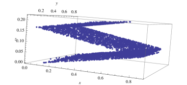
Figure 1: The chaotic attractor of map in Example 4.1 with $k_{1}=2.4$, $k_{2}=0.08,$ and $k_{3}=0.25$, where the initial value is taken as $(0.2,0.1,0.5)$.

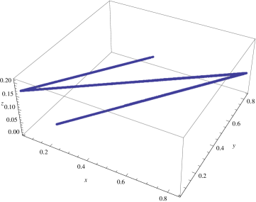
Figure 2: The chaotic attractor of map in Example 4.1 with $k_{1}=2.4$, $k_{2}=0.08,$ and $k_{3}=0.25$, where the initial value is taken as $(0.5,0.5,0.5)$.

References

• [1]
• [2] L. Barreira, Ya. Pesin, Lectures on Lyapunov Exponents and Smooth Ergodic Theory, Univ. Lect. Series. Vol 23, Amer. Math. Soc. 2002
• [3] M. Benedicks, L. Carleson, The dynamics of the HΓ©non map, Ann. Math.133 (1991), 73–169.
• [4] M. Benedicks, M. Viana, Solution of the basin problem for HΓ©non-like attractors, Invent. Math. 143 (2001), 375–434.
• [5] M. Benedicks, L. S. Young, Sinai-Bowen-Ruelle measure for certain HΓ©non maps, Invent. Math. 112 (1993), 541–576.
• [6] R. Bowen, Equilibrium states and the ergodic theory of Anosov diffeomorhisms, Lecture Notes in Math. 470, Springer, New York, 1975.
• [7] A. Boyarsky, P. GΓ³ra, Laws of Chaos. Invariant measures and Dynamical Systems in One Dimensions, Probability and its applications, BirkhaΓΌser., Boston, MA, 1997
• [8] N. Chernov, R. Markarian, Chaotic Billiards, Mathematical Surveys and Monographs, Vol. 127, Amer. Math. Soc. 2006.
• [9] P. Collet, Y. Levy, Ergodic Properties of the Lozi Mappings, Commun. Math. Phys. 93 (1984), 461–481.
• [10] L. C. Evans, R. F. Gariepy, Measure Theory and Fine Properties of Functions (Studies in Advanced Mathematics). CRC Press, Boca Raton, FL, 1992.
• [11] M. Jakobson, S. Newhouse, A two-dimensional version of the folklore theorem, Amer. Math. Soc. Transl. 2 (1996) 89–105.
• [12] A. Katok, J. M. Strelcyn, Invariant Manifolds, Entropy and Billiards, Smooth Maps with Singularities,with the collaboration of A. Ledrappier and F. Przytycki, Lect. Notes. Math. vol 1222, Springer-Verlag, Berlin, Heidelber, New York, London, Paris, Tokyo, 1986.
• [13] F. Ledrappier, PropriΓ©tΓ©s ergodiques des measure de Sinai. Publ. Math. IHES 59 (1984), 163–188.
• [14] A. Lasota, J. A. Yorke, On the existence of invariant measures for piecewise monotonic transformations, Trans. Amer. Math. Soc. 186 (1973) 481–488.
• [15] C. Liverani, Multidimensional expanding maps with singularities: a pedestrian approach, Ergod. Th. Dynam. Sys. 33 (2013), 168–182.
• [16] Ya. B. Pesin, Families of invariant manifolds corresponding to non-zero characteristics exponenets, Math. USSR-Izv. 10 (1978), 1261–1305.
• [17] F. SΓ‘nchez-Salas, Sinai-Ruelle-Bowen measures for piecewise hyperbolic transformations, Divulgaciones MatemΓ‘ticas 9 (2001), 35–54.
• [18] O. M. Sarig, Subexponential decay of corrlations, Invent. Math. 150 (2002) 629–653,
• [19] Ya. G. Sinai, Gibbs measures in ergodic theory, Russ. Math. Surveys 27, 4 (1972), 21–69.
• [20] Q. Wang, L. S. Young, Strange attractors with one direction of instability, Commun. Math. Phys. 218 (2001), 1–97.
• [21] L. S. Young, Bowen-Ruelle measures for certain piecewise hyperbolic maps, Trans. Amer Math. Soc. 287 (1985), 41–48.
• [22] L. S. Young, Statistical properties of dynamical systems with some hyperbolicity, Ann. Math. 147 (1998), 558–650.
• [23] L. S. Young, Recurrence times and rates of mixing, Isr. J. Math. 110 (1999), 153–188.
• [24] L. S. Young, What are SRB measures, and which dynamical systems have them? J. Statistical Physics, 108 (2002), 733–7554.