Abstract

Nuclear scissors modes are considered in the frame of Wigner function moments method generalized to take into account spin degrees of freedom and pair correlations simultaneously. A new source of nuclear magnetism, connected with counter-rotation of spins up and down around the symmetry axis (hidden angular momenta), is discovered. Its inclusion into the theory allows one to improve substantially the agreement with experimental data in the description of energies and transition probabilities of scissors modes in rare earth nuclei.

Keywords: spin, pairing, collective motion, scissors mode

PACS numbers: 21.10.Hw, 21.60.Ev, 21.60.Jz, 24.30.Cz

1 Introduction

The nuclear scissors mode was predicted [1]–[4] as a counter-rotation of protons against neutrons in deformed nuclei. However, its collectivity turned out to be small. From RPA results which were in qualitative agreement with experiment, it was even questioned whether this mode is collective at all [5, 6]. Purely phenomenological models (such as, e.g., the two rotors model [7]) and the sum rule approach [8] did not clear up the situation in this respect. Finally in a recent review [9] it is concluded that the scissors mode is ”weakly collective, but strong on the single-particle scale” and further: ”The weakly collective scissors mode excitation has become an ideal test of models – especially microscopic models – of nuclear vibrations. Most models are usually calibrated to reproduce properties of strongly collective excitations (e.g. of $J^{\pi}=2^{+}$ or $3^{-}$ states, giant resonances, …). Weakly-collective phenomena, however, force the models to make genuine predictions and the fact that the transitions in question are strong on the single-particle scale makes it impossible to dismiss failures as a mere detail, especially in the light of the overwhelming experimental evidence for them in many nuclei [10, 11].”

The Wigner Function Moments (WFM) or phase space moments method turns out to be very useful in this situation. On the one hand it is a purely microscopic method, because it is based on the Time Dependent Hartree-Fock (TDHF) equation. On the other hand the method works with average values (moments) of operators which have a direct relation to the considered phenomenon and, thus, make a natural bridge with the macroscopic description. This makes it an ideal instrument to describe the basic characteristics (energies and excitation probabilities) of collective excitations such as, in particular, the scissors mode.

Further developments of the WFM method, namely, the switch from TDHF to TDHF-Bogoliubov (TDHFB) equations, i.e. taking into account pair correlations, allowed us to improve considerably the quantitative description of the scissors mode [12, 13]: for rare earth nuclei the energies were reproduced with $\sim 10\%$ accuracy and B(M1) values were reduced by about a factor of two with respect to their non superfluid values. However, they remained about two times too high with respect to experiment. We have suspected, that the reason of this last discrepancy is hidden in the spin degrees of freedom, which were so far ignored by the WFM method.

In a recent paper [14] the WFM method was applied for the first time to solve the TDHF equations including spin dynamics. As a first step, only the spin orbit interaction was included in the consideration, as the most important one among all possible spin dependent interactions because it enters into the mean field. The most remarkable result was the discovery of a new type of nuclear collective motion: rotational oscillations of ”spin-up” nucleons with respect of ”spin-down” nucleons (the spin scissors mode). It turns out that the experimentally observed group of peaks in the energy interval 2-4 MeV corresponds very likely to two different types of motion: the orbital scissors mode and this new kind of mode, i.e. the spin scissors mode. The pictorial view of these two intermingled scissors is shown on Fig. 1, which is just the modification (or generalization) of the classical picture for the orbital scissors (see, for example, [7, 9]).

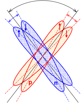
Figure 1: Pictorial representation of two intermingled scissors: the orbital (neutrons versus protons) scissors + spin (spin-up nucleons versus spin-down nucleons) scissors. Arrows inside of ellipses show the direction of spin projections. p - protons, n - neutrons.

The next step was done in the paper [15], where the influence of the spin-spin interaction on the scissors modes was studied. There was hope that, due to spin dependent interactions, some part of the force of M1 transitions will be shifted to the energy region of 5-10 MeV (the area of a spin-flip resonance), decreasing in such a way the M1 force of scissors. However, these expectations were not realised. It turned out that the spin-spin interaction does not change the general picture of the positions of excitations described in [14] pushing all levels up proportionally to its strength without changing their order. The most interesting result concerns the B(M1) values of both scissors – the spin-spin interaction strongly redistributes M1 strength in favour of the spin scissors mode practically without changing their summed strength.

In the present work we suggest a generalization of the WFM method which takes into account spin degrees of freedom and pair correlations simultaneously. According to our previous calculations these two factors, working together, should improve considerably the agreement between the theory and experiment in the description of nuclear scissors modes.

The paper is organized as follows. In Sec. 2 the TDHFB equations for the 2x2 normal and anomalous density matrices are formulated and their Wigner transform is found. In Sec. 3 the model Hamiltonian and the mean field are analyzed. In Sec. 4 the collective variables are defined and the respective dynamical equations are derived. In Sec. 5 the choice of parameters and the results of calculations of energies and B(M1) values of two scissors modes are discussed. The phenomenon of counter-rotating angular momenta with spin up/down, which can be considered also as a phenomenon of hidden angular momenta, is analysed in Sec. 6. Results of calculations for 26 nuclei in the rare earth region are discussed in Sec. 7. The summary of main results is given in the conclusion section. The mathematical details are concentrated in Appendices A, B, C, D.

2 Wigner transformation of TDHFB equations

The Time-Dependent Hartree–Fock–Bogoliubov (TDHFB) equations in matrix formulation are [16, 17]

$$i\hbar\dot{\cal R}=[{\cal H},{\cal R}]$$ (1)

with

$${\cal R}={\hat{\rho}\qquad-\hat{\kappa}\choose-\hat{\kappa}^{\dagger}\;\;1-\hat{\rho}^{*}},\quad{\cal H}={\hat{h}\quad\;\;\hat{\Delta}\choose\hat{\Delta}^{\dagger}\quad-\hat{h}^{*}}$$ (2)

The normal density matrix $\hat{\rho}$ and Hamiltonian $\hat{h}$ are hermitian whereas the abnormal density $\hat{\kappa}$ and the pairing gap $\hat{\Delta}$ are skew symmetric: $\hat{\kappa}^{\dagger}=-\hat{\kappa}^{*}$, $\hat{\Delta}^{\dagger}=-\hat{\Delta}^{*}$.

The detailed form of the TDHFB equations is

$$i\hbar\dot{\hat{\rho}}=\hat{h}\hat{\rho}-\hat{\rho}\hat{h}-\hat{\Delta}\hat{\kappa}^{\dagger}+\hat{\kappa}\hat{\Delta}^{\dagger},$$

$$-i\hbar\dot{\hat{\rho}}^{*}=\hat{h}^{*}\hat{\rho}^{*}-\hat{\rho}^{*}\hat{h}^{*}-\hat{\Delta}^{\dagger}\hat{\kappa}+\hat{\kappa}^{\dagger}\hat{\Delta},$$

$$-i\hbar\dot{\hat{\kappa}}=-\hat{h}\hat{\kappa}-\hat{\kappa}\hat{h}^{*}+\hat{\Delta}-\hat{\Delta}\hat{\rho}^{*}-\hat{\rho}\hat{\Delta},$$

$$-i\hbar\dot{\hat{\kappa}}^{\dagger}=\hat{h}^{*}\hat{\kappa}^{\dagger}+\hat{\kappa}^{\dagger}\hat{h}-\hat{\Delta}^{\dagger}+\hat{\Delta}^{\dagger}\hat{\rho}+\hat{\rho}^{*}\hat{\Delta}^{\dagger}.$$ (3)

It is easy to see that the second and fourth equations are complex conjugate to the first and third ones respectively. Let us consider their matrix form in coordinate space keeping all spin indices $s,s^{\prime},s^{\prime\prime}$:

$$i\hbar\langle{\bf r},s|\dot{\hat{\rho}}|{\bf r}^{\prime\prime},s^{\prime\prime}\rangle=\hskip 341.43306pt$$

$$\hskip 28.45274pt\sum_{s^{\prime}}\int\!d^{3}r^{\prime}\left(\langle{\bf r},s|\hat{h}|{\bf r}^{\prime},s^{\prime}\rangle\langle{\bf r}^{\prime},s^{\prime}|\hat{\rho}|{\bf r}^{\prime\prime},s^{\prime\prime}\rangle-\langle{\bf r},s|\hat{\rho}|{\bf r}^{\prime},s^{\prime}\rangle\langle{\bf r}^{\prime},s^{\prime}|\hat{h}|{\bf r}^{\prime\prime},s^{\prime\prime}\rangle\right.$$

$$\hskip 28.45274pt\left.-\langle{\bf r},s|\hat{\Delta}|{\bf r}^{\prime},s^{\prime}\rangle\langle{\bf r}^{\prime},s^{\prime}|\hat{\kappa}^{\dagger}|{\bf r}^{\prime\prime},s^{\prime\prime}\rangle+\langle{\bf r},s|\hat{\kappa}|{\bf r}^{\prime},s^{\prime}\rangle\langle{\bf r}^{\prime},s^{\prime}|\hat{\Delta}^{\dagger}|{\bf r}^{\prime\prime},s^{\prime\prime}\rangle\right),$$

$$i\hbar\langle{\bf r},s|\dot{\hat{\kappa}}|{\bf r}^{\prime\prime},s^{\prime\prime}\rangle=-\langle{\bf r},s|\hat{\Delta}|{\bf r}^{\prime\prime},s^{\prime\prime}\rangle\hskip 241.84842pt$$

$$\hskip 28.45274pt+\sum_{s^{\prime}}\int\!d^{3}r^{\prime}\left(\langle{\bf r},s|\hat{h}|{\bf r}^{\prime},s^{\prime}\rangle\langle{\bf r}^{\prime},s^{\prime}|\hat{\kappa}|{\bf r}^{\prime\prime},s^{\prime\prime}\rangle+\langle{\bf r},s|\hat{\kappa}|{\bf r}^{\prime},s^{\prime}\rangle\langle{\bf r}^{\prime},s^{\prime}|\hat{h}^{*}|{\bf r}^{\prime\prime},s^{\prime\prime}\rangle\right.$$

$$\hskip 28.45274pt\left.+\langle{\bf r},s|\hat{\Delta}|{\bf r}^{\prime},s^{\prime}\rangle\langle{\bf r}^{\prime},s^{\prime}|\hat{\rho}^{*}|{\bf r}^{\prime\prime},s^{\prime\prime}\rangle+\langle{\bf r},s|\hat{\rho}|{\bf r}^{\prime},s^{\prime}\rangle\langle{\bf r}^{\prime},s^{\prime}|\hat{\Delta}|{\bf r}^{\prime\prime},s^{\prime\prime}\rangle\right),$$

$$i\hbar\langle{\bf r},s|\dot{\hat{\rho}}^{*}|{\bf r}^{\prime\prime},s^{\prime\prime}\rangle=\hskip 341.43306pt$$

$$\hskip 28.45274pt\sum_{s^{\prime}}\int\!d^{3}r^{\prime}\left(-\langle{\bf r},s|\hat{h}^{*}|{\bf r}^{\prime},s^{\prime}\rangle\langle{\bf r}^{\prime},s^{\prime}|\hat{\rho}^{*}|{\bf r}^{\prime\prime},s^{\prime\prime}\rangle+\langle{\bf r},s|\hat{\rho}^{*}|{\bf r}^{\prime},s^{\prime}\rangle\langle{\bf r}^{\prime},s^{\prime}|\hat{h}^{*}|{\bf r}^{\prime\prime},s^{\prime\prime}\rangle\right.$$

$$\hskip 28.45274pt\left.+\langle{\bf r},s|\hat{\Delta}^{\dagger}|{\bf r}^{\prime},s^{\prime}\rangle\langle{\bf r}^{\prime},s^{\prime}|\hat{\kappa}|{\bf r}^{\prime\prime},s^{\prime\prime}\rangle-\langle{\bf r},s|\hat{\kappa}^{\dagger}|{\bf r}^{\prime},s^{\prime}\rangle\langle{\bf r}^{\prime},s^{\prime}|\hat{\Delta}|{\bf r}^{\prime\prime},s^{\prime\prime}\rangle\right),$$

$$i\hbar\langle{\bf r},s|\dot{\hat{\kappa}}^{\dagger}|{\bf r}^{\prime\prime},s^{\prime\prime}\rangle=\langle{\bf r},s|\hat{\Delta}^{\dagger}|{\bf r}^{\prime\prime},s^{\prime\prime}\rangle\hskip 241.84842pt$$

$$\hskip 28.45274pt+\sum_{s^{\prime}}\int\!d^{3}r^{\prime}\left(-\langle{\bf r},s|\hat{h}^{*}|{\bf r}^{\prime},s^{\prime}\rangle\langle{\bf r}^{\prime},s^{\prime}|\hat{\kappa}^{\dagger}|{\bf r}^{\prime\prime},s^{\prime\prime}\rangle-\langle{\bf r},s|\hat{\kappa}^{\dagger}|{\bf r}^{\prime},s^{\prime}\rangle\langle{\bf r}^{\prime},s^{\prime}|\hat{h}|{\bf r}^{\prime\prime},s^{\prime\prime}\rangle\right.$$

$$\hskip 28.45274pt\left.-\langle{\bf r},s|\hat{\Delta}^{\dagger}|{\bf r}^{\prime},s^{\prime}\rangle\langle{\bf r}^{\prime},s^{\prime}|\hat{\rho}|{\bf r}^{\prime\prime},s^{\prime\prime}\rangle-\langle{\bf r},s|\hat{\rho}^{*}|{\bf r}^{\prime},s^{\prime}\rangle\langle{\bf r}^{\prime},s^{\prime}|\hat{\Delta}^{\dagger}|{\bf r}^{\prime\prime},s^{\prime\prime}\rangle\right).$$ (4)

We do not specify the isospin indices in order to make formulae more transparent. They will be re-introduced at the end. Let us introduce the more compact notation $\langle{\bf r},s|\hat{X}|{\bf r}^{\prime},s^{\prime}\rangle=X_{rr^{\prime}}^{ss^{\prime}}$. Then the set of TDHFB equations (4) with specified spin indices reads

$$i\hbar\dot{\rho}_{rr^{\prime\prime}}^{\uparrow\uparrow}=\int\!d^{3}r^{\prime}(h_{rr^{\prime}}^{\uparrow\uparrow}\rho_{r^{\prime}r^{\prime\prime}}^{\uparrow\uparrow}-\rho_{rr^{\prime}}^{\uparrow\uparrow}h_{r^{\prime}r^{\prime\prime}}^{\uparrow\uparrow}+\hat{h}_{rr^{\prime}}^{\uparrow\downarrow}\rho_{r^{\prime}r^{\prime\prime}}^{\downarrow\uparrow}-\rho_{rr^{\prime}}^{\uparrow\downarrow}h_{r^{\prime}r^{\prime\prime}}^{\downarrow\uparrow}-\Delta_{rr^{\prime}}^{\uparrow\downarrow}{\kappa^{\dagger}}_{r^{\prime}r^{\prime\prime}}^{\downarrow\uparrow}+\kappa_{rr^{\prime}}^{\uparrow\downarrow}{\Delta^{\dagger}}_{r^{\prime}r^{\prime\prime}}^{\downarrow\uparrow}),$$

$$i\hbar\dot{\rho}_{rr^{\prime\prime}}^{\uparrow\downarrow}=\int\!d^{3}r^{\prime}(h_{rr^{\prime}}^{\uparrow\uparrow}\rho_{r^{\prime}r^{\prime\prime}}^{\uparrow\downarrow}-\rho_{rr^{\prime}}^{\uparrow\uparrow}h_{r^{\prime}r^{\prime\prime}}^{\uparrow\downarrow}+\hat{h}_{rr^{\prime}}^{\uparrow\downarrow}\rho_{r^{\prime}r^{\prime\prime}}^{\downarrow\downarrow}-\rho_{rr^{\prime}}^{\uparrow\downarrow}h_{r^{\prime}r^{\prime\prime}}^{\downarrow\downarrow}),$$

$$i\hbar\dot{\rho}_{rr^{\prime\prime}}^{\downarrow\uparrow}=\int\!d^{3}r^{\prime}(h_{rr^{\prime}}^{\downarrow\uparrow}\rho_{r^{\prime}r^{\prime\prime}}^{\uparrow\uparrow}-\rho_{rr^{\prime}}^{\downarrow\uparrow}h_{r^{\prime}r^{\prime\prime}}^{\uparrow\uparrow}+\hat{h}_{rr^{\prime}}^{\downarrow\downarrow}\rho_{r^{\prime}r^{\prime\prime}}^{\downarrow\uparrow}-\rho_{rr^{\prime}}^{\downarrow\downarrow}h_{r^{\prime}r^{\prime\prime}}^{\downarrow\uparrow}),$$

$$i\hbar\dot{\rho}_{rr^{\prime\prime}}^{\downarrow\downarrow}=\int\!d^{3}r^{\prime}(h_{rr^{\prime}}^{\downarrow\uparrow}\rho_{r^{\prime}r^{\prime\prime}}^{\uparrow\downarrow}-\rho_{rr^{\prime}}^{\downarrow\uparrow}h_{r^{\prime}r^{\prime\prime}}^{\uparrow\downarrow}+\hat{h}_{rr^{\prime}}^{\downarrow\downarrow}\rho_{r^{\prime}r^{\prime\prime}}^{\downarrow\downarrow}-\rho_{rr^{\prime}}^{\downarrow\downarrow}h_{r^{\prime}r^{\prime\prime}}^{\downarrow\downarrow}-\Delta_{rr^{\prime}}^{\downarrow\uparrow}{\kappa^{\dagger}}_{r^{\prime}r^{\prime\prime}}^{\uparrow\downarrow}+\kappa_{rr^{\prime}}^{\downarrow\uparrow}{\Delta^{\dagger}}_{r^{\prime}r^{\prime\prime}}^{\uparrow\downarrow}),$$

$$i\hbar\dot{\kappa}_{rr^{\prime\prime}}^{\uparrow\downarrow}=-\hat{\Delta}_{rr^{\prime\prime}}^{\uparrow\downarrow}+\int\!d^{3}r^{\prime}\left(h_{rr^{\prime}}^{\uparrow\uparrow}\kappa_{r^{\prime}r^{\prime\prime}}^{\uparrow\downarrow}+\kappa_{rr^{\prime}}^{\uparrow\downarrow}{h^{*}}_{r^{\prime}r^{\prime\prime}}^{\downarrow\downarrow}+\Delta_{rr^{\prime}}^{\uparrow\downarrow}{\rho^{*}}_{r^{\prime}r^{\prime\prime}}^{\downarrow\downarrow}+\rho_{rr^{\prime}}^{\uparrow\uparrow}\Delta_{r^{\prime}r^{\prime\prime}}^{\uparrow\downarrow}\right),$$

$$i\hbar\dot{\kappa}_{rr^{\prime\prime}}^{\downarrow\uparrow}=-\hat{\Delta}_{rr^{\prime\prime}}^{\downarrow\uparrow}+\int\!d^{3}r^{\prime}\left(h_{rr^{\prime}}^{\downarrow\downarrow}\kappa_{r^{\prime}r^{\prime\prime}}^{\downarrow\uparrow}+\kappa_{rr^{\prime}}^{\downarrow\uparrow}{h^{*}}_{r^{\prime}r^{\prime\prime}}^{\uparrow\uparrow}+\Delta_{rr^{\prime}}^{\downarrow\uparrow}{\rho^{*}}_{r^{\prime}r^{\prime\prime}}^{\uparrow\uparrow}+\rho_{rr^{\prime}}^{\downarrow\downarrow}\Delta_{r^{\prime}r^{\prime\prime}}^{\downarrow\uparrow}\right).$$ (5)

This set of equations must be complemented by the complex conjugated equations. Writing these equations, we neglected the diagonal matrix elements in spin, $\kappa_{rr^{\prime}}^{ss}$ and $\Delta_{rr^{\prime}}^{ss}$. It is shown in Appendix A that such approximation works very well in the case of monopole pairing considered here.

We will work with the Wigner transform [17] of equations (5). The relevant mathematical details can be found in [12]. The most essential relations are outlined in Appendix B. ¿From now on, we will not write out the coordinate dependence $({\bf r},{\bf p})$ of all functions in order to make the formulae more transparent. The Wigner transform of (5) can be written as

$$i\hbar\dot{f}^{\uparrow\uparrow} = i\hbar\{h^{\uparrow\uparrow},f^{\uparrow\uparrow}\}+h^{\uparrow\downarrow}f^{\downarrow\uparrow}-f^{\uparrow\downarrow}h^{\downarrow\uparrow}+\frac{i\hbar}{2}\{h^{\uparrow\downarrow},f^{\downarrow\uparrow}\}-\frac{i\hbar}{2}\{f^{\uparrow\downarrow},h^{\downarrow\uparrow}\}$$

$$- \frac{\hbar^{2}}{8}\{\!\{h^{\uparrow\downarrow},f^{\downarrow\uparrow}\}\!\}+\frac{\hbar^{2}}{8}\{\!\{f^{\uparrow\downarrow},h^{\downarrow\uparrow}\}\!\}+\kappa\Delta^{*}-\Delta\kappa^{*}$$

$$+ \frac{i\hbar}{2}\{\kappa,\Delta^{*}\}-\frac{i\hbar}{2}\{\Delta,\kappa^{*}\}-\frac{\hbar^{2}}{8}\{\!\{\kappa,\Delta^{*}\}\!\}+\frac{\hbar^{2}}{8}\{\!\{\Delta,\kappa^{*}\}\!\}+...,$$

$$i\hbar\dot{f}^{\downarrow\downarrow} = i\hbar\{h^{\downarrow\downarrow},f^{\downarrow\downarrow}\}+h^{\downarrow\uparrow}f^{\uparrow\downarrow}-f^{\downarrow\uparrow}h^{\uparrow\downarrow}+\frac{i\hbar}{2}\{h^{\downarrow\uparrow},f^{\uparrow\downarrow}\}-\frac{i\hbar}{2}\{f^{\downarrow\uparrow},h^{\uparrow\downarrow}\}$$

$$- \frac{\hbar^{2}}{8}\{\!\{h^{\downarrow\uparrow},f^{\uparrow\downarrow}\}\!\}+\frac{\hbar^{2}}{8}\{\!\{f^{\downarrow\uparrow},h^{\uparrow\downarrow}\}\!\}+\bar{\Delta}^{*}\bar{\kappa}-\bar{\kappa}^{*}\bar{\Delta}$$

$$+ \frac{i\hbar}{2}\{\bar{\Delta}^{*},\bar{\kappa}\}-\frac{i\hbar}{2}\{\bar{\kappa}^{*},\bar{\Delta}\}-\frac{\hbar^{2}}{8}\{\!\{\bar{\Delta}^{*},\bar{\kappa}\}\!\}+\frac{\hbar^{2}}{8}\{\!\{\bar{\kappa}^{*},\bar{\Delta}\}\!\}+...,$$

$$i\hbar\dot{f}^{\uparrow\downarrow} = f^{\uparrow\downarrow}(h^{\uparrow\uparrow}-h^{\downarrow\downarrow})+\frac{i\hbar}{2}\{(h^{\uparrow\uparrow}+h^{\downarrow\downarrow}),f^{\uparrow\downarrow}\}-\frac{\hbar^{2}}{8}\{\!\{(h^{\uparrow\uparrow}-h^{\downarrow\downarrow}),f^{\uparrow\downarrow}\}\!\}$$

$$- h^{\uparrow\downarrow}(f^{\uparrow\uparrow}-f^{\downarrow\downarrow})+\frac{i\hbar}{2}\{h^{\uparrow\downarrow},(f^{\uparrow\uparrow}+f^{\downarrow\downarrow})\}+\frac{\hbar^{2}}{8}\{\!\{h^{\uparrow\downarrow},(f^{\uparrow\uparrow}-f^{\downarrow\downarrow})\}\!\}+....,$$

$$i\hbar\dot{f}^{\downarrow\uparrow} = f^{\downarrow\uparrow}(h^{\downarrow\downarrow}-h^{\uparrow\uparrow})+\frac{i\hbar}{2}\{(h^{\downarrow\downarrow}+h^{\uparrow\uparrow}),f^{\downarrow\uparrow}\}-\frac{\hbar^{2}}{8}\{\!\{(h^{\downarrow\downarrow}-h^{\uparrow\uparrow}),f^{\downarrow\uparrow}\}\!\}$$

$$- h^{\downarrow\uparrow}(f^{\downarrow\downarrow}-f^{\uparrow\uparrow})+\frac{i\hbar}{2}\{h^{\downarrow\uparrow},(f^{\downarrow\downarrow}+f^{\uparrow\uparrow})\}+\frac{\hbar^{2}}{8}\{\!\{h^{\downarrow\uparrow},(f^{\downarrow\downarrow}-f^{\uparrow\uparrow})\}\!\}+...,$$

$$i\hbar\dot{\kappa} = \kappa\,(h^{\uparrow\uparrow}+\bar{h}^{\downarrow\downarrow})+\frac{i\hbar}{2}\{(h^{\uparrow\uparrow}-\bar{h}^{\downarrow\downarrow}),\kappa\}-\frac{\hbar^{2}}{8}\{\!\{(h^{\uparrow\uparrow}+\bar{h}^{\downarrow\downarrow}),\kappa\}\!\}$$

$$+ \Delta\,(f^{\uparrow\uparrow}+\bar{f}^{\downarrow\downarrow})+\frac{i\hbar}{2}\{(f^{\uparrow\uparrow}-\bar{f}^{\downarrow\downarrow}),\Delta\}-\frac{\hbar^{2}}{8}\{\!\{(f^{\uparrow\uparrow}+\bar{f}^{\downarrow\downarrow}),\Delta\}\!\}-\Delta+...,$$

$$i\hbar\dot{\kappa}^{*} = -\kappa^{*}(h^{\uparrow\uparrow}+\bar{h}^{\downarrow\downarrow})+\frac{i\hbar}{2}\{(h^{\uparrow\uparrow}-\bar{h}^{\downarrow\downarrow}),\kappa^{*}\}+\frac{\hbar^{2}}{8}\{\!\{(h^{\uparrow\uparrow}+\bar{h}^{\downarrow\downarrow}),\kappa^{*}\}\!\}$$ (6)

$$- \Delta^{*}(f^{\uparrow\uparrow}+\bar{f}^{\downarrow\downarrow})+\frac{i\hbar}{2}\{(f^{\uparrow\uparrow}-\bar{f}^{\downarrow\downarrow}),\Delta^{*}\}+\frac{\hbar^{2}}{8}\{\!\{(f^{\uparrow\uparrow}+\bar{f}^{\downarrow\downarrow}),\Delta^{*}\}\!\}+\Delta^{*}+...,$$

where the functions $h$, $f$, $\Delta$, and $\kappa$ are the Wigner transforms of $\hat{h}$, $\hat{\rho}$, $\hat{\Delta}$, and $\hat{\kappa}$, respectively, $\bar{f}({\bf r},{\bf p})=f({\bf r},-{\bf p})$, $\{f,g\}$ is the Poisson bracket of the functions $f({\bf r},{\bf p})$ and $g({\bf r},{\bf p})$ and $\{\{f,g\}\}$ is their double Poisson bracket; the dots stand for terms proportional to higher powers of $\hbar$. This set of equations must be complemented by the dynamical equations for $\bar{f}^{\uparrow\uparrow},\bar{f}^{\downarrow\downarrow},\bar{f}^{\uparrow\downarrow},\bar{f}^{\downarrow\uparrow},\bar{\kappa},\bar{\kappa}^{*}$. They are obtained by the change ${\bf p}\rightarrow-{\bf p}$ in arguments of functions and Poisson brackets. So, in reality we deal with the set of twelve equations. We introduced the notation $\kappa\equiv\kappa^{\uparrow\downarrow}$ and $\Delta\equiv\Delta^{\uparrow\downarrow}$. Symmetry properties of matrices $\hat{\kappa},\hat{\Delta}$ and the properties of their Wigner transforms (see Appendix B) allow one to replace the functions $\kappa^{\downarrow\uparrow}({\bf r},{\bf p})$ and $\Delta^{\downarrow\uparrow}({\bf r},{\bf p})$ by the functions $\bar{\kappa}^{\uparrow\downarrow}({\bf r},{\bf p})$ and $\bar{\Delta}^{\uparrow\downarrow}({\bf r},{\bf p})$.

Following the paper [14] we will write above equations in terms of spin-scalar

$$f^{+}=f^{\uparrow\uparrow}+f^{\downarrow\downarrow}$$

and spin-vector

$$f^{-}=f^{\uparrow\uparrow}-f^{\downarrow\downarrow}$$

functions. Furthermore, it is useful to rewrite the obtained equations in terms of even and odd functions $f_{e}=\frac{1}{2}(f+\bar{f})$ and $f_{o}=\frac{1}{2}(f-\bar{f})$ and real and imaginary parts of $\kappa$ and $\Delta$: $\kappa^{r}=\frac{1}{2}(\kappa+\kappa^{*}),\,\kappa^{i}=\frac{1}{2i}(\kappa-\kappa^{*}),\,\Delta^{r}=\frac{1}{2}(\Delta+\Delta^{*}),\,\Delta^{i}=\frac{1}{2i}(\Delta-\Delta^{*})$. We have

$$i\hbar\dot{f}^{+}_{e} = \frac{i\hbar}{2}\left[\{h^{+}_{o},f^{+}_{e}\}+\{h^{+}_{e},f^{+}_{o}\}+\{h^{-}_{o},f^{-}_{e}\}+\{h^{-}_{e},f^{-}_{o}\}\right]$$

$$+ {i\hbar}\left[\{h^{\uparrow\downarrow}_{o},f^{\downarrow\uparrow}_{e}\}+\{h^{\uparrow\downarrow}_{e},f^{\downarrow\uparrow}_{o}\}+\{h^{\downarrow\uparrow}_{o},f^{\uparrow\downarrow}_{e}\}+\{h^{\downarrow\uparrow}_{e},f^{\uparrow\downarrow}_{o}\}\right]$$

$$+ 4i\left([\kappa^{i}_{e}\Delta^{r}_{e}]-[\kappa^{r}_{e}\Delta^{i}_{e}]+[\kappa^{i}_{o}\Delta^{r}_{o}]-[\kappa^{r}_{o}\Delta^{i}_{o}]\right)+...,$$

$$i\hbar\dot{f}^{+}_{o} = \frac{i\hbar}{2}\left[\{h^{+}_{o},f^{+}_{o}\}+\{h^{+}_{e},f^{+}_{e}\}+\{h^{-}_{o},f^{-}_{o}\}+\{h^{-}_{e},f^{-}_{e}\}\right]$$

$$+ {i\hbar}\left[\{h^{\uparrow\downarrow}_{o},f^{\downarrow\uparrow}_{o}\}+\{h^{\uparrow\downarrow}_{e},f^{\downarrow\uparrow}_{e}\}+\{h^{\downarrow\uparrow}_{o},f^{\uparrow\downarrow}_{o}\}+\{h^{\downarrow\uparrow}_{e},f^{\uparrow\downarrow}_{e}\}\right]$$

$$+ 2i\hbar\left(\{\kappa^{r}_{e},\Delta^{r}_{e}\}+\{\kappa^{i}_{e},\Delta^{i}_{e}\}+\{\kappa^{r}_{o},\Delta^{r}_{o}\}+\{\kappa^{i}_{o},\Delta^{i}_{o}\}\right)+...,$$

$$i\hbar\dot{f}^{-}_{e} = 2(h^{\uparrow\downarrow}_{e}f^{\downarrow\uparrow}_{e}+h^{\uparrow\downarrow}_{o}f^{\downarrow\uparrow}_{o}-h^{\downarrow\uparrow}_{e}f^{\uparrow\downarrow}_{e}-h^{\downarrow\uparrow}_{o}f^{\uparrow\downarrow}_{o})$$

$$+ \frac{i\hbar}{2}\left[\{h^{+}_{o},f^{-}_{e}\}+\{h^{+}_{e},f^{-}_{o}\}+\{h^{-}_{o},f^{+}_{e}\}+\{h^{-}_{e},f^{+}_{o}\}\right]$$

$$+ 2i\hbar\left(\{\kappa^{r}_{e},\Delta^{r}_{o}\}+\{\kappa^{i}_{e},\Delta^{i}_{o}\}+\{\kappa^{r}_{o},\Delta^{r}_{e}\}+\{\kappa^{i}_{o},\Delta^{i}_{e}\}\right)$$

$$- \frac{\hbar^{2}}{4}\left[\{\!\{h^{\uparrow\downarrow}_{e},f^{\downarrow\uparrow}_{e}\}\!\}+\{\!\{h^{\uparrow\downarrow}_{o},f^{\downarrow\uparrow}_{o}\}\!\}-\{\!\{h^{\downarrow\uparrow}_{e},f^{\uparrow\downarrow}_{e}\}\!\}-\{\!\{h^{\downarrow\uparrow}_{o},f^{\uparrow\downarrow}_{o}\}\!\}\right]+...,$$

$$i\hbar\dot{f}^{-}_{o} = 2(h^{\uparrow\downarrow}_{e}f^{\downarrow\uparrow}_{o}+h^{\uparrow\downarrow}_{o}f^{\downarrow\uparrow}_{e}-h^{\downarrow\uparrow}_{e}f^{\uparrow\downarrow}_{o}-h^{\downarrow\uparrow}_{o}f^{\uparrow\downarrow}_{e})$$

$$+ 4i\left([\kappa^{i}_{e}\Delta^{r}_{o}]-[\kappa^{r}_{e}\Delta^{i}_{o}]+[\kappa^{i}_{o}\Delta^{r}_{e}]-[\kappa^{r}_{o}\Delta^{i}_{e}]\right)$$

$$+ \frac{i\hbar}{2}\left[\{h^{+}_{o},f^{-}_{o}\}+\{h^{+}_{e},f^{-}_{e}\}+\{h^{-}_{o},f^{+}_{o}\}+\{h^{-}_{e},f^{+}_{e}\}\right]$$

$$- \frac{\hbar^{2}}{4}\left[\{\!\{h^{\uparrow\downarrow}_{e},f^{\downarrow\uparrow}_{o}\}\!\}+\{\!\{h^{\uparrow\downarrow}_{o},f^{\downarrow\uparrow}_{e}\}\!\}-\{\!\{h^{\downarrow\uparrow}_{e},f^{\uparrow\downarrow}_{o}\}\!\}-\{\!\{h^{\downarrow\uparrow}_{o},f^{\uparrow\downarrow}_{e}\}\!\}\right]+...,$$

$$i\hbar\dot{f}^{\uparrow\downarrow}_{e} = \left[h^{-}_{e}f^{\uparrow\downarrow}_{e}+h^{-}_{o}f^{\uparrow\downarrow}_{o}-h^{\uparrow\downarrow}_{e}f^{-}_{e}-h^{\uparrow\downarrow}_{o}f^{-}_{o}\right]$$

$$+ \frac{i\hbar}{2}\left[\{h^{\uparrow\downarrow}_{e},f^{+}_{o}\}+\{h^{\uparrow\downarrow}_{o},f^{+}_{e}\}+\{h^{+}_{e},f^{\uparrow\downarrow}_{o}\}+\{h^{+}_{o},f^{\uparrow\downarrow}_{e}\}\right]$$

$$+ \frac{\hbar^{2}}{8}\left[\{\!\{h^{\uparrow\downarrow}_{e},f^{-}_{e}\}\!\}+\{\!\{h^{\uparrow\downarrow}_{o},f^{-}_{o}\}\!\}-\{\!\{h^{-}_{e},f^{\uparrow\downarrow}_{e}\}\!\}-\{\!\{h^{-}_{o},f^{\uparrow\downarrow}_{o}\}\!\}\right]+...,$$

$$i\hbar\dot{f}^{\downarrow\uparrow}_{e} = -\left[h^{-}_{e}f^{\downarrow\uparrow}_{e}+h^{-}_{o}f^{\downarrow\uparrow}_{o}-h^{\downarrow\uparrow}_{e}f^{-}_{e}-h^{\downarrow\uparrow}_{o}f^{-}_{o}\right]$$

$$+ \frac{i\hbar}{2}\left[\{h^{\downarrow\uparrow}_{e},f^{+}_{o}\}+\{h^{\downarrow\uparrow}_{o},f^{+}_{e}\}+\{h^{+}_{e},f^{\downarrow\uparrow}_{o}\}+\{h^{+}_{o},f^{\downarrow\uparrow}_{e}\}\right]$$

$$- \frac{\hbar^{2}}{8}\left[\{\!\{h^{\downarrow\uparrow}_{e},f^{-}_{e}\}\!\}+\{\!\{h^{\downarrow\uparrow}_{o},f^{-}_{o}\}\!\}-\{\!\{h^{-}_{e},f^{\downarrow\uparrow}_{e}\}\!\}-\{\!\{h^{-}_{o},f^{\downarrow\uparrow}_{o}\}\!\}\right]+...,$$

$$i\hbar\dot{f}^{\uparrow\downarrow}_{o} = \left[h^{-}_{e}f^{\uparrow\downarrow}_{o}+h^{-}_{o}f^{\uparrow\downarrow}_{e}-h^{\uparrow\downarrow}_{e}f^{-}_{o}-h^{\uparrow\downarrow}_{o}f^{-}_{e}\right]$$

$$+ \frac{i\hbar}{2}\left[\{h^{\uparrow\downarrow}_{e},f^{+}_{e}\}+\{h^{\uparrow\downarrow}_{o},f^{+}_{o}\}+\{h^{+}_{e},f^{\uparrow\downarrow}_{e}\}+\{h^{+}_{o},f^{\uparrow\downarrow}_{o}\}\right]$$

$$+ \frac{\hbar^{2}}{8}\left[\{\!\{h^{\uparrow\downarrow}_{e},f^{-}_{o}\}\!\}+\{\!\{h^{\uparrow\downarrow}_{o},f^{-}_{e}\}\!\}-\{\!\{h^{-}_{e},f^{\uparrow\downarrow}_{o}\}\!\}-\{\!\{h^{-}_{o},f^{\uparrow\downarrow}_{e}\}\!\}\right]+...,$$

$$i\hbar\dot{f}^{\downarrow\uparrow}_{o} = -\left[h^{-}_{e}f^{\downarrow\uparrow}_{o}+h^{-}_{o}f^{\downarrow\uparrow}_{e}-h^{\downarrow\uparrow}_{e}f^{-}_{o}-h^{\downarrow\uparrow}_{o}f^{-}_{e}\right]$$

$$+ \frac{i\hbar}{2}\left[\{h^{\downarrow\uparrow}_{e},f^{+}_{e}\}+\{h^{\downarrow\uparrow}_{o},f^{+}_{o}\}+\{h^{+}_{e},f^{\downarrow\uparrow}_{e}\}+\{h^{+}_{o},f^{\downarrow\uparrow}_{o}\}\right]$$

$$- \frac{\hbar^{2}}{8}\left[\{\!\{h^{\downarrow\uparrow}_{e},f^{-}_{o}\}\!\}+\{\!\{h^{\downarrow\uparrow}_{o},f^{-}_{e}\}\!\}-\{\!\{h^{-}_{e},f^{\downarrow\uparrow}_{o}\}\!\}-\{\!\{h^{-}_{o},f^{\downarrow\uparrow}_{e}\}\!\}\right]+...,$$

$$i\hbar\dot{\kappa}^{r}_{e} = i[h^{+}_{e}\,\kappa^{i}_{e}+h^{-}_{o}\,\kappa^{i}_{o}]+\frac{i\hbar}{2}\{h^{+}_{o},\kappa^{r}_{e}+h^{-}_{e},\kappa^{r}_{o}\}$$

$$+ i[f^{+}_{e}\,\Delta^{i}_{e}+f^{-}_{o}\,\Delta^{i}_{o}]+\frac{i\hbar}{2}\{f^{+}_{o},\Delta^{r}_{e}+f^{-}_{e},\Delta^{r}_{o}\}-i\Delta^{i}_{e}+...,$$

$$i\hbar\dot{\kappa}^{r}_{o} = i[h^{+}_{e}\,\kappa^{i}_{o}+h^{-}_{o}\,\kappa^{i}_{e}]+\frac{i\hbar}{2}\{h^{+}_{o},\kappa^{r}_{o}+h^{-}_{e},\kappa^{r}_{e}\}$$

$$+ i[f^{+}_{e}\,\Delta^{i}_{o}+f^{-}_{o}\,\Delta^{i}_{e}]+\frac{i\hbar}{2}\{f^{+}_{o},\Delta^{r}_{o}+f^{-}_{e},\Delta^{r}_{e}\}-i\Delta^{i}_{o}+...,$$

$$i\hbar\dot{\kappa}^{i}_{e} = -i[h^{+}_{e}\,\kappa^{r}_{e}+h^{-}_{o}\,\kappa^{r}_{o}]+\frac{i\hbar}{2}\{h^{+}_{o},\kappa^{i}_{e}+h^{-}_{e},\kappa^{i}_{o}\}$$

$$- i[f^{+}_{e}\,\Delta^{r}_{e}+f^{-}_{o}\,\Delta^{r}_{o}]+\frac{i\hbar}{2}\{f^{+}_{o},\Delta^{i}_{e}+f^{-}_{e},\Delta^{i}_{o}\}+i\Delta^{r}_{e}+...,$$

$$i\hbar\dot{\kappa}^{i}_{o} = -i[h^{+}_{e}\,\kappa^{r}_{o}+h^{-}_{o}\,\kappa^{r}_{e}]+\frac{i\hbar}{2}\{h^{+}_{o},\kappa^{i}_{o}+h^{-}_{e},\kappa^{i}_{e}\}$$ (7)

$$- i[f^{+}_{e}\,\Delta^{r}_{o}+f^{-}_{o}\,\Delta^{r}_{e}]+\frac{i\hbar}{2}\{f^{+}_{o},\Delta^{i}_{o}+f^{-}_{e},\Delta^{i}_{e}\}+i\Delta^{r}_{o}+...,$$

The following notation is introduced here: $h^{\pm}=h^{\uparrow\uparrow}\pm h^{\downarrow\downarrow},\quad[ab]=ab-\frac{\hbar^{2}}{8}\{\!\{a,b\}\!\},\quad[ab+cd+...]=[ab]+[cd]+...,\quad\{a,b+c,d+...\}=\{a,b\}+\{c,d\}+...$.

These twelve equations will be solved by the method of moments in a small amplitude approximation. To this end all functions $f({\bf r},{\bf p},t)$ and $\kappa({\bf r},{\bf p},t)$ are divided into equilibrium part and deviation (variation): $f({\bf r},{\bf p},t)=f({\bf r},{\bf p})_{eq}+\delta f({\bf r},{\bf p},t)$, $\kappa({\bf r},{\bf p},t)=\kappa({\bf r},{\bf p})_{eq}+\delta\kappa({\bf r},{\bf p},t)$. Then equations are linearized neglecting quadratic terms.

From general arguments one can expect that the phase of $\Delta$ (and of $\kappa$, since both are linked, according to equation (20)) is much more relevant than its magnitude, since the former determines the superfluid velocity. After linearization, the phase of $\Delta$ (and of $\kappa$) is expressed by $\delta\Delta^{i}$ (and $\delta\kappa^{i}$), while $\delta\Delta^{r}$ (and $\delta\kappa^{r}$) describes oscillations of the magnitude of $\Delta$ (and of $\kappa$). Let us therefore assume that

$$\delta\kappa^{r}({\bf r},{\bf p})\ll\delta\kappa^{i}({\bf r},{\bf p}).$$ (8)

This assumption was explicitly confirmed in [18] for the case of superfluid trapped fermionic atoms, where it was shown that $\delta\Delta^{r}$ is suppressed with respect to $\delta\Delta^{i}$ by one order of $\Delta/E_{\rm F}$, where $E_{\rm F}$ denotes the Fermi energy.

The assumption (8) allows one to neglect all terms containing the variations $\delta\kappa^{r}$ and $\delta\Delta^{r}$ in the equations (7) after their linearization. In this case the ”small” variations $\delta\kappa^{r}$ and $\delta\Delta^{r}$ will not affect the dynamics of the ”big” variations $\delta\kappa^{i}$ and $\delta\Delta^{i}$ . This means that the dynamical equations for the ”big” variations can be considered independently from that of the ”small” variations, and we will finally deal with a set of only ten equations.

3 Model Hamiltonian

The microscopic Hamiltonian of the model, harmonic oscillator with spin orbit potential plus separable quadrupole-quadrupole and spin-spin residual interactions is given by

$$H=\sum\limits_{i=1}^{A}\left[\frac{\hat{\bf p}_{i}^{2}}{2m}+\frac{1}{2}m\omega^{2}{\bf r}_{i}^{2}-\eta\hat{\bf l}_{i}\hat{\bf S}_{i}\right]+H_{qq}+H_{ss}$$ (9)

with

$$H_{qq}=\!\sum_{\mu=-2}^{2}(-1)^{\mu}\left\{\bar{\kappa}\sum\limits_{i}^{Z}\!\sum\limits_{j}^{N}+\frac{\kappa}{2}\left[\sum\limits_{i,j(i\neq j)}^{Z}+\sum\limits_{i,j(i\neq j)}^{N}\right]\right\}q_{2-\mu}({\bf r}_{i})q_{2\mu}({\bf r}_{j}),$$ (10)

$$H_{ss}=\!\sum_{\mu=-1}^{1}(-1)^{\mu}\left\{\bar{\chi}\sum\limits_{i}^{Z}\!\sum\limits_{j}^{N}+\frac{\chi}{2}\left[\sum\limits_{i,j(i\neq j)}^{Z}+\sum\limits_{i,j(i\neq j)}^{N}\right]\right\}\hat{S}_{-\mu}(i)\hat{S}_{\mu}(j)\,\delta({\bf r}_{i}-{\bf r}_{j}),$$ (11)

where $N$ and $Z$ are the numbers of neutrons and protons and $\hat{S}_{\mu}$ are spin matrices [19]:

$$\hat{S}_{1}=-\frac{\hbar}{\sqrt{2}}{0\quad 1\choose 0\quad 0},\quad\hat{S}_{0}=\frac{\hbar}{2}{1\quad\,0\choose 0\,-\!1},\quad\hat{S}_{-1}=\frac{\hbar}{\sqrt{2}}{0\quad 0\choose 1\quad 0}.$$ (12)

3.1 Mean Field

Let us analyze the mean field generated by this Hamiltonian.

3.1.1 Spin-orbit Potential

Written in cyclic coordinates, the spin orbit part of the Hamiltonian reads

$$\hat{h}_{ls}=-\eta\sum_{\mu=-1}^{1}(-)^{\mu}\hat{l}_{\mu}\hat{S}_{-\mu}=-\eta{\quad\hat{l}_{0}\frac{\hbar}{2}\quad\;\hat{l}_{-1}\frac{\hbar}{\sqrt{2}}\choose-\hat{l}_{1}\frac{\hbar}{\sqrt{2}}\;-\hat{l}_{0}\frac{\hbar}{2}},$$

where [19]

$$\hat{l}_{\mu}=-\hbar\sqrt{2}\sum_{\nu,\alpha}C_{1\nu,1\alpha}^{1\mu}r_{\nu}\nabla_{\alpha},$$ (13)

cyclic coordinates $r_{-1},r_{0},r_{1}$ are defined in [19], $C_{1\sigma,1\nu}^{\lambda\mu}$ is a Clebsch-Gordan coefficient and

$$\hat{l}_{1}=\hbar(r_{0}\nabla_{1}-r_{1}\nabla_{0})=-\frac{1}{\sqrt{2}}(\hat{l}_{x}+i\hat{l}_{y}),\quad\hat{l}_{0}=\hbar(r_{-1}\nabla_{1}-r_{1}\nabla_{-1})=\hat{l}_{z},$$

$$\hat{l}_{-1}=\hbar(r_{-1}\nabla_{0}-r_{0}\nabla_{-1})=\frac{1}{\sqrt{2}}(\hat{l}_{x}-i\hat{l}_{y}),$$

$$\hat{l}_{x}=-i\hbar(y\nabla_{z}-z\nabla_{y}),\quad\hat{l}_{y}=-i\hbar(z\nabla_{x}-x\nabla_{z}),\quad\hat{l}_{z}=-i\hbar(x\nabla_{y}-y\nabla_{x}).$$ (14)

Matrix elements of $\hat{h}_{ls}$ in coordinate space can be obviously written [14] as

$$\langle{\bf r}_{1},s_{1}|\hat{h}_{ls}|{\bf r}_{2},s_{2}\rangle = -\frac{\hbar}{2}\eta\left[\hat{l}_{0}({\bf r}_{1})(\delta_{s_{1}\uparrow}\delta_{s_{2}\uparrow}-\delta_{s_{1}\downarrow}\delta_{s_{2}\downarrow})\right.$$ (15)

$$+\left.\sqrt{2}\,\hat{l}_{-1}({\bf r}_{1})\delta_{s_{1}\uparrow}\delta_{s_{2}\downarrow}-\sqrt{2}\,\hat{l}_{1}({\bf r}_{1})\delta_{s_{1}\downarrow}\delta_{s_{2}\uparrow}\right]\delta({\bf r}_{1}-{\bf r}_{2}).$$

Their Wigner transform reads [14]:

$$h_{ls}^{s_{1}s_{2}}({\bf r},{\bf p}) = -\frac{\hbar}{2}\eta\left[l_{0}({\bf r},{\bf p})(\delta_{s_{1}\uparrow}\delta_{s_{2}\uparrow}-\delta_{s_{1}\downarrow}\delta_{s_{2}\downarrow})\right.$$ (16)

$$+\left.\sqrt{2}l_{-1}({\bf r},{\bf p})\delta_{s_{1}\uparrow}\delta_{s_{2}\downarrow}-\sqrt{2}l_{1}({\bf r},{\bf p})\delta_{s_{1}\downarrow}\delta_{s_{2}\uparrow}\right],$$

where $l_{\mu}=-i\sqrt{2}\sum_{\nu,\alpha}C_{1\nu,1\alpha}^{1\mu}r_{\nu}p_{\alpha}$.

3.1.2 Quadrupole-quadrupole interaction

The contribution of $H_{qq}$ to the mean field potential is easily found by replacing one of the $q_{2\mu}$ operators by the average value. We have

$$V^{\tau}_{qq}=\sqrt{6}\sum_{\mu}(-1)^{\mu}Z_{2-\mu}^{\tau+}q_{2\mu}.$$ (17)

Here

$$Z_{2\mu}^{n+}=\kappa R_{2\mu}^{n+}+\bar{\kappa}R_{2\mu}^{p+}\,,\quad Z_{2\mu}^{p+}=\kappa R_{2\mu}^{p+}+\bar{\kappa}R_{2\mu}^{n+},\quad R_{2\mu}^{\tau+}(t)=\frac{1}{\sqrt{6}}\int d({\bf p},{\bf r})q_{2\mu}({\bf r})f^{\tau+}({\bf r},{\bf p},t)$$ (18)

with $\int\!d({\bf p},{\bf r})\equiv(2\pi\hbar)^{-3}\int\!d^{3}p\,\int\!d^{3}r$ and $\tau$ being the isospin index.

3.1.3 Spin-spin interaction

The analogous expression for $H_{ss}$ is found in a standard way [15] with the following result for the Wigner transform of the proton mean field:

$$V_{p}^{ss^{\prime}}({\bf r},t) = 3\chi\frac{\hbar^{2}}{8}\left[\delta_{s\downarrow}\delta_{s^{\prime}\uparrow}n_{p}^{\downarrow\uparrow}+\delta_{s\uparrow}\delta_{s^{\prime}\downarrow}n_{p}^{\uparrow\downarrow}-\delta_{s\downarrow}\delta_{s^{\prime}\downarrow}n_{p}^{\uparrow\uparrow}-\delta_{s\uparrow}\delta_{s^{\prime}\uparrow}n_{p}^{\downarrow\downarrow}\right]$$ (19)

$$+ \bar{\chi}\frac{\hbar^{2}}{8}\left[2\delta_{s\downarrow}\delta_{s^{\prime}\uparrow}n_{n}^{\downarrow\uparrow}+2\delta_{s\uparrow}\delta_{s^{\prime}\downarrow}n_{n}^{\uparrow\downarrow}+(\delta_{s\uparrow}\delta_{s^{\prime}\uparrow}-\delta_{s\downarrow}\delta_{s^{\prime}\downarrow})(n_{n}^{\uparrow\uparrow}-n_{n}^{\downarrow\downarrow})\right],$$

where ${\displaystyle n_{\tau}^{ss^{\prime}}({\bf r},t)=\int\frac{d^{3}p}{(2\pi\hbar)^{3}}f^{ss^{\prime}}_{\tau}({\bf r},{\bf p},t)}$. The Wigner transform of the neutron mean field $V_{n}^{ss^{\prime}}$ is obtained from (19) by the obvious change of indices $p\leftrightarrow n$.

3.2 Pair potential

The Wigner transform of the pair potential (pairing gap) $\Delta({\bf r},{\bf p})$ is related to the Wigner transform of the anomalous density by [17]

$$\Delta({\bf r},{\bf p})=-\int\!\frac{d^{3}p^{\prime}}{(2\pi\hbar)^{3}}v(|{\bf p}-{\bf p}^{\prime}|)\kappa({\bf r},{\bf p}^{\prime}),$$ (20)

where $v(p)$ is a Fourier transform of the two-body interaction. We take for the pairing interaction a simple Gaussian of strength $V_{0}$ and range $r_{p}$ [17]

$$v(p)=\beta e^{-\alpha p^{2}}\!,$$ (21)

with $\beta=-|V_{0}|(r_{p}\sqrt{\pi})^{3}$ and $\alpha=r_{p}^{2}/4\hbar^{2}$. For the values of the parameters, see section 5.1.

4 Equations of motion

Integrating the set of equations (7) over phase space with the weights

$$W=\{r\otimes p\}_{\lambda\mu},\,\{r\otimes r\}_{\lambda\mu},\,\{p\otimes p\}_{\lambda\mu},\mbox{ and }1$$ (22)

one gets dynamic equations for the following collective variables:

$${\cal L}^{\tau\varsigma}_{\lambda\mu}(t)=\int\!d({\bf p},{\bf r})\{r\otimes p\}_{\lambda\mu}\delta f^{\tau\varsigma}_{o}({\bf r},{\bf p},t),\quad{\cal R}^{\tau\varsigma}_{\lambda\mu}(t)=\int\!d({\bf p},{\bf r})\{r\otimes r\}_{\lambda\mu}\delta f^{\tau\varsigma}_{e}({\bf r},{\bf p},t),\quad$$

$${\cal P}^{\tau\varsigma}_{\lambda\mu}(t)=\int\!d({\bf p},{\bf r})\{p\otimes p\}_{\lambda\mu}\delta f^{\tau\varsigma}_{e}({\bf r},{\bf p},t),\quad{\cal F}^{\tau\varsigma}(t)=\int\!d({\bf p},{\bf r})\delta f^{\tau\varsigma}_{e}({\bf r},{\bf p},t),\quad$$

$$\tilde{{\cal L}}^{\tau}_{\lambda\mu}(t)=\int\!d({\bf p},{\bf r})\{r\otimes p\}_{\lambda\mu}\delta\kappa^{\tau i}_{o}({\bf r},{\bf p},t),\quad\tilde{{\cal R}}^{\tau}_{\lambda\mu}(t)=\int\!d({\bf p},{\bf r})\{r\otimes r\}_{\lambda\mu}\delta\kappa^{\tau i}_{e}({\bf r},{\bf p},t),\quad$$

$$\tilde{{\cal P}}^{\tau}_{\lambda\mu}(t)=\int\!d({\bf p},{\bf r})\{p\otimes p\}_{\lambda\mu}\delta\kappa^{\tau i}_{e}({\bf r},{\bf p},t),\quad$$ (23)

where $\varsigma\!=+,\,-,\,\uparrow\downarrow,\,\downarrow\uparrow,$ and $\displaystyle\quad\{r\otimes r\}_{\lambda\mu}=\sum\limits_{\sigma,\nu}C_{1\sigma,1\nu}^{\lambda\mu}r_{\sigma}r_{\nu}.$

The required expressions for $h^{\pm}$, $h^{\uparrow\downarrow}$ and $h^{\downarrow\uparrow}$ are

$$h_{\tau}^{+}=\frac{p^{2}}{m}+m\,\omega^{2}r^{2}+12\sum_{\mu}(-1)^{\mu}Z_{2\mu}^{\tau+}(t)\{r\otimes r\}_{2-\mu}+V_{\tau}^{+}({\bf r},t)-\mu^{\tau},$$

$\mu^{\tau}$ being the chemical potential of protons ($\tau=p$) or neutrons ($\tau=n$),

$$h_{\tau}^{-}=-\hbar\eta l_{0}+V_{\tau}^{-}({\bf r},t),\quad h_{\tau}^{\uparrow\downarrow}=-\frac{\hbar}{\sqrt{2}}\eta l_{-1}+V_{\tau}^{\uparrow\downarrow}({\bf r},t),\quad h_{\tau}^{\downarrow\uparrow}=\frac{\hbar}{\sqrt{2}}\eta l_{1}+V_{\tau}^{\downarrow\uparrow}({\bf r},t),$$

where according to (19)

$$V_{p}^{+}({\bf r},t)=-3\frac{\hbar^{2}}{8}\chi n_{p}^{+}({\bf r},t),\quad V_{p}^{-}({\bf r},t)=3\frac{\hbar^{2}}{8}\chi n_{p}^{-}({\bf r},t)+\frac{\hbar^{2}}{4}\bar{\chi}n_{n}^{-}({\bf r},t),$$

$$V_{p}^{\uparrow\downarrow}({\bf r},t)=3\frac{\hbar^{2}}{8}\chi n_{p}^{\uparrow\downarrow}({\bf r},t)+\frac{\hbar^{2}}{4}\bar{\chi}n_{n}^{\uparrow\downarrow}({\bf r},t),\quad V_{p}^{\downarrow\uparrow}({\bf r},t)=3\frac{\hbar^{2}}{8}\chi n_{p}^{\downarrow\uparrow}({\bf r},t)+\frac{\hbar^{2}}{4}\bar{\chi}n_{n}^{\downarrow\uparrow}({\bf r},t)$$ (24)

and the neutron potentials $V_{n}^{\varsigma}$ are obtained by the obvious change of indices $p\leftrightarrow n$. Variations of these mean fields read:

$$\delta h_{\tau}^{+}=12\sum_{\mu}(-1)^{\mu}\delta Z_{2\mu}^{\tau+}(t)\{r\otimes r\}_{2-\mu}+\delta V_{\tau}^{+}({\bf r},t),$$

where $\quad\delta Z_{2\mu}^{p+}=\kappa\delta R_{2\mu}^{p+}+\bar{\kappa}\delta R_{2\mu}^{n+},\quad\delta R_{\lambda\mu}^{\tau+}(t)\equiv{\cal R}_{\lambda\mu}^{\tau+}(t)\quad$ and

$$\delta V_{p}^{+}({\bf r},t)=-3\frac{\hbar^{2}}{8}\chi\delta n_{p}^{+}({\bf r},t),\quad{\displaystyle\delta n_{p}^{+}({\bf r},t)=\int\frac{d^{3}p}{(2\pi\hbar)^{3}}\delta f^{+}_{p}({\bf r},{\bf p},t)}.$$

Variations of $h^{-}$, $h^{\uparrow\downarrow}$ and $h^{\downarrow\uparrow}$ are obtained in a similar way. Variation of the pair potential is

$$\delta\Delta({\bf r},{\bf p},t)=-\int\!\frac{d^{3}p^{\prime}}{(2\pi\hbar)^{3}}v(|{\bf p}-{\bf p}^{\prime}|)\delta\kappa({\bf r},{\bf p}^{\prime},t).$$ (25)

We are interested in the scissors mode with quantum number $K^{\pi}=1^{+}$. Therefore, we only need the part of dynamic equations with $\mu=1$.

It is convenient to rewrite the dynamical equations in terms of isoscalar and isovector variables

$$\bar{\cal R}_{\lambda\mu}={\cal R}_{\lambda\mu}^{n}+{\cal R}_{\lambda\mu}^{p},\quad\bar{\cal P}_{\lambda\mu}={\cal P}_{\lambda\mu}^{n}+{\cal P}_{\lambda\mu}^{p},\quad\bar{\cal L}_{\lambda\mu}={\cal L}_{\lambda\mu}^{n}+{\cal L}_{\lambda\mu}^{p}.$$

$${\cal R}_{\lambda\mu}={\cal R}_{\lambda\mu}^{n}-{\cal R}_{\lambda\mu}^{p},\quad{\cal P}_{\lambda\mu}={\cal P}_{\lambda\mu}^{n}-{\cal P}_{\lambda\mu}^{p},\quad{\cal L}_{\lambda\mu}={\cal L}_{\lambda\mu}^{n}-{\cal L}_{\lambda\mu}^{p},$$ (26)

It also is natural to define isovector and isoscalar strength constants $\kappa_{1}=\frac{1}{2}(\kappa-\bar{\kappa})$ and $\kappa_{0}=\frac{1}{2}(\kappa+\bar{\kappa})$ connected by the relation $\kappa_{1}=\alpha\kappa_{0}$ [20]. Then the equations for the neutron and proton systems are transformed into isovector and isoscalar ones. Supposing that all equilibrium characteristics of the proton system are equal to that of the neutron system one decouples isovector and isoscalar equations. This approximations looks rather crude, nevertheless the possible corrections to it are very small, being of the order $(\frac{N-Z}{A})^{2}$. The integration yields the following set of equations for isovector variables:

$$\dot{{\cal L}}^{+}_{21} = \frac{1}{m}{\cal P}_{21}^{+}-\left[m\,\omega^{2}-4\sqrt{3}\alpha\kappa_{0}R_{00}^{\rm eq}+\sqrt{6}(1+\alpha)\kappa_{0}R_{20}^{\rm eq}\right]{\cal R}^{+}_{21}-i\hbar\frac{\eta}{2}\left[{\cal L}_{21}^{-}+2{\cal L}^{\uparrow\downarrow}_{22}+\sqrt{6}{\cal L}^{\downarrow\uparrow}_{20}\right],$$

$$\dot{{\cal L}}^{-}_{21} = \frac{1}{m}{\cal P}_{21}^{-}-\left[m\,\omega^{2}+\sqrt{6}\kappa_{0}R_{20}^{\rm eq}-\frac{\sqrt{3}}{20}\hbar^{2}\left(\chi-\frac{\bar{\chi}}{3}\right)\left(\frac{I_{1}}{a_{0}^{2}}+\frac{I_{1}}{a_{1}^{2}}\right)\left(\frac{a_{1}^{2}}{{\cal A}_{2}}-\frac{a_{0}^{2}}{{\cal A}_{1}}\right)\right]{\cal R}^{-}_{21}-i\hbar\frac{\eta}{2}{\cal L}_{21}^{+}$$

$$+\frac{4}{\hbar}|V_{0}|I_{rp}^{\kappa\Delta}(r^{\prime}){\tilde{\cal L}}_{21},$$

$$\dot{{\cal L}}^{\uparrow\downarrow}_{22} = \frac{1}{m}{\cal P}_{22}^{\uparrow\downarrow}-\left[m\,\omega^{2}-2\sqrt{6}\kappa_{0}R_{20}^{\rm eq}-\frac{\sqrt{3}}{5}\hbar^{2}\left(\chi-\frac{\bar{\chi}}{3}\right)\frac{I_{1}}{{\cal A}_{2}}\right]{\cal R}^{\uparrow\downarrow}_{22}-i\hbar\frac{\eta}{2}{\cal L}_{21}^{+},$$

$$\dot{{\cal L}}^{\downarrow\uparrow}_{20} = \frac{1}{m}{\cal P}_{20}^{\downarrow\uparrow}-\left[m\,\omega^{2}+2\sqrt{6}\kappa_{0}R_{20}^{\rm eq}\right]{\cal R}^{\downarrow\uparrow}_{20}+\frac{2}{\sqrt{3}}\kappa_{0}R_{20}^{\rm eq}\,{\cal R}^{\downarrow\uparrow}_{00}-i\hbar\frac{\eta}{2}\sqrt{\frac{3}{2}}{\cal L}_{21}^{+}$$

$$+\frac{\sqrt{3}}{15}\hbar^{2}\left(\chi-\frac{\bar{\chi}}{3}\right)I_{1}\,\left[\left(\frac{1}{{\cal A}_{2}}-\frac{2}{{\cal A}_{1}}\right){\cal R}_{20}^{\downarrow\uparrow}+\sqrt{2}\left(\frac{1}{{\cal A}_{2}}+\frac{1}{{\cal A}_{1}}\right){\cal R}_{00}^{\downarrow\uparrow}\right],$$

$$\dot{{\cal L}}^{+}_{11} = -3\sqrt{6}(1-\alpha)\kappa_{0}R_{20}^{\rm eq}\,{\cal R}^{+}_{21}-i\hbar\frac{\eta}{2}\left[{\cal L}_{11}^{-}+\sqrt{2}{\cal L}^{\downarrow\uparrow}_{10}\right],$$

$$\dot{{\cal L}}^{-}_{11} = -\left[3\sqrt{6}\kappa_{0}R_{20}^{\rm eq}-\frac{\sqrt{3}}{20}\hbar^{2}\left(\chi-\frac{\bar{\chi}}{3}\right)\left(\frac{I_{1}}{a_{0}^{2}}-\frac{I_{1}}{a_{1}^{2}}\right)\left(\frac{a_{1}^{2}}{{\cal A}_{2}}-\frac{a_{0}^{2}}{{\cal A}_{1}}\right)\right]{\cal R}^{-}_{21}-\hbar\frac{\eta}{2}\left[i{\cal L}_{11}^{+}+\hbar F^{\downarrow\uparrow}\right]$$

$$+\frac{4}{\hbar}|V_{0}|I_{rp}^{\kappa\Delta}(r^{\prime}){\tilde{\cal L}}_{11},$$

$$\dot{{\cal L}}^{\downarrow\uparrow}_{10} = -\hbar\frac{\eta}{2\sqrt{2}}\left[i{\cal L}_{11}^{+}+\hbar F^{\downarrow\uparrow}\right],$$

$$\dot{F}^{\downarrow\uparrow} = -\eta\left[{\cal L}_{11}^{-}+\sqrt{2}{\cal L}^{\downarrow\uparrow}_{10}\right],$$

$$\dot{{\cal R}}^{+}_{21} = \frac{2}{m}{\cal L}_{21}^{+}-i\hbar\frac{\eta}{2}\left[{\cal R}_{21}^{-}+2{\cal R}^{\uparrow\downarrow}_{22}+\sqrt{6}{\cal R}^{\downarrow\uparrow}_{20}\right],$$

$$\dot{{\cal R}}^{-}_{21} = \frac{2}{m}{\cal L}_{21}^{-}-i\hbar\frac{\eta}{2}{\cal R}_{21}^{+},$$

$$\dot{{\cal R}}^{\uparrow\downarrow}_{22} = \frac{2}{m}{\cal L}_{22}^{\uparrow\downarrow}-i\hbar\frac{\eta}{2}{\cal R}_{21}^{+},$$

$$\dot{{\cal R}}^{\downarrow\uparrow}_{20} = \frac{2}{m}{\cal L}_{20}^{\downarrow\uparrow}-i\hbar\frac{\eta}{2}\sqrt{\frac{3}{2}}{\cal R}_{21}^{+},$$

$$\dot{{\cal P}}^{+}_{21} = -2\left[m\,\omega^{2}+\sqrt{6}\kappa_{0}R_{20}^{\rm eq}\right]{\cal L}^{+}_{21}+6\sqrt{6}\kappa_{0}R_{20}^{\rm eq}{\cal L}^{+}_{11}-i\hbar\frac{\eta}{2}\left[{\cal P}_{21}^{-}+2{\cal P}^{\uparrow\downarrow}_{22}+\sqrt{6}{\cal P}^{\downarrow\uparrow}_{20}\right]$$

$$+\frac{3\sqrt{3}}{4}\hbar^{2}\chi\frac{I_{2}}{{\cal A}_{1}{\cal A}_{2}}\left[\left({\cal A}_{1}-{\cal A}_{2}\right){\cal L}_{21}^{+}+\left({\cal A}_{1}+{\cal A}_{2}\right){\cal L}_{11}^{+}\right]$$

$$+\frac{4}{\hbar}|V_{0}|I_{pp}^{\kappa\Delta}(r^{\prime}){\tilde{\cal P}}_{21},$$

$$\dot{{\cal P}}^{-}_{21} = -2\left[m\,\omega^{2}+\sqrt{6}\kappa_{0}R_{20}^{\rm eq}\right]{\cal L}^{-}_{21}+6\sqrt{6}\kappa_{0}R_{20}^{\rm eq}{\cal L}^{-}_{11}-6\sqrt{2}\kappa_{0}L_{10}^{-}(\rm eq){\cal R}^{+}_{21}-i\hbar\frac{\eta}{2}{\cal P}_{21}^{+}$$

$$+\frac{3\sqrt{3}}{4}\hbar^{2}\chi\frac{I_{2}}{{\cal A}_{1}{\cal A}_{2}}\left[\left({\cal A}_{1}-{\cal A}_{2}\right){\cal L}_{21}^{-}+\left({\cal A}_{1}+{\cal A}_{2}\right){\cal L}_{11}^{-}\right],$$

$$\dot{{\cal P}}^{\uparrow\downarrow}_{22} = -\left[2m\,\omega^{2}-4\sqrt{6}\kappa_{0}R_{20}^{\rm eq}-\frac{3\sqrt{3}}{2}\hbar^{2}\chi\frac{I_{2}}{{\cal A}_{2}}\right]{\cal L}^{\uparrow\downarrow}_{22}-i\hbar\frac{\eta}{2}{\cal P}_{21}^{+},$$

$$\dot{{\cal P}}^{\downarrow\uparrow}_{20} = -\left[2m\,\omega^{2}+4\sqrt{6}\kappa_{0}R_{20}^{\rm eq}\right]{\cal L}^{\downarrow\uparrow}_{20}+8\sqrt{3}\kappa_{0}R_{20}^{\rm eq}{\cal L}^{\downarrow\uparrow}_{00}-i\hbar\frac{\eta}{2}\sqrt{\frac{3}{2}}{\cal P}_{21}^{+}$$

$$+\frac{\sqrt{3}}{2}\hbar^{2}\chi\frac{I_{2}}{{\cal A}_{1}{\cal A}_{2}}\left[\left({\cal A}_{1}-2{\cal A}_{2}\right){\cal L}_{20}^{\downarrow\uparrow}+\sqrt{2}\left({\cal A}_{1}+{\cal A}_{2}\right){\cal L}_{00}^{\downarrow\uparrow}\right],$$

$$\dot{{\cal L}}^{\downarrow\uparrow}_{00} = \frac{1}{m}{\cal P}_{00}^{\downarrow\uparrow}-m\,\omega^{2}{\cal R}^{\downarrow\uparrow}_{00}+4\sqrt{3}\kappa_{0}R_{20}^{\rm eq}\,{\cal R}^{\downarrow\uparrow}_{20}$$

$$+\frac{1}{2\sqrt{3}}\hbar^{2}\left[\left(\chi-\frac{\bar{\chi}}{3}\right)I_{1}-\frac{9}{4}\chi I_{2}\right]\left[\left(\frac{2}{{\cal A}_{2}}-\frac{1}{{\cal A}_{1}}\right){\cal R}_{00}^{\downarrow\uparrow}+\sqrt{2}\left(\frac{1}{{\cal A}_{2}}+\frac{1}{{\cal A}_{1}}\right){\cal R}_{20}^{\downarrow\uparrow}\right],$$

$$\dot{{\cal R}}^{\downarrow\uparrow}_{00} = \frac{2}{m}{\cal L}_{00}^{\downarrow\uparrow},$$

$$\dot{{\cal P}}^{\downarrow\uparrow}_{00} = -2m\,\omega^{2}{\cal L}^{\downarrow\uparrow}_{00}+8\sqrt{3}\kappa_{0}R_{20}^{\rm eq}\,{\cal L}^{\downarrow\uparrow}_{20}+\frac{\sqrt{3}}{2}\hbar^{2}\chi I_{2}\left[\left(\frac{2}{{\cal A}_{2}}-\frac{1}{{\cal A}_{1}}\right){\cal L}_{00}^{\downarrow\uparrow}+\sqrt{2}\left(\frac{1}{{\cal A}_{2}}+\frac{1}{{\cal A}_{1}}\right){\cal L}_{20}^{\downarrow\uparrow}\right],$$

$$\dot{{\tilde{\cal R}}}_{21} = -\frac{1}{\hbar}\left(\frac{16}{5}\alpha\kappa_{0}{\cal K}_{4}+\Delta_{0}(r^{\prime})-\frac{3}{8}\hbar^{2}\chi\kappa_{0}(r^{\prime})\right){\cal R}^{+}_{21},$$

$$\dot{{\tilde{\cal P}}}_{21} = -\frac{1}{\hbar}\Delta_{0}(r^{\prime}){\cal P}^{+}_{21}+6\hbar\alpha\kappa_{0}{\cal K}_{0}{\cal R}^{+}_{21},$$

$$\dot{{\tilde{\cal L}}}_{21} = -\frac{1}{\hbar}\Delta_{0}(r^{\prime}){{\cal L}}^{-}_{21},$$

$$\dot{{\tilde{\cal L}}}_{11} = -\frac{1}{\hbar}\Delta_{0}(r^{\prime}){\cal L}^{-}_{11},$$ (27)

where ${\cal A}_{1}=\sqrt{2}\,R_{20}^{\rm eq}-R_{00}^{\rm eq}=\frac{Q_{00}}{\sqrt{3}}\left(1+\frac{4}{3}\delta\right),\quad{\cal A}_{2}=R_{20}^{\rm eq}/\sqrt{2}+R_{00}^{\rm eq}=-\frac{Q_{00}}{\sqrt{3}}\left(1-\frac{2}{3}\delta\right)$, $\quad\displaystyle a_{-1}=a_{1}=R_{0}\left(\frac{1-(2/3)\delta}{1+(4/3)\delta}\right)^{1/6}$ and $\displaystyle a_{0}=R_{0}\left(\frac{1-(2/3)\delta}{1+(4/3)\delta}\right)^{-1/3}$ are semiaxes of ellipsoid by which the shape of nucleus is approximated, $\delta$ – deformation parameter, $R_{0}=1.2A^{1/3}$ fm.

$$I_{1}=\frac{\pi}{4}\int\limits_{0}^{\infty}dr\,r^{4}\left(\frac{\partial n^{+}(r)}{\partial r}\right)^{2},\ I_{2}=\frac{\pi}{4}\int\limits_{0}^{\infty}dr\,r^{2}n^{+}(r)^{2},\quad n^{+}(r)=n_{p}^{+}+n_{n}^{+}=\frac{n_{0}}{1+{\rm e}^{\frac{r-R_{0}}{a}}}.$$

${\cal K}_{0}=\int d({\bf r},{\bf p})\kappa_{0}({\bf r},{\bf p}),\,{\cal K}_{4}=\int d({\bf r},{\bf p})r^{4}\kappa_{0}({\bf r},{\bf p})$. The functions $\kappa_{0}(r^{\prime})$, $\Delta_{0}(r^{\prime})$, $I_{rp}^{\kappa\Delta}(r^{\prime})$ and $I_{pp}^{\kappa\Delta}(r^{\prime})$ are discussed in the next section and are demonstrated in Appendix D. Deriving these equations we neglected double Poisson brackets containing $\kappa$ or $\Delta$, which are the quantum corrections to pair correlations. The isoscalar set of equations is easily obtained from (4) by taking $\alpha=1$, replacing $\bar{\chi}\to-\bar{\chi}$ and putting the marks ”bar” above all variables.

5 Results of calculations

The set of equations (4) coincides with the set of equations (27) of the paper [15] in the limit of zero pairing, i.e. if to omit the last four equations and to neglect the contributions from pairing in the dynamical equations for the variables ${{\cal L}}^{-}_{21},\,{{\cal L}}^{-}_{11},$ and ${{\cal P}}^{+}_{21}$ . On the other hand, the dynamical equations for ${\tilde{\cal P}}_{21}$ and ${\tilde{\cal R}}_{21}$ and the contribution from pairing in the dynamical equation for ${{\cal P}}_{21}^{+}$ are exactly the same as the ones in the paper [13]. Only the dynamical equations for ${\tilde{\cal L}}_{21},\,$ ${\tilde{\cal L}}_{11}$ and the contributions from pairing in dynamical equations for ${{\cal L}}^{-}_{21},\,$ ${{\cal L}}^{-}_{11}$ are completely new.

Imposing the time evolution via $\displaystyle{e^{iEt/\hbar}}$ for all variables one transforms (4) into a set of algebraic equations. It contains 23 equations. To find the eigenvalues we construct the 23x23 determinant and seek (numerically) for its zeros. We find seven roots with exactly E=0 and 16 roots which are non zero: eight positive ones and eight negative ones (situation is exactly same as with RPA; see [21] for connection of WFM and RPA). In this paper we consider only the two lowest roots corresponding to the orbital and spin scissors. The qualitative picture of high lying modes remains practically without any changes in comparison with [15].

Seven integrals of motion corresponding to Goldstone modes (zero roots) can be found analytically. They are written out in the Appendix C. The interpretation of some of them has been found in [15], whereas the interpretation of the remaining ones seems not to be obvious.

5.1 Choice of parameters

$\bullet$ Following our previous publications [20, 21] we take for the isoscalar strength constant of the quadrupole-quadrupole residual interaction $\kappa_{0}$ the self consistent value [22] $\kappa_{0}=-\frac{m\bar{\omega}^{2}}{4Q_{00}}$ with $Q_{00}=A\frac{3}{5}R^{2}$, $R=r_{0}A^{1/3}$, $r_{0}=1.2$ fm, $\bar{\omega}^{2}=\omega_{0}^{2}/[(1+\frac{4}{3}\delta)^{2/3}(1-\frac{2}{3}\delta)^{1/3}]$, $\hbar\omega_{0}=41/A^{1/3}$ MeV.

$\bullet$ The equations (4) contain the functions $\Delta_{0}(r^{\prime})\equiv\Delta_{eq}(r^{\prime},p_{F}(r^{\prime}))$, $I_{rp}^{\kappa\Delta}(r^{\prime})\equiv I_{rp}^{\kappa\Delta}(r^{\prime},p_{F}(r^{\prime}))$, $I_{pp}^{\kappa\Delta}(r^{\prime})\equiv I_{pp}^{\kappa\Delta}(r^{\prime},p_{F}(r^{\prime}))$ and $\kappa_{0}(r^{\prime})\equiv\kappa(r^{\prime},r^{\prime})$ depending on the radius $r^{\prime}$ and the local Fermi momentum $p_{F}(r^{\prime})$ (see Fig. 2 ).

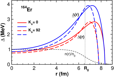
Figure 2: The pair field (gap) $\Delta_{0}(r)$, the function $\underline{\Delta}=|V_{0}|I_{pp}^{\kappa\Delta}(r)$ and the nuclear density $n(r)$ as the functions of radius $r$. The solid lines – calculations without the spin-spin interaction $V_{ss}$, the dashed lines – $V_{ss}$ is included.

The value of $r^{\prime}$ is not fixed by the theory and can be used as the fitting parameter. We have found in our previous paper [13] that the best agreement of calculated results with experimental data is achieved at the point $r^{\prime}$ where the function $I_{pp}^{\kappa\Delta}(r^{\prime},p_{F}(r^{\prime}))$ has its maximum. Nevertheless, to get rid off the fitting parameter, we use the averaged values of these functions: $\bar{\Delta}_{0}=\int d{\bf r}\,n_{0}({\bf r})\Delta_{0}(r,p_{F}(r))/A$, etc. The gap $\Delta(r,p_{F}(r))$, as well as the integrals $I^{\kappa\Delta}_{pp}(r,p_{F}(r))$, ${\cal K}_{4}$ and ${\cal K}_{0}$, were calculated with the help of the semiclassical formulae for $\kappa({\bf r},{\bf p})$ and $\Delta({\bf r},{\bf p})$ (see Appendix D), a Gaussian being used for the pairing interaction with $r_{p}=1.9$ fm and $V_{0}=25$ MeV [17]. Those values reproduce usual nuclear pairing gaps.

$\bullet$ The used spin-spin interaction is repulsive, the values of its strength constants being taken from the paper [23], where the notation $\chi=K_{s}/A,\,\bar{\chi}=q\chi$ was introduced. The constants were extracted by the authors of [23] from Skyrme forces following the standard procedure, the residual interaction being defined in terms of second derivatives of the Hamiltonian density $H(\rho)$ with respect to the one-body densities $\rho$. Different variants of Skyrme forces produce different strength constants of spin-spin interaction. The most consistent results are obtained with SG1, SG2 [24] and Sk3 [25] forces. To compare theoretical results with experiment the authors of [23] preferred to use the force SG2. Nevertheless they have noticed that ”As is well known, the energy splitting of the HF states around the Fermi level is too large. This has an effect on the spin M1 distributions that can be roughly compensated by reducing the $K_{s}$ value”. According to this remark they changed the original self-consistent SG2 parameters from $K_{s}=88$ MeV, $q=-0.95$ to $K_{s}=50$ MeV, $q=-1$. It was found that this modified set of parameters gives better agreement with experiment for some nuclei in the description of spin-flip resonance. So we will use $K_{s}=50$ MeV and $q=-1$.

$\bullet$ Our calculations without pairing [15] have shown that the results are strongly dependent on the values of the strength constants of the spin-spin interaction. The natural question arises: how sensitive are they to the strength of the spin-orbital potential? The results of the demonstrative calculations are shown in Fig. 3.

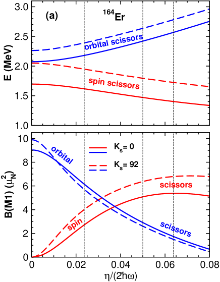
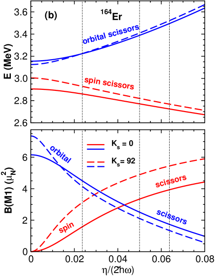
Figure 3: The energies $E$ and $B(M1)$-factors as a functions of the spin-orbital strength constant $\eta$. Left panel: solid lines – without the spin-spin interaction $V_{ss}$, dashed lines – $V_{ss}$ is included. Right panel: The same as in left panel with pair correlations included.

The $M1$ strengths were computed using effective spin giromagnetic factors $g_{s}^{eff}=0.7g_{s}^{free}$. One observes a rather strong dependence of the results on the value of $\eta$: the splitting $\Delta E$ and the $M1$ strength of the spin scissors grow with increasing $\eta$, the $B(M1)$ of the orbital scissors being decreased. At some critical point $\eta_{c}$ the $M1$ strength of the spin scissors becomes bigger than that of the orbital scissors. The inclusion of the spin-spin interaction does not change the qualitative picture, as well as the inclusion of pair correlations (see Fig. 3).

What value of $\eta$ to use? Accidentally, the choice of $\eta$ in our previous papers [14, 15] was not very realistic. The main purpose of the first paper was the introduction of spin degrees of freedom into the WFM method, and the aim of the second paper was to study the influence of spin-spin forces on both scissors – we did not worry much about the comparison with experiment. Now, both preliminary aims being achieved, one can think about the agreement with experimental data, therefore the precise choice of the model parameters becomes important. Of course, we could try to choose $\eta$ according to the standard requirement of the best agreement with experiment. However, in reality we are not absolutely free in our choice. It turns out that we are already restricted by the other constraints. As a matter of fact we work with the Nilsson potential, parameters of which are very well known. Really, the mean field of our model (9) is the deformed harmonic oscillator with the spin-orbit potential, the Nilsson $\ell^{2}$ term being neglected because it generates the fourth order moments and, anyway, they are probably not of great importance. In the original paper [26] Nilsson took the spin-orbit strength constant $\kappa_{Nils}=0.05$ for rare earth nuclei. Later the best value of $\kappa_{Nils}$ for rare earth nuclei was established [17] to be $0.0637$. For actinides there were established different values of $\kappa_{Nils}$ for neutrons ($0.0635$) and protons ($0.0577$). The numbers $\kappa_{Nils}=0.0637$, $\kappa_{Nils}=0.05$ and $\kappa_{Nils}=0.024$ (corresponding to $\eta=0.36$ used in our previous calculations [14, 15]) are marked on Figs 3, 5 by the dotted vertical lines. Of course we will use the conventional [17] parameters of the Nilsson potential and from now on we will speak only about the Nilsson [26] spin-orbital strength parameter $\kappa_{Nils}$, which is connected with $\eta$ by the relation $\eta=2\hbar\omega\kappa_{Nils}$.

5.2 Discussion and interpretation of results

The energies and excitation probabilities of orbital and spin scissors modes obtained by the solution of the isovector set of equations (4) are displayed in the Table 1.

Table 1: Scissors modes energies $E_{\rm sc}$ and transition probabilities $B(M1)_{\rm sc}$.

164Er		$E_{\rm sc}$, MeV			$B(M1)_{\rm sc},\ \mu_{N}^{2}$
		$K_{\rm s}=0$	$K_{\rm s}=50$	$K_{\rm s}=92$	$K_{\rm s}=0$	$K_{\rm s}=50$	$K_{\rm s}=92$
spin	$\bar{\Delta}_{0}=0$	1.40	1.60	1.73	5.38	6.23	6.79
scissors	$\bar{\Delta}_{0}\neq 0$	2.72	2.75	2.77	3.93	4.79	5.44
orbital	$\bar{\Delta}_{0}=0$	2.57	2.69	2.78	1.74	1.59	1.50
scissors	$\bar{\Delta}_{0}\neq 0$	3.49	3.51	3.52	1.74	1.51	1.35

There are results of calculations with three values of the spin-spin strength constant and two values of $\bar{\Delta}_{0}$. As it was expected the energies of both scissors increased approximately by 1 Mev after inclusion of pairing. The behaviour of transition probabilities turned out less predictable. The $B(M1)$ value of the spin scissors decreased approximately by 1.5 $\mu_{N}^{2}$, whereas $B(M1)$ value of the orbital scissors turned out practically insensitive to the inclusion of pair correlations.

We can compare the summed $B(M1)_{\Sigma}=B(M1)_{or}+B(M1)_{sp}$ values and the centroid of both scissors energies

$$E_{cen}=[E_{or}B(M1)_{or}+E_{sp}B(M1)_{sp}]/B(M1)_{\Sigma}$$

with the results of the paper [13] where no spin degrees of freedom had been considered and with the experimental data. The respective results are shown in the Table 2.

Table 2: Scissors modes energy centroid $E_{cen}$ and summarized transition probabilities $B(M1)_{\Sigma}$. The experimental values of $E_{cen}$, $\delta$, and $B(M1)_{\Sigma}$ are from [27] and references therein.

164Er	$E_{cen}$, MeV					$B(M1)_{\Sigma},\ \mu_{N}^{2}$
	$K_{\rm s}=0$	$K_{\rm s}=50$	$K_{\rm s}=92$	[13]	exp	$K_{\rm s}=0$	$K_{\rm s}=50$	$K_{\rm s}=92$	[13]	exp
$\bar{\Delta}_{0}=0$	1.69	1.82	1.92	2.10		7.13	7.82	8.29	9.26
					2.90					1.45
$\bar{\Delta}_{0}\neq 0$	2.96	2.93	2.92	3.37		5.67	6.30	6.79	5.62

It is seen that the inclusion of spin degrees of freedom in the WFM method does not change markedly our results (in comparison with previous ones [13]). Of course, the energy changed in the desired direction and now practically coincides with the experimental value (especially in the case with spin-spin forces.) However, the situation with the $B(M1)$ values did not change (and even become worse in the case with spin-spin forces). Our hope, that spin degrees of freedom can improve the situation with the $B(M1)$ values, did not become true: the theory so far gives four times bigger values of $B(M1)$ than the experimental ones, exactly as it was the case in the paper [13].

The result look discouraging. However, a phenomenon, which was missed in our previous papers and described in the next section will save the situation.

6 Counter-rotating angular momenta of spins up/down (hidden angular momenta)

The equilibrium (ground state) orbital angular momentum of any nucleus is composed of two equal parts: half of nucleons (protons + neutrons) having spin projection up and other half having spin projection down. It is known that the huge majority of nuclei have zero angular momentum in the ground state. We will show below that as a rule this zero is just the sum of two rather big counter directed angular momenta (hidden angular momenta, because they are not manifest in the ground state) of the above mentioned two parts of any nucleus. Being connected with the spins of nucleons this phenomenon naturally has great influence on all nuclear properties connected with the spin, in particular, the spin scissors mode.

Let us analyze the procedure of linearization of the equations of motion for collective variables (23). We consider small deviations of the system from equilibrium, so all variables are written as a sum of their equilibrium value plus a small deviation:

$$L(t)=L(eq)+{\cal L}(t),\quad\mbox{et al.}$$

Neglecting quadratic deviations one obtains the set of linearized equations for deviations depending on the equilibrium values $R^{\tau\varsigma}_{\lambda\mu}(eq)$ and $L^{\tau\varsigma}_{\lambda\mu}(eq)$, which are the input data of the problem. In the paper [15] we made the following choice:

$$R^{+}_{2\pm 1}(eq)=R^{+}_{2\pm 2}(eq)=0,\quad R^{+}_{20}(eq)\neq 0,\quad R^{+}_{00}(eq)\neq 0,$$ (28)

$$R^{\uparrow\downarrow}_{\lambda\mu}(eq)=R^{\downarrow\uparrow}_{\lambda\mu}(eq)=0,$$ (29)

$$L^{\tau\varsigma}_{\lambda\mu}(eq)=0,\quad R^{-}_{\lambda\mu}(eq)=0.$$ (30)

At first glance, this choice looks quite natural. Really, relations (28) follow from the axial symmetry of nucleus. Relations (29) are justified by the fact that these quantities should be diagonal in spin at equilibrium. The variables $L^{\tau\varsigma}_{\lambda\mu}(t)$ contain the momentum ${\bf p}$ in their definition which incited us to suppose zero equilibrium values as well (we will show below that it is not true for $L^{-}_{10}$ because of quantum effects connected with spin).

The relation $R^{-}_{\lambda\mu}(eq)=0$ follows from the shell model considerations: the nucleons with spin projection ”up” and ”down” are sitting in pairs on the same levels, therefore all average properties of the ”spin up” part of nucleus must be identical to that of the ”spin down” part. However, the careful analysis shows that being undoubtedly true for variables $R^{\uparrow\uparrow}_{\lambda\mu},\,R^{\downarrow\downarrow}_{\lambda\mu}$ this statement turns out erroneous for variables $L^{\uparrow\uparrow}_{10},\,L^{\downarrow\downarrow}_{10}$. Let us demonstrate it. By definition

$$L^{ss^{\prime}}_{\lambda\mu}(t)=\int\!d^{3}r\,\int\!\frac{d^{3}p}{(2\pi\hbar)^{3}}\{r\otimes p\}_{\lambda\mu}f^{ss^{\prime}}({\bf r},{\bf p},t)=\int\!d^{3}r\{r\otimes J^{ss^{\prime}}\}_{\lambda\mu},$$ (31)

where

$$J^{ss^{\prime}}_{i}({\bf r},t)=\int\!\frac{d^{3}p}{(2\pi\hbar)^{3}}p_{i}f^{ss^{\prime}}({\bf r},{\bf p},t)=\int\!\frac{d^{3}p}{(2\pi\hbar)^{3}}p_{i}\int\!d^{3}q\exp(-\frac{i}{\hbar}{\bf p}\cdot{\bf q})\rho({\bf r}+\frac{{\bf q}}{2},s;{\bf r}-\frac{{\bf q}}{2},s^{\prime};t)$$ (32)

is the i-th component of the nuclear current. In the last relation the definition [17] of Wigner function is used. Performing the integration over ${\bf p}$ one finds:

$$J^{ss^{\prime}}_{i}({\bf r},t)=i\hbar\int\!d^{3}q[\frac{\partial}{\partial q_{i}}\delta({\bf q})]\rho({\bf r}+\frac{{\bf q}}{2},s;{\bf r}-\frac{{\bf q}}{2},s^{\prime};t)$$

$$=-i\hbar\int\!d^{3}q\delta({\bf q})\frac{\partial}{\partial q_{i}}\rho({\bf r}+\frac{{\bf q}}{2},s;{\bf r}-\frac{{\bf q}}{2},s^{\prime};t)$$

$$=-\frac{i\hbar}{2}[(\nabla_{1i}-\nabla_{2i})\rho({\bf r}_{1},s;{\bf r}_{2},s^{\prime};t)]_{{\bf r}_{1}={\bf r}_{2}={\bf r}},$$ (33)

where ${\bf r}_{1}={\bf r}+\frac{{\bf q}}{2},\,{\bf r}_{2}={\bf r}-\frac{{\bf q}}{2}$. The density matrix of the ground state nucleus is defined [17] as

$$\rho({\bf r}_{1},s;{\bf r}_{2},s^{\prime};t)=\sum_{\nu}v^{2}_{\nu}\phi_{\nu}({\bf r}_{1}s)\phi^{*}_{\nu}({\bf r}_{2}s^{\prime}),$$ (34)

where $v^{2}_{\nu}$ are occupation numbers and $\phi_{\nu}$ are single particle wave functions. For the sake of simplicity we will consider the case of spherical symmetry. Then $\nu=nljm$ and

$$\phi_{nljm}({\bf r},s)={\cal R}_{nlj}(r)\sum_{\Lambda,\sigma}C^{jm}_{l\Lambda,\frac{1}{2}\sigma}Y_{l\Lambda}(\theta,\phi)\chi_{\frac{1}{2}\sigma}(s),$$ (35)

$$J^{ss^{\prime}}_{i}({\bf r})=-\frac{i\hbar}{2}\sum_{\nu}v^{2}_{\nu}[\nabla_{i}\phi_{\nu}({\bf r},s)\cdot\phi^{*}_{\nu}({\bf r},s^{\prime})-\phi_{\nu}({\bf r},s)\cdot\nabla_{i}\phi^{*}_{\nu}({\bf r},s^{\prime})]$$ (36)

$$=-\frac{i\hbar}{2}\sum_{nljm}v^{2}_{nljm}{\cal R}^{2}_{nlj}\sum_{\Lambda,\sigma,\Lambda^{\prime},\sigma^{\prime}}C^{jm}_{l\Lambda,\frac{1}{2}\sigma}C^{jm}_{l\Lambda^{\prime},\frac{1}{2}\sigma^{\prime}}[Y^{*}_{l\Lambda^{\prime}}\nabla_{i}Y_{l\Lambda}-Y_{l\Lambda}\nabla_{i}Y^{*}_{l\Lambda^{\prime}}]\chi_{\frac{1}{2}\sigma}(s)\chi_{\frac{1}{2}\sigma^{\prime}}(s^{\prime}).$$ (37)

Inserting this expression into (31) one finds:

$$L^{ss^{\prime}}_{10}(eq)=-\frac{i\hbar}{2}\sum_{nljm}v^{2}_{nljm}\sum_{\Lambda\sigma,\Lambda^{\prime}\sigma^{\prime}}C^{jm}_{l\Lambda,\frac{1}{2}\sigma}C^{jm}_{l\Lambda^{\prime},\frac{1}{2}\sigma^{\prime}}\chi_{\frac{1}{2}\sigma}(s)\chi_{\frac{1}{2}\sigma^{\prime}}(s^{\prime})$$

$$\int\!d^{3}r\,{\cal R}^{2}_{nlj}[Y^{*}_{l\Lambda^{\prime}}\{r\otimes\nabla\}_{10}Y_{l\Lambda}-Y_{l\Lambda}\{r\otimes\nabla\}_{10}Y^{*}_{l\Lambda^{\prime}}]$$

$$=\frac{i}{2\sqrt{2}}\sum_{nljm}v^{2}_{nljm}\sum_{\Lambda\sigma,\Lambda^{\prime}\sigma^{\prime}}C^{jm}_{l\Lambda,\frac{1}{2}\sigma}C^{jm}_{l\Lambda^{\prime},\frac{1}{2}\sigma^{\prime}}\chi_{\frac{1}{2}\sigma}(s)\chi_{\frac{1}{2}\sigma^{\prime}}(s^{\prime})\int\!d^{3}r\,{\cal R}^{2}_{nlj}[Y^{*}_{l\Lambda^{\prime}}\hat{l}_{0}Y_{l\Lambda}-Y_{l\Lambda}\hat{l}_{0}Y^{*}_{l\Lambda^{\prime}}]$$

$$=\frac{i}{2\sqrt{2}}\sum_{nljm}v^{2}_{nljm}\sum_{\Lambda\sigma,\Lambda^{\prime}\sigma^{\prime}}C^{jm}_{l\Lambda,\frac{1}{2}\sigma}C^{jm}_{l\Lambda^{\prime},\frac{1}{2}\sigma^{\prime}}\chi_{\frac{1}{2}\sigma}(s)\chi_{\frac{1}{2}\sigma^{\prime}}(s^{\prime})(\Lambda+\Lambda^{\prime})\delta_{\Lambda,\Lambda^{\prime}}$$

$$=\frac{i}{\sqrt{2}}\sum_{nljm}v^{2}_{nljm}\sum_{\Lambda\sigma}\Lambda\,\left(C^{jm}_{l\Lambda,\frac{1}{2}\sigma}\right)^{2}\chi_{\frac{1}{2}\sigma}(s)\chi_{\frac{1}{2}\sigma}(s^{\prime}).$$ (38)

Here the definition $\hat{l}_{\mu}=-\hbar\sqrt{2}\{r\otimes\nabla\}_{1\mu}$, formula $\hat{l}_{0}Y_{l\Lambda}=\Lambda Y_{l\Lambda}$ and normalization of functions ${\cal R}_{nlj}$ were used. Remembering the definition of the spin function $\chi_{\frac{1}{2}\sigma}(s)=\delta_{\sigma,s}$ we get finally:

$$L^{ss^{\prime}}_{10}(eq)=\frac{i}{\sqrt{2}}\sum_{nljm}v^{2}_{nljm}\sum_{\Lambda}\Lambda\,\left(C^{jm}_{l\Lambda,\frac{1}{2}s}\right)^{2}\delta_{s,s^{\prime}}=\delta_{s,s^{\prime}}\frac{i}{\sqrt{2}}\sum_{nljm}v^{2}_{nljm}\left(C^{jm}_{lm-s,\frac{1}{2}s}\right)^{2}(m-s).$$ (39)

Now, with the help of analytic expressions for Clebsh-Gordan coefficients one obtains the final expressions

$$L^{\uparrow\uparrow}_{10}(eq)=\frac{i}{\sqrt{2}}\sum_{nl}\left[\sum_{m=-\left(l+\frac{1}{2}\right)}^{l+\frac{1}{2}}v^{2}_{nlj^{+}m}\frac{l+\frac{1}{2}+m}{2l+1}+\sum_{m=-\left(l-\frac{1}{2}\right)}^{l-\frac{1}{2}}v^{2}_{nlj^{-}m}\frac{l+\frac{1}{2}-m}{2l+1}\right]\left(m-\frac{1}{2}\right),$$ (40)

$$L^{\downarrow\downarrow}_{10}(eq)=\frac{i}{\sqrt{2}}\sum_{nl}\left[\sum_{m=-\left(l+\frac{1}{2}\right)}^{l+\frac{1}{2}}v^{2}_{nlj^{+}m}\frac{l+\frac{1}{2}-m}{2l+1}+\sum_{m=-\left(l-\frac{1}{2}\right)}^{l-\frac{1}{2}}v^{2}_{nlj^{-}m}\frac{l+\frac{1}{2}+m}{2l+1}\right]\left(m+\frac{1}{2}\right),$$ (41)

where the notation $j^{\pm}=l\pm\frac{1}{2}$ is introduced. Replacing in (40) $m$ by $-m$ we find that

$$L^{\uparrow\uparrow}_{10}(eq)=-L^{\downarrow\downarrow}_{10}(eq).$$ (42)

By definition (23) $L^{\pm}_{10}(eq)=L^{\uparrow\uparrow}_{10}(eq)\pm L^{\downarrow\downarrow}_{10}(eq)$. Combining linearly (40) and (41) one finds:

$$L^{+}_{10}(eq)=\frac{i}{\sqrt{2}}\sum_{nl}\left[\sum_{m=-\left(l+\frac{1}{2}\right)}^{l+\frac{1}{2}}v^{2}_{nlj^{+}m}\frac{2l}{2l+1}m+\sum_{m=-\left(l-\frac{1}{2}\right)}^{l-\frac{1}{2}}v^{2}_{nlj^{-}m}\frac{2l+2}{2l+1}m\right],$$ (43)

$$L^{-}_{10}(eq)=\frac{i}{\sqrt{2}}\sum_{nl}\left[\sum_{m=-\left(l+\frac{1}{2}\right)}^{l+\frac{1}{2}}v^{2}_{nlj^{+}m}\frac{2m^{2}-l-\frac{1}{2}}{2l+1}-\sum_{m=-\left(l-\frac{1}{2}\right)}^{l-\frac{1}{2}}v^{2}_{nlj^{-}m}\frac{2m^{2}+l+\frac{1}{2}}{2l+1}\right].$$ (44)

These formulas are valid for spherical nuclei. However, with the scissors and spin-scissors modes, we are considering deformed nuclei. For the sake of the discussion, let us consider the case of infinitesimally small deformation, when one can continue to use formulae (43, 44). Now only levels with quantum numbers $\pm m$ are degenerate. According to, for example, the Nilsson scheme [26] nucleons will occupy pairwise precisely those levels which leads to the zero value of $L^{+}_{10}(eq)$.

What about $L^{-}_{10}(eq)$? It only enters (27) in the equation for $\dot{{\cal P}}^{-}_{21}$. Let us analyze the structure of formula (44) considering for the sake of simplicity the case without pairing. Two sums over $m$ (let us note them $\Sigma_{1}$ and $\Sigma_{2}$) represent two spin-orbital partners: in the first sum the summation goes over levels of the lower partner ($j=l+\frac{1}{2}$) and in the second sum – over levels of the higher partner ($j=l-\frac{1}{2}$). The values of both sums depend naturally on the values of occupation numbers $n_{nljm}=0,1$. There are three possibilities. The first one is trivial: if all levels of both spin-orbital partners are disposed above the Fermi surface, then the respective occupation numbers $n_{nljm}=0$ and both sums are equal to zero identically. The second possibility: all levels of both spin-orbital partners are disposed below the Fermi surface. Then all respective occupation numbers $n_{nlj^{+}m}=n_{nlj^{-}m}=1$. The elementary analytical calculation (for arbitrary $l$) shows that in this case the two sums in (44) exactly compensate each other, i.e. $\Sigma_{1}+\Sigma_{2}=0$. The most interesting is the third possibility, when one part of levels of two spin-orbital partners is disposed below the Fermi surface and another part is disposed above it. In this case the compensation does not happen and one gets $\Sigma_{1}+\Sigma_{2}\neq 0$ what leads to $L^{-}_{10}(eq)\neq 0$. In the case of pairing, things are not so sharply separated and $L_{10}^{-}(eq)$ has always a finite value. However, the modifications with respect to mean field are very small.

Let us illustrate the above analysis by the example of ¹⁶⁴Er (protons). Its deformation is $\delta=0.25$ $(\epsilon=0.26)$ and Z=68. Looking on the Nilsson scheme (for example, Fig.1.5 of [16] or Fig. 2.21c of [17]) one easily finds, that only three pairs of spin-orbital partners give a nonzero contribution to $L^{-}_{10}(eq)$. They are: $N=4,d_{5/2}-d_{3/2}$ (two levels of $d_{5/2}$ are below the Fermi surface, all the rest – above); $N=4,g_{9/2}-g_{7/2}$ (one level of $g_{7/2}$ is above the Fermi surface, all the rest – below); $N=5,h_{11/2}-h_{9/2}$ (four levels of $h_{11/2}$ are below the Fermi surface, all the rest – above). It is possible to make the crude evaluation of $L^{-}_{10}(eq)$ using the quantum numbers indicated on Fig.1.5 of [16] or Fig. 2.21c of [17]). The result turns out rather close to the exact one, computed with the help of formulas (31,36) and Nilsson wave functions. The influence of pair correlations is very small.

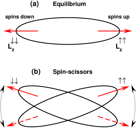
Figure 4: (a) Protons with spins $\uparrow$ (up) and $\downarrow$ (down) having nonzero orbital angular momenta at equilibrium. (b) Protons from Fig.(a) vibrating against one-another.

Indeed, from the definitions (31) and (38) one can see that $L^{ss}_{10}(eq)$ is just the average value of the z-component of the orbital angular momentum of nucleons with the spin projection $s$ ($\frac{1}{2}$ or $-\frac{1}{2}$). So, the ground state nucleus consists of two equal parts having nonzero angular momenta with opposite directions, which compensate each other resulting in the zero total angular momentum. This is graphically depicted in Fig. 4(a).

On the other hand, when the opposite angular momenta become tilted, one excites the system and the opposite angular momenta are vibrating with a tilting angle, see Fig. 4(b). Actually the two opposite angular momenta are oscillating, one in the opposite sense of the other. It is rather obvious from Fig. 1 that these tilted vibrations happen separately in each of the neutron and proton lobes. These spin-up against spin-down motions certainly influence the excitation of the spin scissors mode. So, classically speaking the proton and neutron parts of the ground state nucleus consist each of two identical gyroscopes rotating in opposite directions. One knows that it is very difficult to deviate gyroscope from an equilibrium. So one can expect, that the probability to force two gyroscopes to oscillate as scissors (spin scissors) should be small. This picture is confirmed in the next section.

7 Results of calculations continued

We made the calculations taking into account the non zero value of $L_{10}^{-}(eq)$ (which was computed according to formulas (31,36) and Nilsson wave functions). The results are shown on Fig. 5.

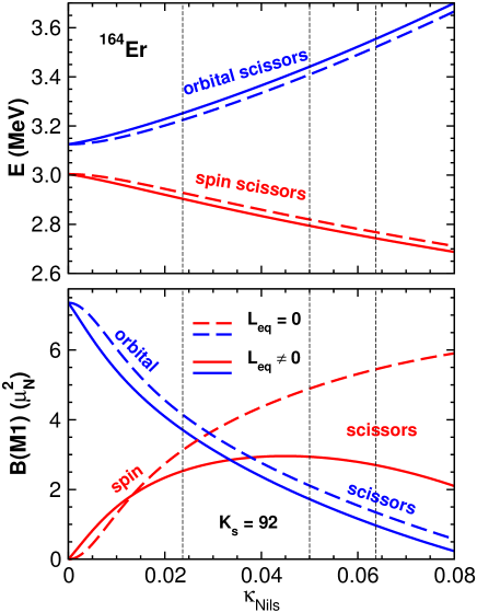
Figure 5: The energies $E$ and $B(M1)$-factors as a functions of the spin-orbital strength constant $\kappa_{Nils}$. The dashed lines – calculations without $L_{10}^{-}(eq)$, the solid lines – $L_{10}^{-}(eq)$ are taken into account. $V_{ss}$ and pairing are included.

They demonstrate (in comparison with Fig. 3) the strong influence of the spin-up vs spin-down angular momenta on the spin scissors mode, whose B(M1) value is strongly decreasing with increasing $\kappa_{Nils}$. The B(M1) value of the orbital scissors also is reduced, but not so much, the value of the reduction being practically independent on $\kappa_{Nils}$. The influence of $L_{10}^{-}(eq)$ on the energies of both scissors is negligible, leading to the small increase of their splitting. Now the energy centroid of both scissors and their summed B(M1) value at $\kappa_{Nils}=0.0637$ are $E_{cen}=2.97$ MeV and $B(M1)_{\Sigma}=3.7\mu_{N}^{2}$. The general agreement with experiment becomes considerably better (compare with Table 2), though the theoretical value of $B(M1)_{\Sigma}$ still exceeds the experimental one approximately 2.5 times. However, as we will see, the case of ¹⁶⁴Er may imply a quite particular situation (or even a problem with the experimental value).

The results of systematic calculations for rare-earth nuclei are presented in Tables 3 and 4 and desplayed in Fig. 6. Table 3 contains the results for well deformed nuclei with $\delta\geq 0.18.$ It is easy to see that the overall (general) agreement of theoretical results with experimental data is substantially improved (in comparison with our previous calculations [13]).

Table 3: Scissors modes energy centroid $E_{\rm cen}$ and summarized transition probabilities $B(M1)_{\Sigma}$. Parameters: $\kappa_{Nils}=0.0637$, $V_{0}=25$ ($V_{0}=27$ for ^182,184,186W). The experimental values of $E_{\rm cen}$, $\delta$, and $B(M1)_{\Sigma}$ are from [27] and references therein.

		$E_{\rm cen}$, MeV				$B(M1)_{\Sigma},\ \mu_{N}^{2}$
Nuclei	$\delta$	exp	present	[13]	$\Delta=0$	exp	present	[13]	$\Delta=0$
150Nd	0.22	3.04	2.88	3.44	1.92	1.61	1.64	4.17	7.26
152Sm	0.24	2.99	2.99	3.46	2.02	2.26	2.50	4.68	7.81
154Sm	0.26	3.20	3.10	3.57	2.17	2.18	3.34	5.42	8.65
156Gd	0.26	3.06	3.09	3.60	2.16	2.73	3.44	5.42	8.76
158Gd	0.26	3.14	3.09	3.60	2.19	3.39	3.52	5.72	9.12
160Gd	0.27	3.18	3.14	3.61	2.21	2.97	4.02	5.90	9.38
160Dy	0.26	2.87	3.08	3.59	2.13	2.42	3.60	5.53	9.03
162Dy	0.26	2.96	3.07	3.61	2.14	2.49	3.69	5.66	9.25
164Dy	0.26	3.14	3.07	3.60	2.17	3.18	3.78	5.95	9.59
164Er	0.25	2.90	3.01	3.57	2.10	1.45	3.39	5.62	9.26
166Er	0.26	2.96	3.06	3.53	2.13	2.67	3.86	5.96	9.59
168Er	0.26	3.21	3.06	3.53	2.10	2.82	3.95	5.95	9.67
170Er	0.26	3.22	3.05	3.57	2.09	2.63	4.03	5.91	9.79
172Yb	0.25	3.03	2.99	3.55	2.05	1.94	3.72	5.84	9.79
174Yb	0.25	3.15	2.98	3.47	2.02	2.70	3.80	5.89	9.82
176Yb	0.24	2.96	2.92	3.45	1.94	2.66	3.46	5.54	9.58
178Hf	0.22	3.11	2.81	3.43	1.79	2.04	2.67	4.86	9.00
180Hf	0.22	2.95	2.81	3.36	1.76	1.61	2.69	4.85	8.97
182W	0.20	3.10	3.28	3.30	1.63	1.65	2.05	4.31	8.43
184W	0.19	3.31	3.24	3.28	1.55	1.12	1.72	3.97	8.14
186W	0.18	3.20	3.19	3.26	1.49	0.82	1.40	3.76	7.95

Table 4: Scissors modes energy centroid $E_{\rm cen}$ and summarized transition probabilities $B(M1)_{\Sigma}$. Parameters: $\kappa=0.05$ ($\kappa=0.0637$ for ^182,184,186W), $V_{0}=27$.

		$E_{\rm cen}$, MeV				$B(M1)_{\Sigma},\ \mu_{N}^{2}$
Nuclei	$\delta$	exp	present	[13]	$\Delta=0$	exp	present	[13]	$\Delta=0$
134Ba	0.14	2.99	3.04	3.09	1.28	0.56	0.68	1.67	3.90
148Nd	0.17	3.37	3.22	3.18	1.48	0.78	1.28	2.58	5.39
150Sm	0.16	3.13	3.17	3.13	1.42	0.92	1.12	2.45	5.26
182W	0.20	3.10	3.28	3.30	1.63	1.65	2.05	4.31	8.43
184W	0.19	3.31	3.24	3.28	1.55	1.12	1.72	3.97	8.14
186W	0.18	3.20	3.19	3.26	1.49	0.82	1.40	3.76	7.95
190Os	0.15	2.90	3.14	3.12	1.21	0.98	1.38	2.67	6.64
192Os	0.14	3.01	3.11	3.12	1.15	1.04	1.00	2.42	6.37

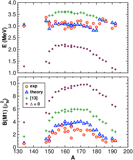
Figure 6: The energies $E_{sc}$ and $B(M1)_{sc}$-factors as a function of the mass number A for nuclei listed in the Table 3.

The results of calculations for two groups (”light” and ”heavy”) of weakly deformed nuclei with deformations $0.14\leq\delta\leq 0.17$ are shown in the Table 4. They require some discussion, because of the self-consistency problem. These two groups of nuclei are transitional between well deformed and spherical nuclei. Systematic calculations of equilibrium deformations [16] predict $\delta_{eq}^{th}=0.0$ for ¹³⁴Ba, $\pm 0.1$ for ¹⁴⁸Nd, 0.15 or -0.12 for ¹⁵⁰Sm, 0.1 or -0.14 for ¹⁹⁰Os and -0.1 for ¹⁹²Os, whereas their experimental values are $\delta_{eq}=0.14,\,0.17,\,0.16,\,0.15$ and 0.14 respectively. As one sees, the discrepancy between theoretical and experimental $\delta_{eq}$ is large. Uncertain signs of theoretical equilibrium deformations are connected with very small ($\sim$0.1-0.2 MeV) difference between the values of deformation energies ${\cal E}_{def}$ at positive and negative $\delta_{eq}$. Even more so, the values of deformation energies of these nuclei are very small: ${\cal E}_{def}=0.20,~{}0.50,~{}0.80$ and 0.70 MeV for ¹⁴⁸Nd, ¹⁵⁰Sm, ¹⁹⁰Os and ¹⁹²Os respectively. This means that these nuclei are very ”soft” with respect of $\beta$- or $\gamma$-vibrations and probably they have more complicated equilibrium shapes, for example, hexadecapole or octupole deformations in addition to the quadrupole one. This means that for the correct description of their dynamical and equilibrium properties it is necessary to include higher order Wigner function moments (at least fourth order) in addition to the second order ones. In this case it would be natural also to use more complicate mean field potentials (for example, the Woods-Saxon one or the potential extracted from some of the numerous variants of Skyrme forces) instead of the too simple Nilsson potential. Naturally, this will be the subject of further investigations. However, to be sure that the situation with these nuclei is not absolutely hopeless, one can try to imitate the properties of the more perfect potential by fitting parameters of the Nilsson potential. As a matter of fact this potential has the single but essential parameter – the spin-orbital strength $\kappa_{Nils}$. It turns out that changing its value from 0.0637 to 0.05 (the value used by Nilsson in his original paper [26]) is enough to obtain the reasonable description of B(M1) factors (see Table 4). To obtain the reasonable description of the scissors energies we use the ”freedom” of choosing the value of the pairing interaction constant $V_{0}$ in (21). It turns out that changing its value from 25 MeV to 27 MeV is enough to obtain the satisfactory agreement between the theoretical and experimental values of $E_{sc}$ (Table 4).

The isotopes ^182-186W turn out intermediate between weakly deformed and well deformed nuclei: reasonable results are obtained with $\kappa_{Nils}=0.0637$ (as for well deformed) and $V_{0}=27$ MeV (as for weakly deformed). That is why they appear in both Tables.

Returning to the group of well deformed nuclei with $\delta\geq 0.18$ (Table 3) it is necessary to emphasize that all presented results for these nuclei were obtained without any fitting. In spite of it the agreement between the theory and experiment can be called excellent for all nuclei of this group except two: ¹⁶⁴Er and ¹⁷²Yb, where the theory overestimates B(M1) values approximately two times. However, these two nuclei fall out of the systematics and one can suspect, that there the experimental B(M1) values are underestimated. Therefore one can hope, that new experiments will correct the situation with these nuclei, as it happened, for example, with ²³²Th [28].

8 Conclusion

The method of Wigner function moments is generalized to take into account spin degrees of freedom and pair correlations simultaneously. The inclusion of the spin into the theory allows one to discover several new phenomena. One of them, the nuclear spin scissors, was described and studied in [14, 15], where some indications on the experimental confirmation of its existence in actinides nuclei are discussed. Another phenomenon, the opposite rotation of spin up/down nucleons, or in other words, the phenomenon of hidden angular momenta, is described in this paper. Being determined by the spin degrees of freedom this phenomenon has great influence on the excitation probability of the spin scissors mode. On the other hand the spin scissors B(M1) values and the energies of both, spin and orbital, scissors are very sensitive to the action of pair correlations. As a result, these two factors, the spin up/down counter-rotation and pairing, working together, improve substantially the agreement between the theory and experiment in the description of the energy centroid of two nuclear scissors and their summed excitation probability. More precisely, for the first time an excellent agreement is achieved for well deformed nuclei of the rare earth region with standard values of all possible parameters.

An excellent agreement is also achieved for weakly deformed (transitional) nuclei of the same region by a very modest re-fit of the spin-orbit strength. We suppose that fourth order moments and more realistic interactions are required for the adequate description of transitional nuclei. However this shall be the subject of future work.

Acknowledgements
Valuable discussions with V. N. Kondratyev are gratefully acknowledged.

Appendix A

Abnormal density

According to formula (D.47) of [17] the abnormal density in coordinate representation $\kappa({\bf r},s;{\bf r}^{\prime},s^{\prime})$ is connected with the abnormal density in the representation of the harmonic oscillator quantum numbers $\kappa_{\nu,\nu^{\prime}}=\langle\Phi|a_{\nu}a_{\nu^{\prime}}|\Phi\rangle$ by the relation

$$\kappa({\bf r},s;{\bf r}^{\prime},s^{\prime})=\langle\Phi|a({\bf r},s)a({\bf r}^{\prime},s^{\prime})|\Phi\rangle=\sum_{\nu,\nu^{\prime}}\psi_{\nu}({\bf r},s)\psi_{\nu^{\prime}}({\bf r}^{\prime},s^{\prime})\langle\Phi|a_{\nu}a_{\nu^{\prime}}|\Phi\rangle,$$ (A.1)

where

$$\nu\equiv k,\varsigma,\quad k\equiv n,l,j,|m|,\quad\varsigma={\rm sign}(m)=\pm,\quad k,+\equiv\nu,\quad k,-\equiv\bar{\nu},$$

$$\psi_{\bar{\nu}}({\bf r},s)=T\psi_{\nu}({\bf r},s).$$

$T$ - time reversal operator defined by formula (XV.85) of [29]

$$T=-i\sigma_{y}K_{0},$$

where $\sigma_{y}$ is the Pauli matrix and $K_{0}$ is the complex-conjugation operator.

According to formula (7.12) of [17]

$$a_{k,\varsigma}=u_{k}\alpha_{k,\varsigma}-\varsigma v_{k}\alpha^{\dagger}_{k,-\varsigma},$$

$$\alpha_{\nu}|\Phi\rangle=0,$$

$$\langle\Phi|a_{\nu}a_{\nu^{\prime}}|\Phi\rangle\equiv\kappa_{\nu\nu^{\prime}}=-\varsigma^{\prime}u_{k}v_{k^{\prime}}\langle\Phi|\alpha_{k,\varsigma}\alpha^{\dagger}_{k^{\prime},-\varsigma^{\prime}}|\Phi\rangle=-\varsigma^{\prime}u_{k}v_{k^{\prime}}\delta_{k,k^{\prime}}\delta_{-\varsigma,\varsigma^{\prime}}.$$ (A.2)

This result means that in accordance with the theorem of Bloch and Messiah we have found the basis $|\nu\rangle$ in which the abnormal density $\kappa_{\nu,\nu^{\prime}}$ has the canonical form. Therefore the spin structure of $\kappa_{\nu,\nu^{\prime}}$ is

$$\kappa_{\nu,\nu^{\prime}}={\qquad 0\;\qquad u_{k}v_{k}\choose-u_{k}v_{k}\;\qquad 0\qquad},$$ (A.3)

or $\kappa_{\bar{\nu},\nu}=-\kappa_{\nu,\bar{\nu}}$ and $\kappa_{\nu,\nu}=\kappa_{\bar{\nu},\bar{\nu}}=0.$

With the help of (A.2) formula (A.1) can be transformed into

$$\kappa({\bf r},s;{\bf r}^{\prime},s^{\prime}) = \sum_{k,\varsigma}\varsigma u_{k}v_{k}\psi_{k,\varsigma}({\bf r},s)\psi_{k,-\varsigma}({\bf r}^{\prime},s^{\prime})$$ (A.4)

$$= \sum_{\nu>0}u_{\nu}v_{\nu}[\psi_{\nu}({\bf r},s)\psi_{\bar{\nu}}({\bf r}^{\prime},s^{\prime})-\psi_{\bar{\nu}}({\bf r},s)\psi_{\nu}({\bf r}^{\prime},s^{\prime})].$$

that reproduces formula (D.48) of [17].

What is the spin structure of $\kappa({\bf r},s;{\bf r}^{\prime},s^{\prime})$?

Let us consider the spherical case:

$$\psi_{\nu}({\bf r},s)={\cal R}_{nlj}(r)\sum_{\Lambda,\sigma}C^{jm}_{l\Lambda,\frac{1}{2}\sigma}Y_{l\Lambda}(\theta,\phi)\chi_{\frac{1}{2}\sigma}(s)\equiv{\cal R}_{nlj}(r)\phi_{ljm}(\Omega,s),$$

where $\phi_{ljm}(\Omega,s)=\sum_{\Lambda,\sigma}C^{jm}_{l\Lambda,\frac{1}{2}\sigma}Y_{l\Lambda}(\theta,\phi)\chi_{\frac{1}{2}\sigma}(s)$, spin function $\chi_{\frac{1}{2}\sigma}(s)=\delta_{\sigma,s}$ and angular variables are denoted by $\Omega$.

Time reversal:

$$TY_{l\Lambda}=Y^{*}_{l\Lambda}=(-1)^{\Lambda}Y_{l-\Lambda},$$

$$T\chi_{\frac{1}{2}\frac{1}{2}}=\chi_{\frac{1}{2}-\frac{1}{2}},\quad T\chi_{\frac{1}{2}-\frac{1}{2}}=-\chi_{\frac{1}{2}\frac{1}{2}}\quad\to\quad T\chi_{\frac{1}{2}\sigma}=(-1)^{\sigma-\frac{1}{2}}\chi_{\frac{1}{2}-\sigma},$$

$$T\sum_{\Lambda,\sigma}C^{jm}_{l\Lambda,\frac{1}{2}\sigma}Y_{l\Lambda}\chi_{\frac{1}{2}\sigma}=\sum_{\Lambda,\sigma}C^{jm}_{l\Lambda,\frac{1}{2}\sigma}Y_{l-\Lambda}\chi_{\frac{1}{2}-\sigma}(-1)^{\Lambda+\sigma-\frac{1}{2}}=\sum_{\Lambda,\sigma}C^{jm}_{l-\Lambda,\frac{1}{2}-\sigma}Y_{l\Lambda}\chi_{\frac{1}{2}\sigma}(-1)^{-\Lambda-\sigma-\frac{1}{2}}$$

$$=\sum_{\Lambda,\sigma}C^{j-m}_{l\Lambda,\frac{1}{2}\sigma}Y_{l\Lambda}\chi_{\frac{1}{2}\sigma}(-1)^{l+\frac{1}{2}-j-\Lambda-\sigma-\frac{1}{2}}=\sum_{\Lambda,\sigma}C^{j-m}_{l\Lambda,\frac{1}{2}\sigma}Y_{l\Lambda}\chi_{\frac{1}{2}\sigma}(-1)^{l-j+m}.$$

As a result

$$\psi_{\bar{\nu}}({\bf r},s)=(-1)^{l-j+m}{\cal R}_{nlj}(r)\sum_{\Lambda,\sigma}C^{j-m}_{l\Lambda,\frac{1}{2}\sigma}Y_{l\Lambda}(\theta,\phi)\chi_{\frac{1}{2}\sigma}(s)=(-1)^{l-j+m}{\cal R}_{nlj}(r)\phi_{lj-m}(\Omega,s),$$ (A.5)

that coincides with formula (2.45) of [17]. Formula (A.4) can be rewritten now as

$$\kappa({\bf r}_{1},s_{1};{\bf r}_{2},s_{2})=\sum_{nljm>0}(uv)_{nljm}{\cal R}_{nlj}(r_{1}){\cal R}_{nlj}(r_{2})(-1)^{l-j+m}$$

$$\left[\phi_{ljm}(\Omega_{1},s_{1})\phi_{lj-m}(\Omega_{2},s_{2})-\phi_{ljm}(\Omega_{2},s_{2})\phi_{lj-m}(\Omega_{1},s_{1})\right]$$

$$=\sum_{nljm>0}(uv)_{nljm}{\cal R}_{nlj}(r_{1}){\cal R}_{nlj}(r_{2})(-1)^{l-j+m}\sum_{\Lambda,\Lambda^{\prime}}$$

$$\left[C^{jm}_{l\Lambda,\frac{1}{2}s_{1}}C^{j-m}_{l\Lambda^{\prime},\frac{1}{2}s_{2}}Y_{l\Lambda}(\Omega_{1})Y_{l\Lambda^{\prime}}(\Omega_{2})-C^{jm}_{l\Lambda,\frac{1}{2}s_{2}}C^{j-m}_{l\Lambda^{\prime},\frac{1}{2}s_{1}}Y_{l\Lambda}(\Omega_{2})Y_{l\Lambda^{\prime}}(\Omega_{1})\right]$$

$$=\sum_{nljm>0}(uv)_{nljm}{\cal R}_{nlj}(r_{1}){\cal R}_{nlj}(r_{2})(-1)^{l-j+m}\sum_{\Lambda,\Lambda^{\prime}}Y_{l\Lambda}(\Omega_{1})Y_{l\Lambda^{\prime}}(\Omega_{2})$$

$$\left[C^{jm}_{l\Lambda,\frac{1}{2}s_{1}}C^{j-m}_{l\Lambda^{\prime},\frac{1}{2}s_{2}}-C^{jm}_{l\Lambda^{\prime},\frac{1}{2}s_{2}}C^{j-m}_{l\Lambda,\frac{1}{2}s_{1}}\right].$$ (A.6)

It is obvious that $\kappa({\bf r},\uparrow;{\bf r}^{\prime},\downarrow)\neq-\kappa({\bf r},\downarrow;{\bf r}^{\prime},\uparrow)$, i.e. in the coordinate representation the spin structure of $\kappa$ has nothing common with (A.3).

The anomalous density defined by (A.6) has not definite angular momentum $J$ and spin $S$. It can be represented as the sum of several terms with definite $J,S$. We have:

$$\phi_{ljm}(1)\phi_{lj-m}(2)=\sum_{0\leq J\leq 2j}C^{J0}_{jm,j-m}\{\phi_{j}(1)\otimes\phi_{j}(2)\}_{J0}$$

$$=C^{00}_{jm,j-m}\{\phi_{j}(1)\otimes\phi_{j}(2)\}_{00}+\sum_{1\leq J\leq 2j}C^{J0}_{jm,j-m}\{\phi_{j}(1)\otimes\phi_{j}(2)\}_{J0}.$$ (A.7)

We are interested in the monopole pairing only, so we omit all terms except the first one:

$$\left[\phi_{ljm}(1)\phi_{lj-m}(2)\right]_{J=0}=C^{00}_{jm,j-m}\{\phi_{j}(1)\otimes\phi_{j}(2)\}_{00}$$

$$=(-1)^{j-m}\frac{1}{\sqrt{2j+1}}\sum_{\nu,\sigma}C^{00}_{j\nu,j\sigma}\phi_{j\nu}(1)\phi_{j\sigma}(2)$$

$$=\frac{1}{2j+1}\sum_{\nu}(-1)^{\nu-m}\phi_{j\nu}(1)\phi_{j-\nu}(2).$$ (A.8)

Remembering the definition of $\phi$ function we find

$$(-1)^{m}\left[\phi_{ljm}(\Omega_{1},s_{1})\phi_{lj-m}(\Omega_{2},s_{2})\right]_{J=0}=\frac{1}{2j+1}\sum_{\nu}(-1)^{\nu}$$

$$\sum_{\Lambda,\sigma}\sum_{\Lambda^{\prime},\sigma^{\prime}}C^{j\nu}_{l\Lambda,\frac{1}{2}\sigma}C^{j-\nu}_{l\Lambda^{\prime},\frac{1}{2}\sigma^{\prime}}Y_{l\Lambda}(\Omega_{1})Y_{l\Lambda^{\prime}}(\Omega_{2})\chi_{\frac{1}{2}\sigma}(s_{1})\chi_{\frac{1}{2}\sigma^{\prime}}(s_{2}).$$ (A.9)

The direct product of spin functions in this formula can be written as

$$\chi_{\frac{1}{2}\sigma}(s_{1})\chi_{\frac{1}{2}\sigma^{\prime}}(s_{2})=\sum_{S,\Sigma}C^{S\Sigma}_{\frac{1}{2}\sigma,\frac{1}{2}\sigma^{\prime}}\{\chi_{\frac{1}{2}}(s_{1})\otimes\chi_{\frac{1}{2}}(s_{2})\}_{S\Sigma}$$

$$=C^{00}_{\frac{1}{2}\sigma,\frac{1}{2}\sigma^{\prime}}\{\chi_{\frac{1}{2}}(s_{1})\otimes\chi_{\frac{1}{2}}(s_{2})\}_{00}+\sum_{\Sigma}C^{1\Sigma}_{\frac{1}{2}\sigma,\frac{1}{2}\sigma^{\prime}}\{\chi_{\frac{1}{2}}(s_{1})\otimes\chi_{\frac{1}{2}}(s_{2})\}_{1\Sigma}.$$ (A.10)

According to this result the formula for $\kappa$ consists of two terms: the one with $S=0$ and another one with $S=1$. It was shown in the paper [30] that the term with $S=1$ is an order of magnitude less than the term with $S=0$, so we can neglect by it. Then

$$\chi_{\frac{1}{2}\sigma}(s_{1})\chi_{\frac{1}{2}\sigma^{\prime}}(s_{2})=(-1)^{\frac{1}{2}-\sigma}\frac{1}{\sqrt{2}}\delta_{\sigma,-\sigma^{\prime}}\{\chi_{\frac{1}{2}}(s_{1})\otimes\chi_{\frac{1}{2}}(s_{2})\}_{00}$$

$$=(-1)^{\frac{1}{2}-\sigma}\frac{1}{\sqrt{2}}\delta_{\sigma,-\sigma^{\prime}}\sum_{\nu,\nu^{\prime}}C^{00}_{\frac{1}{2}\nu,\frac{1}{2}\nu^{\prime}}\chi_{\frac{1}{2}\nu}(s_{1})\chi_{\frac{1}{2}\nu^{\prime}}(s_{2})$$

$$=(-1)^{\frac{1}{2}-\sigma}\frac{1}{\sqrt{2}}\delta_{\sigma,-\sigma^{\prime}}\sum_{\nu=-1/2}^{1/2}(-1)^{\frac{1}{2}-\nu}\frac{1}{\sqrt{2}}\chi_{\frac{1}{2}\nu}(s_{1})\chi_{\frac{1}{2}-\nu}(s_{2})$$

$$=(-1)^{\frac{1}{2}-\sigma}\frac{1}{2}\delta_{\sigma,-\sigma^{\prime}}\left[\chi_{\frac{1}{2}\frac{1}{2}}(s_{1})\chi_{\frac{1}{2}-\frac{1}{2}}(s_{2})-\chi_{\frac{1}{2}-\frac{1}{2}}(s_{1})\chi_{\frac{1}{2}\frac{1}{2}}(s_{2})\right]$$

$$=\frac{1}{2}\delta_{\sigma,-\sigma^{\prime}}(-1)^{\frac{1}{2}-\sigma}\left[\delta_{s_{1}\frac{1}{2}}\delta_{s_{2}-\frac{1}{2}}-\delta_{s_{1}-\frac{1}{2}}\delta_{s_{2}\frac{1}{2}}\right].$$ (A.11)

Inserting this result into (A.9) we find

$$(-1)^{m}\left[\phi_{ljm}(\Omega_{1},s_{1})\phi_{lj-m}(\Omega_{2},s_{2})\right]_{J=0}^{S=0}=\frac{1}{2}\left[\delta_{s_{1}\frac{1}{2}}\delta_{s_{2}-\frac{1}{2}}-\delta_{s_{1}-\frac{1}{2}}\delta_{s_{2}\frac{1}{2}}\right]\frac{1}{2j+1}$$

$$\sum_{\Lambda,\Lambda^{\prime}}Y_{l\Lambda}(\Omega_{1})Y_{l\Lambda^{\prime}}(\Omega_{2})\sum_{\nu,\sigma}(-1)^{\nu+\frac{1}{2}-\sigma}C^{j\nu}_{l\Lambda,\frac{1}{2}\sigma}C^{j-\nu}_{l\Lambda^{\prime},\frac{1}{2}-\sigma}$$

$$=\frac{1}{2}\left[\delta_{s_{1}\frac{1}{2}}\delta_{s_{2}-\frac{1}{2}}-\delta_{s_{1}-\frac{1}{2}}\delta_{s_{2}\frac{1}{2}}\right]\frac{1}{2j+1}$$

$$\sum_{\Lambda,\Lambda^{\prime}}Y_{l\Lambda}(\Omega_{1})Y_{l\Lambda^{\prime}}(\Omega_{2})\sum_{\nu,\sigma}(-1)^{\frac{1}{2}+\Lambda}\frac{2j+1}{2l+1}(-1)^{1+j+\frac{1}{2}-l}C^{l\Lambda}_{j\nu,\frac{1}{2}-\sigma}C^{l-\Lambda^{\prime}}_{j\nu,\frac{1}{2}-\sigma}$$

$$=\frac{1}{2}\left[\delta_{s_{1}\frac{1}{2}}\delta_{s_{2}-\frac{1}{2}}-\delta_{s_{1}-\frac{1}{2}}\delta_{s_{2}\frac{1}{2}}\right]\frac{1}{2l+1}(-1)^{j-l}\sum_{\Lambda,\Lambda^{\prime}}Y_{l\Lambda}(\Omega_{1})Y_{l\Lambda^{\prime}}(\Omega_{2})(-1)^{\Lambda}\delta_{\Lambda,-\Lambda^{\prime}}$$

$$=\frac{1}{2}\left[\delta_{s_{1}\frac{1}{2}}\delta_{s_{2}-\frac{1}{2}}-\delta_{s_{1}-\frac{1}{2}}\delta_{s_{2}\frac{1}{2}}\right](-1)^{j-l}\frac{1}{4\pi}P_{l}(\cos\Omega_{12}),$$ (A.12)

where $P_{l}(\cos\Omega_{12})$ is Legendre polynomial and $\Omega_{12}$ is the angle between vectors ${\bf r}_{1}$ and ${\bf r}_{2}$. With the help of this result formula (A.6) is transformed into

$$\kappa({\bf r}_{1},s_{1};{\bf r}_{2},s_{2})_{J=0}^{S=0}=\left[\delta_{s_{1}\frac{1}{2}}\delta_{s_{2}-\frac{1}{2}}-\delta_{s_{1}-\frac{1}{2}}\delta_{s_{2}\frac{1}{2}}\right]\frac{1}{4\pi}\sum_{nljm>0}(uv)_{nljm}{\cal R}_{nlj}(r_{1}){\cal R}_{nlj}(r_{2})P_{l}(\cos\Omega_{12}).$$ (A.13)

Now it is obvious that in the coordinate representation $\kappa$ with $J=0,S=0$ has the spin structure similar to the one demonstrated by formula (A.3):

$$\kappa({\bf r}_{1},s_{1};{\bf r}_{2},s_{2})_{J=0}^{S=0}={\qquad 0\;\qquad\kappa({\bf r}_{1},{\bf r}_{2})\choose-\kappa({\bf r}_{1},{\bf r}_{2})\;\qquad 0\qquad}$$ (A.14)

with

$$\kappa({\bf r}_{1},{\bf r}_{2})=\frac{1}{4\pi}\sum_{nljm>0}(uv)_{nljm}{\cal R}_{nlj}(r_{1}){\cal R}_{nlj}(r_{2})P_{l}(\cos\Omega_{12}).$$ (A.15)

Appendix B

Wigner transformation

The Wigner Transform (WT) of the single-particle operator matrix $\hat{F}_{{\bf r}_{1},\sigma;{\bf r}_{2},\sigma^{\prime}}$ is defined as

$$[\hat{F}_{{\bf r}_{1},\sigma;{\bf r}_{2},\sigma^{\prime}}]_{\rm WT}\equiv F_{\sigma,\sigma^{\prime}}({\bf r},{\bf p})=\int d^{3}se^{-i{\bf p}\cdot{\bf s}/\hbar}\hat{F}_{{\bf r}+{\bf s}/2,\sigma;{\bf r}-{\bf s}/2,\sigma^{\prime}}$$ (B.1)

with ${\bf r}=({\bf r}_{1}+{\bf r}_{2})/2$ and ${\bf s}={\bf r}_{1}-{\bf r}_{2}.$ It is easy to derive a pair of useful relations. The first one is

$$F_{\sigma,\sigma^{\prime}}^{*}({\bf r},{\bf p})\!\!\!\!\! =\int d^{3}se^{i{\bf p}\cdot{\bf s}/\hbar}\hat{F}^{*}_{{\bf r}+{\bf s}/2,\sigma;{\bf r}-{\bf s}/2,\sigma^{\prime}}=\int d^{3}se^{-i{\bf p}\cdot{\bf s}/\hbar}\hat{F}^{*}_{{\bf r}-{\bf s}/2,\sigma;{\bf r}+{\bf s}/2,\sigma^{\prime}}$$ (B.2)

$$=\int d^{3}se^{-i{\bf p}\cdot{\bf s}/\hbar}\hat{F}^{\dagger}_{{\bf r}+{\bf s}/2,\sigma^{\prime};{\bf r}-{\bf s}/2,\sigma}=[\hat{F}^{\dagger}_{{\bf r}_{1},\sigma^{\prime};{\bf r}_{2},\sigma}]_{\rm WT},$$

i.e., $[\hat{F}^{\dagger}_{{\bf r}_{1},\sigma;{\bf r}_{2},\sigma^{\prime}}]_{\rm WT}=[\hat{F}_{{\bf r}_{1},\sigma^{\prime};{\bf r}_{2},\sigma}]_{\rm WT}^{*}=F_{\sigma^{\prime}\sigma}^{*}({\bf r},{\bf p}).$ The second relation is

$$\bar{F}_{\sigma\sigma^{\prime}}({\bf r},{\bf p})\!\!\!\!\! \equiv F_{\sigma\sigma^{\prime}}({\bf r},-{\bf p})=\int d^{3}se^{i{\bf p}\cdot{\bf s}/\hbar}\hat{F}_{{\bf r}+{\bf s}/2,\sigma;{\bf r}-{\bf s}/2,\sigma^{\prime}}$$ (B.3)

$$=\int d^{3}se^{-i{\bf p}\cdot{\bf s}/\hbar}\hat{F}_{{\bf r}-\frac{{\bf s}}{2},\sigma;{\bf r}+\frac{{\bf s}}{2},\sigma^{\prime}}=\int d^{3}se^{-i{\bf p}\cdot{\bf s}/\hbar}[\hat{F}^{\dagger}_{{\bf r}+{\bf s}/2,\sigma^{\prime};{\bf r}-{\bf s}/2,\sigma}]^{*}.$$

For the hermitian operators $\hat{\rho}$ and $\hat{h}$ this latter relation gives $[\hat{\rho}^{*}_{{\bf r}_{1},\sigma;{\bf r}_{2},\sigma}]_{\rm WT}=\rho_{\sigma\sigma}({\bf r},-{\bf p})$ and $[\hat{h}^{*}_{{\bf r}_{1},\sigma;{\bf r}_{2},\sigma}]_{\rm WT}=h_{\sigma\sigma}({\bf r},-{\bf p})$.

The Wigner transform of the product of two matrices $F$ and $G$ is

$$[\hat{F}\hat{G}]_{\rm WT}=F({\bf r},{\bf p})\exp\left(\frac{i\hbar}{2}\stackrel{{\scriptstyle\leftrightarrow}}{{\Lambda}}\right)G({\bf r},{\bf p}),$$ (B.4)

where the symbol $\stackrel{{\scriptstyle\leftrightarrow}}{{\Lambda}}$ stands for the Poisson bracket operator

$$\stackrel{{\scriptstyle\leftrightarrow}}{{\Lambda}}=\sum_{i=1}^{3}\left(\frac{\stackrel{{\scriptstyle\leftarrow}}{{\partial}}}{\partial r_{i}}\frac{\stackrel{{\scriptstyle\to}}{{\partial}}}{\partial p_{i}}-\frac{\stackrel{{\scriptstyle\leftarrow}}{{\partial}}}{\partial p_{i}}\frac{\stackrel{{\scriptstyle\to}}{{\partial}}}{\partial r_{i}}\right)\,.$$

Appendix C

Integrals of motion

Isovector integrals of motion:

$$i\hbar\frac{\eta}{2}{{\cal L}}^{+}_{21}-\hbar^{2}\frac{\eta^{2}m}{8}\left[{\cal R}^{-}_{21}+2{\cal R}^{{{\uparrow\downarrow}}}_{22}\right]+\sqrt{\frac{2}{3}}\left(\frac{3}{8}\hbar^{2}\eta^{2}m-c_{3}\right){\cal R}^{{\downarrow\uparrow}}_{20}+\sqrt{\frac{2}{3}}\frac{1}{m}{\cal P}^{{\downarrow\uparrow}}_{20}$$ (C.1)

$$+\frac{1}{2\sqrt{3}c_{2}}\left((c_{1}-c_{2})(c_{1}+2c_{2})+2c_{1}c_{3}-\frac{3}{2}\hbar^{2}\eta^{2}m\right){\cal R}^{{\downarrow\uparrow}}_{00}$$

$$+\frac{1}{\sqrt{3}c_{2}m}\left(c_{1}+c_{2}+2c_{3}-\frac{3}{2}\hbar^{2}\eta^{2}m\right){\cal P}^{{\downarrow\uparrow}}_{00}=const,$$

$$i\hbar\frac{\eta}{2}\left[{\cal L}^{+}_{11}-i\frac{\hbar}{2}F^{{\downarrow\uparrow}}\right]-3\sqrt{6}(1-\alpha)\kappa_{0}R_{20}^{\rm eq}\left[\frac{2}{\sqrt{3}c_{2}m}{\cal P}^{{\downarrow\uparrow}}_{00}+\frac{c_{1}}{\sqrt{3}c_{2}}{\cal R}^{{\downarrow\uparrow}}_{00}-\sqrt{\frac{2}{3}}{\cal R}^{{\downarrow\uparrow}}_{20}\right]=const,$$

$$i\hbar\frac{3}{4}\eta c_{2}\tilde{\cal L}_{11}+\frac{\Delta_{0}(r^{\prime})}{\hbar}\left\{i\hbar\frac{\eta}{2}\left[{\cal P}^{-}_{21}+\frac{m}{4}(2c_{1}+c_{2}){\cal R}^{-}_{21}-\sqrt{\frac{2}{3}}{\cal P}^{{\downarrow\uparrow}}_{20}\right]\right.$$

$$-\left(i\hbar\frac{\eta}{4\sqrt{2}}-\frac{4\sqrt{6}}{mc_{2}}\kappa_{0}\alpha L_{10}^{\rm eq}\right){\cal P}^{{\downarrow\uparrow}}_{00}-\left(i\hbar\frac{\eta m}{2}\sqrt{\frac{2}{3}}(2c_{1}+c_{2})+4\sqrt{3}\kappa_{0}\alpha L_{10}^{\rm eq}\right){\cal R}^{{\downarrow\uparrow}}_{20}$$

$$\left.-\left(i\hbar\frac{\eta m}{8\sqrt{3}}(c_{1}-4c_{2})-2\sqrt{2}\frac{c_{1}}{c_{2}}\kappa_{0}\alpha L_{10}^{\rm eq}\right){\cal R}^{{\downarrow\uparrow}}_{00}\right\}=const,$$

$${\cal P}^{{\uparrow\downarrow}}_{22}-\sqrt{\frac{2}{3}}\left({\cal P}^{{\downarrow\uparrow}}_{20}+\sqrt{2}{\cal P}^{{\downarrow\uparrow}}_{00}\right)+\frac{m}{2}(c_{1}-c_{2})\left[{\cal R}^{{\uparrow\downarrow}}_{22}-\sqrt{\frac{2}{3}}\left({\cal R}^{{\downarrow\uparrow}}_{20}+\sqrt{2}{\cal R}^{{\downarrow\uparrow}}_{00}\right)\right]=const,$$

$$i\hbar\frac{\eta}{2}\tilde{\cal R}_{21}-\left(\frac{16}{5\hbar}\kappa_{0}\alpha{\cal K}_{4}+\frac{\Delta_{0}(r^{\prime})}{\hbar}-\frac{3}{8}\hbar\chi\kappa_{0}(r^{\prime})\!\right)\!\!\!\left[\sqrt{\frac{2}{3}}{\cal R}^{{\downarrow\uparrow}}_{20}-\frac{c_{1}}{\sqrt{3}c_{2}}{\cal R}^{{\downarrow\uparrow}}_{00}-\frac{2}{\sqrt{3}mc_{2}}{\cal P}^{{\downarrow\uparrow}}_{00}\right]=const,$$

$$i\hbar\frac{\eta}{2}\tilde{\cal P}_{21}-\frac{\Delta_{0}(r^{\prime})}{\hbar}\left[\sqrt{\frac{2}{3}}{\cal P}^{{\downarrow\uparrow}}_{20}+\frac{2(c_{1}+c_{2})}{\sqrt{3}c_{2}}{\cal P}^{{\downarrow\uparrow}}_{00}+\frac{m}{2}\frac{(c_{1}-c_{2})(c_{1}+2c_{2})}{\sqrt{3}c_{2}}{\cal R}^{{\downarrow\uparrow}}_{00}\right]$$

$$+\,6\hbar\kappa_{0}\alpha{\cal K}_{0}\left[\sqrt{\frac{2}{3}}{\cal R}^{{\downarrow\uparrow}}_{20}-\frac{c_{1}}{\sqrt{3}c_{2}}{\cal R}^{{\downarrow\uparrow}}_{00}-\frac{2}{\sqrt{3}mc_{2}}{\cal P}^{{\downarrow\uparrow}}_{00}\right]=const,$$

$$\tilde{\cal L}_{21}+\frac{\Delta_{0}(r^{\prime})}{\hbar}\left[\frac{1}{\sqrt{3}c_{2}}{\cal P}^{{\downarrow\uparrow}}_{00}+\frac{m}{2}\left({\cal R}^{-}_{21}-\sqrt{\frac{2}{3}}{\cal R}^{{\downarrow\uparrow}}_{20}+\frac{c_{1}}{\sqrt{3}c_{2}}{\cal R}^{{\downarrow\uparrow}}_{00}\right)\right]=const,$$

where

$$c_{1}\equiv 2m\omega^{2}-\frac{\sqrt{3}}{2}\hbar^{2}\chi I_{2}\frac{\left(2{\cal A}_{1}-{\cal A}_{2}\right)}{{\cal A}_{1}{\cal A}_{2}},\qquad c_{2}\equiv 4\sqrt{6}\kappa_{0}R_{20}^{\rm eq}+\frac{\sqrt{3}}{2}\hbar^{2}\chi I_{2}\frac{\left({\cal A}_{1}+{\cal A}_{2}\right)}{{\cal A}_{1}{\cal A}_{2}},$$

$$c_{3}\equiv m\,\omega^{2}-4\sqrt{3}\alpha\kappa_{0}R_{00}^{\rm eq}+\sqrt{6}(1+\alpha)\kappa_{0}R_{20}^{\rm eq}.$$

Isoscalar integrals of motion are easily obtained from isovector ones by taking $\alpha=1$. In the case of harmonic oscillations all constants $const$ are obviously equal to zero.

Appendix D

$$I^{\kappa\Delta}_{pp}({\bf r},p)=\frac{r_{p}^{3}}{\sqrt{\pi}\hbar^{3}}e^{-\alpha p^{2}}\int\!\kappa^{r}({\bf r},p^{\prime})\left[\phi_{0}(x)-4\alpha^{2}p^{\prime 4}\phi_{2}(x)\right]e^{-\alpha p^{\prime 2}}p^{\prime 2}dp^{\prime},$$ (D.1)

$$I^{\kappa\Delta}_{rp}({\bf r},p)=\frac{r_{p}^{3}}{\sqrt{\pi}\hbar^{3}}e^{-\alpha p^{2}}\int\!\kappa^{r}({\bf r},p^{\prime})[\phi_{0}(x)-2\alpha p^{\prime 2}\phi_{1}(x)]e^{-\alpha p^{\prime 2}}p^{\prime 2}dp^{\prime},$$ (D.2)

where $x=2\alpha pp^{\prime}$,

$$\phi_{0}(x)=\frac{1}{x}\sinh(x),\qquad\phi_{1}(x)=\frac{1}{x^{2}}\left[\cosh(x)-\frac{1}{x}\sinh(x)\right],$$

$$\phi_{2}(x)=\frac{1}{x^{3}}\left[\left(1+\frac{3}{x^{2}}\right)\sinh(x)-\frac{3}{x}\cosh(x)\right].$$ (D.3)

Anomalous density and semiclassical gap equation [17]:

$$\kappa({\bf r},{\bf p})=\frac{1}{2}\frac{\Delta({\bf r},{\bf p})}{\sqrt{h^{2}({\bf r},{\bf p})+\Delta^{2}({\bf r},{\bf p})}},$$ (D.4)

$$\Delta({\bf r},{\bf p})=-\frac{1}{2}\int\!\frac{d^{3}p^{\prime}}{(2\pi\hbar)^{3}}v(|{\bf p}-{\bf p}^{\prime}|)\frac{\Delta({\bf r},{\bf p}^{\prime})}{\sqrt{h^{2}({\bf r},{\bf p}^{\prime})+\Delta^{2}({\bf r},{\bf p}^{\prime})}},$$ (D.5)

where $v(|{\bf p}-{\bf p}^{\prime}|)=\beta e^{-\alpha|{\bf p}-{\bf p}^{\prime}|^{2}}\!$ with $\beta=-|V_{0}|(r_{p}\sqrt{\pi})^{3}$ and $\alpha=r_{p}^{2}/4\hbar^{2}$.

References

[1]
R. R. Hilton ”A possible vibrational mode in heavy nuclei”,
Int. Conf. on Nuclear Structure (Dubna, June 1976), unpublished.
[2]
R. R. Hilton, Ann. Phys. (N.Y.) 214 (1992) 258.
[3]
T. Suzuki, D. J. Rowe, Nucl. Phys. A 289 (1977) 461.
[4]
N. Lo Iudice, F. Palumbo, Phys. Rev. Lett. 41 (1978) 1532.
[5]
D. Zawischa, J. Phys. G: Nucl. Part. Phys. 24 (1998) 683.
[6]
V. G. Soloviev, A. V. Sushkov, N. Yu. Shirikova and N. Lo Iudice,
Nucl. Phys. A 600 (1996) 155.
[7]
N. Lo Iudice, La Rivista del Nuovo Cimento 23 (2000) N.9.
[8]
E. Lipparini, S. Stringari, Phys. Rep. 175 (1989) 103.
[9]
K. Heyde, P. von Neuman-Cosel and A. Richter,
Rev. Mod. Phys. 82 (2010) 2365.
[10]
U. Kneissl, H. H. Pitz, and A. Zilges, Prog. Part. Nucl. Phys. 37 (1996) 349.
[11]
A. Richter, Prog. Part. Nucl. 34 (1995) 261.
[12]
E. B. Balbutsev, L. A. Malov, P. Schuck, M. Urban, and X. Viñas, Phys. At. Nucl. 71 (2008) 1012.
[13]
E. B. Balbutsev, L. A. Malov, P. Schuck, and M. Urban, Phys. At. Nucl. 72 (2009) 1305.
[14]
E. B. Balbutsev, I.V. Molodtsova, P. Schuck, Nucl. Phys. A 872 (2011) 42.
[15]
E. B. Balbutsev, I.V. Molodtsova, P. Schuck, Phys. Rev. C 88 (2013) 014306.
[16]
V. G. Soloviev, Theory of complex nuclei (Pergamon Press, Oxford, 1976).
[17] P. Ring and P. Schuck,
The Nuclear Many-Body Problem (Springer, Berlin, 1980).
[18] M. Urban, Phys. Rev. A 75, 053607 (2007).
[19]
D. A. Varshalovitch, A. N. Moskalev and V. K. Khersonski,
Quantum Theory of Angular Momentum (World Scientific, Singapore, 1988).
[20]
E. B. Balbutsev, P. Schuck, Nucl. Phys. A 720 (2003) 293;
E. B. Balbutsev, P. Schuck, Nucl. Phys. A 728 (2003) 471.
[21]
E. B. Balbutsev, P. Schuck, Ann. Phys. 322 (2007) 489.
[22]
A. Bohr, B. Mottelson, Nuclear Structure, Vol. 2 (Benjamin, New York, 1975).
[23]
P. Sarriguren, E. Moya de Guerra, R. Nojarov, Phys. Rev. C 54 (1996) 690;
P. Sarriguren, E. Moya de Guerra, R. Nojarov, Z. Phys. A 357 (1997) 143.
[24]
N. Van Giai, H. Sagawa, Phys. Lett. B 106 (1981) 379.
[25]
M. Beiner, H.Flocard, N. Van Giai, P. Quentin, Nucl. Phys. A 238 (1975) 29.
[26]
S. G. Nilsson, Mat.-fys. Medd. Dan. Vid. Selsk. 29 (1955) 16.
[27]
N. Pietralla, P. von Brentano, R.-D. Herzberg, U. Kneissl, N. Lo Iudice, H. Maser,
H. H. Pitz, and A. Zilges, Phys. Rev. C 58, 184 (1998).
[28]
A. S. Adekola, C. T. Angell, S. L. Hammond, A. Hill, C. R. Howell, H. J. Karwowski,
J. H. Kelley, and E. Kwan, Phys. Rev. C 83 (2011) 034615.
[29] A.Messiah,
Quantum Mechanics, Vol. 2 (North Holland, Amsterdam, 1961).
[30]
N. Pillet, N. Sandulescu, P. Schuck, J.-F. Berger, Phys. Rev. C 81 (2010) 034307.