Influence-Optimistic Local Values
for Multiagent Planning — Extended Version

Abstract

Recent years have seen the development of methods for multiagent planning under uncertainty that scale to tens or even hundreds of agents. However, most of these methods either make restrictive assumptions on the problem domain, or provide approximate solutions without any guarantees on quality. Methods in the former category typically build on heuristic search using upper bounds on the value function. Unfortunately, no techniques exist to compute such upper bounds for problems with non-factored value functions. To allow for meaningful benchmarking through measurable quality guarantees on a very general class of problems, this paper introduces a family of influence-optimistic upper bounds for factored decentralized partially observable Markov decision processes (Dec-POMDPs) that do not have factored value functions. Intuitively, we derive bounds on very large multiagent planning problems by subdividing them in sub-problems, and at each of these sub-problems making optimistic assumptions with respect to the influence that will be exerted by the rest of the system. We numerically compare the different upper bounds and demonstrate how we can achieve a non-trivial guarantee that a heuristic solution for problems with hundreds of agents is close to optimal. Furthermore, we provide evidence that the upper bounds may improve the effectiveness of heuristic influence search, and discuss further potential applications to multiagent planning.

1 Introduction

Planning for multiagent systems (MASs) under uncertainty is an important research problem in artificial intelligence. The decentralized partially observable Markov decision process (Dec-POMDP) is a general principled framework for addressing such problems. Many recent approaches to solving Dec-POMDPs propose to exploit locality of interaction Nair05AAAI also referred to as value factorization Kumar11IJCAI . However, without making very strong assumptions, such as transition and observation independence Becker03AAMAS , there is no strict locality: in general the actions of any agent may affect the rewards received in a different part of the system, even if that agent and the origin of that reward are (spatially) far apart. For instance, in a traffic network the actions taken in one part of the network will eventually influence the rest of the network Oliehoek08AAMAS .

A number of approaches have been proposed to generate solutions for large MASs Velagapudi11AAMAS ; Yin11IJCAI ; Oliehoek13AAMAS ; Wu13IJCAI ; Dibangoye14AAMAS ; Varakantham14AAAI . However, these heuristic methods come without guarantees. In fact, since it has been shown that approximation (given some $\epsilon$, finding a solution with value within $\epsilon$ of optimal) of Dec-POMDPs is NEXP-complete Rabinovich03AAMAS , it is unrealistic to expect to find general, scalable methods that have such guarantees. However, the lack of guarantees also makes it difficult to meaningfully interpret the results produced by heuristic methods. In this work, we mitigate this issue by proposing a novel set of techniques that can be used to provide upper bounds on the performance of large factored Dec-POMDPs.

More generally, the ability to compute upper bounds is important for numerous reasons: 1) As stated above, they are crucial for a meaningful interpretation of the quality of heuristic methods. 2) Such knowledge of performance gaps is crucial for researchers to direct their focus to promising areas. 3) Such knowledge is also crucial for understanding which problems seem simpler to approximate than others, which in turn may lead to improved theoretical understanding of different problems. 4) Knowledge about the performance gap of the leading heuristic methods can also accelerate their real-world deployment, e.g., when their performance gap is proven to be small over sampled domain instances, or when the selection of which heuristic method to deploy is facilitated by clarifying the trade-off of computation and closeness to optimality. 5) Upper bounds on achievable value without communication may guide decisions on investments in communication infrastructure. 6) Last, but not least, these upper bounds can directly be used in current and future heuristic search methods, as we will discuss in some more detail at the end of this paper.

Computing upper bounds on the achievable value of a planning problem typically involves relaxing the original problem by making some optimistic assumptions. For instance, in the case of Dec-POMDPs typical assumptions are that the agents can communicate or observe the true state of the system Emery-Montemerlo04AAMAS ; Szer05UAI_MAA ; Roth05AAMAS ; Oliehoek08JAIR . By exploiting the fact that transition and observation dependence leads to a value function that is additively factored into a number of small components (we say that the value function is ‘factored’, or that the setting exhibits ‘value factorization’), such techniques have been extended to compute upper bounds for so-called network-distributed POMDPs (ND-POMDPs) with many agents. This has greatly increased the size of the problems that can be solved Varakantham07AAMAS ; Marecki08AAMAS ; Dibangoye14AAMAS . Unfortunately, assuming both transition and observation independence (or, more generally, value factorization) narrows down the applicability of the model, and no techniques for computing upper bounds for more general factored Dec-POMDPs with many agents are currently known.

We address this problem by proposing a general technique for computing what we call influence-optimistic upper bounds. These are upper bounds on the achievable value in large-scale MASs formed by computing local influence-optimistic upper bounds on the value of sub-problems that consist of small subsets of agents and state factors. The key idea is that if we make optimistic assumptions about how the rest of the system will influence a sub-problem, we can decouple it and effectively compute a local upper bound on the achievable value. Finally, we show how these local bounds can be combined into a global upper bound. In this way, the major contribution of this paper is that it shows how we can compute factored upper bounds for models that do not admit factored value functions.

We empirically evaluate the utility of influence-optimistic upper bounds by investigating the quality guarantees they provide for heuristic methods, and by examining their application in a heuristic search method. The results show that the proposed bounds are tight enough to give meaningful quality guarantees for the heuristic solutions for factored Dec-POMDPs with hundreds of agents. This is a major accomplishment since previous approaches that provide guarantees 1) have required very particular structure such as transition and observation independence Becker03AAMAS ; Becker04AAMAS ; Varakantham07AAMAS ; Dibangoye14AAMAS or ‘transition-decoupledness’ combined with very specific interaction structures (transitions of an agent can be affected in a directed fashion and only by a small subset of other agents) Witwicki11PhD , and 2) have not scaled beyond 50 agents. In contrast, this paper demonstrates quality bounds in settings of hundreds of agents that all influence each other via their actions.

This paper is organized as follows. First, Section 2 describes the required background by introducing the factored Dec-POMDP model. Next, Section 3 describes the sub-problems that form the basis of our decomposition scheme. Section 4 proposes local influence-optimistic upper bounds for such sub-problems together with the techniques to compute them. Subsequently, Section 5 discusses how these local upper bounds can be combined into a global upper bound for large problems with many agents. Section 6 empirically investigates the merits of the proposed bounds. Section 7 places our work in the context of related work in more detail, and Section 8 concludes.

2 Background

In this paper we focus on factored Dec-POMDPs Oliehoek08AAMAS , which are Dec-POMDPs where the transition and observation models can be represented compactly as a two-stage dynamic Bayesian network (2DBN) Boutilier99JAIR :

Definition 0.

A factored Dec-POMDP is a tuple $\mathcal{M}=\langle\mathcal{D},\mathcal{A},\mathcal{O},\mathcal{X},T,O,\mathcal{R},{b^{0}}\rangle,$ where:

• $\mathcal{D}=\{{1},\dots,{|\mathcal{D}|}\}$ is the set of agents.

• $\mathcal{A}=\bigotimes_{i\in\mathcal{D}}{\mathcal{A}}_{i}$ is the set of joint actions ${a}$.

• $\mathcal{O}=\bigotimes_{i\in\mathcal{D}}{\mathcal{O}}_{i}$ is the set of joint observations $o$.

• $\mathcal{X}=\left\{{X}^{1},\dots,{X}^{m}\right\}$ is a set of state variables, or factors, that take values $Dom({X}^{k})$ and thus span the set of states $\mathcal{S}=\bigotimes_{{X}^{k}\in\mathcal{X}}Dom({X}^{k}).$

• $T(s^{\prime}|s,{a})$ is the transition model which is specified by a set of conditional probability tables (CPTs), one for each factor.

• $O(o|{a},s^{\prime})$ is the observation model, specified by a CPT per agent.

• $\mathcal{R}=\left\{{R}^{1},\dots,{R}^{\rho}\right\}$ is a set of local reward functions.

• ${b^{0}}$ is the (factored) initial state distribution.

Each local reward function ${R}^{l}$ has a state factor scope $\mathcal{X}(l)\subseteq\mathcal{X}$ and agent scope $\mathcal{D}(l)\subseteq\mathcal{D}$ over which is it is defined: ${R}^{l}({x}_{\mathcal{X}(l)},{{a}_{\mathcal{D}(l)}},{x}_{\mathcal{X}(l)}^{\prime})\in\mathbb{R}$. These local reward functions form the global immediate reward function via addition. We slightly abuse notation and overload $l$ to denote both an index into the set of reward functions, as well as the corresponding scopes:

$$R(s,{a},s^{\prime})\operatorname{\triangleq}\sum_{l\in\mathcal{R}}{R}^{l}({x}_{l},{{a}_{l}},{x}_{l}^{\prime}).$$

Every Dec-POMDP can be converted to a factored Dec-POMDP, but the additional structure that a factored model specifies is most useful when the problem is weakly coupled, meaning that there is sufficient conditional independence in the 2DBN and that the scopes of the reward functions are small.

Figure 1: The FireFightingGraph problem.

For instance, Fig. 1 shows the FireFightingGraph (FFG) problem Oliehoek13AAMAS , which we adopt as a running example. This problem defines a set of $|\mathcal{D}|+1$ houses, each with a particular ‘fire level’ indicating if the house is burning and with what intensity. Each agent can fight fire at the house to its left or right, making observations of flames (or no flames) at the visited house. Each house has a local reward function associated with it, which depends on the next-stage fire-level, as illustrated in Fig. 2(left) which shows the 2DBN for a 4-agent instantiation of FFG. The figure shows that the connections are local but there is no transition independence Becker03AAMAS or value factorization Kumar11IJCAI ; Witwicki11PhD : all houses and agents are connected such that, over time, actions of each agent can influence the entire system. While FFG is a stylized example, such locally-connected systems can be found in applications as traffic control Wu13IJCAI or communication networks Ooi96 ; Hansen04AAAI ; Mahajan14AOR .

This paper focuses on problems with a finite horizon $h$ such that $t=0,\dots,h-1$. A policy ${\pi}_{i}$ for an agent $i$ specifies an action for each observation history ${{\@vec{o}}_{i}^{\,t}}=({{o}_{i}^{1}},\dots,{{o}_{i}^{t}}).$ The task of planning for a factored Dec-POMDP entails finding a joint policy $\pi=\langle{\pi}_{1},\dots,{\pi}_{|\mathcal{D}|}\rangle$ with maximum value, i.e., expected sum of rewards:

$$V(\pi)\operatorname{\triangleq}\mathbf{E}\bigg{[}\sum_{t=0}^{h-1}R(s,{a},s^{\prime})\mid{b^{0}},\pi\bigg{]}.$$

Such an optimal joint policy is denoted $\pi^{*}$.

In recent years, a number of methods have been proposed to find approximate solutions for factored Dec-POMDPs with many agents Pajarinen11IJCAI ; Kumar11IJCAI ; Velagapudi11AAMAS ; Oliehoek13AAMAS ; Wu13IJCAI but none of these methods are able to give guarantees with respect to the solution quality (i.e., they are heuristic methods), leaving the user unable to confidently gauge how well these methods perform on their problems. This is a principled problem; even finding an $\epsilon$-approximate solution is NEXP-complete Rabinovich03AAMAS , which implies that general and efficient approximation schemes are unlikely to be found. In this paper, we propose a way forward by trying to find instance-specific upper bounds in order to provide information about the solution quality offered by heuristic methods.

3 Sub-Problems and Influences

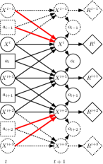
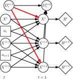
Figure 2: Left: A 2-agent sub-problem within 4-agent FFG. Right: the corresponding IASP.

The overall approach that we take is to divide the problem into sub-problems (defined here), compute overestimations of the achievable value for each of these sub-problems (discussed in Section 4) and combine those into a global upper bound (Section 5).

3.1 Sub-Problems (SPs)

The notion of a sub-problem generalizes the concept of a local-form model (LFM) Oliehoek12AAAI_IBA to multiple agents and reward components. We give a relatively concise description of this formalization, for more details, please see Oliehoek12AAAI_IBA .

Definition 0.

A sub-problem (SP) $\mathcal{M}_{c}$ of a factored Dec-POMDP $\mathcal{M}$ is a tuple $\mathcal{M}_{c}=\langle\mathcal{M},\mathcal{D}^{\prime},\mathcal{X}^{\prime},\mathcal{R}^{\prime}\rangle$, where $\mathcal{D}^{\prime}\subset\mathcal{D},\mathcal{X}^{\prime}\subset\mathcal{X},\mathcal{R}^{\prime}\subset\mathcal{R}$ denote subsets of agents, state factors and local reward functions.

An SP inherits many features from $\mathcal{M}$: we can define local states ${x}_{c}\in\bigotimes_{X\in\mathcal{X}^{\prime}}$ and the subsets $\mathcal{D}^{\prime},\mathcal{X}^{\prime},\mathcal{R}^{\prime}$ induce local joint actions ${\mathcal{A}}_{c}=\bigotimes_{i\in\mathcal{D}^{\prime}}{\mathcal{A}}_{i}$, observations ${\mathcal{O}}_{c}=\bigotimes_{i\in\mathcal{D}^{\prime}}{\mathcal{O}}_{i}$, and rewards

$${R}_{c}({x}_{c},{a}_{c},{x}_{c}^{\prime})\operatorname{\triangleq}\sum_{l\in\mathcal{R}^{\prime}}{R}^{l}({x}_{l},{{a}_{l}},{x}_{l}^{\prime}).$$ (1)

However, this is generally not enough to end up with a fully specified, but smaller, factored Dec-POMDP. This is illustrated in Fig. 2(left), which shows the 2DBN for a sub-problem of FFG involving two agents and three houses (dependence of observations ${{o}_{i}}$ on actions ${{a}_{i}}$ is not displayed). The figure shows that state factors $X\in\mathcal{X}^{\prime}$ (in this case ${X}^{i}$ and ${X}^{i+2}$) can be the target of arrows pointing into the sub-problem from the non-modeled (dashed) part. We refer to such state factors as non-locally affected factors (NLAFs) and denote them ${{xn}_{c}^{k}}$, where $c$ indexes the SP and $k$ indexes the factor. The other state factors in $\mathcal{X}^{\prime}$ are referred to as only-locally affected factors (OLAFs) ${{xl}_{c}^{k}}$. The figure clearly shows that the transition probabilities are not well-defined since the NLAFs depend on the sources of the highlighted influence links. We refer to these sources as influence sources ${u}_{c}^{t+1}=\left\langle{y}_{u}^{t},{{a}_{u}^{t}}\right\rangle$ (in this case ${y}_{u}^{t}=\left\langle{X}^{i-1},{X}^{i+3}\right\rangle$ and ${{a}_{u}^{t}}=\left\langle{{a}_{i-1}^{t}},{{a}_{i+2}^{t}}\right\rangle$). This means that an SP $c$ has an underspecified transition model: $T_{c}({{x}_{c}^{t+1}}|{{x}_{c}^{t}},{{a}_{c}^{t}},{u}_{c}^{t+1})$.

3.2 Structural Assumptions

In the most general form, the observation and reward model could also be underspecified. In order to simplify the exposition, we make two assumptions on the structure of an SP:

1. For all included agents $i\in\mathcal{D}^{\prime}$, the state factors that can influence its observations (i.e., ancestors of ${{o}_{i}}$ in the 2DBN) are included in $\mathcal{M}_{c}$.

2. For all included reward components ${R}^{l}\in\mathcal{R}^{\prime}$, the state factors and actions that influence ${R}^{l}$ are included in $\mathcal{M}_{c}$.

That is, we assume that SPs exhibit generalized forms of observation independence,

$$O_{c}({o}_{c}|{a}_{c},{x}_{c}^{\prime})\operatorname{\triangleq}\Pr({o}_{c}|{a}_{c},{x}_{c}^{\prime})=\Pr({o}_{c}|{a},s^{\prime}),$$

and reward independence (cf. (1)). These are more general notions of observation and reward independence than used in previous work on TOI-Dec-MDPs Becker03AAMAS and ND-POMDPs Nair05AAAI , since we allow overlap on state factors that can be influenced by the agents themselves.

Crucially, however, we do not assume any form of transition independence (for instance, the sets $\mathcal{X}^{\prime}$ of SPs can overlap), nor do we assume any of the transition-decoupling (i.e., TD-POMDP Witwicki10ICAPS ) restrictions. That is, we neither restrict which node types can affect ‘private’ nodes; nor do we disallow concurrent interaction effects on ‘mutually modeled’ nodes.

This means that assumptions 1 and 2 (above) that we do make are without loss of generality: it is possible to make any Dec-POMDP problem satisfy them by introducing additional (dummy) state factors.

3.3 Influence-Augmented SPs

An LFM can be transformed into a so-called influence-augmented local model, which captures the influence of the policies and parts of the environment that are not modeled in the local model Oliehoek12AAAI_IBA . Here we extend this approach to SPs, thus leading to influence-augmented sub-problems (IASPs).

Intuitively, the construction of an IASP consists of two steps: 1) capturing the influence of the non-modeled parts of the problem (given ${\pi}_{\neq{c}}$ the policies of non-modeled agents) in an incoming influence point ${I}_{\rightarrow c}({\pi}_{-c})$, and 2) using this ${I}_{\rightarrow c}$ to create a model with a transformed transition model $T_{{I}_{\rightarrow c}}$ and no further dependence on the external problem.

Step (1) can be done as follows: an incoming influence point can be specified as an incoming influence ${I}_{\rightarrow c}^{t}$ for each stage: ${I}_{\rightarrow c}=\left({I}_{\rightarrow c}^{1},\dots,{I}_{\rightarrow c}^{h}\right)$. Each such ${I}_{\rightarrow c}^{t+1}$ corresponds to the influence that the SP experiences at stage $t+1$, and thus specifies the conditional probability distribution of the influence sources ${u}_{c}^{t+1}=\left\langle{y}_{u}^{t},{{a}_{u}^{t}}\right\rangle$. That is, assuming that the influencing agents use deterministic policies ${\pi}_{u}=\langle{\pi}_{i}\rangle_{i\in u}$ that map observation histories to actions, ${I}_{\rightarrow c}^{t+1}$ is the conditional probability distribution given by

$$I({u}_{c}^{t+1}\,|\,{D}_{c}^{t+1})=\\ \sum_{{\@vec{o}{}}_{u}^{\;t}}\boldsymbol{1}_{\{{{a}_{u}^{t}}={\pi}_{u}({\@vec{o}{}}_{u}^{\;t})\}}\Pr({y}_{u}^{t},{\@vec{o}{}}_{u}^{\;t}|{D}_{c}^{t+1},{b^{0}},{\pi}_{\neq{c}}),$$

where $\boldsymbol{1}_{\{\cdot\}}$ is the Kronecker Delta function, and ${D}_{c}^{t+1}$ the d-separating set for ${I}_{\rightarrow c}^{t+1}$: the history of a subset of all the modeled variables that d-separates the modeled variables from the non-modeled ones.

Step (2) involves replacing the CPTs for all the NLAFs by the CPTs induced by ${I}_{\rightarrow c}$.

Definition 0.

Let ${{xn}_{c}^{k,t+1}}$ be an NLAF (with index $k$), and ${u}_{c}^{t+1}$ (the instantiation of) the corresponding influence sources. Given the influence ${I}_{\rightarrow c}^{t+1}({\pi}_{\neq{c}})$, and its d-separating set ${D}_{i}^{t+1}$, we define the induced CPT for ${{xn}_{c}^{k,t+1}}$ as the CPT that specifies probabilities:

$$p_{{I}_{\rightarrow c}^{t+1}}({{xn}_{c}^{k,t+1}}|{{x}_{c}^{t}},{D}_{c}^{t+1},{{a}_{c}^{t}})=\\ \sum_{{u}_{c}^{t+1}=\left\langle{y}_{u}^{t},{{a}_{u}^{t}}\right\rangle}\Pr({{xn}_{c}^{k,t+1}}|{{x}_{c}^{t}},{{a}_{c}^{t}},{u}_{c}^{t+1})I({u}_{c}^{t+1}|{D}_{c}^{t+1}).$$ (2)

Finally, we can define the IASP.

Definition 0.

An influence-augmented SP (IASP) $\mathcal{M}_{c}^{IA}$ $=\langle\mathcal{M}_{c},{I}_{\rightarrow c}\rangle$ for an SP $\mathcal{M}_{c}=\langle\mathcal{M},\mathcal{D}^{\prime},\mathcal{X}^{\prime},\mathcal{R}^{\prime}\rangle$ is a factored Dec-POMDP with the following components:

• The agents (implying the actions and observations) from the respective subproblem participate: $\bar{\mathcal{D}}=\mathcal{D}^{\prime}$.

• The set of state factors is $\bar{\mathcal{X}}=\mathcal{X}^{\prime}\cup\{{D}_{c}\}$ such that states ${\bar{{x}}}_{c}^{t}=\langle{{x}_{c}^{t}},{D}_{c}^{t+1}\rangle$ specify a local state of the SP, as well as the d-separating set ${D}_{i}^{t+1}$ for the next-stage influences.

• Transitions are specified as follows: For all OLAFs ${{x}_{c}^{k}{}}$ we take the CPTs from the factored Dec-POMDP $\mathcal{M}$, but for all NLAFs we take the induced CPTs, leading to an influence-augmented transition model which is the product of CPTs of OLAFs and NLAFS:

  $$\bar{T}_{{I}_{\rightarrow c}}({{x}_{c}^{t+1}}|\langle{{x}_{c}^{t}},{D}_{c}^{t+1}\rangle,{{a}_{c}^{t}})=\Pr({{xl}_{c}^{t+1}}|{{x}_{c}^{t}},{{a}_{c}^{t}})\\ \sum_{{u}_{c}^{t+1}=\left\langle{y}_{u}^{t},{{a}_{u}^{t}}\right\rangle}\Pr({{xn}_{c}^{t+1}}|{{x}_{c}^{t}},{{a}_{c}^{t}},{u}_{c}^{t+1})I({u}_{c}^{t+1}|{D}_{c}^{t+1}).$$ (3)

  (Note that ${{x}_{c}^{t}},{{a}_{c}^{t}},{{x}_{c}^{t+1}}$ and ${D}_{c}^{t+1}$ together uniquely specify ${D}_{c}^{t+2}$).

• The observation model $\bar{O}$ follows directly from $O$ (from $\mathcal{M}$).

• The reward is identical to that of the SP: $\bar{\mathcal{R}}=\mathcal{R}^{\prime}$.

Fig. 2(right) illustrates the IASP for FFG. It shows how the d-separating set acts as a parent for all NLAFs, thus replacing the dependence on the external part of the problem.

We write ${V}_{c}(\pi)$ for the value that would be realized for the reward components modeled in sub-problem $c$, under a given joint policy $\pi$:

$${V}_{c}(\pi)\operatorname{\triangleq}\mathbf{E}\left[\sum_{t=0}^{h-1}{R}_{c}^{t}(s,{a},s^{\prime})\mid{b^{0}},\pi\right].$$

As one can derive, given the policies of other agents ${\pi}_{\neq{c}}$, $V_{c}({I}_{\rightarrow c}({\pi}_{\neq{c}}))$, the value of the optimal solution of an IASP constructed for the influence corresponding to ${\pi}_{\neq{c}}$, is equal to the best-response value:

$$V_{c}^{BR}({\pi}_{\neq{c}})\operatorname{\triangleq}\max_{{\pi}_{c}}{V}_{c}({\pi}_{c},{\pi}_{\neq{c}})=V_{c}({I}_{\rightarrow c}({\pi}_{\neq{c}})).$$ (4)

This extends the result in Oliehoek12AAAI_IBA to multiagent SPs.

4 Local Upper Bounds

In this section we present our main technical contribution: the machinery to compute influence-optimistic upper bounds (IO-UBs) for the value of sub-problems. In order to properly define this class of upper bound, we first define the locally-optimal value:

Definition 0.

The locally-optimal value for an SP $c$,

$$V_{c}^{LO}\operatorname{\triangleq}\max_{{\pi}_{\neq{c}}}V_{c}^{BR}({\pi}_{\neq{c}})=\max_{{\pi}_{\neq{c}}}V_{c}({I}_{\rightarrow c}({\pi}_{\neq{c}})),$$ (5)

is the local value (considering only the rewards ${R}_{c}$) that can be achieved when all agents use a policy selected to optimize this local value. We will denote the maximizing argument by ${\pi}_{\neq{c}}^{LO}$.

Note that $V_{c}^{LO}\geq V_{c}(\pi^{*})$—the value for the rewards ${R}_{c}$ under the optimal joint policy $\pi^{*}$—since $\pi^{*}$ optimizes the sum of all local reward functions: it might be optimal to sacrifice some reward ${R}_{c}$ if it is made up by higher rewards outside of the sub-problem.

$V_{c}^{LO}$ expresses the maximal value achievable under a feasible incoming influence point; i.e., it is optimistic about the influence, but maintains that the influence is feasible. Computing this value can be difficult, since computing influences and subsequently constructing and optimally solving an IASP can be very expensive in general. However, it turns out computing upper bounds to $V_{c}^{LO}$ can be done more efficiently, as discussed in Section 4.4.

The IO-UBs that we propose in the remainder of this section upper-bound $V_{c}^{LO}$ by relaxing the requirement of the incoming influence being feasible, thus allowing for more efficient computation. We present three approaches that each overestimate the value by being optimistic with respect to the assumed influence, but that differ in the additional assumptions that they make.

4.1 A Q-MMDP Approach

The first approach we consider is called influence-optimistic Q-MMDP (IO-Q-MMDP). Like all the heuristics we introduce, it assumes that the considered SP will receive the most optimistic (possibly infeasible) influence. In addition, it assumes that the SP is fully observable such that it reduces to a local multiagent MDP (MMDP) Boutilier96AAAI . In other words, this approach resembles Q-MMDP Szer05UAI_MAA ; Oliehoek08JAIR , but is applied to an SP, and performs an influence-optimistic estimation of value. IO-Q-MMDP makes, in addition to influence optimism, another overestimation due to its assumption of full observability. While this negatively affects the tightness of the upper bound, it has as the advantage that its computational complexity is relatively low.

Formally, we can describe IO-Q-MMDP as follows. In the first phase, we apply dynamic programming to compute the action-values for all local states:

$$\negmedspace\negmedspace\negmedspace\negmedspace Q({{x}_{c}^{t}},{{a}_{c}^{t}})=\max_{{u}_{c}^{t+1}}\sum_{{{x}_{c}^{t+1}}}\Pr({{xl}_{c}^{t+1}}|{{x}_{c}^{t}},{{a}_{c}^{t}})\Pr({{xn}_{c}^{t+1}}|{{x}_{c}^{t}},{{a}_{c}^{t}},{u}_{c}^{t+1})\\ \Big{[}{R}_{c}({{x}_{c}^{t}},{{a}_{c}^{t}},{{x}_{c}^{t+1}})+\max_{{{a}_{c}^{t+1}}}Q({{x}_{c}^{t+1}},{{a}_{c}^{t+1}})\Big{]}.$$ (6)

Comparing this equation to (3), it is clear that this equation is optimistic with respect to the influence: it selects the sources ${u}_{c}^{t+1}$ in order to select the most beneficial transition probabilities. In the second phase, we use these values to compute an upper bound:

$${\hat{V}}_{c}^{M}\operatorname{\triangleq}\max_{{{a}_{c}}}\sum_{{{x}_{c}}}{b^{0}}({{x}_{c}})Q({{x}_{c}},{{a}_{c}}).$$

This procedure is guaranteed to yield an upper bound to the locally-optimal value for the SP.

Theorem 6.

IO-Q-MMDP yields an upper bound to the locally-optimal value: $V_{c}^{LO}\leq{\hat{V}}_{c}^{M}$.

Proof.

An inductive argument easily establishes that, due to the maximization it performs, (6) is at least as great as the Q-MMDP value (for all ${D}_{c}^{t+1}$) of any feasible influence, given by:

$$Q_{c}^{\mathit{MMDP}}(\langle{{x}_{c}^{t}},{D}_{c}^{t+1}\rangle,{{a}_{c}^{t}})=\sum_{{{x}_{c}^{t+1}}}\bar{T}_{{I}_{\rightarrow c}}({{x}_{c}^{t+1}}|\langle{{x}_{c}^{t}},{D}_{c}^{t+1}\rangle,{{a}_{c}^{t}})\\ \Big{[}{R}_{c}({{x}_{c}^{t}},{{a}_{c}^{t}},{{x}_{c}^{t+1}})+\max_{{{a}_{c}^{t+1}}}Q(\langle{{x}_{c}^{t+1}},{D}_{c}^{t+2}\rangle,{{a}_{c}^{t+1}})\Big{]}.$$ (7)

Therefore the value computed in (6) is at least as great as the Q-MMDP value (7) induced by ${\pi}_{\neq{c}}^{LO}$ (the maximizing argument of (5)), for all ${{x}_{c}^{t}},{D}_{c}^{t+1},{{a}_{c}^{t}}$. This directly implies

$${\hat{V}}_{c}^{M}\geq V_{c}^{\mathit{MMDP}}({I}_{\rightarrow c}({\pi}_{\neq{c}}^{LO})),$$

Moreover, it is well known that, for any Dec-POMDP, the Q-MMDP value is an upper bound to its value Szer05UAI_MAA , such that

$$V_{c}^{\mathit{MMDP}}({I}_{\rightarrow c}({\pi}_{\neq{c}}^{LO}))\geq V_{c}({I}_{\rightarrow c}({\pi}_{\neq{c}}^{LO})).$$

We can conclude that ${\hat{V}}_{c}^{M}$ is an upper bound to the Dec-POMDP value of the IASP induced by ${\pi}_{\neq{c}}^{LO}$:

$${\hat{V}}_{c}^{M}\geq V_{c}({I}_{\rightarrow c}({\pi}_{\neq{c}}^{LO}))=\max_{{\pi}_{\neq{c}}}V_{c}({I}_{\rightarrow c}({\pi}_{\neq{c}}))=V_{c}^{LO},$$

with the identities given by (5), thus proving the theorem.∎

The upshot of (6) is that there are no dependencies on d-separating sets and incoming influences anymore: the IO assumption effectively eliminates these dependencies. As a result, there is no need to actually construct the IASPs (that potentially have a very large-state-space) if all we are interested in is an upper bound.

4.2 A Q-MPOMDP Approach

The IO-Q-MMDP approach of the previous section introduces overestimations through influence-optimism as well as by assuming full observability. Here we tighten the upper bound by weakening the second assumption. In particular, we propose an upper bound based on the underlying multiagent POMDP (MPOMDP).

An MPOMDP Messias11NIPS24 ; Amato13MSDM is partially observable, but assumes that the agents can freely communicate their observations, such that the problem reduces to a special type of centralized model in which the decision maker (representing the entire team of agents) takes joint actions, and receives joint observations. As a result, the optimal value for an MPOMDP is analogous to that of a POMDP:

$$Q({{b}}^{t},{{{a}}^{t}})=R({{b}}^{t},{{{a}}^{t}})+\sum_{{{o}^{t+1}}}\Pr({{o}^{t+1}}|{{b}}^{t},{{{a}}^{t}})V({{b}}^{t+1}),$$ (8)

where ${{b}}^{t+1}$ is the joint belief resulting from performing Bayesian updating of ${{b}}^{t}$ given ${{{a}}^{t}}$ and ${{o}^{t+1}}$.

Using the value function of the MPOMDP solution as a heuristic (i.e., an upper bound) for the value function of a Dec-POMDP is a technique referred to as Q-MPOMDP Roth05AAMAS ; Oliehoek08JAIR . Here we combine this approach with optimistic assumptions on the influences, leading to influence-optimistic Q-MPOMDP (IO-Q-MPOMDP).

In case that the influence on an SP is fully specified, (8) can be readily applied to the IASP. However, we want to deal with the case where this influence is not specified. The basic, conceptually simple, idea is to move from the influence-optimistic MMDP-based upper bounding scheme from in Section 4.1 to one based on MPOMDPs. However, it presents a technical difficulty, since it is not directly obvious how to extend (6) to deal with partial observability. In particular, in the MPOMDP case as given by (8), the state ${{x}_{c}^{t}}$ is replaced by a belief over such local states and the influence sources ${u}_{c}^{t+1}$ affect the value by both manipulating the transition and observation probabilities, as well as the resulting beliefs.

To overcome these difficulties, we propose a formulation that is not directly based on (8), but that too makes use of ‘back-projected value vectors’. That is, it is possible to rewrite the optimal MPOMDP value function as:

$$Q({{b}}^{t},{{{a}}^{t}})={{{b}}^{t}}\cdot{r_{a}}+\gamma\sum_{{{o}^{t+1}}}\max_{\nu^{ao}\in\mathcal{V}^{ao}}{{{b}}^{t}}\cdot{\nu^{ao}},$$ (9)

where ${}\cdot{}$ denotes inner product and where $\nu^{ao}\in\mathcal{V}^{ao}$ are the back-projections of value vectors $\nu\in\mathcal{V}^{t+1}$:

$$\nu^{ao}({{s}^{t}})\operatorname{\triangleq}\sum_{{{s}^{t+1}}}O({{o}^{t+1}}|{{{a}}^{t}},{{s}^{t+1}})T({{s}^{t+1}}|{{s}^{t}}{{{a}}^{t}})\nu({{s}^{t+1}}).\negthickspace$$ (10)

(Please see, e.g., Spaan12RLBook ; Shani13JAAMAS for more details.)

The key insight that enables carrying influence-opti-mism to the MPOMDP case is that this back-projected form (10) does allow us to take the maximum with respect to unspecified influences. That is, we define the influence-optimistic back-projection as:

$$\nu_{IO}^{ao}({{x}_{c}^{t}})\operatorname{\triangleq}\max_{{u}_{c}^{t+1}}\sum_{{{x}_{c}^{t+1}}}O({{o}_{c}^{t+1}}|{{a}_{c}},{{x}_{c}^{t+1}})\\ \Pr({{xn}_{c}^{t+1}}|{{x}_{c}^{t}},{{a}_{c}},{u}_{c}^{t+1})\Pr({{xl}_{c}^{t+1}}|{{x}_{c}^{t}},{{a}_{c}})\nu_{IO}({{x}_{c}^{t+1}}).$$ (11)

Since this equation does not depend in any way on the d-separating sets and influence, we can completely avoid generating large IASPs. As for implementation, many POMDP solution methods Cassandra97UAI ; Kaelbling98AI are based on such back-projections and therefore can be easily modified; all that is required is to substitute these the back-projections by their modified form (11). When combined with an exact POMDP solver, such influence-optimistic back-ups will lead to an upper bound ${\hat{V}}_{c}^{P}$, to which we refer as IO-Q-MPOMDP, on the locally-optimal value.

To formally prove this claim, we will need to discriminate a few different types of value, and associated constructs. Let us define:

• ${\bar{{{b}}}}_{{I}_{\rightarrow c}}^{t}(\langle{{x}_{c}^{t}},{D}_{c}^{t+1}\rangle)$, an MPOMDP belief for the IASP induced by an arbitrary influence ${I}_{\rightarrow c}$,

• $V_{{I}_{\rightarrow c}}^{P}$, the optimal value function when the IASP is solved as an MPOMDP, such that $V_{{I}_{\rightarrow c}}^{P}({\bar{{{b}}}}_{{I}_{\rightarrow c}}^{t})$ is the value of ${\bar{{{b}}}}_{{I}_{\rightarrow c}}^{t}$ and $\mathit{V}_{c}^{MPOMDP}({I}_{\rightarrow c})\operatorname{\triangleq}V_{{I}_{\rightarrow c}}^{P}({\bar{{{b}}}}_{{I}_{\rightarrow c}}^{0})$. $V_{{I}_{\rightarrow c}}^{P}$ is represented using vectors $\nu\in\mathcal{V}$.

• ${\bar{{{b}}}}_{IO}^{t}({{x}_{c}^{t}})$, an arbitrary distribution over ${{x}_{c}^{t}}$ that can be thought of as the MPOMDP belief for the ‘influence optimistic SP’.

• $V_{IO,c}^{P}$, the value function computed by an (exact) influence-optimistic MPOMDP method, that assigns a value $V_{IO,c}^{P}({\bar{{{b}}}}_{IO}^{t})$ to any ${\bar{{{b}}}}_{IO}^{t}$. $V_{IO,c}^{P}$ is represented using vectors $\nu_{IO}\in\mathcal{V}_{IO}$. The IO-Q-MPOMDP upper bound is defined by plugging in the true initial state distribution ${b^{0}}$, restricted to factors in $c$: ${\hat{V}}_{c}^{P}\operatorname{\triangleq}V_{c}^{P}({\bar{{{b}}}}_{IO}^{0})$.

First we establish a relation between the different vectors representing $V_{{I}_{\rightarrow c}}^{P}$ and $V_{IO,c}^{P}$.

Lemma 0.

Let ${\pi}_{c}^{t:h-1}$ be a $(h-t)$-steps-to-go policy. Let $\nu\in\mathcal{V}$ and $\nu_{IO}\in\mathcal{V}_{IO}$ be the vectors induced by ${\pi}_{c}^{t:h-1}$ under regular MPOMDP back-projections (for some ${I}_{\rightarrow c}$), and under IO back-projections respectively. Then

$$\forall_{{{x}_{c}^{t}}}\qquad\max_{{D}_{c}^{t+1}}\nu(\langle{{x}_{c}^{t}},{D}_{c}^{t+1}\rangle)\leq\nu_{IO}({{x}_{c}^{t}}).$$

Proof.

The proof is listed in Appendix A.∎

This lemma provides a strong result on the relation of values computed under regular MPOMDP backups versus influence-optimistic ones. It allows us to establish the following theorem:

Theorem 8.

For an SP $c$, for all ${I}_{\rightarrow c}$,

$$\forall_{{\bar{{{b}}}}_{{I}_{\rightarrow c}}^{t}}\qquad V_{{I}_{\rightarrow c}}^{P}({\bar{{{b}}}}_{{I}_{\rightarrow c}}^{t})\leq V_{IO,c}^{P}({\bar{{{b}}}}_{IO}^{t}),$$

provided that ${\bar{{{b}}}}_{IO}^{t}$ concides with the marginals of ${\bar{{{b}}}}_{{I}_{\rightarrow c}}^{t}$:

$$\text{(A1)}\hskip 10.00002pt\forall_{{{x}_{c}^{t}}}\;\sum_{{D}_{c}^{t+1}}{\bar{{{b}}}}_{{I}_{\rightarrow c}}^{t}(\langle{{x}_{c}^{t}},{D}_{c}^{t+1}\rangle)={\bar{{{b}}}}_{IO}^{t}({{x}_{c}^{t}}).$$

Proof.

We start with the left hand side:

$$\hskip-30.00005ptV_{{I}_{\rightarrow c}}^{P}({\bar{{{b}}}}_{c}^{t})=\max_{\nu\in\mathcal{V}}{{\bar{{{b}}}}_{{I}_{\rightarrow c}}^{t}}\cdot{\nu}$$

$$= \max_{\nu\in\mathcal{V}}\sum_{\langle{{x}_{c}^{t}},{D}_{c}^{t+1}\rangle}{\bar{{{b}}}}_{{I}_{\rightarrow c}}^{t}(\langle{{x}_{c}^{t}},{D}_{c}^{t+1}\rangle)\nu(\langle{{x}_{c}^{t}},{D}_{c}^{t+1}\rangle)$$

$$\leq \max_{\nu\in\mathcal{V}}\sum_{{{x}_{c}^{t}}}\sum_{{D}_{c}^{t+1}}{\bar{{{b}}}}_{{I}_{\rightarrow c}}^{t}(\langle{{x}_{c}^{t}},{D}_{c}^{t+1}\rangle)\max_{{D}_{c}^{t+1}}\nu(\langle{{x}_{c}^{t}},{D}_{c}^{t+1}\rangle)$$

$$\text{\{A1\}}= \max_{\nu\in\mathcal{V}}\sum_{{{x}_{c}^{t}}}{\bar{{{b}}}}_{IO}^{t}({{x}_{c}^{t}})\max_{{D}_{c}^{t+1}}\nu(\langle{{x}_{c}^{t}},{D}_{c}^{t+1}\rangle)$$

{Lemma 7}

$$\leq \max_{\nu_{IO}\in\mathcal{V}_{IO}}\sum_{{{x}_{c}^{t}}}{\bar{{{b}}}}_{IO}^{t}({{x}_{c}^{t}})\nu_{IO}({{x}_{c}^{t}})$$

$$= \max_{\nu_{IO}\in\mathcal{V}_{IO}}{{\bar{{{b}}}}_{IO}^{t}}\cdot{\nu_{IO}}$$

$$= \,V_{IO,c}^{P}({\bar{{{b}}}}_{IO}^{t}),$$

thus proving the theorem.∎

Corollary 0.

IO-Q-MPOMDP yields an upper bound to the locally-optimal value: $V_{c}^{LO}\leq{\hat{V}}_{c}^{P}$.

Proof.

The initial beliefs are defined such that the above condition (A1) holds. That is:

$$\sum_{{D}_{c}^{t+1}}{\bar{{{b}}}}_{{I}_{\rightarrow c}}^{0}(\langle{{x}_{c}^{0}},{D}_{c}^{1}=\emptyset\rangle)={\bar{{{b}}}}_{IO}^{0}({{x}_{c}^{t}})={b^{0}}({{x}_{c}^{t}}).$$

Therefore, application of Theorem 8 to the initial belief yields:

$$\forall_{{I}_{\rightarrow c}}\;{\hat{V}}_{c}^{P}\operatorname{\triangleq}V_{IO,c}^{P}({\bar{{{b}}}}_{IO}^{0})\geq V_{{I}_{\rightarrow c}}^{P}({\bar{{{b}}}}_{{I}_{\rightarrow c}}^{0})\operatorname{\triangleq}V_{c}^{\mathit{MPOMDP}}({I}_{\rightarrow c})$$

It is well-known that the MPOMDP value is an upper bound to the Dec-POMDP value Oliehoek08JAIR , such that

$$V_{c}^{\mathit{MPOMDP}}({I}_{\rightarrow c}({\pi}_{\neq{c}}^{LO}))\geq V_{c}({I}_{\rightarrow c}({\pi}_{\neq{c}}^{LO})),$$

and we can immediately conclude that

$${\hat{V}}_{c}^{P}\geq V_{c}({I}_{\rightarrow c}({\pi}_{\neq{c}}^{LO}))=\max_{{\pi}_{\neq{c}}}V_{c}({I}_{\rightarrow c}({\pi}_{\neq{c}}))=V_{c}^{LO},$$

with the identities given by (5), proving the result.∎

4.3 A Dec-POMDP Approach

The previous approaches compute upper bounds by, apart from the IO assumption, additionally making optimistic assumptions on observability or communication capabilities. Here we present a general method for computing Dec-POMDP-based upper bounds that, other than the optimistic assumptions about neighboring SPs, make no additional assumptions and thus provide the tightest bounds out of the three that we propose. This approach builds on the recent insight MacDermed13NIPS26 ; Dibangoye13IJCAI ; Oliehoek13JAIR that a Dec-POMDP can be converted to a special case of POMDP (for an overview of this reduction, see Oliehoek14IASTR ); we can thereby leverage the influence-optimistic back-projection (11) to compute an IO-UB that we refer to as IO-Q-Dec-POMDP.

As in the previous two sub-sections, we will leverage optimism with respect to an influence-augmented model that we will never need to construct. In particular, as explained in Section 3 we can convert an SP $\mathcal{M}_{c}$ to an IASP $\mathcal{M}_{c}^{IA}$ given an influence ${I}_{\rightarrow c}$. Since such an IASP is a Dec-POMDP, we can convert it to a special case of a POMDP:

Definition 0.

A plan-time influence-augmented sub-problem, $\mathcal{M}_{c}^{\text{PT-IA}}$, is a tuple $\mathcal{M}_{c}^{\text{PT-IA}}(\mathcal{M}_{c},{I}_{\rightarrow c})=\left\langle{\check{\mathcal{S}}},{\check{{\mathcal{A}}}},{\check{T}}_{{I}_{\rightarrow c}},{\check{R}},{\check{{\mathcal{O}}}},{\check{O}},{\check{h}},{\check{{b^{0}}}}\right\rangle$, where:

• ${\check{\mathcal{S}}}$ is the set of states ${{\check{s}}}^{t}=\left\langle{\bar{{x}}}_{c}^{t},{\@vec{o}{}}_{c}^{\;t}\right\rangle=\left\langle{{x}_{c}^{t}},{D}_{c}^{t+1},{\@vec{o}{}}_{c}^{\;t}\right\rangle$.

• ${\check{{\mathcal{A}}}}$ is the set of actions, each ${{\check{{{a}}}}}^{t}$ corresponds to a local joint decision rule ${\delta}_{c}^{t}$ in the SP.

• ${\check{T}}_{{I}_{\rightarrow c}}({{\check{s}}}^{t+1}|{{\check{s}}}^{t},{{\check{{{a}}}}}^{t})$ is the transition function defined below.

• ${\check{R}}({{\check{s}}}^{t},{{\check{{{a}}}}}^{t})={R}_{c}({{x}_{c}^{t}},{\delta}_{c}^{t}({\@vec{o}{}}_{c}^{\;t}))$.

• ${\check{{\mathcal{O}}}}=\left\{\mathit{NULL}\right\}$.

• ${\check{O}}$ specifies that observation $\mathit{NULL}$ is received with probability 1 (irrespective of the state and action).

• The horizon is not modified: ${\check{h}}=h$.

• ${\check{{b^{0}}}}$ is the initial state distribution. Since there is only one $\@vec{o}{}{}^{\;0}$ (i.e., the empty joint observation history).

The transition function specifies:

$${\check{T}}_{{I}_{\rightarrow c}}(\left\langle{{x}_{c}^{t+1}},{D}_{c}^{t+2},{\@vec{o}{}}_{c}^{\;t+1}\right\rangle|\left\langle{{x}_{c}^{t}},{D}_{c}^{t+1},{\@vec{o}{}}_{c}^{\;t}\right\rangle,{\delta}_{c}^{t})\\ \operatorname{\triangleq}\bar{T}_{{I}_{\rightarrow c}}({{x}_{c}^{t+1}}|\langle{{x}_{c}^{t}},{D}_{c}^{t+1}\rangle,{\delta}_{c}^{t}({\@vec{o}{}}_{c}^{\;t}))\bar{O}({{o}_{c}^{t+1}}|{\delta}_{c}^{t}({\@vec{o}{}}_{c}^{\;t}),{{x}_{c}^{t+1}})$$

if ${\@vec{o}{}}_{c}^{\;t+1}=\left({\@vec{o}{}}_{c}^{\;t},{{o}_{c}^{t+1}}\right)$ and 0 otherwise. In this equation $\bar{T}_{{I}_{\rightarrow c}},\bar{O}$ are given by the IASP (cf. Section 3).

This reduction shows that it is possible to compute $V_{c}^{*}({I}_{\rightarrow c}({\pi}_{\neq{c}}))$, the optimal value for an SP given an influence point ${I}_{\rightarrow c}$, but the formulation is subject to the same computational burden as solving a regular IASP: constructing it is complex due to the inference that needs to be performed to compute ${I}_{\rightarrow c}$, and subsequently solving the IASP is complex due to the large number of augmented states ${{\check{s}}}^{t}=\left\langle{{x}_{c}^{t}},{D}_{c}^{t+1},{\@vec{o}{}}_{c}^{\;t}\right\rangle$.

Fortunately, here too we can compute an upper bound to any feasible incoming influence, and thus to $V_{c}^{LO}$, by using optimistic backup operations with respect to an underspecified model, to which we refer as simply plan-time SP:

Definition 0.

We define the plan-time sub-problem $\mathcal{M}_{c}^{\text{PT}}$ as an under-specified POMDP $\mathcal{M}_{c}^{\text{PT}}(\mathcal{M}_{c},\cdot)=\left\langle{\check{\mathcal{S}}},{\check{{\mathcal{A}}}},{\check{T}}_{(\cdot)},{\check{R}},{\check{{\mathcal{O}}}},{\check{O}},{\check{h}},{\check{{b^{0}}}}\right\rangle$ with

• states of the form ${{\check{s}}}^{t}=\left\langle{{x}_{c}^{t}},{\@vec{o}{}}_{c}^{\;t}\right\rangle$,

• an underspecified transition model

  $${\check{T_{(\cdot)}}}({{\check{s}}}^{t+1}|{{\check{s}}}^{t},{{\check{{{a}}}}}^{t})\operatorname{\triangleq}\\ T_{c}({{x}_{c}^{t+1}}|{{x}_{c}^{t}},{\delta}_{c}^{t}({\@vec{o}{}}_{c}^{\;t}),{u}_{c}^{t+1})O_{c}({{o}_{c}^{t+1}}|{\delta}_{c}^{t}({\@vec{o}{}}_{c}^{\;t}),{{x}_{c}^{t+1}}),$$

• and ${\check{{\mathcal{A}}}},{\check{R}},{\check{{\mathcal{O}}}},{\check{O}},{\check{h}},{\check{{b^{0}}}}$ as above.

Since this model is a special case of a POMDP, the theory developed in Section 4.2 applies: we can maintain a plan-time sufficient statistic ${\sigma}^{c,t}$ (essentially the ‘belief’ ${\check{b}}$ over augmented states ${{\check{s}}}^{t}=\left\langle{{x}_{c}^{t}},{\@vec{o}{}}_{c}^{\;t}\right\rangle$) and we can write down the value function using (9). Most importantly, the IO back-projection (11) also applies, which means that (similar to the MPOMDP case) we can avoid ever constructing the full PT-IASP. The IO back-projection in this case translates to:

$$\nu_{IO}^{{\delta}_{c}^{t}}({{x}_{c}^{t}},{\@vec{o}{}}_{c}^{\;t})\operatorname{\triangleq}\max_{{u}_{c}^{t+1}}\sum_{{{x}_{c}^{t+1}}}\Pr({{o}_{c}^{t+1}}|{\delta}_{c}^{t}({\@vec{o}{}}_{c}^{\;t}),{{x}_{c}^{t+1}})\\ \Pr({{xn}_{c}^{t+1}}|{{x}_{c}^{t}},{\delta}_{c}^{t}({\@vec{o}{}}_{c}^{\;t}),{u}_{c}^{t+1})\Pr({{xl}_{c}^{t+1}}|{{x}_{c}^{t}},{\delta}_{c}^{t}({\@vec{o}{}}_{c}^{\;t}))\\ \nu_{IO}({{x}_{c}^{t+1}},{\@vec{o}{}}_{c}^{\;t+1}).$$ (12)

Here, we omitted the superscript for the $\mathit{NULL}$ observation. Also, note that $O({{o}_{i}^{t+1}}|{{a}_{i}^{t}},{{x}_{i}^{t+1}})$ in (11) corresponds to the $\mathit{NULL}$ observation in the PT model, but since the observation histories are in the states, $\Pr({{o}_{c}^{t+1}}|{\delta}_{c}^{t}({\@vec{o}{}}_{c}^{\;t}),{{x}_{c}^{t+1}})$ comes out of the transition model.

Again, given this modified back-projection, the IO-Q-Dec-POMDP value ${\hat{V}}_{c}^{D}$ can be computed using any exact POMDP solution method that makes use of vector back-projections; all that is required is to substitute these the back projections by their modified form (12).

Corollary 0.

IO-Q-Dec-POMDP yields an upper bound to the locally-optimal value: $V_{c}^{LO}\leq{\hat{V}}_{c}^{D}$.

Proof.

Directly by applying ≘9 to $\mathcal{M}_{c}^{\text{PT}}.$∎

4.4 Computational Complexity

Due to the maximization in (6), (11) and (12), IO back-projections are more costly than regular (non-IO) back-projections. Here we analyze the computational complexity of the proposed algorithms relative to the regular, non-IO, backups.

We start by comparing IQ-Q-MMDP backup operation (6) to the regular MMDP backup for an SP that does not have incoming influences. For such an SP, the MMDP backup is given by

$$\negmedspace\negmedspace\negmedspace\negmedspace Q({{x}_{c}^{t}},{{a}_{c}^{t}})=\sum_{{{x}_{c}^{t+1}}}\Pr({{x}_{c}^{t+1}}|{{x}_{c}^{t}},{{a}_{c}^{t}})\\ \Big{[}{R}_{c}({{x}_{c}^{t}},{{a}_{c}^{t}},{{x}_{c}^{t+1}})+\max_{{{a}_{c}^{t+1}}}Q({{x}_{c}^{t+1}},{{a}_{c}^{t+1}})\Big{]}.$$ (13)

Comparing (6) and (13), we see two differences: 1) the transition probabilities can be written in one term since we do not need to discriminate NLAFs from OLAFs, and 2) there is no maximization over influence sources ${u}_{c}^{t+1}$. The first difference does not induce a change in computational cost, only in notation: in both cases the entire transition probability is given as the product of next-stage CPTs. The second difference does induce a change in computational cost: in (6), in order to select the maximum, the inner part of the right-hand side needs to be evaluated for each instantiation of the influence sources $\left|{u}_{c}^{t+1}\right|$. That is, the computational complexity of a Q-MMDP backup (for a particular $({{x}_{c}^{t}},{{a}_{c}^{t}})$-pair) is

$$O(\left|\mathcal{X}_{c}\right|\times\left|{{a}_{c}}\right|),$$

whereas the total computational cost of the IO-Q-MMDP backup is:

$$O(\left|{u}_{c}^{t+1}\right|\times\left|\mathcal{X}_{c}\right|\times\left|{{a}_{c}}\right|).$$

As such, the complexity of each backup is multiplied by the number of influence source instantiations $\left|{u}_{c}^{t+1}\right|$. This means that the overhead of IO-Q-MMDP relative to Q-MMDP is $O(\left|{u}_{c}^{t+1}\right|)$.

A similar comparison of the overhead of the IO-Q-MPOMDP back projection (11) with respect to the regular Q-MPOMDP back projection (10) leads to exactly the same relative overhead of $O(\left|{u}_{c}^{t+1}\right|)$. Since IO-Q-Dec-POMDP makes use of this last result, also in this case the relative overhead is $O(\left|{u}_{c}^{t+1}\right|)$.

Concluding, the computational complexity of the methods we proposed to compute IO-UBs is given by multiplying the computational complexity of the ‘underlying’ MMDP, MPOMDP or Dec-POMDP method with $\left|{u}_{c}^{t+1}\right|$. This means that the relative overhead, is equal for all methods. Since the amount of overhead is a linear function of $\left|{u}_{c}^{t+1}\right|$, it is problem dependent: more densely coupled problems will lead to a higher overhead, while very loosely coupled problems have a low overhead.

5 Global Upper Bounds

We next discuss how the methods to compute local upper bounds can be employed in order to compute a global upper bound for factored Dec-POMDPs.

The basic idea is to apply a non-overlapping decomposition $\mathcal{C}$ (i.e., a partitioning) of the reward functions $\left\{{R}^{l}\right\}$ of the original factored Dec-POMDP into SPs $c\in\mathcal{C}$, and to compute an IO upper bound $\hat{V}_{c}^{IO}$ for each (which can be any of the three IO-UBs proposed in Section 4). Our global influence-optimistic upper bound is then given by:

$$\hat{V}^{IO}\operatorname{\triangleq}\sum_{c\in\mathcal{C}}\hat{V}_{c}^{IO}.$$ (14)

Fig. 3 illustrates the construction of a global upper bound $\hat{V}$ for the 6-agent FFG, showing the original problem (top row) and two possible decompositions in SPs. The second row specifies a decomposition into two SPs, while the third row uses three SPs. The illustration clearly shows how (in this problem) a decomposition eliminates certain agents completely and replaces them with optimistic assumptions: E.g., in the second row, during the computation of $\hat{V}_{c}^{IO}$ for both SPs ($c=1,2$) the assumption is made that agent 3 will always fight fire in the SP under concern. Effectively we assume that agent 3 fights fire at both house 3 and house 4 simultaneously (and hence is represented by a superhero figure). Fig. 3 also illustrates that, due to the line structure of FFG, there are two types of SPs: ‘internal’ SPs which make optimistic assumptions on two sides, and ‘edge’ SPs that are optimistic at just one side.

Figure 3: Illustration of construction of a global upper bound for $6$-agent FFG using influence-optimistic upper bounds for sub-problems.

Finally, we formally prove the correctness of our proposed upper bounding scheme.

Theorem 13.

Let $\mathcal{C}$ be a partitioning of the reward function set $\mathcal{R}$ into sub-problems such that every ${R}^{l}$ is represented in one SP $c$, then the global IO-UB is in fact an upper bound to the optimal value $\hat{V}^{IO}\geq V(\pi^{*})$.

Proof.

Starting from the definition (14), we have

$$\hat{V}^{IO} \operatorname{\triangleq} \sum_{c\in\mathcal{C}}\hat{V}_{c}^{IO}\overset{\mathrm{\{Section\leavevmode\nobreak\ \ref{sec:local-upper-bounds}\}}}{\geq}\sum_{c\in\mathcal{C}}V_{c}^{LO}$$

$$\operatorname{\triangleq} \sum_{c\in\mathcal{C}}\max_{{\pi}_{\neq{c}}}V_{c}^{BR}({\pi}_{\neq{c}})$$

$$\operatorname{\triangleq} \sum_{c\in\mathcal{C}}\max_{{\pi}_{\neq{c}}}\max_{{\pi}_{c}}{V}_{c}({\pi}_{c},{\pi}_{\neq{c}})$$

$$\geq \max_{\pi}\sum_{c\in\mathcal{C}}{V}_{c}({\pi}_{c},{\pi}_{\neq{c}})\overset{\text{\{$\mathcal{C}$is a partition\}}}{=}V(\pi^{*})$$

thus proving the result. ∎

6 Empirical Evaluation

In order to test the potential impact of the proposed influence-optimistic upper bounds, we present numerical results in the context of a number of benchmark problems. In this evaluation, we focus on the (relative) values found by these heuristics, as we hope that these will spark a number of interesting ideas for further research (such as the notion of ‘influence strength’, its relation to approximability of factored Dec-POMDPs, and the key idea that reasonable bounds for very large problems may be possible). We do not thoroughly investigate timing results as the analysis of Section 4.4 indicates that relative timing results follow those of regular (non-IO) MMDP, MPOMDP and Dec-POMDP methods; see, e.g., Oliehoek08JAIR for a comparison of such timing results. However, in order to provide a overall idea of the run times, we do provide some indicative running times.

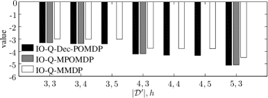
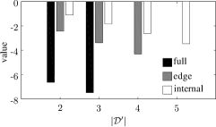
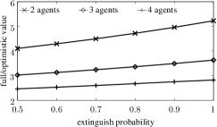
Figure 4: Left: Different IO-UBs on ‘edge’ FFG problems. Middle: IO-Q-Dec-POMDP upper bound on different types (internal, edge, full) of SPs. Right: The impact the ‘influence strength’.

6.1 Comparison of Different Bounds

The bounds that we propose are ordered in tightness, ${\hat{V}}_{c}^{D}\leq{\hat{V}}_{c}^{P}\leq{\hat{V}}_{c}^{M}$, similar to how regular (non-IO) Dec-POMDP, Q-MPOMDP, and Q-MMDP values relate Oliehoek08JAIR . To get an understanding of how these differences turn out in practice, Fig. 4(left) compares the different upper bounds introduced.

Although the approach described in the paper is general, in the numerical evaluation here we exploit the property that the optimistic influences are easily identified off-line, which allows for the construction of small ‘optimistic Dec-POMDPs’ (respectively MPOMDPs or MMDPs) without sacrificing in bound quality. E.g., in order to compute the local IQ-Q-Dec-POMDP upper bound for a 3-house FFG ‘edge’ SP, we define a regular 3-house Dec-POMDP where the transitions probabilities for the first house (say ${X}^{i}$ in Fig. 2) are modified to account for the optimistic assumption that another (superhero) agent fights fire there and that its neighbor is not burning (i.e., ${{a}_{i-1}}=right$ and ${X}^{i-1}=not\_burning$ in Fig. 2). The values ${\hat{V}}_{c}^{D}$ (resp. ${\hat{V}}_{c}^{P},{\hat{V}}_{c}^{M}$) are computed by running a state-of-the-art Dec-POMDP solver Oliehoek13JAIR (resp. incremental pruning Cassandra97UAI , plain dynamic programming) on such optimistically defined problems.

Fig. 4(left) shows the values for such ‘edge’ problems. Missing bars indicate time-outs (¿4h). As an indication of run time, the $|\mathcal{D}^{\prime}|=3,h=5$ problem took $2.21s$ for IO-Q-MMDP, and $995.28s$ for IO-Q-Dec-POMDP. The shown values indicate that ${\hat{V}}_{c}^{D},{\hat{V}}_{c}^{P}$ can be tighter than ${\hat{V}}_{c}^{M}$ in practice. In most cases, the difference between IO-Q-MPOMDP and IO-Q-Dec-POMDP is small, but these could become larger for longer horizons Oliehoek08JAIR . We performed the same analysis for the Aloha benchmark Oliehoek13AAMAS , and found very similar results.

We also compare the bounds found on the different types of SPs (internal and edge-cases, see Fig. 3) encountered in FFG ($h=4$). In addition, Fig. 4(middle) also includes—if computable within the allowed time—values of SPs that are ‘full’ problems (i.e., the regular optimal Dec-POMDP value for the full FFG instance with the indicated number of agents.) This makes clear that the optimistic assumption has quite some effect: being optimistic at one edge more than halves the optimal cost, and the IO assumption at both edges of the SP leads to another significant reduction of that cost. This is to be expected: the optimistic problems assume that there always will be another agent fighting fire at the house at an optimistic edge, while the full problem never has another agent at that same house. When also taking into account the transition probabilities—two agents at a house will completely extinguish a fire—it is clear that the IO assumption should have a high impact on the local value.

6.2 The Effect of Influence Strength

Fig. 4(middle) makes clear that the IO assumption in FFG is quite strong and leads to a significant over-estimation of the local value compared to the ‘full’ problem. We say that FFG has a high influence strength. In fact, this hints at a new dimension of the qualification of weak coupling Witwicki11AAMAS that takes into account the variance in NLAF probabilities (as a function of the change of value of the influence source) and their impact on the local value.

As a preliminary investigation of this concept, we devise a modification of FFG where the influence strength can be controlled. In particular, we parameterize the probability that a fire is extinguished completely when 2 agents visit the same house, which is set to 1 in the original problem definition. Lower values of this probability mean that optimistically assuming there is another agent at a house will lead to less advantage, and thus lower influence strength.

Fig. 4(right) shows the results of this experiment. It shows that there is a clear relation between the fire-extinguish probability when two agents fight fire at a house, and the ratio between the ‘regular’ (Dec-POMDP) value and optimistic value. It also shows that SPs with more agents are less affected: this makes sense since optimistic assumptions account for a smaller fraction of the achievable value. In other words, larger sub-problems give a tighter approximation.

6.3 Bounding Heuristic Methods

Here we investigate the ability to provide informative global upper bounds. While the previous analysis shows that the overestimation is quite significant at the true edges of the problem (where no agents exist), this is not necessarily informative of the overestimation at internal edges in decompositions of larger problems (where other agents do exist, even if not superheros). As such, besides investigating the upper bounding capability, the analysis here also provides a better understanding of such internal overestimations.

We use the tightest upper bound we could find by considering different SP partitions, with sizes ranging from $|\mathcal{D}|=2$–$5$, and investigate the guarantees that it can provide for transfer planning (TP) Oliehoek13AAMAS , which is one of the methods capable of providing solutions for large factored Dec-POMDPs. Since the method is a heuristic method that does not provide the exact value of the reported joint policy, the value of TP, $V^{\mathit{TP}}$, is determined using $10.000$ simulations of the found joint policy leading to accurate estimates. To put the results into context, we also show the value of a random policy. Finally, we show (second y-axis in Fig. 5) what we call the empirical approximation factor (EAF):

$$EAF=\max\{\frac{\hat{V}^{\mathit{IO}}}{V^{\mathit{TP}}},\frac{V^{\mathit{TP}}}{\hat{V}^{\mathit{IO}}}\}.$$

This is a number comparable to the approximation factors of approximation algorithms Vazirani01book .

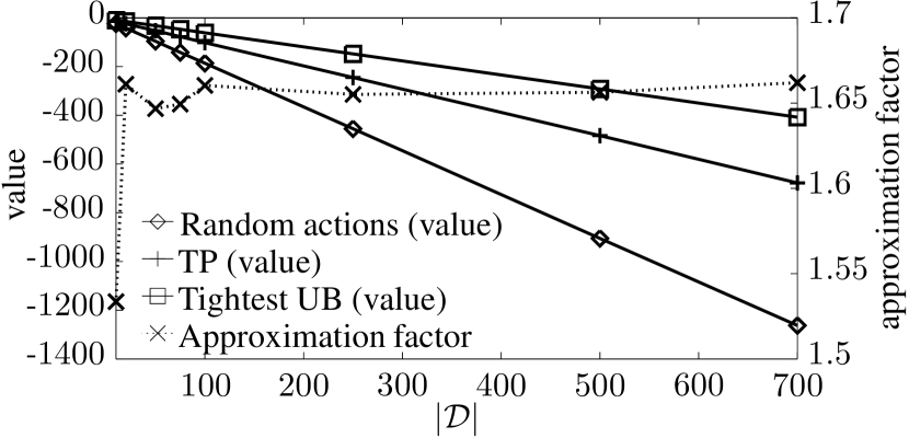
Figure 5: The global IO-Q-Dec-POMDP upper bound on large FFG instances.

We computed upper bounds for large, horizon $h=4$, FFG instances. The computation of the local upper bounds for the largest SPs used (i.e., $|\mathcal{D}^{\prime}|=5$) took 3.31 secs for IO-Q-MMDP and 2696.23s for IO-Q-Dec-POMDP. Fig. 5 shows the results that indicate that the upper bound is relatively tight: the solutions found by TP are not too far from the upper bound. In particular, the EAF lies typically between 1.4 and 1.7, thus providing firm guarantees for solutions of factored Dec-POMDPs with up to 700 agents. Moreover, we see that the EAF stays roughly constant for the larger problem instances indicating that relative guarantees do not degrade as the number of agents increase. Of course, the question of whether the optimal value lies closer to the blue (UB) or orange (TP) line remains open; only further research on improved (heuristic) solution methods and tighter upper bounds can answer that question. However, we have gone from a situation where the only upper bound we had was ‘predict $R_{max}$ for every stage’ (which corresponds to the value 0 and EAF=$\infty$) to a situation where we have a much more informative bound.

Results obtained for a similar approach for Aloha using SPs containing up to $|\mathcal{D}^{\prime}|=6$ agents are shown in Table 1. The numbers clearly illustrate that it is possible to provide very strong guarantees for problems up to $|\mathcal{D}|=250$ agents (beyond which memory forms the bottleneck for TP); the solution for the $|\mathcal{D}|=50$ instance is essentially optimal, indicating also a very tight bound for this problem.

$|\mathcal{D}|$	50	75	100	250
$V^{TP}$	$-71.99$	$-111.07$	$-148.70$	$-382.47$
$\hat{V}^{IO}$	$-72.00$	$-107.06$	$-144.00$	$-360.00$
EAF	$1.00$	$1.04$	$1.03$	$1.06$

Table 1: Empirical approximation factors for Aloha ($h=3$) with varying number of agents.

6.4 Improved Heuristic Influence Search

Aside from analyzing the solution quality of approximate methods, our bounds can also be used in optimal methods. In particular, A*-OIS Witwicki12AAMAS solves TD-POMDPs (a sub-class of factored Dec-POMDPs) by decomposing them into 1-agent SPs, searching through the space of influences, and pruning using optimistic heuristics. However, existing A*-OIS heuristics treat the unspecified-influence stages of the SPs as fully-observable. In contrast, IO-Q-MPOMDP models the partial observability of the SPs.

We now present results that suggest an added computational benefit to treating partial observability in the A*-OIS heuristics. Table 2 illustrates the differences in pruning afforded by four different A*-OIS heuristics: M is the baseline MDP-based heuristic from Witwicki12AAMAS , P is shorthand for IO-Q-MPOMDP, and M’ and P’ are variations that improve tightness with locally-derived probability bounds on the optimistic influences. We report node counts and runtime across several problem instances from the HouseSearch domain Witwicki12AAMAS .

As shown, the POMDP-based heuristics tends to allow for more pruning (fewer expanded nodes) and thereby reduced computation in comparison to their MDP-based counterparts. Contrasting this reduction across two variants of Diamond HouseSearch suggests that the IO-Q-MPOMDP heuristics gain more advantage when observability is more restricted. However, this advantage is sometimes outweighed by the increased computational overhead of a more complex heuristic calculation (such as in Squares HouseSearch $h=4$). The question of predicting in advance when this will be the case is interesting, but difficult (and orthogonal to our contribution).

	$h$=2			$h$=3			$h$=4			$h$=5
HouseSearch : Diamond : $Pr(\text{correct obs.})=0.75$
	#	$s$		#	$s$		#	$s$		#	$s$
M	55	2.36		245	33.86		2072	1179
P	55	2.42		241	34.21		1744	1010
M’	45	2.00		91	9.00		183	64.32		97	991.2
P’	45	2.02		91	10.05		119	39.84		66	607.9
HouseSearch : Diamond : $Pr(\text{correct obs.})=0.5$
	#	$s$		#	$s$		#	$s$		#	$s$
M	47	3.35		225	51.80		1434	1935
P	47	3.32		223	52.75		1416	1905
M’	23	1.96		24	4.69		41	38.42		148	1882
P’	11	0.89		15	3.90		19	25.32		23	256.8
HouseSearch : Squares : $Pr(\text{correct obs.})=0.75$
	#	$s$		#	$s$		#	$s$
M	25	2.41		311	120.5		1323	5846
P	25	2.56		311	121.3		1032	7184
M’	25	2.61		277	109.6		816	3924
P’	25	2.53		240	95.28		752	6760

Table 2: Node count and run time for A*-OIS.

7 Related Work

Here we provide an overview of related approaches.

Scalable Heuristic Methods

In recent years, many scalable approaches without guarantees have been developed for Dec-POMDPs and related models Kumar09AAMAS ; Wu10AAAI ; Yin11IJCAI ; Kumar11IJCAI ; Velagapudi11AAMAS ; Varakantham12AAAI ; Oliehoek13AAMAS ; Wu13IJCAI ; Varakantham14AAAI . The upper bounding mechanism that we propose could be useful for benchmarking many of these methods.

Sub-Problems vs. Source Problems

The use of sub-problems (SPs) is conceptually similar to the use of source problems in transfer planning (TP) Oliehoek13AAMAS . Differences are that, in our partitioning-based upper bounding scheme, SPs are selected such that they do not contain overlapping rewards, while TP allows for overlapping source problems. Moreover TP does not consider optimistic influences but implicitly assumes arbitrary influences. Finally, TP is used as a way to compute a heuristic for the original problem; our approach here simply returns a scalar value (although extensions to use IO heuristics for heuristic search for factored Dec-POMDPs are an interesting direction for future research).

Optimism with Respect to Influences

Being optimistic with respect to external influences has been considered before. For instance, Kumar & Zilberstein Kumar09AAMAS make optimistic assumptions on transitions in an ND-POMDP to derive an MMDP-based policy which is used to sample belief points for memory-bounded dynamic programming. The approach does not use these assumptions to upper bound the global value and the formulation is specific to ND-POMDPs. As described in the experiments, Witwicki, Oliehoek & Kaelbling Witwicki12AAMAS use a local upper bound in order to perform heuristic influence search for TD-POMDPs. IO-Q-MMDP can be seen as a generalization of that heuristic to both factored Dec-POMDPs and multiagent sub-problems, while our other heuristics additionally deal with partial observability.

Quality Guarantees for Large Dec-POMDPs

As mentioned in the introduction, a few approaches to computing upper bound for large-scale MASs and employing them in heuristic search methods have been proposed. In particular, there are some scalable approaches with guarantees for the case of transition and observation independence as encountered in TOI-MDPs and ND-POMDPs Becker03AAMAS ; Becker04AAMAS ; Varakantham07AAMAS ; Marecki08AAMAS ; Dibangoye13AAMAS ; Dibangoye14AAMAS . The approach by Witwicki for TD-POMDPs (Witwicki11PhD, , Sect. 6.6) is a bit more general in that it allows some forms of transition dependence, as long as the interactions are directed (one agent can affect another) and no two agents can affect the same factor in the same stage. In addition, scalability relies on each agent having only a handful of ‘interaction ancestors’.

However, these previous approaches rely on the true value function being factored as the sum of a set $\mathcal{E}$ of local value components:

$$V(\pi)=\sum_{e\in\mathcal{E}}{V}_{e}({\pi}_{e}),$$

where ${\pi}_{e}$ is the local joint policy of the agents that participate in component $e$. (This is also referred to as the ‘value factorization’ framework Kumar11IJCAI ). For this setting, an upper bound is easily constructed as the sum of local upper bounds:

$$\hat{V}(\pi)=\sum_{e\in\mathcal{E}}\hat{{V}_{e}}({\pi}_{e}).$$

While this resembles our IO upper bound (14), the crucial distinction is that for value factorized settings computing $\hat{{V}_{e}}$ does not require any influence-optimism: the reason that value-factorization holds is precisely because there are no influence sources for the components. As such, our influence-optimistic upper bounds can be seen as a strict generalization of the upper bounds that have been employed for settings with factored value functions. Investigating if such methods, such as the method by Dibangoye et al. Dibangoye14AAMAS can be modified to use our IO-UBs is an interesting direction of future work.

Finally, the event-detecting multiagent MDP Kumar09IJCAI provides quality guarantees for a specific class of sensor network problems by using the theory of submodular function maximization. It is the only previous method with quality guarantees that delivers scalability with respect to the number of agents without assuming that the value function of the problem is additively factored into small components.

8 Conclusions

We presented a family of influence-optimistic upper bounds for the value of sub-problems of factored Dec-POMDPs, together with a partition-based decomposition approach that enables the computation of global upper bounds for very large problems. The approach builds upon the framework of influence-based abstraction Oliehoek12AAAI_IBA , but—in contrast to that work—makes optimistic assumptions on the incoming ‘influences’, which makes the sub-problems easier to solve. An empirical evaluation compares the proposed upper bounds and demonstrates that it is possible to achieve guarantees for problems with hundreds of agents, showing that found heuristic solution are in fact close to optimal (empirical approximation factors of $<1.7$ in all cases and sometimes substantially better). This is a significant contribution, given the complexity of computing $\epsilon$-approximate solutions and the fact that tight global upper bounds are of crucial importance to interpret the quality of heuristic solutions.

Intuitively, the proposed approach is expected to work well in settings where the Dec-POMDP is ‘weakly’ coupled. The work by Witwicki & Durfee Witwicki11AAMAS identifies three dimensions that can be used to quantify the notion of weak coupling. Our experiments suggest the existence of a new dimension that can be thought of as influence strength. This dimension captures the impact of non-local behavior on local values and thus directly relates to how well a problem can be approximated using localized components.

In this paper we focused on the finite-horizon case, but the principle of influence optimism underlying the upper-bounding approach can also be applied in infinite-horizon settings. Furthermore, the approach can be modified to compute ‘pessimistic’ influence (i.e., lower) bounds, which could be useful in competitive settings, or for risk-sensitive planning marecki10AAMAS . It is also immediately applicable to problems involving ‘unpredictable’ dynamics Witwicki13ICAPS ; delgado11AIJ . Finally, our upper-bounding method contributes a useful precursor for techniques that automatically search the space of possible upper bounds decompositions, efficient optimal influence-space heuristic search methods (for which we provided preliminary evidence in this paper), and A* methods for a large class of factored Dec-POMDPs. In particular, a promising idea is to employ our factored upper bounds in combination with the heuristic search methods by Dibangoye et al. Dibangoye14AAMAS . While it is not possible to directly use that method since it additionally requires a factored lower bound function, pessimistic-influence bounds could provide those.

A limitation of the current approach is that sub-problems still need to be relatively small, since we rely on optimal optimistic solution of the sub-problems. Developing more scalable ‘optimistic solution methods’ thus is an important direction of future work. Experiments with influence search indicate that using probabilistic bounds on the positive influences has a major impact Witwicki12AAMAS . As such, another important direction of future work is investigating if it is possible to develop tighter upper bounds by making more realistic optimistic assumptions.

Acknowledgments

F.O. is supported by NWO Innovational Research Incentives Scheme Veni #639.021.336.

Appendix A Proofs

Lemma 7. Let ${\pi}_{c}^{t:h-1}$ be a $(h-t)$-steps-to-go policy. Let $\nu\in\mathcal{V}$ and $\nu_{IO}\in\mathcal{V}_{IO}$ be the vectors induced by ${\pi}_{c}^{t:h-1}$ under regular MPOMDP back-projections (for some ${I}_{\rightarrow c}$), and under IO back-projections. Then

$$\forall_{{{x}_{c}^{t}}}\qquad\max_{{D}_{c}^{t+1}}\nu(\langle{{x}_{c}^{t}},{D}_{c}^{t+1}\rangle)\leq\nu_{IO}({{x}_{c}^{t}}).$$

Proof.

The proof is via induction. The base case is for the last stage $t=h-1$, in which case the vectors only consist of the immediate reward:

$$\max_{{D}_{c}^{t+1}}\nu(\langle{{x}_{c}^{t}},{D}_{c}^{t+1}\rangle)=\max_{{D}_{c}^{t+1}}R_{{a}^{t}}({{x}_{c}^{t}})=R_{{a}^{t}}({{x}_{c}^{t}})=\nu_{IO}({{x}_{c}^{t}}),$$

where ${a}^{t}$ is the joint action specified by ${\pi}_{c}^{h-1:h-1}$, thus proving the base case. The induction step follows.

Induction Hypothesis: Suppose that, given that $\nu\in\mathcal{V}$ and $\nu_{IO}\in\mathcal{V}_{IO}$ are vectors for the same policy ${\pi}_{c}^{t+1:h-1}$, for all ${{x}_{c}^{t+1}}$

$$\max_{{D}_{c}^{t+2}}\nu(\langle{{x}_{c}^{t+1}},{D}_{c}^{t+2}\rangle)\leq\nu_{IO}({{x}_{c}^{t+1}})$$ (15)

holds.

To prove: Given that $\nu\in\mathcal{V}$ and $\nu_{IO}\in\mathcal{V}_{IO}$ are vectors for the same policy ${\pi}_{c}^{t:h-1}$, for all ${{x}_{c}^{t}}$

$$\max_{{D}_{c}^{t+1}}\nu(\langle{{x}_{c}^{t}},{D}_{c}^{t+1}\rangle)\leq\nu_{IO}({{x}_{c}^{t}}).$$ (16)

Proof:

We first define the vectors from the l.h.s. Let ${{{a}}^{t}}$ denote the first joint action specified by ${\pi}_{c}^{t:h-1}$. Then we can write

$$\nu(\langle{{x}_{c}^{t}},{D}_{c}^{t+1}\rangle)=r_{a}({{x}_{c}^{t}})+\gamma\sum_{{{o}^{t+1}}}\nu^{\pi|ao}(\langle{{x}_{c}^{t}},{D}_{c}^{t+1}\rangle)$$ (17)

where $\nu^{\pi|ao}$ is the back-projection of the vector $\Gamma({\pi}_{c}^{t:h-1},{{a}_{c}^{t}},{{o}_{c}^{t+1}})$ that corresponds to ${\pi}_{c}^{t+1:h-1}={\pi}_{c}^{t:h-1}\Downarrow_{a,o}$ (the sub-tree of ${\pi}_{c}^{t:h-1}$ given ${{a}_{c}^{t}},{{o}_{c}^{t+1}}$). That is, by filling out the definition of back-projection, we get

$$\nu(\langle{{x}_{c}^{t}},{D}_{c}^{t+1}\rangle)=r_{a}({{x}_{c}^{t}})+\gamma\sum_{{{o}^{t+1}}}\left[\sum_{{{x}_{c}^{t+1}}}\bar{O}({{o}^{t+1}}|{{{a}}^{t}},{{x}_{c}^{t+1}})\bar{T}_{{I}_{\rightarrow c}}({{x}_{c}^{t+1}}|\langle{{x}_{c}^{t}},{D}_{c}^{t+1}\rangle,{{a}_{c}^{t}})[\Gamma({\pi}_{c}^{t:h-1},{{a}_{c}^{t}},{{o}_{c}^{t+1}})](\langle{{x}_{c}^{t+1}},{D}_{c}^{t+2}\rangle)\right],$$

where ${D}_{c}^{t+2}$ is specified as a function of ${{x}_{c}^{t}},{D}_{c}^{t+1},{{{a}}^{t}},{{x}_{c}^{t+1}}$. Clearly, introducing a maximization can not decrease the value, so

$$\nu(\langle{{x}_{c}^{t}},{D}_{c}^{t+1}\rangle) \leq r_{a}({{x}_{c}^{t}})+\gamma\sum_{{{o}^{t+1}}}\sum_{{{x}_{c}^{t+1}}}\bar{O}({{o}^{t+1}}|{{{a}}^{t}},{{x}_{c}^{t+1}})\bar{T}_{{I}_{\rightarrow c}}({{x}_{c}^{t+1}}|\langle{{x}_{c}^{t}},{D}_{c}^{t+1}\rangle,{{a}_{c}^{t}})\max_{{D}_{c}^{t+2}}[\Gamma({\pi}_{c}^{t:h-1},{{a}_{c}^{t}},{{o}_{c}^{t+1}})](\langle{{x}_{c}^{t+1}},{D}_{c}^{t+2}\rangle)$$

{I.H.} $$\leq r_{a}({{x}_{c}^{t}})+\gamma\sum_{{{o}^{t+1}}}\sum_{{{x}_{c}^{t+1}}}\bar{O}({{o}^{t+1}}|{{{a}}^{t}},{{x}_{c}^{t+1}})\bar{T}_{{I}_{\rightarrow c}}({{x}_{c}^{t+1}}|\langle{{x}_{c}^{t}},{D}_{c}^{t+1}\rangle,{{a}_{c}^{t}})[\Gamma_{IO}({\pi}_{c}^{t:h-1},{{a}_{c}^{t}},{{o}_{c}^{t+1}})]({{x}_{c}^{t+1}})$$ (18)

where $\Gamma_{IO}({\pi}_{c}^{t:h-1},{{a}_{c}^{t}},{{o}_{c}^{t+1}})$ is the IO vector that corresponds to ${\pi}_{c}^{t+1:h-1}={\pi}_{c}^{t:h-1}\Downarrow_{a,o}$ .

Now we define the r.h.s. vector:

$$\nu_{IO}({{x}_{c}^{t}})=r_{a}({{x}_{c}^{t}})+\gamma\sum_{{{o}^{t+1}}}\nu_{IO}{}^{\pi|ao}({{x}_{c}^{t}})\\ =r_{a}({{x}_{c}^{t}})+\gamma\sum_{{{o}^{t+1}}}\left[\max_{{u}_{c}^{t+1}}\sum_{{{x}_{c}^{t+1}}}O({{o}_{c}^{t+1}}|{{a}_{c}},{{x}_{c}^{t+1}})\Pr({{xn}_{c}^{t+1}}|{{x}_{c}^{t}},{{a}_{c}},{u}_{c}^{t+1})\Pr({{xl}_{c}^{t+1}}|{{x}_{c}^{t}},{{a}_{c}})[\Gamma_{IO}({\pi}_{c}^{t:h-1},{{a}_{c}^{t}},{{o}_{c}^{t+1}})]({{x}_{c}^{t+1}})\right]$$ (19)

We need to show that

$$\max_{{D}_{c}^{t+1}}\left[r_{a}({{x}_{c}^{t}})+\gamma\sum_{{{o}^{t+1}}}\sum_{{{x}_{c}^{t+1}}}\bar{O}({{o}^{t+1}}|{{{a}}^{t}},{{x}_{c}^{t+1}})\bar{T}_{{I}_{\rightarrow c}}({{x}_{c}^{t+1}}|\langle{{x}_{c}^{t}},{D}_{c}^{t+1}\rangle,{{a}_{c}^{t}})[\Gamma_{IO}({\pi}_{c}^{t:h-1},{{a}_{c}^{t}},{{o}_{c}^{t+1}})]({{x}_{c}^{t+1}})\right]\\ \leq r_{a}({{x}_{c}^{t}})+\gamma\sum_{{{o}^{t+1}}}\max_{{u}_{c}^{t+1}}\sum_{{{x}_{c}^{t+1}}}O({{o}_{c}^{t+1}}|{{a}_{c}},{{x}_{c}^{t+1}})\Pr({{xn}_{c}^{t+1}}|{{x}_{c}^{t}},{{a}_{c}},{u}_{c}^{t+1})\Pr({{xl}_{c}^{t+1}}|{{x}_{c}^{t}},{{a}_{c}})[\Gamma_{IO}({\pi}_{c}^{t:h-1},{{a}_{c}^{t}},{{o}_{c}^{t+1}})]({{x}_{c}^{t+1}})$$

which holds if and only if

$$\max_{{D}_{c}^{t+1}}\sum_{{{o}^{t+1}}}\sum_{{{x}_{c}^{t+1}}}\bar{O}({{o}^{t+1}}|{{{a}}^{t}},{{x}_{c}^{t+1}})\bar{T}_{{I}_{\rightarrow c}}({{x}_{c}^{t+1}}|\langle{{x}_{c}^{t}},{D}_{c}^{t+1}\rangle,{{a}_{c}^{t}})[\Gamma_{IO}({\pi}_{c}^{t:h-1},{{a}_{c}^{t}},{{o}_{c}^{t+1}})]({{x}_{c}^{t+1}})\\ \leq\sum_{{{o}^{t+1}}}\max_{{u}_{c}^{t+1}}\sum_{{{x}_{c}^{t+1}}}O({{o}_{c}^{t+1}}|{{a}_{c}},{{x}_{c}^{t+1}})\Pr({{xn}_{c}^{t+1}}|{{x}_{c}^{t}},{{a}_{c}},{u}_{c}^{t+1})\Pr({{xl}_{c}^{t+1}}|{{x}_{c}^{t}},{{a}_{c}})[\Gamma_{IO}({\pi}_{c}^{t:h-1},{{a}_{c}^{t}},{{o}_{c}^{t+1}})]({{x}_{c}^{t+1}}).$$ (20)

To show this is the case, we start with the l.h.s.:

$$\max_{{D}_{c}^{t+1}}\sum_{{{o}^{t+1}}}\sum_{{{x}_{c}^{t+1}}}\bar{O}({{o}^{t+1}}|{{{a}}^{t}},{{x}_{c}^{t+1}})\bar{T}_{{I}_{\rightarrow c}}({{x}_{c}^{t+1}}|\langle{{x}_{c}^{t}},{D}_{c}^{t+1}\rangle,{{a}_{c}^{t}})[\Gamma_{IO}({\pi}_{c}^{t:h-1},{{a}_{c}^{t}},{{o}_{c}^{t+1}})]({{x}_{c}^{t+1}})$$

$$= \max_{{D}_{c}^{t+1}}\sum_{{{o}^{t+1}}}\sum_{{{x}_{c}^{t+1}}}\bar{O}({{o}^{t+1}}|{{{a}}^{t}},{{x}_{c}^{t+1}})\left[\sum_{{u}_{c}^{t+1}}\Pr({{xn}_{i}^{t+1}}|{{x}_{c}^{t}},{{a}_{c}^{t}},{u}_{c}^{t+1})I({u}_{c}^{t+1}|{D}_{c}^{t+1})\right]\Pr({{xl}_{c}^{t+1}}|{{x}_{c}^{t}},{{a}_{c}^{t}})[\Gamma_{IO}({\pi}_{c}^{t:h-1},{{a}_{c}^{t}},{{o}_{c}^{t+1}})]({{x}_{c}^{t+1}})$$

$$= \max_{{D}_{c}^{t+1}}\sum_{{{o}^{t+1}}}\sum_{{u}_{c}^{t+1}}I({u}_{c}^{t+1}|{D}_{c}^{t+1})\sum_{{{x}_{c}^{t+1}}}\bar{O}({{o}^{t+1}}|{{{a}}^{t}},{{x}_{c}^{t+1}})\Pr({{xn}_{i}^{t+1}}|{{x}_{c}^{t}},{{a}_{c}^{t}},{u}_{c}^{t+1})\Pr({{xl}_{c}^{t+1}}|{{x}_{c}^{t}},{{a}_{c}^{t}})[\Gamma_{IO}({\pi}_{c}^{t:h-1},{{a}_{c}^{t}},{{o}_{c}^{t+1}})]({{x}_{c}^{t+1}})$$

$$= \max_{{D}_{c}^{t+1}}\sum_{{{o}^{t+1}}}\sum_{{u}_{c}^{t+1}}I({u}_{c}^{t+1}|{D}_{c}^{t+1})\left[\sum_{{{x}_{c}^{t+1}}}\bar{O}({{o}^{t+1}}|{{{a}}^{t}},{{x}_{c}^{t+1}})\Pr({{xn}_{i}^{t+1}}|{{x}_{c}^{t}},{{a}_{c}^{t}},{u}_{c}^{t+1})\Pr({{xl}_{c}^{t+1}}|{{x}_{c}^{t}},{{a}_{c}^{t}})[\Gamma_{IO}({\pi}_{c}^{t:h-1},{{a}_{c}^{t}},{{o}_{c}^{t+1}})]({{x}_{c}^{t+1}})\right]$$

$$\leq$$ {max. of a function is greater than its expectation:}

$$\max_{{D}_{c}^{t+1}}\sum_{{{o}^{t+1}}}\max_{{u}_{c}^{t+1}}\left[\sum_{{{x}_{c}^{t+1}}}\bar{O}({{o}^{t+1}}|{{{a}}^{t}},{{x}_{c}^{t+1}})\Pr({{xn}_{i}^{t+1}}|{{x}_{c}^{t}},{{a}_{c}^{t}},{u}_{c}^{t+1})\Pr({{xl}_{c}^{t+1}}|{{x}_{c}^{t}},{{a}_{c}^{t}})[\Gamma_{IO}({\pi}_{c}^{t:h-1},{{a}_{c}^{t}},{{o}_{c}^{t+1}})]({{x}_{c}^{t+1}})\right]$$

$$= {D}_{c}^{t+1}$$ {no dependence on anymore:}

$$\sum_{{{o}^{t+1}}}\max_{{u}_{c}^{t+1}}\sum_{{{x}_{c}^{t+1}}}\bar{O}({{o}^{t+1}}|{{{a}}^{t}},{{x}_{c}^{t+1}})\Pr({{xn}_{i}^{t+1}}|{{x}_{c}^{t}},{{a}_{c}^{t}},{u}_{c}^{t+1})\Pr({{xl}_{c}^{t+1}}|{{x}_{c}^{t}},{{a}_{c}^{t}})[\Gamma_{IO}({\pi}_{c}^{t:h-1},{{a}_{c}^{t}},{{o}_{c}^{t+1}})]({{x}_{c}^{t+1}})$$

which is the r.h.s. of (20), the inequality the we needed to demonstrate, thereby finishing the proof.∎

References

- [1] C. Amato and F. A. Oliehoek. Bayesian reinforcement learning for multiagent systems with state uncertainty. In AAMAS Workshop on Multi-Agent Sequential Decision Making in Uncertain Domains (MSDM), pages 76–83, 2013.
- [2] R. Becker, S. Zilberstein, and V. Lesser. Decentralized Markov decision processes with event-driven interactions. In Proc. of the International Conference on Autonomous Agents and Multiagent Systems, pages 302–309, 2004.
- [3] R. Becker, S. Zilberstein, V. Lesser, and C. V. Goldman. Transition-independent decentralized Markov decision processes. In Proc. of the International Conference on Autonomous Agents and Multiagent Systems, pages 41–48, 2003.
- [4] C. Boutilier, T. Dean, and S. Hanks. Decision-theoretic planning: Structural assumptions and computational leverage. Journal of Artificial Intelligence Research, 11:1–94, 1999.
- [5] C. Boutilier and D. Poole. Computing optimal policies for partially observable decision processes using compact representations. In Proc. of the National Conference on Artificial Intelligence, pages 1168–1175, 1996.
- [6] A. Cassandra, M. L. Littman, and N. L. Zhang. Incremental pruning: A simple, fast, exact method for partially observable Markov decision processes. In Proc. of Uncertainty in Artificial Intelligence, pages 54–61, 1997.
- [7] K. V. Delgado, S. Sanner, and L. N. De Barros. Efficient solutions to factored MDPs with imprecise transition probabilities. Artificial Intelligence, 175(9):1498–1527, 2011.
- [8] J. S. Dibangoye, C. Amato, O. Buffet, and F. Charpillet. Optimally solving Dec-POMDPs as continuous-state MDPs. In Proc. of the International Joint Conference on Artificial Intelligence, 2013.
- [9] J. S. Dibangoye, C. Amato, O. Buffet, and F. Charpillet. Exploiting separability in multiagent planning with continuous-state MDPs. In Proc. of the International Conference on Autonomous Agents and Multiagent Systems, pages 1281–1288, 2014.
- [10] J. S. Dibangoye, C. Amato, A. Doniec, and F. Charpillet. Producing efficient error-bounded solutions for transition independent decentralized MDPs. In Proc. of the International Conference on Autonomous Agents and Multiagent Systems, pages 539–546, 2013.
- [11] R. Emery-Montemerlo, G. Gordon, J. Schneider, and S. Thrun. Approximate solutions for partially observable stochastic games with common payoffs. In Proc. of the International Conference on Autonomous Agents and Multiagent Systems, pages 136–143, 2004.
- [12] E. A. Hansen, D. S. Bernstein, and S. Zilberstein. Dynamic programming for partially observable stochastic games. In Proc. of the National Conference on Artificial Intelligence, pages 709–715, 2004.
- [13] L. P. Kaelbling, M. L. Littman, and A. R. Cassandra. Planning and acting in partially observable stochastic domains. Artificial Intelligence, 101(1-2):99–134, 1998.
- [14] A. Kumar and S. Zilberstein. Constraint-based dynamic programming for decentralized POMDPs with structured interactions. In Proc. of the International Conference on Autonomous Agents and Multiagent Systems, pages 561–568, 2009.
- [15] A. Kumar and S. Zilberstein. Event-detecting multi-agent MDPs: Complexity and constant-factor approximations. In Proc. of the International Joint Conference on Artificial Intelligence, pages 201–207, 2009.
- [16] A. Kumar, S. Zilberstein, and M. Toussaint. Scalable multiagent planning using probabilistic inference. In Proc. of the International Joint Conference on Artificial Intelligence, pages 2140–2146, 2011.
- [17] L. C. MacDermed and C. Isbell. Point based value iteration with optimal belief compression for Dec-POMDPs. In Advances in Neural Information Processing Systems 26, pages 100–108. 2013.
- [18] A. Mahajan and M. Mannan. Decentralized stochastic control. Annals of Operations Research, 2014.
- [19] J. Marecki, T. Gupta, P. Varakantham, M. Tambe, and M. Yokoo. Not all agents are equal: scaling up distributed POMDPs for agent networks. In Proc. of the International Conference on Autonomous Agents and Multiagent Systems, pages 485–492, 2008.
- [20] J. Marecki and P. Varakantham. Risk-sensitive planning in partially observable environments. In Proc. of the International Conference on Autonomous Agents and Multiagent Systems, pages 1357–1368, 2010.
- [21] J. V. Messias, M. T. J. Spaan, and P. U. Lima. Efficient offline communication policies for factored multiagent POMDPs. In NIPS 24, pages 1917–1925. 2011.
- [22] R. Nair, P. Varakantham, M. Tambe, and M. Yokoo. Networked distributed POMDPs: A synthesis of distributed constraint optimization and POMDPs. In Proc. of the National Conference on Artificial Intelligence, pages 133–139, 2005.
- [23] F. A. Oliehoek and C. Amato. Dec-POMDPs as non-observable MDPs. Technical report, University of Amsterdam, 2014.
- [24] F. A. Oliehoek, M. T. J. Spaan, C. Amato, and S. Whiteson. Incremental clustering and expansion for faster optimal planning in decentralized POMDPs. Journal of AI Research, 46:449–509, 2013.
- [25] F. A. Oliehoek, M. T. J. Spaan, and N. Vlassis. Optimal and approximate Q-value functions for decentralized POMDPs. Journal of AI Research, 32:289–353, 2008.
- [26] F. A. Oliehoek, M. T. J. Spaan, S. Whiteson, and N. Vlassis. Exploiting locality of interaction in factored Dec-POMDPs. In Proc. of the International Conference on Autonomous Agents and Multiagent Systems, pages 517–524, 2008.
- [27] F. A. Oliehoek, S. Whiteson, and M. T. J. Spaan. Approximate solutions for factored Dec-POMDPs with many agents. In Proc. of the International Conference on Autonomous Agents and Multiagent Systems, pages 563–570, 2013.
- [28] F. A. Oliehoek, S. Witwicki, and L. P. Kaelbling. Influence-based abstraction for multiagent systems. In Proc. of the AAAI Conference on Artificial Intelligence, pages 1422–1428, 2012.
- [29] J. M. Ooi and G. W. Wornell. Decentralized control of a multiple access broadcast channel: Performance bounds. In Proc. of the 35th Conference on Decision and Control, pages 293–298, 1996.
- [30] J. Pajarinen and J. Peltonen. Efficient planning for factored infinite-horizon DEC-POMDPs. In Proc. of the International Joint Conference on Artificial Intelligence, pages 325–331, 2011.
- [31] Z. Rabinovich, C. V. Goldman, and J. S. Rosenschein. The complexity of multiagent systems: the price of silence. In Proc. of the International Conference on Autonomous Agents and Multiagent Systems, pages 1102–1103, 2003.
- [32] M. Roth, R. Simmons, and M. Veloso. Reasoning about joint beliefs for execution-time communication decisions. In Proc. of the International Conference on Autonomous Agents and Multiagent Systems, pages 786–793, 2005.
- [33] G. Shani, J. Pineau, and R. Kaplow. A survey of point-based POMDP solvers. Autonomous Agents and Multi-Agent Systems, 27(1):1–51, 2013.
- [34] M. T. J. Spaan. Partially observable Markov decision processes. In Reinforcement Learning: State of the Art, pages 387–414. Springer Verlag, 2012.
- [35] D. Szer, F. Charpillet, and S. Zilberstein. MAA*: A heuristic search algorithm for solving decentralized POMDPs. In Proc. of Uncertainty in Artificial Intelligence, pages 576–583, 2005.
- [36] P. Varakantham, Y. Adulyasak, and P. Jaillet. Decentralized stochastic planning with anonymity in interactions. In Proc. of the AAAI Conference on Artificial Intelligence, pages 2505–2512, 2014.
- [37] P. Varakantham, S. Cheng, G. J. Gordon, and A. Ahmed. Decision support for agent populations in uncertain and congested environments. In Proc. of the AAAI Conference on Artificial Intelligence, 2012.
- [38] P. Varakantham, J. Marecki, Y. Yabu, M. Tambe, and M. Yokoo. Letting loose a SPIDER on a network of POMDPs: Generating quality guaranteed policies. In Proc. of the International Conference on Autonomous Agents and Multiagent Systems, 2007.
- [39] V. V. Vazirani. Approximation Algorithms. Springer-Verlag, 2001.
- [40] P. Velagapudi, P. Varakantham, P. Scerri, and K. Sycara. Distributed model shaping for scaling to decentralized POMDPs with hundreds of agents. In Proc. of the International Conference on Autonomous Agents and Multiagent Systems, 2011.
- [41] S. Witwicki, F. A. Oliehoek, and L. P. Kaelbling. Heuristic search of multiagent influence space. In Proc. of the International Conference on Autonomous Agents and Multiagent Systems, pages 973–981, 2012.
- [42] S. J. Witwicki. Abstracting Influences for Efficient Multiagent Coordination Under Uncertainty. PhD thesis, University of Michigan, 2011.
- [43] S. J. Witwicki and E. H. Durfee. Influence-based policy abstraction for weakly-coupled Dec-POMDPs. In Proc. of the International Conference on Automated Planning and Scheduling, pages 185–192, 2010.
- [44] S. J. Witwicki and E. H. Durfee. Towards a unifying characterization for quantifying weak coupling in Dec-POMDPs. In Proc. of the International Conference on Autonomous Agents and Multiagent Systems, pages 29–36, 2011.
- [45] S. J. Witwicki, F. S. Melo, J. C. Fernández, and M. T. J. Spaan. A flexible approach to modeling unpredictable events in MDPs. In Proc. of the International Conference on Automated Planning and Scheduling, pages 260–268, 2013.
- [46] F. Wu, S. Zilberstein, and X. Chen. Trial-based dynamic programming for multi-agent planning. In Proc. of the AAAI Conference on Artificial Intelligence, pages 908–914, 2010.
- [47] F. Wu, S. Zilberstein, and N. R. Jennings. Monte-Carlo expectation maximization for decentralized POMDPs. In Proc. of the International Joint Conference on Artificial Intelligence, pages 397–403, 2013.
- [48] Z. Yin and M. Tambe. Continuous time planning for multiagent teams with temporal constraints. In Proc. of the International Joint Conference on Artificial Intelligence, 2011.