Pathwise Sensitivity Analysis in Transient Regimes

Abstract

The instantaneous relative entropy (IRE) and the corresponding instantaneous Fisher information matrix (IFIM) for transient stochastic processes are presented in this paper. These novel tools for sensitivity analysis of stochastic models serve as an extension of the well known relative entropy rate (RER) and the corresponding Fisher information matrix (FIM) that apply to stationary processes. Three cases are studied here, discrete-time Markov chains, continuous-time Markov chains and stochastic differential equations. A biological reaction network is presented as a demonstration numerical example.

1 Introduction

Sensitivity analysis, for a general mathematical model, is defined to be the quantification of system response to parameter perturbations. Questions on the robustness, (structural) identifiability, experimental design, uncertainty quantification, estimation and control can be addressed through sensitivity analysis [1]. Moreover, it is a necessary analysis tool for the study of kinetic models such as chemical and biochemical reaction networks [1, 2]. The mathematical models considered in this paper are models that describe phenomena exhibiting stochasticity: stochastic differential equations (SDE), discrete-time and continuous-time Markov chains (DTMC and CTMC). Some of the mathematical tools for the sensitivity analysis of such systems include log-likelihood methods and Girsanov transformations [3, 4, 5], polynomial chaos [6], finite difference methods [7, 8] and pathwise sensitivity methods [9]. Closely related to the log-likelihood methods are various linear-response-based approaches, for instance in the context of chemical kinetics [10], as well as in recent mathematical work for linear response in non-equilibrium systems [11, 12].

In [13], the authors propose a new methodology for the pathwise sensitivity analysis of complex stochastic stationary dynamics based on the Relative Entropy (RE) between path distributions and Relative Entropy Rate (RER). This two quantities provide a measure of the sensitivity of the entire time-series distribution. The space of all such time-series is referred in probability theory as the “path space”. RER measures the loss of information per unit time in path space after an arbitrary perturbation of parameter combinations. Moreover, RER and the corresponding Fisher Information Matrix (FIM) become computationally feasible in certain cases as they admit explicit formulas. In fact, it is been showed in [13] that the proposed pathwise sensitivity analysis has the following properties: (a) it is rigorously valid for the sensitivity of long-time, stationary dynamics, (b) it is a gradient-free sensitivity analysis method suitable for high-dimensional parameter spaces, (c) the computation of RER and FIM does not require the explicit knowledge of the equilibrium probability distribution, relying only on information for local dynamics, i.e. it is suitable for non-equilibrium systems.

In this paper we extend the RE and FIM tools, developed in [13] for stationary processes, to transient and non-stationary processes. The extension is based on the notion of instantaneous RE (IRE) and instantaneous FIM (IFIM), see for example equations (10) and (12) in text. These sensitivity tools provide an instantaneous measure for the sensitivity of a system arising from information theoretic tools. Moreover, both IRE and IFIM, which are independent of observable functions, can be used as upper bounds for observable depended sensitivities, see for example the discussion in Conclusions and [14, 15].

The rest of the paper is organized as follows: In Section 2 a review of the RE and the FIM is given. In Sections 3,4 and 5 the new quantities IRE and IFIM are presented for discrete-time Markov chains, continuous-time Markov chains and stochastic differential equations, respectively. In Section 6, a numerical example for a biological reaction network is utilized and IRE and IFIM are computed in the course of a stochastic simulation and various observations are discussed. Finally, in Section 7, concluding remarks and connections with existing works are discussed.

2 Time-dependent sensitivity analysis

2.1 Decomposition of the pathwise relative entropy

The relative entropy (or Kullback-Leibler divergence) of a probability measure $P$ with respect to (w.r.t.) another probability measure $\bar{P}$ is defined as [16, 17]

$$\mathcal{R}\left({P}{\,|\,}{\bar{P}}\right):=\left\{\begin{array}[]{ll}\int\log{\frac{dP}{d\bar{P}}}dP\ ,&\ \ P\ll\bar{P}\\ \infty\ ,&\ \ \text{otherwise}\end{array}\right.$$ (1)

where $\frac{dP}{d\bar{P}}$ is a function known as the Radon-Nikodym derivative which is well-defined when $P$ is absolutely continuous w.r.t. $\bar{P}$ (denoted as $P\ll\bar{P}$) while the integration is performed w.r.t. the probability measure $P$. Relative entropy has been utilized in a diverge range of scientific fields from statistical mechanics [18] to telecommunications [17] and finance [19] and possesses the following fundamental properties:

• $\mathcal{R}\left({P}{\,|\,}{\bar{P}}\right)\geq 0$,

• $\mathcal{R}\left({P}{\,|\,}{\bar{P}}\right)=0$ if and only if $P=\bar{P}\;\;P$-almost everywhere, and,

• $\mathcal{R}\left({P}{\,|\,}{\bar{P}}\right)<\infty$ if and only if $P$ and $\bar{P}$ are absolutely continuous w.r.t. each other.

These properties allow us to view relative entropy as a “distance” (more precisely a divergence) between two probability measures capturing the relative importance of uncertainties [20]. From an information theory perspective, relative entropy measures the loss/change of information when $\bar{P}$ is considered instead of $P$ [17].

Let a stochastic process –either discrete-time or continuous-time– be denoted by $X_{t}$ and let the path space $\mathcal{X}$ be the set of all trajectories $\{X_{t}\}_{t=0}^{T}$. We denote by $Q_{0:T}$ the path space distribution, i.e., the probability to see a particular element of path space, $\mathcal{X}$. Denote by $\bar{Q}_{0:T}$ the path space distribution of another process, $\bar{X}_{t}$. The pathwise relative entropy of the distribution $Q_{0:T}$ w.r.t. the distribution $\bar{Q}_{0:T}$ assuming that they are absolutely continuous w.r.t. each other is written using (1) as

$$\mathcal{R}\left({Q_{0:T}}{\,|\,}{\bar{Q}_{0:T}}\right)=\int\log\frac{dQ_{0:T}}{d\bar{Q}_{0:T}}dQ_{0:T}\ .$$ (2)

A key property of pathwise relative entropy is that it is an increasing function of time which is the analog of the second thermodynamic law in statistical physics [17]. To this end, for various important Markov processes, it can be shown, exploiting the Markov property, that the pathwise relative entropy can be written as an averaged quantity as

$$\mathcal{R}\left({Q_{0:T}}{\,|\,}{\bar{Q}_{0:T}}\right)=\left\{\begin{array}[]{ll}\mathcal{R}\left({\nu}{\,|\,}{\bar{\nu}}\right)+\sum_{i=1}^{T}\mathcal{H}\left({Q_{i}}{\,|\,}{\bar{Q}_{i}}\right)\ ,&\text{\ \ if time is discrete}\\ \mathcal{R}\left({\nu}{\,|\,}{\bar{\nu}}\right)+\int_{0}^{T}\mathcal{H}\left({Q_{t}}{\,|\,}{\bar{Q}_{t}}\right)dt\ ,&\text{\ \ if time is continuous}\ ,\end{array}\right.$$ (3)

where $\mathcal{R}\left({\nu}{\,|\,}{\bar{\nu}}\right)$ is the relative entropy of the initial distribution $\nu$ w.r.t. the perturbed initial distribution $\bar{\nu}$, while $\mathcal{H}\left({Q_{\cdot}}{\,|\,}{\bar{Q}_{\cdot}}\right)$ denotes the instantaneous relative entropy (for explicit formulas we refer to equation (10), (16) and (24)). We named the quantity $\mathcal{H}\left({Q_{\cdot}}{\,|\,}{\bar{Q}_{\cdot}}\right)$ instantaneous relative entropy because it is also non-negative but more importantly is the time-derivative of the pathwise relative entropy and inherits the properties of the relative entropy. Notice that the notation for instantaneous relative entropy is somewhat confusing but it will become clear when specific examples will be presented in the following sections.

Moreover the relative entropy rate is defined for a broad class of stochastic processes including Markov and semi-Markov processes as [21] as the limit

$$\mathcal{H}\left({Q}{\,|\,}{\bar{Q}}\right)=\lim_{T\rightarrow\infty}\frac{1}{T}\mathcal{R}\left({Q_{0:T}}{\,|\,}{\bar{Q}_{0:T}}\right)\ .$$ (4)

Relative entropy rate is closely related to the instantaneous relative entropy in two fundamental ways, Firstly it is the limit of instantaneous relative entropy as time goes to infinity, whenever this limit is defined and second it holds at the stationary regime that

$$\mathcal{H}\left({Q_{i}}{\,|\,}{\bar{Q}_{i}}\right)=\mathcal{H}\left({Q}{\,|\,}{\bar{Q}}\right)$$ (5)

for the discrete-time case with $i=1,...,T$ and similarly for the continuous-time case.

2.2 Sensitivity analysis and Fisher information matrix

In [13], authors proposed the relative entropy between path distributions to perform sensitivity analysis arguing that pathwise relative entropy takes into account not only the equilibrium properties but also the complex dynamics of a stochastic process. Specifically, denote by $Q_{0:T}^{\theta}$ the path space distribution of the process $X_{t}$, parametrized by the parameter vector $\theta\in\mathbb{R}^{K}$. Consider also a perturbation vector, $\epsilon\in\mathbb{R}^{K}$, and denote by $Q_{0:T}^{\theta+\epsilon}$ the path space distribution of the perturbed process $\bar{X}_{t}$. The pathwise relative entropy of the distribution $Q_{0:T}^{\theta}$ w.r.t. the distribution $Q_{0:T}^{\theta+\epsilon}$ assuming that they are absolutely continuous w.r.t. each other is written from (2) as

$$\mathcal{R}\left({Q_{0:T}^{\theta}}{\,|\,}{Q_{0:T}^{\theta+\epsilon}}\right)=\int\log\frac{dQ_{0:T}^{\theta}}{dQ_{0:T}^{\theta+\epsilon}}dQ_{0:T}^{\theta}\ .$$ (6)

An attractive approach to sensitivity analysis that is rigorously based on relative entropy calculations is the Fisher Information Matrix (FIM). Indeed, assuming smoothness in the parameter vector, it is straightforward to obtain the following expansion for (6) [17, 22],

$$\mathcal{R}\left({{Q_{0:T}^{\theta}}}{\,|\,}{{Q_{0:T}^{\theta+\epsilon}}}\right)=\frac{1}{2}\epsilon^{T}{\mathcal{I}}\big{(}Q_{0:T}^{\theta}\big{)}\epsilon+O(|\epsilon|^{3})\,,$$ (7)

where the $K\times K$ pathwise FIM ${\mathcal{I}}\big{(}Q_{0:T}^{\theta}\big{)}$ is defined as the Hessian of the pathwise relative entropy. As (7) readily suggests, relative entropy is locally a quadratic function of the parameter vector $\theta$. Indeed, the pathwise RE for any perturbation can be recovered up to third-order utilizing only the pathwise FIM. Moreover, similar expansions hold for the instantaneous relative entropy and the relative entropy rate. The decomposition of the pathwise FIM reads

$${\mathcal{I}}\big{(}Q_{0:T}^{\theta}\big{)}=\left\{\begin{array}[]{ll}{\mathcal{I}}\big{(}\nu^{\theta}\big{)}+\sum_{i=1}^{T}{\mathcal{I}}_{\mathcal{H}}\big{(}Q_{i}^{\theta}\big{)}\ ,&\text{\ \ if time is discrete}\\ {\mathcal{I}}\big{(}\nu^{\theta}\big{)}+\int_{0}^{T}{\mathcal{I}}_{\mathcal{H}}\big{(}Q_{t}^{\theta}\big{)}dt\ ,&\text{\ \ if time is continuous}\end{array}\right.$$ (8)

where ${\mathcal{I}}\big{(}\nu^{\theta}\big{)}$ is the FIM of the initial distribution $\nu^{\theta}$ while ${\mathcal{I}}_{\mathcal{H}}\big{(}Q_{\cdot}^{\theta}\big{)}$ denotes the instantaneous FIM. In the following sections concrete examples of stochastic Markov processes are presented whose pathwise relative entropy and the associated pathwise FIM is provided.

3 Discrete-time Markov chains

This section presents explicit formulas of the various relative entropy quantities defined in the previous section as well as the associated FIMs for the case of discrete-time Markov chains. The analysis of the DTMC case serves (a) as a more intuitive and manageable example of stochastic processes and (b) as a intermediate step to handle the continuous-time Markov chain case.

Next, let $\{x_{i}\}_{i\in\mathbb{Z}^{+}}$ be a discrete-time time-homogeneous Markov chain with separable state space $E$. The transition probability kernel of the Markov chain denoted by $P^{\theta}(x,dx^{\prime})$ depends on the parameter vector $\theta\in\mathbb{R}^{K}$. Assume that the transition kernel is absolutely continuous with respect to the Lebesgue measure and the transition probability density function $p^{\theta}(x,x^{\prime})$ is always positive for all $x,x^{\prime}\in E$ and for all $\theta\in\mathbb{R}^{K}$. Exploiting the Markov property, the path space probability density $Q_{0:T}^{\theta}$ for the path $\{x_{i}\}_{i=0}^{T}$ at the time horizon $0,1,\ldots,T$ starting from the initial distribution $\nu^{\theta}(x)dx$ is given by

$$Q_{0:T}^{\theta}\big{(}x_{0},\ldots,x_{T}\big{)}=\nu^{\theta}(x_{0})p^{\theta}(x_{0},x_{1})\ldots p^{\theta}(x_{T-1},x_{T})\,.$$

We consider a perturbation vector $\epsilon\in\mathbb{R}^{K}$ and the Markov chain $\{\bar{x}_{i}\}_{i\in\mathbb{Z}^{+}}$ with transition probability density function, $p^{\theta+\epsilon}(x,x^{\prime})$, initial density, $\nu^{\theta+\epsilon}(x)$, as well as path distribution $Q_{0:T}^{\theta+\epsilon}$. The product representation of the path distributions results in an additive representation of the relative entropy of the path distribution $Q_{0:T}^{\theta}$ w.r.t. the perturbed path distribution $Q_{0:T}^{\theta+\epsilon}$. Let $\nu_{i}^{\theta}(x)$ denote the probability density function of the Markov chain at time instant $i$ given that the initial distribution is $\nu^{\theta}$, whose formula is provided by the Chapman-Kolmogorov equation,

$$\nu_{i}^{\theta}(x)=\int_{E}\cdots\int_{E}\nu^{\theta}(x_{0})p^{\theta}(x_{0},x_{1})\ldots p^{\theta}(x_{i-1},x)dx_{0}\ldots dx_{i-1}\ .$$

The following theorem presents the decomposition of the pathwise relative entropy.

Theorem 3.1.

(a) The pathwise relative entropy for the above-defined discrete-time Markov chain is decomposed as

$$\mathcal{R}\left({Q_{0:T}^{\theta}}{\,|\,}{Q_{0:T}^{\theta+\epsilon}}\right)=\mathcal{R}\left({\nu^{\theta}}{\,|\,}{\nu^{\theta+\epsilon}}\right)+\sum_{i=1}^{T}\mathcal{H}\left({Q_{i}^{\theta}}{\,|\,}{Q_{i}^{\theta+\epsilon}}\right)\ ,$$ (9)

where the instantaneous relative entropy equals to

$$\mathcal{H}\left({Q_{i}^{\theta}}{\,|\,}{Q_{i}^{\theta+\epsilon}}\right)=\mathbb{E}_{\nu_{i-1}^{\theta}}\Big{[}\int_{E}p^{\theta}(x,x^{\prime})\log\frac{p^{\theta}(x,x^{\prime})}{p^{\theta+\epsilon}(x,x^{\prime})}dx^{\prime}\Big{]}$$ (10)

(b) Under smoothness assumption on the transition probability function for the parameter $\theta$, the pathwise FIM is also decomposed as

$${\mathcal{I}}\big{(}Q_{0:T}^{\theta}\big{)}={\mathcal{I}}\big{(}\nu^{\theta}\big{)}+\sum_{i=1}^{T}{\mathcal{I}}_{\mathcal{H}}\big{(}Q_{i}^{\theta}\big{)}\ ,$$ (11)

where the instantaneous pathwise FIM is given by

$${\mathcal{I}}_{\mathcal{H}}\big{(}Q_{i}^{\theta}\big{)}=\mathbb{E}_{\nu_{i-1}^{\theta}}[\int_{E}p^{\theta}(x,x^{\prime})\nabla_{\theta}\log p^{\theta}(x,x^{\prime})\nabla_{\theta}\log p^{\theta}(x,x^{\prime})^{T}dx^{\prime}]\$$ (12)

Proof.

(a) The proof of this part of the theorem can be found in [17, Ch. 2] under the title “Chain rule for relative entropy” but for the shake of completeness we present it here. The Radon-Nikodym derivative of the unperturbed path distribution w.r.t. the perturbed path distribution takes the form

$$\frac{dQ_{0:T}^{\theta}}{dQ_{0:T}^{\theta+\epsilon}}\big{(}\{x_{i}\}_{i=0}^{T}\big{)}=\frac{\nu^{\theta}(x_{0})\prod_{i=0}^{T-1}p^{\theta}(x_{i},x_{i+1})}{\nu^{\theta+\epsilon}(x_{0})\prod_{i=0}^{T-1}p^{\theta+\epsilon}(x_{i},x_{i+1})}\,,$$

which is well-defined since the transition probabilities are always positive. Then,

$$\mathcal{R}\left({Q_{0:T}^{\theta}}{\,|\,}{Q_{0:T}^{\theta+\epsilon}}\right)$$

$$=\int_{E}\cdots\int_{E}\nu^{\theta}(x_{0})\prod_{j=1}^{T}p^{\theta}(x_{j-1},x_{j})\log\frac{\nu^{\theta}(x_{0})\prod_{i=1}^{T}p^{\theta}(x_{i-1},x_{i})}{\nu^{\theta+\epsilon}(x_{0})\prod_{i=1}^{T}p^{\theta+\epsilon}(x_{i-1},x_{i})}dx_{0}\ldots dx_{T}$$

$$=\int_{E}\cdots\int_{E}\nu^{\theta}(x_{0})\prod_{j=1}^{T}p^{\theta}(x_{j-1},x_{j})\log\frac{\nu^{\theta}(x_{0})}{\nu^{\theta+\epsilon}(x_{0})}dx_{0}\ldots dx_{T}$$

$$\quad+\sum_{i=1}^{T}\int_{E}\cdots\int_{E}\nu^{\theta}(x_{0})\prod_{j=1}^{T}p^{\theta}(x_{j-1},x_{j})\log\frac{p^{\theta}(x_{i-1},X_{i})}{p^{\theta+\epsilon}(x_{i-1},x_{i})}dx_{0}\ldots dx_{T}$$

$$=\mathcal{R}\left({\nu^{\theta}}{\,|\,}{\nu^{\theta+\epsilon}}\right)+\sum_{i=1}^{T}\mathcal{H}\left({Q_{i}^{\theta}}{\,|\,}{Q_{i}^{\theta+\epsilon}}\right)\ ,$$

where $\mathcal{R}\left({\nu^{\theta}}{\,|\,}{\nu^{\theta}}\right)=\mathbb{E}_{\nu^{\theta}}\Big{[}\log\frac{\nu^{\theta}(x)}{\nu^{\theta}(x)}\Big{]}$ is the relative entropy of the unperturbed initial distribution w.r.t. the perturbed one, while the instantaneous relative entropy (of the time-varying pathwise relative entropy) is

$$\mathcal{H}\left({Q_{i}^{\theta}}{\,|\,}{Q_{i}^{\theta+\epsilon}}\right)=\mathbb{E}_{\nu_{i-1}^{\theta}}\Big{[}\int_{E}p^{\theta}(x,x^{\prime})\log\frac{p^{\theta}(x,x^{\prime})}{p^{\theta+\epsilon}(x,x^{\prime})}dx^{\prime}\Big{]}\ .$$

(b) The proof of this part of the theorem is similar to the proof of the pathwise FIM for the relative entropy rate in [13]. We present it with minor but necessary adaptations. Let $\delta p(x,x^{\prime})=p^{\theta+\epsilon}(x,x^{\prime})-p^{\theta}(x,x^{\prime})$, then the instantaneous relative entropy $\mathcal{H}\left({Q_{i}^{\theta}}{\,|\,}{Q_{i}^{\theta+\epsilon}}\right)$ at the $i$-th time instant is written as

$$\mathcal{H}\left({Q_{i}^{\theta}}{\,|\,}{Q_{i}^{\theta+\epsilon}}\right)=-\int_{E}\int_{E}\nu_{i-1}^{\theta}(x)p^{\theta}(x,x^{\prime})\log\left(1+\frac{\delta p(x,x^{\prime})}{p^{\theta}(x,x^{\prime})}\right)dxdx^{\prime}$$

$$=-\int_{E}\int_{E}\left[\nu_{i-1}^{\theta}(x)\delta p(x,x^{\prime})-\frac{1}{2}\nu_{i}^{\theta}(x)\frac{\delta p(x,x^{\prime})^{2}}{p^{\theta}(x,x^{\prime})}+O(|\delta p(x,x^{\prime})|^{3})\right]dxdx^{\prime}\,.$$

Moreover, for all $x\in E$, it holds that

$$\int_{E}\delta p(x,x^{\prime})dx^{\prime}=\int_{E}p^{\theta+\epsilon}(x,x^{\prime})dx^{\prime}-\int_{E}p^{\theta}(x,x^{\prime})dx^{\prime}=1-1=0.$$

Since the transition probability function is smooth w.r.t. the parameter vector $\theta$, a Taylor series expansion to $\delta p$ gives,

$$\delta p(x,x^{\prime})=\epsilon^{T}\nabla_{\theta}p^{\theta}(x,x^{\prime})+O(|\epsilon|^{2})\ .$$

Thus, we finally obtain for all $i=1,...,T$, that

$$\mathcal{H}\left({Q_{i}^{\theta}}{\,|\,}{Q_{i}^{\theta+\epsilon}}\right)=\frac{1}{2}\int_{E}\int_{E}\nu_{i-1}^{\theta}(x)\frac{(\epsilon^{T}\nabla_{\theta}p^{\theta}(x,x^{\prime}))^{2}}{p^{\theta}(x,x^{\prime})}dxdx^{\prime}+O(|\epsilon|^{3})$$

$$=\frac{1}{2}\epsilon^{T}\Big{(}\int_{E}\int_{E}\nu_{i-1}^{\theta}(x)p^{\theta}(x,x)\nabla_{\theta}\log p^{\theta}(x,x^{\prime})\nabla_{\theta}\log p^{\theta}(x,x^{\prime})^{T}dxdx^{\prime}\Big{)}\epsilon+O(|\epsilon|^{3})$$

$$=\frac{1}{2}\epsilon^{T}{\mathcal{I}}_{\mathcal{H}}\big{(}Q_{i}^{\theta}\big{)}\epsilon+O(|\epsilon|^{3})$$

where,

$${\mathcal{I}}_{\mathcal{H}}\big{(}Q_{i}^{\theta}\big{)}=\mathbb{E}_{\nu_{i-1}^{\theta}}\left[\int_{E}p^{\theta}(x,x^{\prime})\nabla_{\theta}\ ,\log p^{\theta}(x,x^{\prime})\nabla_{\theta}\log p^{\theta}(x,x^{\prime})^{T}d\,x^{\prime}\right]$$

is the instantaneous FIM associated to the instantaneous relative entropy.

Consequently, the pathwise FIM ${\mathcal{I}}\big{(}Q_{0:T}^{\theta}\big{)}$, i.e., the Hessian of the pathwise relative entropy (9) at point $\theta$, is given by

$${\mathcal{I}}\big{(}Q_{0:T}^{\theta}\big{)}={\mathcal{I}}\big{(}\nu^{\theta}\big{)}+\sum_{i=1}^{T}{\mathcal{I}}_{\mathcal{H}}\big{(}Q_{i}^{\theta}\big{)}\ ,$$

where ${\mathcal{I}}\big{(}\nu^{\theta}\big{)}=\mathbb{E}_{\nu^{\theta}}[\nabla_{\theta}\log\nu^{\theta}(x)\nabla_{\theta}\log\nu^{\theta}(x)^{T}]$ is the FIM of the initial distribution. ∎

Remark 1: Let ‘$\otimes$’ denote the product operator of two distributions (i.e., $\nu\otimes p(A\times B)=\int_{A}p(x,B)\nu(x)dx$). Then, the instantaneous relative entropy can be written as a relative entropy of the probability measure $\nu_{i-1}^{\theta}\otimes p^{\theta}$ w.r.t. the probability measure $\nu_{i-1}^{\theta}\otimes p^{\theta+\epsilon}$. Mathematically,

$$\mathcal{H}\left({Q_{i}^{\theta}}{\,|\,}{Q_{i}^{\theta+\epsilon}}\right)=\mathcal{R}\left({\nu_{i-1}^{\theta}\otimes p^{\theta}}{\,|\,}{\nu_{i-1}^{\theta}\otimes p^{\theta+\epsilon}}\right)\ ,$$

and similarly for the associated instantaneous FIM it holds that

$${\mathcal{I}}_{\mathcal{H}}\big{(}Q_{i}^{\theta}\big{)}={\mathcal{I}}\big{(}\nu_{i-1}^{\theta}\otimes p^{\theta}\big{)}\ .$$

Remark 2: The instantaneous relative entropy $\mathcal{H}\left({Q_{i}^{\theta}}{\,|\,}{Q_{i}^{\theta+\epsilon}}\right)$ is different from and should not be confused with the relative entropy of the unperturbed distribution at the $i$-th (or the $(i-1)$-th) time instant $\nu_{i}^{\theta}$ (or $\nu_{i-1}^{\theta}$) w.r.t. the respective perturbed distribution $\nu_{i}^{\theta+\epsilon}$ (or $\nu_{i-1}^{\theta+\epsilon}$). Indeed, it holds that

$$\mathcal{H}\left({Q_{i}^{\theta}}{\,|\,}{Q_{i}^{\theta+\epsilon}}\right)=\mathcal{R}\left({\nu_{i-1}^{\theta}\otimes p^{\theta}}{\,|\,}{\nu_{i-1}^{\theta}\otimes p^{\theta+\epsilon}}\right)\neq\mathcal{R}\left({\nu_{i}^{\theta}}{\,|\,}{\nu_{i}^{\theta+\epsilon}}\right)\ ,$$

as well as $\mathcal{H}\left({Q_{i}^{\theta}}{\,|\,}{Q_{i}^{\theta+\epsilon}}\right)\neq\mathcal{R}\left({\nu_{i-1}^{\theta}}{\,|\,}{\nu_{i-1}^{\theta+\epsilon}}\right)$. Moreover, an explicit formula for the probability distribution at the $i$-th time instant $\nu_{i}^{\theta}$ is generally not available making the computation of the relative entropy $\mathcal{R}\left({\nu_{i}^{\theta}}{\,|\,}{\nu_{i}^{\theta+\epsilon}}\right)$ intractable. On the other hand, the instantaneous relative entropy $\mathcal{H}\left({Q_{i}^{\theta}}{\,|\,}{Q_{i}^{\theta+\epsilon}}\right)$ can be computed in a straightforward manner as a statistical average since it incorporates only the transition probabilities which are known functions.

Stationary regime: In the stationary regime, the initial distribution is the stationary distribution, $\mu^{\theta}(\cdot)$. Thus, for all $i=1,...,T$ it holds that $\nu_{i}^{\theta}=\mu^{\theta}$ and the instantaneous relative entropy is a constant function of time that is equal to the relative entropy rate. The next corollary presents explicit formulas for the relative entropy rate and the associated FIM.

Corollary 3.1.

The relative entropy rate equals to

$$\mathcal{H}\left({Q^{\theta}}{\,|\,}{Q^{\theta+\epsilon}}\right)=\mathbb{E}_{\mu^{\theta}}\Big{[}\int_{E}p^{\theta}(x,x^{\prime})\log\frac{p^{\theta}(x,x^{\prime})}{p^{\theta+\epsilon}(x,x^{\prime})}dx^{\prime}\Big{]}\ .$$ (13)

Similarly, the FIM associated to the RER is given by

$${\mathcal{I}}_{\mathcal{H}}\big{(}Q^{\theta}\big{)}=\mathbb{E}_{\mu^{\theta}}\left[\int_{E}p^{\theta}(x,x)\nabla_{\theta}\log p^{\theta}(x,x^{\prime})\nabla_{\theta}\log p^{\theta}(x,x^{\prime})^{T}d\,x^{\prime}\right]\ .$$ (14)

Proof.

Both formulas are obtained by substituting the stationary distribution $\mu^{\theta}$ to the place of $\nu_{i-1}^{\theta}$ in (10) and (12). ∎

4 Continuous-time Markov chains

Let $\{X_{t}\}_{t\in\mathbb{R}_{+}}$ be a continuous-time Markov chain with countable state space $E$. The parameter dependent transition rates, denoted by $c^{\theta}(x,x^{\prime})$, completely define the continuous-time Markov chain. The transition rates determine the updates (jumps or sojourn times) from a current state $x$ to a new (random) state $x^{\prime}$ through the total rate $\lambda^{\theta}(x)=\sum_{x^{\prime}\in E}c^{\theta}(x,x^{\prime})$ which is the intensity of the exponential waiting time for a jump from state $x$. The transition probabilities for the embedded Markov chain $\big{\{}x_{n}\big{\}}_{n\geq 0}$ defined by $x_{n}:=X_{t_{n}}$ where $t_{n}$ is the instance of the $n$-th jump are $p^{\theta}(x,x^{\prime})=\frac{c^{\theta}(x,x^{\prime})}{\lambda^{\theta}(x)}$.

Assume another jump Markov process $\{\bar{X}_{t}\}_{t\in\mathbb{R}_{+}}$, defined by perturbing the transition rates by a small vector $\epsilon\in\mathbb{R}^{k}$. Moreover assume that the two path probabilities $Q_{0:T}^{\theta}$ and $Q_{0:T}^{\theta+\epsilon}$ are absolutely continuous with respect to each other which is satisfied when $c^{\theta}(x,x^{\prime})=0$ if and only if $c^{\theta+\epsilon}(x,x^{\prime})=0,$ $\forall x,x^{\prime}\in E$. The following theorem presents the decomposition of the pathwise relative entropy for the case of continuous-time Markov chains.

Theorem 4.1.

(a) The pathwise relative entropy for the above-defined continuous-time Markov chain is decomposed as

$$\mathcal{R}\left({Q_{0:T}^{\theta}}{\,|\,}{Q_{0:T}^{\theta+\epsilon}}\right)=\mathcal{R}\left({\nu^{\theta}}{\,|\,}{\nu^{\theta+\epsilon}}\right)+\int_{0}^{T}\mathcal{H}\left({Q_{t}^{\theta}}{\,|\,}{Q_{t}^{\theta+\epsilon}}\right)dt\ ,$$ (15)

where the instantaneous relative entropy equals to

$$\mathcal{H}\left({Q_{t}^{\theta}}{\,|\,}{Q_{t}^{\theta+\epsilon}}\right)=\mathbb{E}_{Q_{0:t}^{\theta}}\left[\lambda^{\theta}(X_{t-})\log\frac{c^{\theta}(X_{t-},X_{t})}{c^{\theta+\epsilon}(X_{t-},X_{t})}-\big{(}\lambda^{\theta}(X_{t})-\lambda^{\theta+\epsilon}(X_{t})\big{)}\right]\ .$$ (16)

(b) Under smoothness assumption on the transition rate function $c^{\theta}(\cdot,\cdot)$ for the parameter $\theta$, the pathwise FIM is also decomposed as

$${\mathcal{I}}\big{(}Q_{0:T}^{\theta}\big{)}={\mathcal{I}}\big{(}\nu^{\theta}\big{)}+\int_{0}^{T}{\mathcal{I}}_{\mathcal{H}}\big{(}Q_{t}^{\theta}\big{)}dt\ ,$$ (17)

where the instantaneous pathwise FIM is given by

$${\mathcal{I}}_{\mathcal{H}}\big{(}Q_{t}^{\theta}\big{)}=\mathbb{E}_{Q_{0:t}^{\theta}}\left[\lambda^{\theta}(X_{t-})\nabla_{\theta}\log c^{\theta}(X_{t-},X_{t})\nabla_{\theta}\log c^{\theta}(X_{t-},X_{t})^{T}\right]\ .$$ (18)

Proof.

(a) As in the discrete-time case, the key element is an explicit formula for the Radon-Nikodym derivative. The Radon-Nikodym derivative of the path distribution $Q_{0:T}^{\theta}$ w.r.t. the perturbed path distribution $Q_{0:T}^{\theta+\epsilon}$ has an explicit formula known also as Girsanov formula [23, 18],

$$\frac{dQ_{0:T}^{\theta}}{dQ_{0:T}^{\theta+\epsilon}}(\{X_{t}\}_{t=0}^{T})=\frac{\nu^{\theta}(X_{0})}{\nu^{\theta+\epsilon}(X_{0})}\exp\left\{\int_{0}^{T}\log\frac{c^{\theta}(X_{t-},X_{t})}{c^{\theta+\epsilon}(X_{t-},X_{t})}dN_{t}-\int_{0}^{T}[\lambda^{\theta}(X_{t})-\lambda^{\theta+\epsilon}(X_{t})]\,dt\right\}\ ,$$

where $\nu^{\theta}$ (reps. $\nu^{\theta+\epsilon}$) is the initial distributions of $\{X_{t}\}_{t\in\mathbb{R}_{+}}$ (resp. $\{\bar{X}_{t}\}_{t\in\mathbb{R}_{+}}$) while $N_{t}$ is the counting measure, i.e. counts the number of jumps in the process up to time $t$. Using the Girsanov formula, the pathwise relative entropy is rewritten as

$$\mathcal{R}\left({Q_{0:T}^{\theta}}{\,|\,}{Q_{0:T}^{\theta+\epsilon}}\right)$$

$$=\mathbb{E}_{Q_{0:T}^{\theta}}\left[\log\frac{\nu^{\theta}(X_{0})}{\nu^{\theta+\epsilon}(X_{0})}+\int_{0}^{T}\log\frac{c^{\theta}(X_{t-},X_{t})}{c^{\theta+\epsilon}(X_{t-},X_{t})}\,dN_{t}-\int_{0}^{T}[\lambda^{\theta}(X_{t})-\lambda^{\theta+\epsilon}(X_{t})]\,dt\right]$$

$$=\mathbb{E}_{Q_{0:T}^{\theta}}\left[\log\frac{\nu^{\theta}(X_{0})}{\nu^{\theta}(X_{0})}\right]+\mathbb{E}_{Q_{0:T}^{\theta}}\left[\int_{0}^{T}\log\frac{c^{\theta}(X_{t-},X_{t})}{c^{\theta+\epsilon}(X_{t-},X_{t})}\,dN_{t}\right]-\ldots$$

$$\hskip 170.0pt\ldots-\mathbb{E}_{Q_{0:T}^{\theta}}\left[\int_{0}^{T}[\lambda^{\theta}(X_{t})-\lambda^{\theta+\epsilon}(X_{t})]\,dt\right]\ .$$

Exploiting the fact that the process $M_{T}:=N_{T}-\int_{0}^{t}\lambda^{\theta}(X_{t})dt$ is a martingale, we have that

$$\mathbb{E}_{Q_{0:T}^{\theta}}\left[\int_{0}^{T}\log\frac{c^{\theta}(X_{t-},X_{t})}{ac{\theta+\epsilon}(X_{t-},X_{t})}\,dN_{t}\right]=\mathbb{E}_{Q_{0:T}^{\theta}}\left[\int_{0}^{T}\lambda^{\theta}(X_{t-})\log\frac{c^{\theta}(X_{t-},X_{t})}{c^{\theta+\epsilon}(X_{t-},X_{t})}\,dt\right]\ .$$

Thus, the pathwise relative entropy is rewritten as

$$\mathcal{R}\left({Q_{0:T}^{\theta}}{\,|\,}{Q_{0:T}^{\theta+\epsilon}}\right)$$

$$=\mathcal{R}\left({\nu^{\theta}}{\,|\,}{\nu^{\theta+\epsilon}}\right)+\mathbb{E}_{Q_{0:T}^{\theta}}\left[\int_{0}^{T}\lambda^{\theta}(X_{t-})\log\frac{c^{\theta}(X_{t-},X_{t})}{c^{\theta+\epsilon}(X_{t-},X_{t})}-\big{(}\lambda^{\theta}(X_{t})-\lambda^{\theta+\epsilon}(X_{t})\big{)}\,dt\right]$$

$$=\mathcal{R}\left({\nu^{\theta}}{\,|\,}{\nu^{\theta+\epsilon}}\right)+\int_{0}^{T}\mathbb{E}_{Q_{0:T}^{\theta}}\left[\lambda^{\theta}(X_{t-})\log\frac{c^{\theta}(X_{t-},X_{t})}{c^{\theta+\epsilon}(X_{t-},X_{t})}-\big{(}\lambda^{\theta}(X_{t})-\lambda^{\theta+\epsilon}(X_{t})\big{)}\right]\,dt$$

$$=\mathcal{R}\left({\nu^{\theta}}{\,|\,}{\nu^{\theta+\epsilon}}\right)+\int_{0}^{T}\mathcal{H}\left({Q_{t}^{\theta}}{\,|\,}{Q_{t}^{\theta+\epsilon}}\right)\,dt\ ,$$

where the instantaneous relative entropy is defined as

$$\mathcal{H}\left({Q_{t}^{\theta}}{\,|\,}{Q_{t}^{\theta+\epsilon}}\right)=\mathbb{E}_{Q_{0:t}^{\theta}}\left[\lambda^{\theta}(X_{t-})\log\frac{c^{\theta}(X_{t-},X_{t})}{c^{\theta+\epsilon}(X_{t-},X_{t})}-\big{(}\lambda^{\theta}(X_{t})-\lambda^{\theta+\epsilon}(X_{t})\big{)}\right]\ .$$

(b) Even though not directly evident from (16), the instantaneous relative entropy for continuous-time Markov chains is locally a quadratic function of the parameter vector $\theta$. Indeed, defining the rate difference $\delta c(x,x^{\prime})=c^{\theta+\epsilon}(x,x^{\prime})-c^{\theta}(x,x^{\prime})$, the instantaneous relative entropy can be rewritten as

$$\mathcal{H}\left({Q_{t}^{\theta}}{\,|\,}{Q_{t}^{\theta+\epsilon}}\right)$$

$$=-\mathbb{E}_{Q_{0:t}^{\theta}}\left[\lambda^{\theta}(X_{t-})\log\left(1+\frac{\delta c(X_{t-},X_{t})}{c^{\theta}(X_{t-},X_{t})}\right)\right]-\mathbb{E}_{Q_{0:t}^{\theta}}\left[\lambda^{\theta}(X_{t})-\lambda^{\theta+\epsilon}(X_{t})\right]$$

$$=-\mathbb{E}_{Q_{0:t}^{\theta}}\left[\lambda^{\theta}(X_{t-})\left(\frac{\delta c(X_{t-},X_{t})}{c^{\theta}(X_{t-},X_{t})}-\frac{1}{2}\left(\frac{\delta c(X_{t-},X_{t})}{c^{\theta}(X_{t-},X_{t})}\right)^{2}+O(|\delta c(X_{t-},X_{t})|^{3})\right)\right]$$

$$+\mathbb{E}_{Q_{0:t}^{\theta}}\left[\lambda^{\theta+\epsilon}(X_{t})-\lambda^{\theta}(X_{t})\big{)}\right]$$

$$=\frac{1}{2}\mathbb{E}_{Q_{0:t}^{\theta}}\left[\lambda^{\theta}(X_{t-})\right(\frac{\delta c(X_{t-},X_{t})}{c^{\theta}(X_{t-},X_{t})}\left){}^{2}\right]+O(|\delta c|^{3})$$

Under smoothness assumption on the transition rates in a neighborhood of parameter vector $\theta$ a Taylor series expansion of $\delta c(x,x^{\prime})=\epsilon^{T}\nabla_{\theta}c^{\theta}(x,x^{\prime})+O(|\epsilon|^{2})$ results in

$$\mathcal{H}\left({Q_{t}^{\theta}}{\,|\,}{Q_{t}^{\theta+\epsilon}}\right)$$

$$=\frac{1}{2}\mathbb{E}_{Q_{0:t}^{\theta}}\left[\lambda^{\theta}(X_{t-})\left(\frac{\delta c(X_{t-},X_{t})}{c^{\theta}(X_{t-},X_{t})}\right)^{2}\right]+O(|\delta c|^{3})$$

$$=\frac{1}{2}\epsilon^{T}\mathbb{E}_{Q_{0:t}^{\theta}}\left[\lambda^{\theta}(X_{t-})\frac{\nabla_{\theta}c^{\theta}(X_{t-},X_{t})\nabla_{\theta}c^{\theta}(X_{t-},X_{t})^{T}}{c^{\theta}(X_{t-},X_{t})^{2}}\right]\epsilon+O(|\epsilon|^{3})$$

$$=\frac{1}{2}\epsilon^{T}{\mathcal{I}}_{\mathcal{H}}\big{(}Q_{t}^{\theta}\big{)}\epsilon+O(|\epsilon|^{3})$$

where

$${\mathcal{I}}_{\mathcal{H}}\big{(}Q_{t}^{\theta}\big{)}=\mathbb{E}_{Q_{0:t}^{\theta}}\left[\lambda^{\theta}(X_{t-})\nabla_{\theta}\log c^{\theta}(X_{t-},X_{t})\nabla_{\theta}\log c^{\theta}(X_{t-},X_{t})^{T}\right]\ ,$$

is the instantaneous FIM. Finally, the pathwise FIM is obtained from a straightforward expansion of each element of the pathwise relative entropy in terms of $\epsilon$. It is given by

$${\mathcal{I}}\big{(}Q_{0:T}^{\theta}\big{)}={\mathcal{I}}\big{(}\nu^{\theta}\big{)}+\int_{0}^{T}{\mathcal{I}}_{\mathcal{H}}\big{(}Q_{t}^{\theta}\big{)}dt\ ,$$

where ${\mathcal{I}}\big{(}\nu^{\theta}\big{)}$ is the FIM of the initial distribution while ${\mathcal{I}}_{\mathcal{H}}\big{(}Q_{t}^{\theta}\big{)}$ is the instantaneous pathwise FIM computed above. ∎

Stationary regime: In the stationary regime, the instantaneous relative entropy is a constant function of time since at each time instant the distribution of the states is the –typically unknown– stationary distribution. The following corollary presents explicit formulas for the relative entropy rate and the associated FIM at the stationary regime.

Corollary 4.1.

The relative entropy rate is equal to the ergodic average

$$\mathcal{H}\left({Q^{\theta}}{\,|\,}{Q^{\theta+\epsilon}}\right)=\mathbb{E}_{\mu^{\theta}}\Big{[}\sum_{x^{\prime}\in E}c^{\theta}(x,x^{\prime})\log\frac{c^{\theta}(x,x^{\prime})}{c^{\theta+\epsilon}(x,x^{\prime})}-(\lambda^{\theta}(x)-\lambda^{\theta+\epsilon}(x))\Big{]}\ ,$$ (19)

while the FIM of the relative entropy rate, computed as its Hessian, has explicit formula given by

$${\mathcal{I}}_{\mathcal{H}}\big{(}Q^{\theta}\big{)}=\mathbb{E}_{\mu^{\theta}}\left[\sum_{x^{\prime}\in E}c^{\theta}(x,x^{\prime})\nabla_{\theta}\log c^{\theta}(x,x^{\prime})\nabla_{\theta}\log c^{\theta}(x,x^{\prime})^{T}\right]\ .$$ (20)

Proof.

At the stationary regime, the instantaneous relative entropy is rewritten as

$$\mathcal{H}\left({Q_{t}^{\theta}}{\,|\,}{Q_{t}^{\theta+\epsilon}}\right)$$ (21)

$$=\mathbb{E}_{Q_{0:t}^{\theta}}\left[\lambda^{\theta}(X_{t-})\log\frac{c^{\theta}(X_{t-},X_{t})}{c^{\theta+\epsilon}(X_{t-},X_{t})}-\big{(}\lambda^{\theta}(X_{t})-\lambda^{\theta+\epsilon}(X_{t})\big{)}\right]$$

$$=\mathbb{E}_{\mu^{\theta}}\Big{[}\sum_{x^{\prime}\in E}c^{\theta}(x,x^{\prime})\log\frac{c^{\theta}(x,x^{\prime})}{c^{\theta+\epsilon}(x,x^{\prime})}-(\lambda^{\theta}(x)-\lambda^{\theta+\epsilon}(x))\Big{]}\,.$$

∎

5 Stochastic differential equations - Markov processes

Consider a Markov process $X_{t}\in\mathbb{R}^{d}$ driven by a stochastic differential equation of the form

$$\left\{\begin{array}[]{l}dX_{t}=b^{\theta}(X_{t})dt+\sigma(X_{t})d{W}_{t}\\ X_{0}\sim\nu^{\theta}\end{array}\right.$$ (22)

where $b^{\theta}(\cdot)$ is the drift function depending on the parameter vector $\theta$, $\sigma(\cdot)$ is the state-dependent diffusion matrix, ${W}_{t}$ is a $d$-dimensional Brownian motion while $\nu^{\theta}$ is the initial distribution of the process. Let $Q_{0:T}^{\theta}$ denote the path space distribution for a specific parameter vector $\theta$. Consider also a perturbation vector, $\epsilon\in\mathbb{R}^{K}$, and denote by $Q_{0:T}^{\theta+\epsilon}$ the path space distribution of the perturbed process, $\bar{X}_{t}$ driven by the stochastic differential equation (22) with perturbed drift function.

Under appropriate assumption on the components of the stochastic differential equation, the pathwise relative entropy can be decomposed as in the previous cases and an explicit formula for the instantaneous relative entropy can be estimated as the following theorem asserts.

Theorem 5.1.

(a) Assume that the diffusion matrix, $\sigma(x)$, is invertible for all $x\in\mathbb{R}^{d}$ and

$$\mathbb{E}_{Q_{0:T}^{\theta}}[\exp\big{\{}\int_{0}^{T}|\sigma^{-1}(X_{t})(b^{\theta+\epsilon}(X_{t})-b^{\theta}(X_{t}))|^{2}\big{\}}]<\infty\quad\textrm{(Novikov condition)}\ .$$

Then, the pathwise relative entropy for the above-defined Markov process is decomposed as

$$\mathcal{R}\left({Q_{0:T}^{\theta}}{\,|\,}{Q_{0:T}^{\theta+\epsilon}}\right)=\mathcal{R}\left({\nu^{\theta}}{\,|\,}{\nu^{\theta+\epsilon}}\right)+\int_{0}^{T}\mathcal{H}\left({Q_{t}^{\theta}}{\,|\,}{Q_{t}^{\theta+\epsilon}}\right)dt\ ,$$ (23)

where the instantaneous relative entropy is equal to

$$\mathcal{H}\left({Q_{t}^{\theta}}{\,|\,}{Q_{t}^{\theta+\epsilon}}\right)=\frac{1}{2}\mathbb{E}_{\nu_{t}^{\theta}}\left[\big{|}\sigma^{-1}(x)\big{(}b^{\theta+\epsilon}(x)-b^{\theta}(x)\big{)}\big{|}^{2}\right]\ .$$ (24)

(b) Assume further that the drift function $b^{\theta}(\cdot)$ is smooth w.r.t. the parameter vector $\theta$. Then, the pathwise FIM has a similar decomposition and the instantaneous FIM is given by

$${\mathcal{I}}_{\mathcal{H}}\big{(}Q_{t}^{\theta}\big{)}=\mathbb{E}_{\nu_{t}^{\theta}}\left[\big{[}\nabla_{\theta}b^{\theta}(x)^{T}(\sigma(x)\sigma(x)^{T})^{-1}\nabla_{\theta}b^{\theta}(x)\right]\ .$$ (25)

where $\nabla_{\theta}b^{\theta}(\cdot)$ is a $d\times K$ matrix containing all the first-order partial derivatives of the drift vector (i.e., the Jacobian matrix).

Proof.

(a) The inversion of the diffusion matrix is a necessary assumption for the well-poshness of the Novikov condition which in turn suffices for the two path distributions $Q_{0:T}^{\theta}$ and $Q_{0:T}^{\theta+\epsilon}$ to be absolutely continuous w.r.t. each other [24]. Additionally, the Girsanov theorem provides an explicit formula of the Radon-Nikodym derivative [24] which is given by

$$\frac{dQ_{0:T}^{\theta}}{dQ_{0:T}^{\theta+\epsilon}}\Big{(}\big{\{}(X_{t})\big{\}}_{t=0}^{T}\Big{)}=\frac{d\nu^{\theta}}{d\nu^{\theta+\epsilon}}(X_{0})\exp\left\{-\int_{0}^{T}u(X_{t})^{T}dW_{t}-\frac{1}{2}\int_{0}^{T}|u(X_{t})|^{2}dt\right\}\ ,$$

where $u(x)=\sigma^{-1}(x)\big{(}b^{\theta+\epsilon}(x)-b^{\theta}(x)\big{)}$. Furthermore, it holds that

$$\hat{W}_{t}:=\int_{0}^{t}u(X_{s})dt+W_{t}\ ,$$

is a Brownian motion w.r.t. the unperturbed path distribution $Q_{0:T}^{\theta}$, meaning that, for any measurable function $f(\cdot)$, it holds $\mathbb{E}_{Q_{0:T}^{\theta}}\big{[}\int_{0}^{T}f(X_{t})^{T}d\hat{W}_{t}\big{]}=0$. Then,

$$\mathcal{R}\left({Q_{0:T}^{\theta}}{\,|\,}{Q_{0:T}^{\theta+\epsilon}}\right)=\mathbb{E}_{Q_{0:T}^{\theta}}\left[\log\frac{d\nu^{\theta}}{d\nu^{\theta}}(X_{0})-\int_{0}^{T}u(X_{t})^{T}dW_{t}-\frac{1}{2}\int_{0}^{T}|u(X_{t})|^{2}dt\right]$$

$$=\mathbb{E}_{Q_{0:T}^{\theta}}\left[\log\frac{d\nu^{\theta}}{d\nu^{\theta}}(X_{0})\right]-\mathbb{E}_{Q_{0:T}^{\theta}}\left[\int_{0}^{T}u(X_{t})^{T}d\hat{W}_{t}\right]+\frac{1}{2}\mathbb{E}_{Q_{0:T}^{\theta}}\left[\int_{0}^{T}|u(X_{t})|^{2}dt\right]$$

$$=\mathcal{R}\left({\nu^{\theta}}{\,|\,}{\nu^{\theta+\epsilon}}\right)+\frac{1}{2}\mathbb{E}_{Q_{0:T}^{\theta}}\left[\int_{0}^{T}|u(X_{t})|^{2}dt\right]$$

$$=\mathcal{R}\left({\nu^{\theta}}{\,|\,}{\nu^{\theta+\epsilon}}\right)+\int_{0}^{T}\frac{1}{2}\mathbb{E}_{Q_{0:T}^{\theta}}\left[|u(X_{t})|^{2}\right]dt$$

$$=\mathcal{R}\left({\nu^{\theta}}{\,|\,}{\nu^{\theta+\epsilon}}\right)+\int_{0}^{T}\frac{1}{2}\mathbb{E}_{\nu_{t}^{\theta}}|u(X_{t})|^{2}dt$$

hence the instantaneous relative entropy is explicitly given by

$$\mathcal{H}\left({Q_{t}^{\theta}}{\,|\,}{Q_{t}^{\theta+\epsilon}}\right)=\frac{1}{2}\mathbb{E}_{\nu_{t}^{\theta}}\big{[}\big{|}\sigma^{-1}(x)\big{(}b^{\theta+\epsilon}(x)-b^{\theta}(x)\big{)}\big{|}^{2}\big{]}$$

(b) Due to the smoothness assumption, a Taylor expansion of the drift function around the point $\theta$ results in $b^{\theta+\epsilon}(x)-b^{\theta}(x)=\nabla_{\theta}b^{\theta}(x)\epsilon+O(|\epsilon|^{2})$ where $\nabla_{\theta}b^{\theta}(\cdot)$ is a $d\times K$ matrix containing all the first-order partial derivatives of the drift vector function (i.e., the Jacobian matrix). Then, it is straightforward to obtain from (24) to get

$${\mathcal{I}}_{\mathcal{H}}\big{(}Q_{t}^{\theta}\big{)}=\mathbb{E}_{\nu_{t}^{\theta}}\big{[}\nabla_{\theta}b^{\theta}(x)^{T}(\sigma(x)\sigma(x)^{T})^{-1}\nabla_{\theta}b^{\theta}(x)\big{]}\ .$$

∎

Stationary regime: In the stationary regime, the instantaneous relative entropy becomes a constant function of time since the distribution of the process equals to the stationary distribution denoted by $\mu^{\theta}$ for all times. The following corollary presents explicit formulas for the relative entropy rate and the associated FIM.

Corollary 5.1.

Under the same assumption of Theorem 5.1 and let $X_{0}\sim\mu^{\theta}$. Then, the relative entropy rate equals to

$$\mathcal{R}\left({Q^{\theta}}{\,|\,}{Q^{\theta+\epsilon}}\right)=\frac{1}{2}\mathbb{E}_{\mu^{\theta}}\left[\big{|}\sigma^{-1}(x)\big{(}b^{\theta+\epsilon}(x)-b^{\theta}(x)\big{)}\big{|}^{2}\right]\ ,$$ (26)

while the FIM associated with the relative entropy rate is given by

$${\mathcal{I}}_{\mathcal{H}}\big{(}Q^{\theta}\big{)}=\mathbb{E}_{\mu^{\theta}}[\nabla_{\theta}b^{\theta}(x)^{T}(\sigma(x)\sigma(x)^{T})^{-1}\nabla_{\theta}b^{\theta}(x)]\ .$$ (27)

We finally remark that a popular method for modeling non-equilibrium systems in atomistic and mesoscopic scales is based on the Langevin equation. Langevin equation is a degenerate system of stochastic differential equations whose sensitivity analysis based on the relative entropy rate and the associated pathwise FIM was performed in [25].

6 Demonstration example

In this section we give a numerical example of the pathwise relative entropy (6) and pathwise FIM (8) for a continuous time Markov chain model. More specific, a biological reaction network is considered and the quantities instantaneous RE (16) and instantaneous FIM (18) are presented as a function of time.

6.1 Continuous time Markov chains: an EGFR model

In [26], Kholodenko et al. proposed a reaction network that describes signaling phenomena of mammalian cells [27, 28, 29]. The reaction network consists of $N=23$ species and $M=47$ reactions. The propensity function for the $R_{j}$ reaction, $j=1,\ldots,47\textrm{ and }j\neq 7,14,29$, obeys the law of mass action [2],

$$a_{j}(\mathbf{x})=k_{j}\binom{\mathbf{x}_{A_{j}}}{\alpha_{j}}\binom{\mathbf{x}_{B_{j}}}{\beta_{j}},$$ (28)

for a reaction of the general form “$\alpha_{j}A_{j}+\beta_{j}B_{j}\xrightarrow{k_{j}}\ldots$”, where $A_{j}$ and $B_{j}$ are the reactant species, $\alpha_{j}$ and $\beta_{j}$ are the respective number of molecules needed for the reaction, $k_{j}$ the reaction constant and $\mathbf{x}_{A_{j}}$ and $\mathbf{x}_{B_{j}}$ is the total number of species $A_{j}$ and $B_{j}$, respectively. The binomial coefficient is defined by $\binom{n}{k}=\frac{n!}{k!(n-k)!}$. The propensity functions for reactions $R_{7},R_{14},R_{29}$ are being described by the Michaelis–Menten kinetics, see [2],

$$a_{j}(\mathbf{x})=V_{j}\mathbf{x}_{A_{j}}/\left(K_{j}+\mathbf{x}_{A_{j}}\right),\quad j=7,14,29\ ,$$ (29)

where $V_{j}$ represents the maximum rate achieved by the system at maximum (saturating) substrate concentrations while $K_{j}$ is the substrate concentration at which the reaction rate is half the maximum value. The parameter vector contains all the reaction constants,

$$\theta=[k_{1},\ldots,k_{6},k_{8},\ldots,k_{13},k_{15},\ldots,k_{28},k_{30},\ldots,k_{47},V_{7},K_{7},V_{14},K_{14},V_{29},K_{29}]^{T}\ .$$ (30)

In this study the values of the reaction constants are the same as in [26].

For the initial data and parameters chosen in this study, the time series can be split into two regimes: (a) a transient regime that approximately corresponds to the time interval $[0,50]$ and (b) a stationary regime which approximately corresponds to the time interval $[50,\infty)$.

Next, we discuss two sensitivity measures of the process $\{X_{s}\}_{s=0}^{t}$: the instantaneous RE defined in (15)

$$f\left(\{X_{s}\}_{s=0}^{t}\right) =\mathcal{H}\left({Q_{t}^{\theta}}{\,|\,}{Q_{t}^{\theta+\epsilon}}\right)$$ (31)

$$=\mathbb{E}_{\nu_{t}^{\theta}}\Big{[}\sum_{j=1}^{M}a_{j}^{\theta}({\bf x})\log\frac{a_{j}^{\theta}({\bf x})}{a_{j}^{\theta+\epsilon}({\bf x})}-\big{(}a_{0}^{\theta}({\bf x})-a_{0}^{\theta+\epsilon}({\bf x})\big{)}\Big{]},$$

with $t\in[0,T]$ and the averaged RE, defined as

$$g\left(\{X_{s}\}_{s=0}^{t}\right)=\frac{1}{t}\int_{0}^{t}\mathcal{H}\left({Q_{s}^{\theta}}{\,|\,}{Q_{s}^{\theta+\epsilon}}\right)ds,\quad t\in[0,T]\ .$$ (32)

In Figure (1) the two sensitivity measures are presented for $T=100$. As expected, the averaged RE is smoother than the instantaneous RE while some of the qualitative characteristics remain. On the other hand, quantitative characteristics, such as the time that two instantaneous RE are crossed, are not preserved in the averaged RE. The averaged RE in the interval $[0,t]$ should be interpreted as a measure of the information accumulated in the the whole interval while the instantaneous RE is a measure of the information at the time instant $t$. Moreover, the observable can used as part of an upper bound for a different sensitivity measure, see [15] for a detailed discussion.

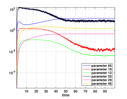
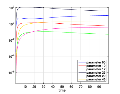
Figure 1: The instantaneous RE, defined in (15), for the EGFR model (left) and the averaged RE, defined in (32) (right).

Let us define a different sensitivity measure as the relative difference between the $k$-th species of two systems were the $\ell$-th parameter of the second is perturbed by $\epsilon^{\prime}$,

$$S_{k,\ell,t}:=\frac{X_{k,t}^{\theta}-X_{k,t}^{\theta+\epsilon_{\ell}}}{X_{k,t}^{\theta}}\ .$$ (33)

where $\epsilon_{\ell}$ is a vector with zeros everywhere and $\epsilon^{\prime}$ in the $\ell$-th position. In the following examples the value of $\epsilon^{\prime}$ for a perturbation in the $\ell$-th parameter is $\epsilon^{\prime}=0.1\theta_{\ell}$. By summing over all species we obtain a total sensitivity measure, which is only indexed by the parameter index and time,

$$S_{\ell,t}=\frac{1}{N}\sum_{k=1}^{N}S_{k,\ell,t}\ .$$ (34)

By observing the first row of Figure 2, which shows the instantaneous RE (16) for $\ell=10$ and $\ell=29$, we learn that perturbations in the $10$-th parameter have large sensitivity for small times and as time varies the sensitivity is getting smaller. On the other hand, perturbations in the $29$-th parameter have small influence on the system for small times while for larger times the sensitivity becomes significant. These observations are in good agreement with the sensitivity measure (35) presented in the second and third row of Figure 2.

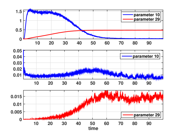
Figure 2: Instantaneous RE (15) for the EGFR model and parameters $10$ and $29$ (first row). The total sensitivity of the system, as defined in (34), due to perturbations in the $10$-th parameter (second row) and due to the $29$-th parameter (third row).

Moreover there is a crossing in the instantaneous RE which happens around $t=42$. After this time the sensitivity in parameter $\ell=29$ becomes more significant than the sensitivity in parameter $\ell=10$. This is again in agreement with the behavior of the sensitivity measure (35). This observation shows that the transient regime is more sensitive in perturbations in the $10$-th parameters while the equilibrium is more sensitive in perturbations in the $29$-th parameter.

7 Conclusions

In this paper we presented two pathwise sensitivity measures for the analysis of stochastic systems; the instantaneous relative entropy and its approximation, the instantaneous Fisher information matrix. These sensitivity tools serve as an extension to transient processes of the sensitivity tools presented in [13]. Three examples, discrete-time Markov chains, continuous-time Markov Chains and stochastic differential equations, were presented as an application of the new sensitivity measures. In Section 6 we demonstrated, in a biological reaction network, how the proposed pathwise sensitivity measure can be applied to transient, as well as in steady state regimes.

Finally, the pathwise sensitivity method is directly connected to a different sensitivity measure that depends on specific observables. More specifically, if we define the sensitivity index (SI) of the $\ell$-th observable to the $k$-th parameter as

$$S_{k,\ell}=\frac{\partial}{\partial\theta_{k}}\mathbb{E}\left[f_{\ell}\left(\{X_{s}\}_{s=0}^{T}\right)\right]\ ,$$ (35)

then IFIM (18) serves as un upper bound of $S_{k,\ell}$ through the inequality,

$$|S_{k,\ell}|\leq\sqrt{\mathrm{Var}_{Q_{0:T}^{\theta}}(f_{\ell})}\sqrt{{\mathcal{I}}\big{(}Q_{0:T}^{\theta}\big{)}_{k,k}}\ ,$$ (36)

where $F=(f_{1},...,f_{L})$ is a vector of observable functions. This inequality follows by rearranging the generalized Cramer-Rao bound for a biased estimator [30, 31]. Due to low variance of the estimator of IFIM compared to the variance of a finite difference estimator of $S_{k,\ell}$, the estimation of the right hand side of (36) is faster that that of the left hand side of (36). In [15] the authors use this inequality to efficiently screen out and exclude low sensitivity indices under a pre-specified value and then perform a coupling finite difference algorithm [8] to accurately estimate the remaining sensitivity indices $S_{k,\ell}$. In Figure 3 the estimated SIs for the EGFR model discussed in Section 6 are ordered in the parameter direction using only the IFIM (18). Notice that the SIs are then grouped into four distinct regions. For a detailed presentation of this methodology we refer to [15].

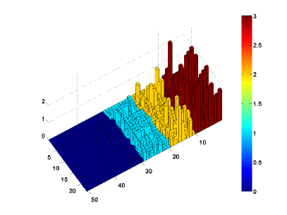
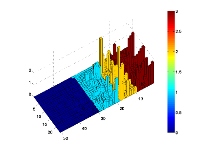
Figure 3: Ordering of the sensitivity index (35) in the time interval $[0,50]$ (left) and $[0,100]$ (right) utilizing the averaged IRE (32). In this case $f_{\ell}\left(\{X_{s}\}_{s=0}^{T}\right)=\frac{1}{T}\int_{0}^{T}X_{\ell,s}ds$ , which is the mean concentration of the $\ell$-th species in time interval $[0,T]$.

References

- [1] A. Saltelli, M. Ratto, T. Andres, F. Campolongo, J. Cariboni, D. Gatelli, M. Saisana, and S. Tarantola. Global Sensitivity Analysis. The Primer. Wiley, 2008.
- [2] J. DiStefano III. Dynamic Systems Biology Modeling and Simulation. Elsevier, 2013.
- [3] P.W. Glynn. Likelihood ratio gradient estimation for stochastic systems. Communications of the ACM, 33(10):75–84, 1990.
- [4] M. Nakayama, A. Goyal, and P. W. Glynn. Likelihood ratio sensitivity analysis for Markovian models of highly dependable systems. Stochastic Models, 10:701–717, 1994.
- [5] S. Plyasunov and A. P. Arkin. Efficient stochastic sensitivity analysis of discrete event systems. J. Comp. Phys., 221:724–738, 2007.
- [6] D. Kim, B.J. Debusschere, and H.N. Najm. Spectral methods for parametric sensitivity in stochastic dynamical systems. Biophysical Journal, 92:379–393, 2007.
- [7] M. Rathinam, P. W. Sheppard, and M. Khammash. Efficient computation of parameter sensitivities of discrete stochastic chemical reaction networks. J. Chem. Phys., 132:034103–(1–13), 2010.
- [8] David F. Anderson. An efficient finite difference method for parameter sensitivities of continuous-time Markov chains. SIAM J. Numerical Analysis, 50(5):2237–2258, 2012.
- [9] P.W. Sheppard, M. Rathinam, and M. Khammash. A pathwise derivative approach to the computation of parameter sensitivities in discrete stochastic chemical systems. J. Chem. Phys., 136(3):034115, 2012.
- [10] H. Meskine, S. Matera, M. Scheffler, K. Reuter, and H. Metiu. Examination of the concept of degree of rate control by first-principles kinetic Monte Carlo simulations. Surf. Science, 603(10-12):1724–1730, 2009.
- [11] C. Maes M. Baiesi and B. Wynants. Nonequilibrium linear response for markov dynamics, i: jump processes and overdamped diffusions. J. Stat. Phys., 2009.
- [12] E. Boksenbojm M. Baiesi, C. Maes and B. Wynants. Nonequilibrium linear response for markov dynamics, ii: Inertial dynamics. J. Stat. Phys., 2010.
- [13] Y. Pantazis and M. Katsoulakis. A relative entropy rate method for path space sensitivity analysis of stationary complex stochastic dynamics. J. Chem. Phys., 138(5):054115, 2013.
- [14] P. Dupuis, M.A. Katsoulakis, Y. Pantazis, and P. Plecháč. Sesnitivity bounds and error estimates for stochastic models. (in preparation).
- [15] G. Arampatzis and Y. Pantazis M. A. Katsoulakis. Accelerated sensitivity analysis in high-dimensional stochastic reaction networks. Submitted to PLoS ONE.
- [16] S. Kullback. Information theory and statistics. John Wiley and Sons, NY, 1959.
- [17] T. Cover and J. Thomas. Elements of Information Theory. John Wiley & Sons, 1991.
- [18] C. Kipnis and C. Landim. Scaling Limits of Interacting Particle Systems. Springer-Verlag, 1999.
- [19] M. Avellaneda, C.A. Friedman, R. Holmes, and D.J. Samperi. Calibrating volatility surfaces via relative-entropy minimization. Social Science Research Network, 1997.
- [20] HB Liu, W Chen, and A Sudjianto. Relative entropy based method for probabilistic sensitivity analysis in engineering design. J. Mechanical Design, 128:326–336, 2006.
- [21] N. Limnios and G. Oprisan. Semi-Markov Processes and Reliability. Springer, 2001.
- [22] R. V. Abramov, M. J. Grote, and A. J. Majda. Information Theory and Stochastics for Multiscale Nonlinear Systems. CRM Monograph Series, 2005.
- [23] R. S. Liptser and A. N. Shiryaev. Statistics of Random Processes: I & II. Springer, 1977.
- [24] B Oksendal. Stochastic Differential Equations: An introduction with applications. Springer-Verlag, 2000.
- [25] A. Tsourtis, Y. Pantazis, and V. Harmandaris M.A. Katsoulakis. Parametric sensitivity analysis for stochastic molecular systems using information theoretic metrics. Submitted to J of Chemical Physics.
- [26] Boris N Kholodenko, Oleg V Demin, Gisela Moehren, and Jan B Hoek. Quantification of short term signaling by the epidermal growth factor receptor. Journal of Biological Chemistry, 274(42):30169–30181, 1999.
- [27] N. Moghal and P.W. Sternberg. Multiple positive and negative regulators of signaling by the egf receptor. Curr. Opin. Cell. Biol., 11:190–196, 1999.
- [28] P.O. Hackel, E. Zwick, N. Prenzel, and A. Ullrich. Epidermal growth factor receptors: critical mediators of multiple receptor pathways. Curr. Opin. Cell. Biol., 11:184–189, 1999.
- [29] B. Schoeberl, C. Eichler-Jonsson, E.D. Gilles, and G. Muller. Computational modeling of the dynamics of the MAP kinase cascade activated by surface and internalized EGF receptors. Nature Biotechnology, 20:370–375, 2002.
- [30] G. Casella and R.L. Berger. Statistical Inference. Duxbury advanced series in statistics and decision sciences. Thomson Learning, 2002.
- [31] S. M. Kay. Funtamentals of Statistical Signal Processing: Estimation Theory. Prentice-Hall, Englewood Cliffs, NJ, 1993.