SLUG – Stochastically Lighting Up Galaxies. III: A Suite of Tools for Simulated Photometry, Spectroscopy, and Bayesian Inference with Stochastic Stellar Populations
Abstract
Stellar population synthesis techniques for predicting the observable light emitted by a stellar population have extensive applications in numerous areas of astronomy. However, accurate predictions for small populations of young stars, such as those found in individual star clusters, star-forming dwarf galaxies, and small segments of spiral galaxies, require that the population be treated stochastically. Conversely, accurate deductions of the properties of such objects also requires consideration of stochasticity. Here we describe a comprehensive suite of modular, open-source software tools for tackling these related problems. These include: a greatly-enhanced version of the slug code introduced by da Silva et al. (2012), which computes spectra and photometry for stochastically- or deterministically-sampled stellar populations with nearly-arbitrary star formation histories, clustering properties, and initial mass functions; cloudy_slug, a tool that automatically couples slug-computed spectra with the cloudy radiative transfer code in order to predict stochastic nebular emission; bayesphot, a general-purpose tool for performing Bayesian inference on the physical properties of stellar systems based on unresolved photometry; and cluster_slug and SFR_slug, a pair of tools that use bayesphot on a library of slug models to compute the mass, age, and extinction of mono-age star clusters, and the star formation rate of galaxies, respectively. The latter two tools make use of an extensive library of pre-computed stellar population models, which are included the software. The complete package is available at http://www.slugsps.com.
keywords:
methods: statistical; galaxies: star clusters: general; galaxies: stellar content; stars: formation; methods: numerical; techniques: photometric1 Introduction
Stellar population synthesis (SPS) is a critical tool that allows us to link the observed light we receive from unresolved stellar populations to the physical properties (e.g. mass, age) of the emitting stars. Reflecting this importance, over the years numerous research groups have written and distributed SPS codes such as starburst99 (Leitherer et al., 1999; Vázquez & Leitherer, 2005), fsps (Conroy et al., 2009; Conroy & Gunn, 2010), pegase (Fioc & Rocca-Volmerange, 1997), and galaxev (Bruzual & Charlot, 2003). All these codes perform essentially the same computation. One adopts a star formation history (SFH) and an initial mass function (IMF) to determine the present-day distribution of stellar masses and ages. Next, using a set of stellar evolutionary tracks and atmospheres that give the luminosity (either frequency-dependent or integrated over some filter) for a star of a particular mass and age, one integrates the stellar luminosity weighted by the age and mass distributions. These codes differ in the range of functional forms they allow for the IMF and SFH, and the evolutionary tracks and model atmospheres they use, but the underlying computation is much the same in all of them. While this approach is adequate for many applications, it fails for systems with low masses and star formation rates (SFRs) because it implicitly assumes that the stellar mass and age distributions are well-sampled. This is a very poor assumption both in star-forming dwarf galaxies and in resolved segments of larger galaxies.
Significantly less work has been done in extending SPS methods to the regime where the IMF and SFH are not well-sampled. There are a number of codes available for simulating a simple stellar population (i.e., one where all the stars are the same age, so the SFH is described by a distribution) where the IMF is not well sampled (Maíz Apellániz, 2009; Popescu & Hanson, 2009, 2010b, 2010a; Fouesneau & Lançon, 2010; Fouesneau et al., 2012; Fouesneau et al., 2014; Anders et al., 2013; de Meulenaer et al., 2013, 2014, 2015), and a great deal of analytic work has also been performed on this topic (Cerviño & Valls-Gabaud, 2003; Cerviño & Luridiana, 2004, 2006) – see Cerviño (2013) for a recent review. However, these codes only address the problem of stochastic sampling of the IMF; for non-simple stellar populations, stochastic sampling of the SFH proves to be a more important effect (Fumagalli et al., 2011; da Silva et al., 2014).
To handle this problem, we introduced the stochastic SPS code slug (da Silva et al., 2012), which includes full stochasticity in both the IMF and the SFH. Crucially, slug properly handles the clustered nature of star formation (e.g., Lada & Lada, 2003; Krumholz, 2014). This has two effects. First, clustering itself can interact with IMF sampling so that the total mass distribution produced by a clustered population is not identical to that of a non-clustered population drawn from the same underlying IMF. Second and perhaps more importantly, clustering causes large short-timescale fluctuations in the SFR even in galaxies whose mean SFR averaged over longer timescales is constant. Since its introduction, this code has been used in a number of applications, including explaining the observed deficit of H emission relative to FUV emission in dwarf galaxies (Fumagalli et al., 2011; Andrews et al., 2013, 2014), quantifying the stochastic uncertainties in SFR indicators (da Silva et al., 2014), analyzing the properties of star clusters in dwarf galaxies in the ANGST survey (Cook et al., 2012), and analyzing Lyman continuum radiation from high-redshift dwarf galaxies (Forero-Romero & Dijkstra, 2013). The need for a code with stochastic capabilities is likely to increase in the future, as studies of local galaxies such as PHAT (Dalcanton et al., 2012), HERACLES (Leroy et al., 2013), and LEGUS (Calzetti et al., 2015), and even studies in the high redshift universe (e.g., Jones et al., 2013a, b) increasingly push to smaller spatial scales and lower rates of star formation, where stochastic effects become increasingly important.
In this paper we describe a major upgrade and expansion of slug, intended to make it a general-purpose solution for the analysis of stochastic stellar populations. This new version of slug allows essentially arbitrary functional forms for both the IMF and the SFH, allows a wide range of stellar evolutionary tracks and atmosphere models, and can output both spectroscopy and photometry in a list of filters. It can also include the effects of reprocessing of the light by interstellar gas and by stochastically-varying amounts of dust, and can interface with the cloudy photoionization code (Ferland et al., 2013) to produce predictions for stochastically-varying nebular emission. Finally, we have coupled slug to a new set of tools for solving the “inverse problem” in stochastic stellar population synthesis: given a set of observed photometric properties, infer the posterior probability distribution for the properties of the underlying stellar population, in the case where the mapping between such properties and the photometry is stochastic and therefore non-deterministic (e.g. da Silva et al., 2014). The full software suite is released under the GNU Public License, and is freely available from http://www.slugsps.com.111As of this writing http://www.slugsps.com is hosted on Google Sites, and thus is inaccessible from mainland China. Chinese users can access the source code from https://bitbucket.org/krumholz/slug2, and should contact the authors by email for the ancillary data products.
In the remainder of this paper, we describe slug and its companion software tools in detail (Section 2), and then provide a series of demonstrations of the capabilities of the upgraded version of the code (Section 3). We end with a summary and discussion of future prospects for this work (Section 4).
2 The SLUG Software Suite
The slug software suite is a collection of tools designed to solve two related problems. The first is to determine the probability distribution function (PDF) of observable quantities (spectra, photometry, etc.) that are produced by a stellar population characterized by a specified set of physical parameters (IMF, SFH, cluster mass function, and an array of additional ancillary inputs). This problem is addressed by the core slug code (Section 2.1) and its adjunct cloudy_slug (Section 2.2), which perform Monte Carlo simulations to calculate the distribution of observables. The second problem is to use those PDFs to solve the inverse problem: given a set of observed properties, what should we infer about the physical properties of the stellar population producing those observables? The bayesphot package provides a general solution to this problem (Section 2.3), and the SFR_slug and cluster_slug packages specialize this general solution to the problem of inferring star formation rates for continuously star-forming galaxies, and masses, ages, and extinctions from simple stellar populations, respectively (Section 2.4). The entire software suite is available from http://www.slugsps.com, and extensive documentation is available at http://slug2.readthedocs.org/en/latest/.
2.1 slug: A Highly Flexible Tool for Stochastic Stellar Population Synthesis
The core of the software suite is the stochastic stellar population synthesis code slug. The original slug code is described in da Silva et al. (2012), but the code described here is a complete re-implementation with greatly expanded capabilities. The code operates in two main steps; first it generates the spectra from the stellar population (Section 2.1.1) and then it post-processes the spectra to include the effects of nebular emission and dust absorption, and to produce photometric predictions as well as spectra (Section 2.1.2). In this section we limit ourselves to a top-level description of the physical model, and provide some more details on the numerical implementation in Appendices A, B, and C.
2.1.1 Generating the Stellar Population
Slug can simulate both simple stellar populations (SSPs, i.e., ones where all the stars are coeval) and composite ones. We begin by describing the SSP model, since composite stellar populations in slug are built from collections of SSPs. For an SSP, the stellar population is described by an age, a total mass, and an IMF. Slug allows nearly-arbitrary functional forms for the IMF, and is not restricted to a set of predetermined choices; see Appendix A.1 for details.
In non-stochastic SPS codes, once an age, mass, and IMF are chosen, the standard procedure is to use a set of stellar tracks and atmospheres to predict the luminosity (either frequency-dependent, or integrated over a specified filter) as a function of stellar mass and age, and to integrate the mass-dependent luminosity multiplied by the stellar mass distribution to compute the output spectrum at a specified age. Slug adds an extra step: instead of evaluating an integral, it directly draws stars from the IMF until the desired total mass has been reached. As emphasized by a number of previous authors (e.g. Weidner & Kroupa, 2006; Haas & Anders, 2010; Cerviño, 2013; Popescu & Hanson, 2014), when drawing a target mass rather than a specified number of objects from a PDF, one must also choose a sampling method to handle the fact that, in general, it will not be possible to hit the target mass exactly. Many sampling procedures have been explored in the literature, and slug provides a large number of options, as described in Appendix A.1.
Once a set of stars is chosen, slug proceeds much like a conventional SPS code. It uses a chosen set of tracks and atmospheres to determine the luminosity of each star, either wavelength-dependent or integrated over one or more photometric filters, at the specified age. It then sums over all stars to determine the integrated light output. Details of the available sets of tracks and atmospheres, and slug’s method for interpolating them, are provided in Appendix A.2.
Composite stellar populations in slug consist of a collection of “star clusters”, each consisting of an SSP, plus a collection of “field stars” whose ages are distributed continuously. In practice, this population is described by four parameters beyond those that describe SSPs: the fraction of stars formed in clusters as opposed to the field , the cluster mass function (CMF), cluster lifetime function (CLF), and star formation history (SFH). As with the IMF, the latter three are distributions, which can be specified using nearly arbitrary functional forms and a wide range of sampling methods as described in Appendix A.1. For a simulation with a composite stellar population, slug performs a series of steps: (1) at each user-requested output time222Slug can either output results at specified times, or the user can specify a distribution from which the output time is to be drawn. The latter capability is useful when we wish to sample a distribution of times continuously so that the resulting data set can be used to infer ages from observations – see Section 2.4., slug uses the SFH and the cluster fraction to compute the additional stellar mass expected to have formed in clusters and out of clusters (in “the field”) since the previous output; (2) for the non-clustered portion of the star formation, slug draws the appropriate mass in individual stars from the IMF, while for the clustered portion it draws a cluster mass from the CMF, and then it fills each cluster with stars drawn from the IMF; (3) each star and star cluster formed is assigned an age between the current output and the previous one, selected to produce a realisation of the input SFH333One subtlety to note here is that the choice of output grid can produce non-trivial modifications of the statistical properties of the output in cases where the expected mass of stars formed is much smaller than the maximum possible cluster mass. For example, consider a simulation with a constant SFR and an output grid chosen such that the expected mass of stars formed per output time is . If the sampling method chosen is STOP_NEAREST (see Appendix A.1), the number of clusters formed will typically be smaller than if the same SFH were used but the outputs were spaced 100 times further apart, giving an expected mass of between outputs.; (4) each cluster that is formed is assigned a lifetime drawn from the CLF, which is the time at which the cluster is considered dispersed.
The end result of this procedure is that, at each output time, slug has constructed a “galaxy” consisting of a set of star clusters and field stars, each with a known age. Once the stellar population has been assembled, the procedure for determining spectra and photometry is simply a sum over the various individual simple populations. In addition to computing the integrated spectrum of the entire population, slug can also report individual spectra for each cluster that has not disrupted (i.e., where the cluster age is less than the value drawn from the CLF for that cluster). Thus the primary output consists of an integrated monochromatic luminosity for the entire stellar population, and a value for the th remaining cluster, at each output time.
Finally, we note that slug is also capable of skipping the sampling procedure and evaluating the light output of stellar populations by integrating over the IMF and SFH, exactly as in a conventional, non-stochastic SPS code. In this case, slug essentially emulates starburst99 (Leitherer et al., 1999; Vázquez & Leitherer, 2005), except for subtle differences in the interpolation and numerical integration schemes used (see Appendix A.2). Slug can also behave “semi-stochastically”, evaluating stars’ contribution to the light output using integrals to handle the IMF up to some mass, and using stochastic sampling at higher masses.
2.1.2 Post-Processing the Spectra
Once slug has computed a spectrum for a simple or composite stellar population, it can perform three additional post-processing steps. First, it can provide an approximate spectrum after the starlight has been processed by the surrounding H ii region. In this case, the nebular spectrum is computed for an isothermal, constant-density H ii region, within which it is assumed that He is all singly-ionized. Under these circumstances, the photoionized volume , electron density , and hydrogen density obey the relation
| (1) |
where
| (2) |
is the hydrogen-ionizing luminosity, is the luminosity per unit frequency, eV is the ionization potential of neutral hydrogen, , is the He abundance relative to hydrogen (assumed to be 0.1), is the fraction of H-ionizing photons that are absorbed by hydrogen atoms within the H ii region rather than escaping or being absorbed by dust, and is the temperature-dependent case B recombination coefficient. The nebular luminosity can then be written as
| (3) |
where is the wavelength-dependent nebular emission coefficient. Our calculation of this quantity includes the following processes: free-free and bound-free emission arising from electrons interacting with H+ and He+, two-photon emission from neutral hydrogen in the state, H recombination lines, and non-H lines computed approximately from tabulated values. Full details on the method by which we perform this calculation are given in Appendix B. The composite spectrum after nebular processing is zero at wavelength shorter than 912 Å (corresponding to the ionization potential of hydrogen), and the sum of intrinsic stellar spectrum and the nebular spectrum at longer wavelengths. Slug reports this quantity both cluster-by-cluster and for the galaxy as a whole.
Note that the treatment of nebular emission included in slug is optimized for speed rather than accuracy, and will produce significantly less accurate results than cloudy_slug (see Section 2.2). The major limitations of the built-in approach are: (1) because slug’s built-in calculation relies on pre-tabulated values for the metal line emission and assumes either a constant or a similarly pre-tabulated temperature (which significantly affects the continuum emission), it misses the variation in emission caused by the fact that H ii regions exist at a range of densities and ionization parameters, which in turn induces substantial variations in their nebular emission (e.g. Yeh et al., 2013; Verdolini et al., 2013); (2) slug’s built-in calculation assumes a uniform density H ii region, an assumption that will fail at high ionizing luminosities and densities due to the effects of radiation pressure (Dopita et al., 2002; Krumholz et al., 2009; Draine, 2011; Yeh & Matzner, 2012; Yeh et al., 2013); (3) slug’s calculation correctly captures the effects of stochastic variation in the total ionizing luminosity, but it does not capture the effects of variation in the spectral shape of the ionizing continuum, which preliminary testing suggests can cause variations in line luminosities at the few tenths of a dex level even for fixed total ionizing flux. The reason for accepting these limitations is that the assumptions that cause them also make it possible to express the nebular emission in terms of a few simple parameter that can be pre-tabulated, reducing the computational cost of evaluating the nebular emission by orders of magnitude compared to a fully accurate calculation with cloudy_slug.
The second post-processing step available is that slug can apply extinction in order to report an extincted spectrum, both for the pure stellar spectrum and for the nebula-processed spectrum. Extinction can be either fixed to a constant value for an entire simulation, or it can be drawn from a specified PDF. In the latter case, for simulations of composite stellar populations, every cluster will have a different extinction. More details are given in Appendix B.
As a third and final post-processing step, slug can convolve all the spectra it computes with one or more filter response functions in order to predict photometry. Slug includes the large list of filter response functions maintained as part of FSPS (Conroy et al., 2010; Conroy & Gunn, 2010), as well as a number of Hubble Space Telescope filters444These filters were downloaded from http://www.stsci.edu/~WFC3/UVIS/SystemThroughput/ and http://www.stsci.edu/hst/acs/analysis/throughputs for the UVIS and ACS instruments, respectively. not included in FSPS; at present, more than 130 filters are available. As part of this calculation, slug can also output the bolometric luminosity, and the photon luminosity in the H0, He0, and He+ ionizing continua.
2.2 cloudy_slug: Stochastic Nebular Line Emission
In broad outlines, the cloudy_slug package is a software interface that automatically takes spectra generated by slug and uses them as inputs to the cloudy radiative transfer code (Ferland et al., 2013). Cloudy_slug then extracts the continuous spectra and lines returned by cloudy, convolves them with the same set of filters as in the original slug calculation in order to predict photometry. The user can optionally also examine all of cloudy’s detailed outputs. As with the core slug code, details on the software implementation are given in Appendix C.
When dealing with composite stellar populations, calculating the nebular emission produced by a stellar population requires making some physical assumptions about how the stars are arranged, and cloudy_slug allows two extreme choices that should bracket reality. One extreme is to assume that all stars are concentrated in a single point of ionizing radiation at the center of a single H ii region. We refer to this as integrated mode, and in this mode the only free parameters to be specified by a user are the chemical composition of the gas into which the radiation propagates and its starting density.
The opposite assumption, which we refer to as cluster mode, is that every star cluster is surrounded by its own H ii region, and that the properties of these regions are to be computed individually using the stellar spectrum of each driving cluster and only then summed to produce a composite output spectrum. At present cluster mode does not consider contributions to the nebular emission from field stars, and so should not be used when the cluster fraction . In the cluster case, the H ii regions need not all have the same density or radius; indeed, one would expect a range of both properties to be present, since not all star clusters have the same age or ionizing luminosity. We handle this case using a simplified version of the H ii population synthesis model introduced by Verdolini et al. (2013) and Yeh et al. (2013). The free parameters to be specified in this model are the chemical composition and the density in the ambient neutral ISM around each cluster. For an initially-neutral region of uniform hydrogen number density , the radius of the H ii at a time after it begins expanding is well-approximated by (Krumholz & Matzner, 2009)
| (4) | |||||
| (5) | |||||
| (6) | |||||
| (7) | |||||
| (8) | |||||
| (9) |
where cm3 s-1 is the case B recombination coefficient at K, is the typical H ii region temperature, is a trapping factor that accounts for stellar wind and trapped infrared radiation pressure, is the mean photon energy in Rydberg for a fully sampled IMF at zero age555This value of is taken from Murray & Rahman (2010), and is based on a Chabrier (2005) IMF and a compilation of empirically-measured ionizing luminosities for young stars. However, alternative IMFs and methods of computing the ionizing luminosity give results that agree to tens of percent., and is the mean mass per hydrogen nucleus for gas with the usual helium abundance . The solution includes the effects of both radiation and gas pressure in driving the expansion. Once the radius is known, the density near the H ii region center (the parameter required by cloudy) can be computed from the usual ionization balance argument,
| (10) |
Note that the factor of in the denominator accounts for the extra free electrons provided by helium, assuming it is singly ionized. Also note that this will not give the correct density during the brief radiation pressure-dominated phase early on in the evolution, but that this period is very brief (though the effects of the extra boost provided by radiation pressure can last much longer), and no simple analytic approximation for this density is available (Krumholz & Matzner, 2009). Also note that, although cloudy_slug presently only supports this parameterization of H ii region radius and density versus time, the code is simply a python script. It would therefore be extremely straightforward for a user who prefers a different parameterization to alter the script to supply it.
In cluster mode, cloudy_slug uses the approximation described above to compute the density of the ionized gas in the vicinity of each star cluster, which is then passed as an input to cloudy along with the star cluster’s spectrum. Note that computations in cluster mode are much more expensive than those in integrated mode, since the latter requires only a single call to cloudy per time step, while the former requires one per cluster. To ease the computational requirements slightly, in cluster mode one can set a threshold ionizing luminosity below which the contribution to the total nebular spectrum is assumed to be negligible, and is not computed.
2.3 bayesphot: Bayesian Inference from Stellar Photometry
2.3.1 Description of the Method
Simulating stochastic stellar populations is useful, but to fully exploit this capability we must tackle the inverse problem: given an observed set of stellar photometry, what should we infer about the physical properties of the underlying stellar population in the regime where the mapping between physical and photometric properties is non-deterministic? A number of authors have presented numerical methods to tackle problems of this sort, mostly in the context of determining the properties of star clusters with stochastically-sampled IMFs (Popescu & Hanson, 2009, 2010b, 2010a; Fouesneau & Lançon, 2010; Fouesneau et al., 2012; Popescu et al., 2012; Asa’d & Hanson, 2012; Anders et al., 2013; de Meulenaer et al., 2013, 2014, 2015), and in some cases in the context of determining SFRs from photometry (da Silva et al., 2014). Our method here is a generalization of that developed in da Silva et al. (2014), and has a number of advantages as compared to earlier methods, both in terms of its computational practicality and its generality.
Consider stellar systems characterized by a set of physical parameters ; in the example of star clusters below we will have , with , , and representing the logarithm of the mass, the logarithm of the age, and the extinction, while for galaxies forming stars at a continuous rate we will have , with representing the logarithm of the SFR. The light output of these systems is known in photometric bands; let be a set of photometric values, for example magnitudes in some set of filters. Suppose that we observe a stellar population in these bands and measure a set of photometric values , with some errors , which for simplicity we will assume are Gaussian. We wish to infer the posterior probability distribution for the physical parameters given the observed photometry and photometric errors, .
Following da Silva et al. (2014), we compute the posterior probability via implied conditional regression coupled to kernel density estimation. Let the joint PDF of physical and photometric values for the population of all the stellar populations under consideration be . We can write the posterior probability distribution we seek as
| (11) |
where is the distribution of the photometric variables alone, i.e.,
| (12) |
If we have an exact set of photometric measurements , with no errors, then the denominator in equation (11) is simply a constant that will normalize out, and the posterior probability distribution we seek is distributed simply as
| (13) |
In this case, the problem of computing reduces to that of computing the joint physical-photometric PDF at any given set of observed photometric values .
For the more general case where we do have errors, we first note that the posterior probability distribution for the true photometric value is given by the prior probability distribution for photometric values multiplied by the likelihood function associated with our measurements. The prior PDF of photometric values is simply as given by equation (12), and for a central observed value of with errors , the likelihood function is simply a Gaussian. Thus the PDF of given our observations is
| (14) |
where
| (15) |
is the usual multi-dimensional Gaussian function. The posterior probability for the physical parameters is then simply the convolution of equations (11) and (14), i.e.,
| (16) | |||||
Note that we recover the case without errors, equation (13), in the limit where , because in that case the Gaussian .
We have therefore reduced the problem of computing to that of computing , the joint PDF of physical and photometric parameters, for our set of stellar populations. To perform this calculation, we use slug to create a large library of models for the type of stellar population in question. We draw the physical properties of the stellar populations (e.g., star cluster mass, age, and extinction) in our library from a distribution , and for each stellar population in the library we have a set of physical and photometric parameters and . We estimate using a kernel density estimation technique. Specifically, we approximate this PDF as
| (17) |
where is the weight we assign to sample , is our kernel function, is our bandwidth parameter (see below), and the sum runs over every simulation in our library. We assign weights to ensure that the distribution of physical parameters matches whatever prior probability distributions we wish to assign for them. If we let represent our priors, then this is
| (18) |
Note that, although we are free to choose and thus weight all samples equally, it is often advantageous for numerical or astrophysical reasons not to do so, because then we can distribute our sample points in a way that is chosen to maximize our knowledge of the shape of with the fewest possible realizations. As a practical example, we know that photometric outputs will fluctuate more for galaxies with low star formation rates than for high ones, so the library we use for SFR_slug (see below) is weighted to contain more realizations at low than high SFR.
We choose to use a Gaussian kernel function, , because this presents significant computational advantages. Specifically, with this choice, equation (16) becomes
| (20) | |||||
| (21) | |||||
where is the bandwidth in the physical dimensions, is the bandwidth in the photometric dimensions, and the quadrature sum is understood to be computed independently over every index in and . The new quantity we have introduced,
| (22) |
is simply a modified bandwidth in which the bandwidth in the photometric dimensions has been broadened by adding the photometric errors in quadrature sum with the bandwidths in the corresponding dimensions. Note that, in going from equation (20) to equation (20) we have invoked the result that the convolution of two Gaussians is another Gaussian, whose width is the quadrature sum of the widths of the two input Gaussians, and whose center is located at the difference between the two input centers.
As an adjunct to this result, we can also immediately write down the marginal probabilities for each of the physical parameters in precisely the same form. The marginal posterior probability distribution for is simply
| (24) | |||||
and similarly for all other physical variables. This expression also immediately generalizes to the case of joint marginal probabilities of the physical variables. We have therefore succeeded in writing down the posterior probability distribution for all the physical properties, and the marginal posterior distributions of any of them individually or in combination, via a kernel density estimation identical to that given by equation (17). One advantage of equations (21) and (24) is that they are easy to evaluate quickly using standard numerical methods. Details on our software implementation are given in Appendix C.
2.3.2 Error Estimation and Properties of the Library
An important question for bayesphot, or any similar method, is how large a library must be in order to yield reliable results. Of course this depends on what quantity is being estimated and on the shape of the underlying distribution. Full, rigorous, error analysis is best accomplished by bootstrap resampling. However, we can, without resorting to such a computationally-intensive procedure, provide a useful rule of thumb for how large a library must be so that the measurements rather than the library are the dominant source of uncertainty in the resulting derived properties.
Consider a library of simulations, from which we wish to measure the value that delineates a certain quantile (i.e., the percentile ) of the underlying distribution from which the samples are drawn. Let for be the samples in our library, ordered from smallest to largest. Our central estimate for the value of that delineates quintile , will naturally be . (Throughout this argument we will assume that is large enough that we need not worry about the fact that ranks in the list, such as , will not exactly be integers. Extending this argument to include the necessary continuity correction adds mathematical complication but does not change the basic result.) For example, we may have a library of simulations of galaxies at a particular SFR (or in a particular interval of SFRs), and wish to know what ionizing luminosity corresponds to the 95th percentile at that SFR. Our estimate for the 95th percentile ionizing luminosity will simply be the ionizing luminosity of the 950,000th simulation in the library.
To place confidence intervals around this estimate, note that the probability that a randomly chosen member of the population will have a value is , and conversely the probability that is . Thus in our library of simulations, the probability that we have exactly samples for which is given by the binomial distribution,
| (25) |
When , , and , the binomial distribution approaches a Gaussian distribution of central value and standard deviation :
| (26) |
That is, the position in our library of simulations such that for all , and for all , is distributed approximately as a Gaussian, centered at , with dispersion . This makes it easy to compute confidence intervals on , because it reduces the problem that of computing confidence intervals on a Gaussian. Specifically, if we wish to compute the central value and confidence interval (e.g., is the 68% confidence interval) for the rank corresponding to percentile , this is
| (27) |
The corresponding central value for (as opposed to its rank in the list) is , and the confidence interval is
| (28) |
In our example of determining the 95th percentile from a library of simulations, our central estimate of this value is the , the 950,000th simulation in the library, and the 90% confidence interval is 359 ranks on either side of this. That is, our 90% confidence interval extends from to .
This method may be used to define confidence intervals on any quantile derived from a library of slug simulations. Of course this does not specifically give confidence intervals on the results derived when such a library is used as the basis of a Bayesian inference from bayesphot. However, this analysis can still provide a useful constraint: the error on the values derived from bayesphot cannot be less than the errors on the underlying photometric distribution we have derived from the library. Thus if we have a photometric measurement that lies at the th quantile of the library we are using for kernel density estimation in bayesphot, the effective uncertainty our kernel density estimation procedure provides is at a minimum given by the uncertainty in the quantile value calculated via the procedure above. If this uncertainty is larger than the photometric uncertainties in the measurement, then the resolution of the library rather than the accuracy of the measurement will be the dominant source of error.
2.4 sfr_slug and cluster_slug: Bayesian Star Formation Rates and Star Cluster Properties
The slug package ships with two Bayesian inference modules based on bayesphot. SFR_slug, first described in da Silva et al. (2014) and modified slightly to use the improved computational technique described in the previous section, is a module that infers the posterior probability distribution of the SFR given an observed flux in H, GALEX FUV, or bolometric luminosity, or any combination of the three. The library of models on which it operates (which is included in the slug package) consists of approximately galaxies with constant SFRs sampling a range from yr-1, with no extinction; the default bandwidth is 0.1 dex. We refer readers for da Silva et al. (2014) for a further description of the model library. SFR_slug can download the default library automatically, and it is also available as a standalone download from http://www.slugsps.com/data.
The cluster_slug package performs a similar task for inferring the mass, age, and extinction of star clusters. The slug models that cluster_slug uses consist of libraries of simple stellar populations with masses in the range , ages , and extinctions mag. The maximum age is either 1 Gyr or 15 Gyr, depending on the choice of tracks (see below). The data are sampled uniformly in . In mass the library sampling is for masses up to , and as at higher masses; similarly, the library age sampling is for yr, and as at older ages. The motivation for this sampling is that it puts more computational effort at younger ages and low masses, where stochastic variation is greatest. The libraries all use a Chabrier (2005) IMF, and include nebular emission computed using and an ionization parameter (see Appendix B). Libraries are available using either Padova or Geneva tracks, with the former having a maximum age of 15 Gyr and the latter a maximum age of 1 Gyr. The Geneva tracks are available using either Milky Way or “starburst” extinction curves (see Appendix B). The default bandwidth is 0.1 dex in mass and age, 0.1 mag in extinction, and 0.25 mag (corresponding to 0.1 dex in luminosity) in photometry. For each model, photometry is computed for a large range of filters, listed in Table 1. As with SFR_slug, cluster_slug can automatically download the default library, and the data are also available as a standalone download from http://www.slugsps.com/data. Full spectra for the library, allowing the addition of further filters as needed, are also available upon request; they are not provided for web download due to the large file sizes involved.
| Type | Filter Name |
|---|---|
| HST WFC3 UVIS wide | F225W, F275W, F336W, F360W, F438W, F475W, F555W, F606W, F775W, F814W |
| HST WFC3 UVIS medium/narrow | F547M, F657N, F658N |
| HST WFC3 IR | F098M, F105W, F110W, F125W, F140W, F160W |
| HST ACS wide | F435W, F475W, F555W, F606W, F625W, F775W, F814W |
| HST ACS medium/narrow | F550M, F658N, F660N |
| HST ACS HRC | F330W |
| HST ACS SBC | F125LP, F140LP, F150LP F165LP |
| Spitzer IRAC | 3.6, 4.5, 5.8, 8.0 |
| GALEX | FUV, NUV |
| Johnson-Cousins | U, B, V, R, I |
| SDSS | u, g, r, i, z |
| 2MASS | J, H, Ks |
3 Sample Applications
In this section, we present a suite of test problems with the goal of illustrating the
different capabilities of slug, highlighting the effects of key parameters on slug’s simulations,
and validating the code. Unless otherwise stated, all computations use the Geneva (2013) non-rotating
stellar tracks and stellar atmospheres following the starburst99 implementation.
3.1 Sampling Techniques
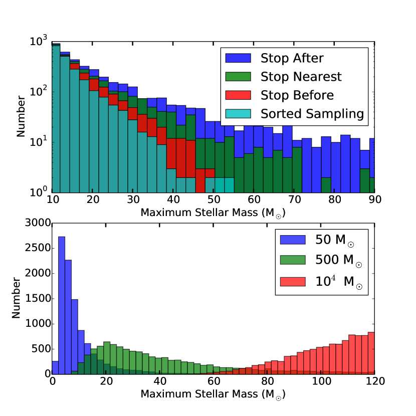
As discussed above and in the literature (e.g., Weidner & Kroupa, 2006; Haas & Anders, 2010; da Silva et al., 2012; Cerviño et al., 2013; Popescu & Hanson, 2014), the choice of sampling technique used to generate stellar masses can have significant effects on the distribution of stellar masses and the final light output, even when the underlying distribution being sampled is held fixed. This can have profound astrophysical implications. Variations in sampling technique even for a fixed IMF can produce systematic variations in galaxy colors (e.g., Haas & Anders, 2010), nucleosynthetic element yields (e.g., Köppen et al., 2007; Haas & Anders, 2010), and observational tracers of the star formation rate (e.g., Weidner et al., 2004; Pflamm-Altenburg et al., 2007). It is therefore of interest to explore how sampling techniques influence various aspects of stellar populations. We do so as a first demonstration of slug’s capabilities. Here we consider the problem of populating clusters with stars from an IMF, but our discussion also applies to the case of “galaxy” simulations. Specifically, we run four sets of “cluster” simulations with a target mass of 50 M⊙ by sampling a Kroupa (2002) IMF with the STOP_NEAREST, STOP_AFTER, STOP_BEFORE, SORTED_SAMPLING conditions (see Appendix A.1). In the following, we analyse a single timestep at yr.
By default, slug adopts the STOP_NEAREST condition, according to which the final draw from the IMF is added to the cluster only if the inclusion of this last star minimises the absolute error between the target and the achieved cluster mass. In this case, the cluster mass sometimes exceeds and sometimes falls short of the desired mass. The STOP_AFTER condition, instead, always includes the final draw from the IMF. Thus, with this choice, slug simulations produce clusters with masses that are always in excess of the target mass. The opposite behaviour is obviously recovered by the STOP_BEFORE condition, in which the final draw is always rejected. Finally, for SORTED_SAMPLING condition, the final cluster mass depends on the details of the chosen IMF.
Besides this manifest effect of the sampling techniques on the achieved cluster masses, the choice of sampling produces a drastic effect on the distribution of stellar masses, even for a fixed IMF. This is shown in the top panel of Figure 1, where we display histograms for the mass of the most massive stars within these simulated clusters. One can see that, compared to the default STOP_NEAREST condition, the STOP_AFTER condition results in more massive stars being included in the simulated clusters. Conversely, the STOP_BEFORE and the SORTED_SAMPLING undersample the massive end of the IMF. Such a different stellar mass distribution has direct implications for the photometric properties of the simulated stellar populations, especially for wavelengths that are sensitive to the presence of most massive stars. Similar results have previously been obtained by other authors, including Haas & Anders (2010) and Cerviño et al. (2013), but prior to slug no publicly-available code has been able to tackle this problem.
The observed behaviour on the stellar mass distribution for a particular choice of sampling stems from a generic mass constraint: clusters cannot be filled with stars that are more massive than the target cluster itself. Slug does not enforce this condition strictly, allowing for realizations in which stars more massive than the target cluster mass are included. However, different choices of the sampling technique result in a different degree with which slug enforces this mass constraint. To further illustrate the relevance of this effect, we run three additional “cluster” simulations assuming again a Kroupa (2002) IMF and the default STOP_NEAREST condition. Each simulation is composed by trials, but with a target cluster mass of , 500, and M⊙. The bottom panel of Figure 1 shows again the mass distribution of the most massive star in each cluster. As expected, while massive stars cannot be found in low mass clusters, the probability of finding at least a star as massive as the IMF upper limit increases with the cluster mass. At the limit of very large masses, a nearly fully-sampled IMF is recovered as the mass constraint becomes almost irrelevant. Again, similar results have previously been obtained by Cerviño (2013).
3.2 Stochastic Spectra and Photometry for Varying IMFs
Together with the adopted sampling technique, the choice of the IMF is an important
parameter that shapes slug simulations. We therefore continue the demonstration of slug’s
capabilities by computing spectra and photometry for simple stellar populations with total masses
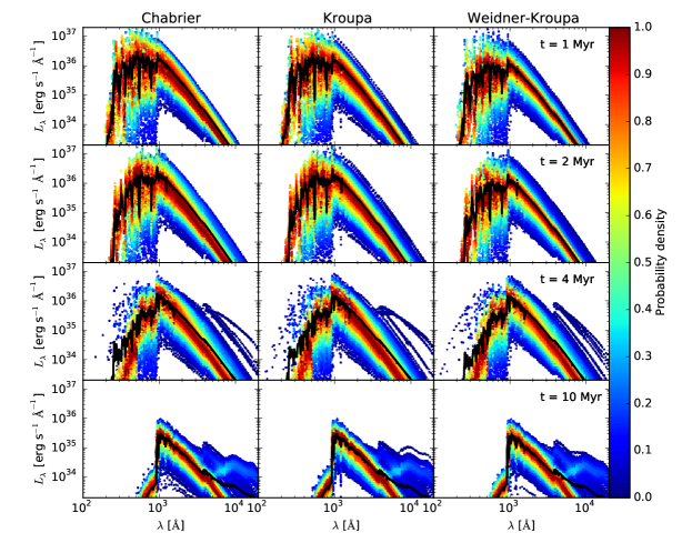
of 500 for three different IMFs. We create 1000 realizations each of such a population at times from Myr in intervals of 1 Myr, using the IMFs of Chabrier (2005), Kroupa (2002), and Weidner &
Kroupa (2006). The former two IMFs use STOP_NEAREST sampling, while the latter uses SORTED_SAMPLING, and is otherwise identical to the Kroupa (2002) IMF.
Figures 2 – 4 show the distributions of spectra and photometry that result from these simulations. Stochastic variations in photometry have been studied previously by a number of authors, going back to Chiosi et al. (1988), but to our knowledge no previous authors have investigated similar variations in spectra. The plots also demonstrate slug’s ability to evaluate the full probability distribution for both spectra and photometric filters, and reveal interesting phenomena that would not be accessible to a non-stochastic SPS code. In particular, Figure 2 shows that the mean specific luminosity can be orders of magnitude larger than the mode. The divergence is greatest at wavelengths of a few hundred Å at ages Myr, and wavelengths longer than Å at Myr. Indeed, at 4 Myr, it is noteworthy that the mean spectrum is actually outside the th percentile range. In this particular example, the range of wavelengths at 4 Myr where the mean spectrum is outside the th percentile corresponds to energies of Ryd. For a stellar population 4 Myr old, these photons are produced only by WR stars, and most prolifically by extremely hot WC stars. It turns out that a WC star is present of the time, but these cases are so much more luminous than when a WC star is not present that they are sufficient to drag the mean upward above the highest luminosities that occur in the of cases when no WC star is present.
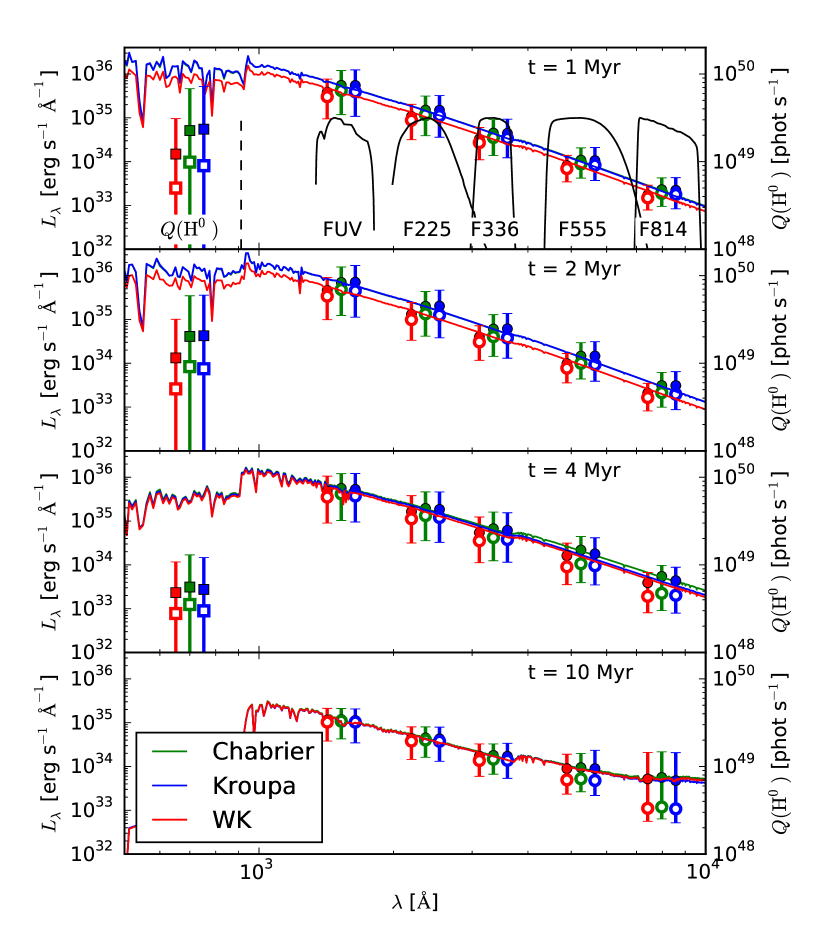
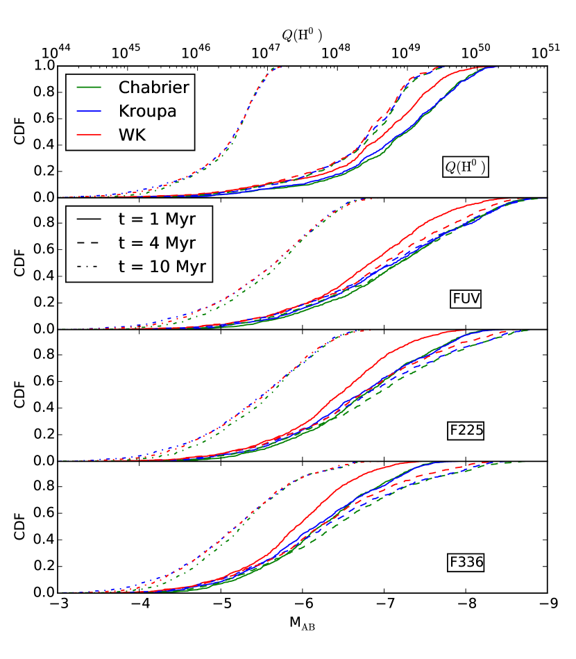
A similar phenomenon is visible in the photometry shown by Figure 3. In most of the filters the th percentile range is an order of magnitude wide, and for the ionizing luminosity and the HST UVIS F814W at 10 Myr the spread is more than two orders of magnitude, with significant offsets between mean and median indicating a highly asymmetric distribution. Figure 4, which shows the full distributions for several of the filters, confirms this impression: at early times the cumulative distribution functions are extremely broad, and the ionizing luminosity in particular shows a broad distribution at low and then a small number of simulations with large . Note that the percentile values are generally very well-determined by our set of 1000 simulations. Using the method described in Section 2.3.2 to compute the errors on the percentiles, we find that the 68% confidence interval on the 10th, 50th, and 90th percentile values is less than 0.1 dex wide at almost all times, filters, and IMFs. The only exception is at 1 Myr, where the 68% confidence interval on the 10th percentile of ionizing luminosity is dex wide.
The figures also illustrate slug’s ability to capture the “IGIMF effect” (Weidner & Kroupa, 2006) whereby sorted sampling produces a systematic bias toward lower luminosities at short wavelengths and early times. Both the spectra and photometric values for the Weidner & Kroupa (2006) IMF are systematically suppressed relative to the IMFs that use a sampling method that is less biased against high mass stars (cf. Figure 1).
3.3 Cluster Fraction and Cluster Mass Function
The first two examples have focused on simple stellar populations, namely collections of stars that are formed at coeval times to compose a “cluster” simulation. Our third example highlights slug’s ability to simulate composite stellar populations. Due to slug’s treatment of stellar clustering and stochasticity, simulations of such populations in slug differ substantially from those in non-stochastic SPS codes. Unlike in a conventional SPS code, the outcome of a slug simulation is sensitive to both the CMF and the fraction of stars formed in clusters. slug can therefore be applied to a wide variety of problems in which the fraction of stars formed within clusters or in the field becomes a critical parameter (e.g. Fumagalli et al., 2011).
The relevance of clusters in slug simulations arises from two channels. First, because stars form in clusters of finite size, and the interval between cluster formation events is not necessarily large compared to the lifetimes of individual massive stars, clustered star formation produces significantly more variability in the number of massive stars present at any given time than non-clustered star formation. We defer a discussion of this effect to the following section. Here, we instead focus on a second channel by which the CMF and influence the photometric output, which arises due to the method by which slug implements mass constraints. As discussed above, a realization of the IMF in a given cluster simulation is the result of the mass constraint imposed by the mass of the cluster, drawn from a CMF, and by the sampling technique chosen to approximate the target mass. Within “galaxy” simulations, a second mass constraint is imposed on the simulations as the SFH provides an implicit target mass for the galaxy, which in practice constrains each realization of the CMF. As a consequence, all the previous discussion on how the choice of stopping criterion affect the slug outputs in cluster simulations applies also to the way with which slug approximates the galaxy mass by drawing from the CMF. Through the parameter, the user has control on which level of this hierarchy contributes to the final simulation. In the limit of , slug removes the intermediate cluster container from the simulations: a galaxy mass is approximated by stars drawn from the IMF, without the constraints imposed by the CMF. Conversely, in the limit of , the input SFH constrains the shape of each realization of the CMF, which in turn shapes the mass spectrum of stars within the final outputs. As already noted in Fumagalli et al. (2011), this combined effect resembles in spirit the concept behind the IGIMF theory. However, the slug implementation is fundamentally different from the IGIMF, as our code does not require any a priori modification of the functional form of the input IMF and CMF, and each realization of these PDFs is only a result of random sampling of invariant PDFs.
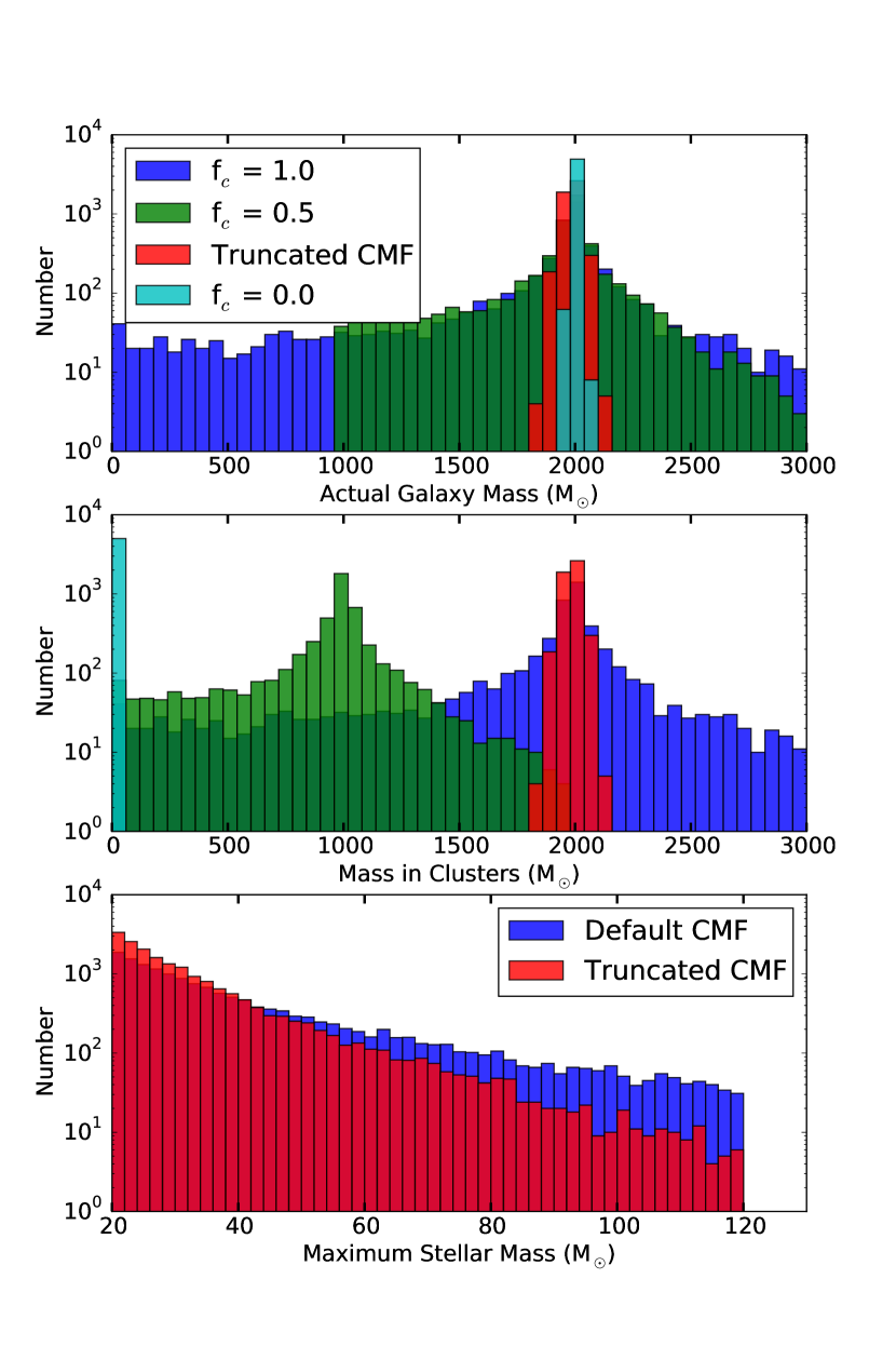
To offer an example that better illustrates these concepts, we perform four “galaxy” simulations with 5000 realizations. This number ensures that simulations are present in each mass bin considered in our analysis, thus providing a well converged distribution. Each simulation follows a single timestep of yr and assumes a Chabrier (2005) IMF, the default STOP_NEAREST condition, and an input SFR of 0.001 . Three of the four simulations further assume a default CMF of the form between M⊙, but three different choices of CMF (, 0.5, and 0.0). The fourth simulation still assumes and a CMF, but within the mass interval M⊙ (hereafter the truncated CMF). Results from these simulations are shown in Figure 5.
By imposing an input SFR of 0.001 for a time yr, we are in essence requesting that slug populates galaxies with M⊙ worth of stars. However, similarly to the case of cluster simulations, slug does not recover the input galaxy mass exactly, but it finds the best approximation based on the chosen stop criteria, the input CMF, and the choice of . This can be seen in the top panel of Figure 5, where we show the histograms of actual masses from the four simulations under consideration. For , slug is approximating the target galaxy mass simply by drawing stars from the IMF. As the typical stellar mass is much less than the desired galaxy mass, the mass constraint is not particularly relevant in these simulations and slug reproduces the target galaxy mass quite well, as one can see from the narrow distribution centered around M⊙. When , however, slug tries to approximate the target mass by means of much bigger building blocks, the clusters, thus increasing the spread of the actual mass distributions as seen for instance in the case. For , clusters as massive as M⊙ are potentially accessible during draws and, as a consequence of the STOP_NEAREST condition, one can notice a wide mass distribution together with a non-negligible tail at very low (including zero) actual galaxy masses. Including a M⊙ cluster to approximate a M⊙ galaxy would in fact constitute a larger error than leaving the galaxy empty! The importance of this effect obviously depends on how massive is the galaxy compared to the upper limit of the CMF. In our example, the choice of an unphysically small “galaxy” with is indeed meant to exacerbate the relevance of this mass constraint. By inspecting Figure 5, it is also evident that the resulting galaxy mass distributions are asymmetric, with a longer tail to lower masses. This is due to the fact that slug favours small building blocks over massive ones when drawing from a power-law CMF. This means that a draw of a cluster with mass comparable to the galaxy mass will likely occur after a few lower mass clusters have been included in the stellar population. Therefore, massive clusters are more likely to be excluded that retained in a simulation. For this reason, the galaxy target mass represents a limit inferior for the mean actual mass in each distribution.
The middle panel of Figure 5 shows the total amount of mass formed in clusters after one timestep. As expected, the fraction of mass in clusters versus field stars scales proportionally to , retaining the similar degree of dispersion noted for the total galaxy mass. Finally, by comparing the results of the simulations with the default CMF and the truncated CMF in all the three panels of Figure 5, one can appreciate the subtle difference that the choice of and CMF have on the output. Even in the case of , the truncated CMF still recovers the desired galaxy mass with high-precision. Obviously, this is an effect of the extreme choice made for the cluster mass interval, here between M⊙. In this case, for the purpose of constrained sampling, the CMF becomes indistinguishable from the IMF, and the simulations of truncated CMF and both recover the target galaxy mass with high accuracy. However, the simulations with truncated CMF still impose a constraint on the IMF, as shown in the bottom panel. In the case of truncated CMF, only clusters up to 100 M⊙ stars are formed, thus reducing the probability of drawing stars as massive as 120 M⊙ from the IMF.
This example highlights how the parameter and the CMF need to be chosen with care based on the problem that one wishes to simulate, as they regulate in a non-trivial way the scatter and the shape of the photometry distributions recovered by slug. In passing, we also note that slug’s ability to handle very general forms for the CMF and IMF makes our code suitable to explore a wide range of models in which the galaxy SFR, CMF and IMF depend on each other (e.g. as in the IGIMF; Weidner & Kroupa, 2006; Weidner et al., 2010).
3.4 Realizations of a Given Star Formation History
The study of SFHs in stochastic regimes is receiving much attention in the recent literature, both in the nearby and high-redshift universe (e.g. Kelson, 2014; Domínguez Sánchez et al., 2014; Boquien et al., 2014). As it can can handle arbitrary SFH in input, slug is suitable for the analysis of stochastic effects on galaxy SFR.
In previous papers, and particularly in da Silva et al. (2012) and da Silva et al. (2014), we have highlighted the conceptual difference between the input SFH and the outputs that are recovered from slug simulations. The reason for such a difference should now be clear from the above discussion: slug approximates an input SFH by means of discrete units, either in the form of clusters (for ), stars (for ), or a combination of both (for ). Thus, any smooth input function for the SFH (including a constant SFR) is approximated by slug as a series of bursts, that can described conceptually as the individual draws from the IMF or CMF. The effective SFH that slug creates in output is therefore an irregular function, which is the result of a superimposition of these multiple bursts. A critical ingredient is the typical time delays with which these bursts are combined, a quantity that is implicitly set by the SFH evaluated in each timestep and by the typical mass of the building blocks used to assemble the simulated galaxies.
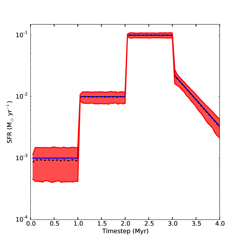
A simple example, which also highlights slug’s flexibility in handling arbitrary SFHs in input, is presented in Figure 6. For this calculation, we run 5000 slug models with default parameters and . The input SFH is defined by three segments of constant SFR across three time intervals of 1 Myr each, plus a fourth segment of exponentially decaying SFR with timescale 0.5 Myr. Figure 6 shows how the desired SFH is recovered by slug on average, but individual models show a substantial scatter about the mean, especially at low SFRs. An extensive discussion of this result is provided in section 3.2 of da Silva et al. (2012).
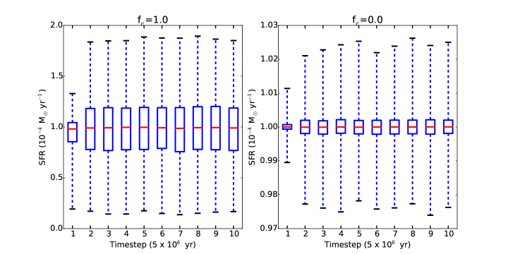
Briefly, at the limit of many bursts and small time delays (i.e. for high SFRs and/or when slug populates galaxies mostly with stars for ), the output SFHs are reasonable approximations of the input SFH. Conversely, for small sets of bursts and for long time delays (i.e. for low SFRs and/or when slug populates galaxies mostly with massive clusters for ), the output SFHs are only a coarse representation of the desired input SFH. This behaviour is further illustrated by Figure 7, in which we show the statistics of the SFHs of 5000 galaxy simulations. These simulations are performed assuming a constant SFR and two choices of fraction of stars formed in clusters, and 0. One can notice that, in both cases, a “flickering” SFH is recovered, but that a much greater scatter is evident for the case when clusters are used to assemble the simulated galaxies.
From this discussion, it clearly emerges that each slug simulation will have an intrinsically bursty SFH, regardless to the user-set input, as already pointed out in Fumagalli et al. (2011) and da Silva et al. (2012). It is noteworthy that this fundamental characteristic associated to the discreteness with which star formation occurs in galaxies has also been highlighted by recent analytic and simulation work (e.g. Kelson, 2014; Domínguez Sánchez et al., 2014; Boquien et al., 2014; Rodríguez Espinosa et al., 2014). This effect, and the consequences it has on many aspects of galaxy studies including the completeness of surveys or the use of SFR indicators, is receiving great attention particularly in the context of studies at high redshift. Slug thus provides a valuable tool for further investigation into this problem, particularly because our code naturally recovers a level of burstiness imposed by random sampling, which does not need to be specified a-priori as in some of the previous studies.
3.5 Cluster Disruption
When performing galaxy simulations, cluster disruption can be enabled in slug. In this new release of the code, slug handles cluster disruption quite flexibly, as the user can now specify the cluster lifetime function (CLF), which is a PDF from which the lifetime of each cluster is drawn. This implementation generalises the original cluster disruption method described in da Silva et al. (2012) to handle the wide range of lifetimes observed in nearby galaxies (A. Adamo et al., 2015, submitted). We note however that the slug default CLF still follows a power law of index between 1 Myr and 1 Gyr as in Fall et al. (2009).
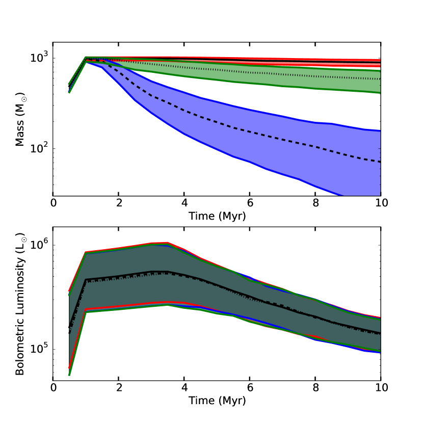
To demonstrate the cluster disruption mechanism, we run three simulations of 1000 trials each. These simulations follow the evolution of a burst of 1000 M⊙ between Myr with a timestep of yr up to a maximum time of 10 Myr. All stars are formed in clusters. The three simulations differ only for the choice of cluster disruption: one calculation does not implement any disruption law, while the other two assume a CLF in the form of a power law with indices and between Myr. Results from these calculations are shown in Figure 8.
The total mass in clusters, as expected, rises till a maximum of 1000 M⊙ at 1 Myr, at which point it remains constant for the non-disruption case, while it declines according to the input power law in the other two simulations. When examining the galaxy bolometric luminosity, one can see that the cluster disruption as no effect on the galaxy photometry. In this example, all stars are formed in clusters and thus all the previous discussion on the mass constraint also applies here. However, after formation, clusters and galaxies are passively evolved in slug by computing the photometric properties as a function of time. When a cluster is disrupted, slug stops tagging it as a “cluster” object, but it still follows the contribution that these stars make to the integrated “galaxy” properties. Clearly, more complex examples in which star formation proceeds both in the field and in clusters following an input SFH while cluster disruption is enabled would exhibit photometric properties that are set by the passive evolution of previously-formed stars and by the zero-age main sequence properties of the newly formed stellar populations, each with its own mass constraint.
3.6 Dust Extinction and Nebular Emission
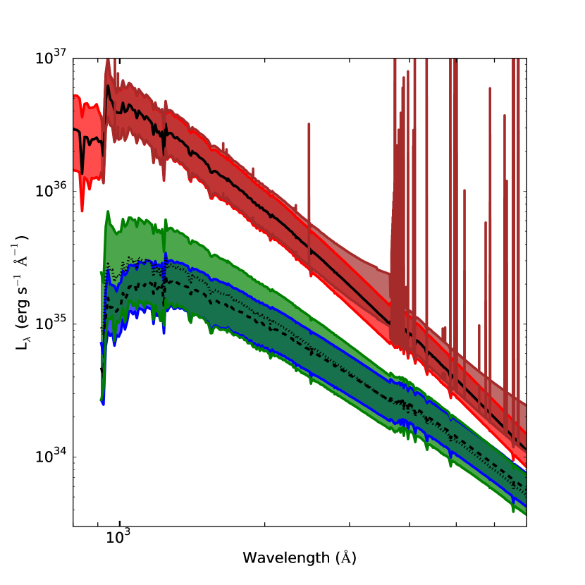
In this section we offer an example of simulations which implement dust extinction and nebular emission in post-processing, two new features offered starting from this release of the code (see Section 2.1.2). Figure 9 shows the stellar spectra of three slug simulations (in green, blue, and red respectively) of a galaxy that is forming stars with a SFR of M⊙ yr-1. During these simulations, each of 5000 trials, the cluster fraction is set to and photometry is evaluated at yr. Three choices of extinction law are adopted: the first simulation has no extinction, while the second and third calculations implement the Calzetti et al. (2000) extinction law. In one case, a deterministic uniform screen with mag is applied to the emergent spectrum, while in the other case the value of is drawn for each model from a lognormal distribution with mean 1.0 mag and dispersion of dex (the slug default choice).
As expected, the simulations with a deterministic uniform dust screen closely match the results of the non-dusty case, with a simple wavelength-dependent shift in logarithmic space. For the probabilistic dust model, on the other hand, the simulation results are qualitatively similar to the non-dusty case, but display a much greater scatter due to the varying degree of extinction that is applied in each trial. This probabilistic dust implementation allows one to more closely mimic the case of non-uniform dust extinction, in which different line of sights may be subject to a different degree of obscuration. One can also see how spectra with dust extinction are computed only for Å. This is not a physical effect, but it is a mere consequence of the wavelength range for which the extinction curves have been specified.
Finally, we also show in Figure 9 a fourth simulation (brown colour), which is computed including nebular emission with slug’s default parameters: and (see Appendix B). In this case, the cutoff visible at the ionisation edge is physical, as slug reprocesses the ionising radiation into lower frequency nebular emission according to the prescriptions described in Section 2.1.2. One can in fact notice, besides the evident contribution from recombination lines, an increased luminosity at Å that is a consequence of free-free, bound-free, and two-photon continuum emission.
3.7 Coupling cloudy to slug Simulations
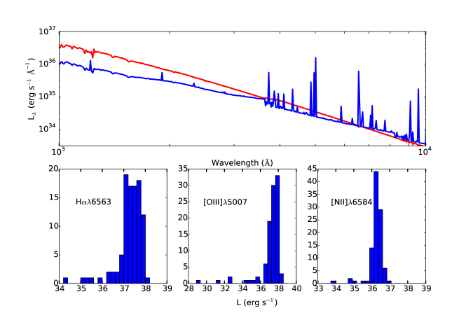
In this section, we demonstrate the capability of the cloudy_slug package that inputs the results of slug simulations into the cloudy radiative transfer code. For this, we run 100 realizations of a “galaxy” simulation following a single timestep of yr. The input parameters for the simulation are identical to those in Section 3.3. The galaxy is forming stars at a rate of 0.001 M⊙ yr-1 with . We then pipe the slug output into cloudy to simulate H ii regions in integrated mode, following the method discussed in Section 2.2. In these calculations, we assume the default parameters in cloudy_slug, and in particular a density in the surroundings of the H ii regions of .
Results are shown in Figure 10. In the top panel, the median of the 100 slug SEDs is compared to the median of the 100 SEDs returned by cloudy, which adds the contribution of both the transmitted and the diffuse radiation. As expected, the processed cloudy SEDs resemble the input slug spectra. Photons at short wavelengths are absorbed inside the H ii regions and are converted into UV, optical, and IR photons, which are then re-emitted within emission lines or in the continuum.666We do not show the region below 912 Å in Figure 10 so that we can zoom-in on the features in the optical region. The nebula-processed spectrum also shows the effects of dust absorption within the H ii region and its surrounding shell, which explains why the nebular spectrum is suppressed below the intrinsic stellar one at short wavelengths.
The bottom panel shows the full distribution of the line fluxes in three selected transitions: H, [O iii] and [N ii] . These distributions highlight how the wavelength-dependent scatter in the input slug SEDs is inherited by the reprocessed emission lines, which exhibit a varying degree of stochasticity. The long tail of the distribution at low H luminosity is not well-characterized by the number of simulations we have run, but this could be improved simply by running a larger set of simulations. We are in the process of completing a much more detailed study of stochasticity in line emission (T. Rendahl et al., in preparation).
3.8 Bayesian Inference of Star Formation Rates
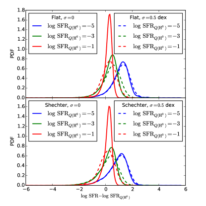
To demonstrate the capabilities of SFR_slug, we consider the simple example of using a measured ionizing photon flux to infer the true SFR. We use the library described above and in da Silva et al. (2014), and consider ionizing fluxes which correspond to , , and yr-1 using an estimate that neglects stochasticity and simply adopts the ionizing luminosity to SFR conversion appropriate for an infinitely-sampled IMF and SFH. We then use SFR_slug to compute the true posterior probability distribution on the SFR using these measurements; we do so on a grid of 128 points, using photometric errors of 0 and dex, and using two different prior probability distributions: one that is flat in (i.e., ), and one following the Schechter function distribution of SFRs reported by Bothwell et al. (2011), , where and yr-1.
Figure 11 shows the posterior PDFs we obtain, which we normalised to have unit integral. Consistent with the results reported by da Silva et al. (2014), at SFRs of yr-1, the main effect of stochasticity is to introduce a few tenths of a dex uncertainty into the SFR determination, while leaving the peak of the probability distribution centered close to the value predicted by the point mass estimate. For SFRs of or yr-1, the true posterior PDF is very broad, so that even with a dex uncertainty on the photometry, the uncertainty on the true SFR is dominated by stochastic effects. Moreover, the peak of the PDF differs from the value given by the point mass estimate by more than a dex, indicating a systematic bias. These conclusions are not new, but we note that the improved computational method described in Section 2.3 results in a significant code speedup compared to the method presented in da Silva et al. (2014). The time required for SFR_slug to compute the full posterior PDF for each combination of , photometric error, and prior probability distribution is seconds on a single core of a laptop (excluding the startup time to read the library). Thus this method can easily be used to generate posterior probability distributions for large numbers of measurement in times short enough for interactive use.
3.9 Bayesian Inference of Star Cluster Properties
To demonstrate the capabilities of cluster_slug, we re-analyse the catalog of star clusters in the central regions of M83 described by Chandar et al. (2010). These authors observed M83 with Wide Field Camera 3 aboard the Hubble Space Telescope, and obtained measurements for star clusters in the filters F336W, F438W, F555W, F814W, and F657N (H). They used these measurements to assign each cluster a mass and age by comparing the observed photometry to simple stellar population models using Bruzual & Charlot (2003) models for a twice-solar metallicity population, coupled with a Milky Way extinction law; see Chandar et al. (2010) for a full description of their method. This catalog has also been re-analyzed by Fouesneau et al. (2012) using their stochastic version of pegagse. Their method, which is based on minimization over a large library of simulated clusters, is somewhat different than our kernel density-based one, but should share a number of similarities – see Fouesneau & Lançon (2010) for more details on their method. We can therefore compare our results to theirs as well.
We downloaded Chandar et al.’s “automatic” catalog from MAST777https://archive.stsci.edu/ and used cluster_slug to compute posterior probability distributions for the mass and age of every cluster for which photometric values were available in all five filters. We used the photometric errors included in the catalog in this analysis, coupled to the default choice of bandwidth in cluster_slug, and a prior probability distribution that is flat in the logarithm of the age and , while varying with mass as . We used our library computed for the Padova tracks and a Milky Way extinction curve, including nebular emission. The total time required for cluster_slug to compute the marginal probability distributions of mass and age on grids of 128 logarithmically-spaced points each was seconds per marginal PDF ( seconds for 2 PDFs each on the entire catalog of 656 clusters), using a single CPU. The computation can be parallelized trivially simply by running multiple instances of cluster_slug on different parts of the input catalog.
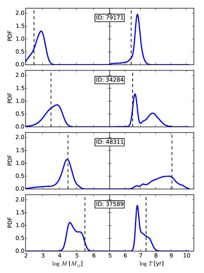
In Figure 12 we show example posterior probabilities distributions for cluster mass and age as returned by cluster_slug, and in Figure 13 we show the median and interquartile ranges for cluster mass and age computed from cluster_slug compared to those determined by Chandar et al. (2010)888The mass and age estimates plotted are from the most up-to-date catalog maintained by R. Chandar (2015, priv. comm.).. The points in Figure 13 are color-coded by the “photometric distance” between the observed photometric values and the 5th closest matching model in the cluster_slug library, where the photometric distance is defined as
| (29) |
where and are the observed magnitude and the magnitude of the cluster_slug simulation in filter , and the sum is over all 5 filters used in the analysis.
We can draw a few conclusions from these plots. Examining Figure 12, we see that cluster_slug in some cases identifies a single most likely mass or age with a fairly sharp peak, but in other cases identifies multiple distinct possible fits, so that the posterior PDF is bimodal. In these cases the best fit identified by Chandar et al. usually matches one of the peaks found by cluster_slug. The ability to recover bimodal posterior PDFs represents a distinct advantage of cluster_slug’s method, since it directly indicates cases where there is a degeneracy in possible models.
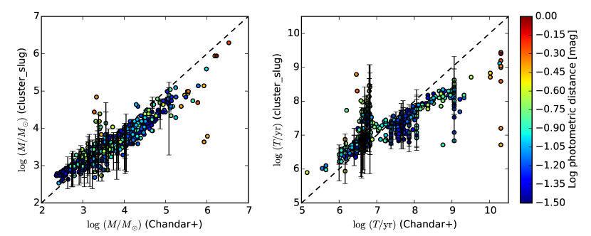
From Figure 13, we see that, with the exception of a few catastrophic outliers, the median masses returned by cluster_slug are comparable to those found by Chandar et al. The ages show general agreement, but less so than the masses. For the ages, disagreements come in two forms. First, there is a systematic difference that cluster_slug tends to assign younger ages for any cluster for which Chandar et al. have assigned an age yr. For many of these clusters the line is still within the 10th - 90th percentile range, but the 50th percentile is well below the line. The second type of disagreement is more catastrophic. We find that there are are a fair number of clusters for which Chandar et al. assign ages of Myr, while cluster_slug produces ages dex larger. Conversely, for the oldest clusters in Chandar et al.’s catalog, cluster_slug tends to assign significantly younger ages.
The differences in ages probably have a number of causes. The fact that our 50th percentile ages tend to be lower than those derived by Chandar et al. (2010) even when the disagreement is not catastrophic is likely a result of the broadness of the posterior PDFs, and the fact that we are exploring the full posterior PDF rather than selecting a single best fit. For example, in the middle two panels of Figure 12, the peak of the posterior PDF is indeed close to the value assigned by Chandar et al. However, the PDF is also very broad, so that the 50th percentile can be displaced very significantly from the peak. We note that this also likely explains why our Figure 13 appears to indicate greater disagreement between stochastic and non-stochastic models than do Fouesneau et al. (2012)’s Figures 18 and 20, which ostensibly make the same comparison. Fouesneau et al. identify the peak in the posterior PDF, but do not explore its full shape. When the PDF is broad or double-peaked, this can be misleading.
The catastrophic outliers are different in nature, and can be broken into two categories. The disagreement at the very oldest ages assigned by Chandar et al. (2010) is easy to understand: the very oldest clusters in M83 are globular clusters with substantially sub-Solar metallicities, while our library is for Solar metallicity. Thus our library simply does not contain good matches to the colors of these clusters, as is apparent from their large photometric distances (see more below). The population of clusters for which Chandar et al. (2010) assign Myr ages, while the stochastic models assign much older ages, is more interesting. Fouesneau et al. (2012) found a similar effect in their analysis, and their explanation of the phenomenon holds for our models as well. These clusters have relatively red colors and lack strong H emission, properties that can be matched almost equally well either by a model at an age of Myr (old enough for ionization to have disappeared) with relatively low mass and high extinction, or by a model at a substantially older age with lower extinction and higher total mass. This is a true degeneracy, and the stochastic and non-stochastic models tend to break the degeneracy in different directions. The ages assigned to these clusters also tend to be quite dependent on the choice of priors (Krumholz et al., 2015, in preparation).
We can also see from Figure 13 that, for the most part and without any fine-tuning, the default cluster_slug library does a very good job of matching the observations. As indicated by the color-coding, for most of the observed clusters, the cluster_slug library contains at least 5 simulations that match the observations to a photometric distance of a few tenths of a magnitude. Quantitatively, 90% of the observed clusters have a match in the library that is within 0.15 mag, and 95% have a match within 0.20 mag; for 5th nearest neighbors, these figures rise to 0.18 and 0.22 mag. There are, however, some exceptions, and these are clusters for which the cluster_slug fit differs most dramatically from the Chandar et al. one. The worst agreement is found for the clusters for which Chandar et al. (2010) assigns the oldest ages, and, as noted above, this is almost certainly a metallicity effect. However, even eliminating these cases there are clusters for which the closest match in the cluster_slug library is at a photometric distance of mag. It is possible that these clusters have extinctions and thus outside the range covered by the library, that these are clusters where our failure to make the appropriate aperture corrections makes a large difference, or that the disagreement has some other cause. These few exceptions notwithstanding, this experiment makes it clear that, for the vast majority of real star cluster observations, cluster_slug can return a full posterior PDF that properly accounts for stochasticity and other sources of error such as age-mass degeneracies, and can do so at an extremely modest computational cost.
4 Summary and Prospects
As telescopes gains in power, observations are able to push to ever smaller spatial and mass scales. Such small scales are often the most interesting, since they allow us to observe fine details of the process by which gas in galaxies is transformed into stars. However, taking advantage of these observational gains will require the development of a new generation of analysis tools that dispense with the simplifying assumptions that were acceptable for processing lower-resolution data. The goal of this paper is to provide such a next-generation analysis tool that will allow us to extend stellar population synthesis methods beyond the regime where stellar initial mass functions (IMFs) and star formation histories (SFHs) are well-sampled. The slug code we describe here makes it possible to perform full SPS calculations with nearly-arbitrary IMFs and SFHs in the realm where neither distribution is well-sampled; the accompanying suite of software tools makes it possible to use libraries of slug simulations to solve the inverse problem of converting observed photometry to physical properties of stellar populations outside the well-sampled regime. In addition to providing a general software framework for this task, bayesphot, we provide software to solve the particular problems of inferring the posterior probability distribution for galaxy star formation rates (SFR_slug) and star cluster masses, ages, and extinctions (cluster_slug) from unresolved photometry.
In upcoming work, we will use slug and its capability to couple to cloudy (Ferland et al., 2013) to evaluate the effects of stochasticity on emission line diagnostics such as the BPT diagram (Baldwin et al., 1981), and to analyze the properties of star clusters in the new Legacy Extragalactic UV Survey (Calzetti et al., 2015). However, we emphasize that slug, its companion tools, and the pre-computed libraries of simulations we have created are open source software, and are available for community use on these and other problems.
Acknowledgements
The authors thank Michelle Myers for assistance, and Aida Wofford, Angela Adamo, and Janice Lee for comments on the manuscript. MRK acknowledges support from Hubble Space Telescope programs HST-AR-13256 and HST-GO-13364, provided by NASA through a grant from the Space Telescope Science Institute, which is operated by the Association of Universities for Research in Astronomy, Inc., under NASA contract NAS 5-26555. MF acknowledges support by the Science and Technology Facilities Council, grant number ST/L00075X/1. Some of the data presented in this paper were obtained from the Mikulski Archive for Space Telescopes (MAST). STScI is operated by the Association of Universities for Research in Astronomy, Inc., under NASA contract NAS5-26555. Support for MAST for non-HST data is provided by the NASA Office of Space Science via grant NNX13AC07G and by other grants and contracts. This work used the UCSC supercomputer Hyades, which is supported by the NSF (award number AST-1229745), and the DiRAC Data Centric system at Durham University, operated by the Institute for Computational Cosmology on behalf of the STFC DiRAC HPC Facility (www.dirac.ac.uk). This equipment was funded by BIS National E-infrastructure capital grant ST/K00042X/1, STFC capital grant ST/H008519/1, and STFC DiRAC Operations grant ST/K003267/1 and Durham University. DiRAC is part of the National E-Infrastructure.
References
- Akima (1970) Akima H., 1970, J. Assoc. Comput. Mach., 17, 589
- Anders et al. (2013) Anders P., Kotulla R., de Grijs R., Wicker J., 2013, ApJ, 778, 138
- Andrews et al. (2013) Andrews J. E., et al., 2013, ApJ, 767, 51
- Andrews et al. (2014) Andrews J. E., et al., 2014, ApJ, 793, 4
- Asa’d & Hanson (2012) Asa’d R. S., Hanson M. M., 2012, MNRAS, 419, 2116
- Astropy Collaboration et al. (2013) Astropy Collaboration et al., 2013, A&A, 558, A33
- Baldwin et al. (1981) Baldwin J. A., Phillips M. M., Terlevich R., 1981, Proc. Astron. Soc. Pac., 93, 5
- Boquien et al. (2014) Boquien M., Buat V., Perret V., 2014, A&A, 571, A72
- Bothwell et al. (2011) Bothwell M. S., et al., 2011, MNRAS, 415, 1815
- Bouchet et al. (1985) Bouchet P., Lequeux J., Maurice E., Prevot L., Prevot-Burnichon M. L., 1985, A&A, 149, 330
- Bruzual & Charlot (2003) Bruzual G., Charlot S., 2003, MNRAS, 344, 1000
- Calzetti et al. (2000) Calzetti D., Armus L., Bohlin R. C., Kinney A. L., Koornneef J., Storchi-Bergmann T., 2000, ApJ, 533, 682
- Calzetti et al. (2015) Calzetti D., et al., 2015, AJ, 149, 51
- Cerviño (2013) Cerviño M., 2013, New Astron. Rev., 57, 123
- Cerviño & Luridiana (2004) Cerviño M., Luridiana V., 2004, A&A, 413, 145
- Cerviño & Luridiana (2006) Cerviño M., Luridiana V., 2006, A&A, 451, 475
- Cerviño & Valls-Gabaud (2003) Cerviño M., Valls-Gabaud D., 2003, MNRAS, 338, 481
- Cerviño et al. (2013) Cerviño M., Román-Zúñiga C., Luridiana V., Bayo A., Sánchez N., Pérez E., 2013, A&A, 553, A31
- Cervino & Luridiana (2005) Cervino M., Luridiana V., 2005, ArXiv Astrophysics e-prints,
- Chabrier (2003) Chabrier G., 2003, Proc. Astron. Soc. Pac., 115, 763
- Chabrier (2005) Chabrier G., 2005, in Corbelli E., Palla F., Zinnecker H., eds, Astrophysics and Space Science Library Vol. 327, The Initial Mass Function 50 Years Later. Springer, Dordrecht, pp 41–+
- Chandar et al. (2010) Chandar R., et al., 2010, ApJ, 719, 966
- Charlot & Bruzual (1991) Charlot S., Bruzual A. G., 1991, ApJ, 367, 126
- Chiosi et al. (1988) Chiosi C., Bertelli G., Bressan A., 1988, A&A, 196, 84
- Conroy & Gunn (2010) Conroy C., Gunn J. E., 2010, ApJ, 712, 833
- Conroy et al. (2009) Conroy C., Gunn J. E., White M., 2009, ApJ, 699, 486
- Conroy et al. (2010) Conroy C., White M., Gunn J. E., 2010, ApJ, 708, 58
- Cook et al. (2012) Cook D. O., et al., 2012, ApJ, 751, 100
- Dalcanton et al. (2012) Dalcanton J. J., et al., 2012, ApJS, 200, 18
- Domínguez Sánchez et al. (2014) Domínguez Sánchez H., et al., 2014, MNRAS, 441, 2
- Dopita et al. (2002) Dopita M. A., Groves B. A., Sutherland R. S., Binette L., Cecil G., 2002, ApJ, 572, 753
- Draine (2011) Draine B. T., 2011, Physics of the Interstellar and Intergalactic Medium. Princeton University Press: Princeton, NJ
- Ekström et al. (2012) Ekström S., et al., 2012, A&A, 537, A146
- Ercolano & Storey (2006) Ercolano B., Storey P. J., 2006, MNRAS, 372, 1875
- Fall et al. (2009) Fall S. M., Chandar R., Whitmore B. C., 2009, ApJ, 704, 453
- Ferland et al. (2013) Ferland G. J., et al., 2013, Rev. Mex. Astron. Astrop., 49, 137
- Fioc & Rocca-Volmerange (1997) Fioc M., Rocca-Volmerange B., 1997, A&A, 326, 950
- Fitzpatrick (1999) Fitzpatrick E. L., 1999, Proc. Astron. Soc. Pac., 111, 63
- Foreman-Mackey et al. (2013) Foreman-Mackey D., Hogg D. W., Lang D., Goodman J., 2013, Proc. Astron. Soc. Pac., 125, 306
- Forero-Romero & Dijkstra (2013) Forero-Romero J. E., Dijkstra M., 2013, MNRAS, 428, 2163
- Fouesneau & Lançon (2010) Fouesneau M., Lançon A., 2010, A&A, 521, A22
- Fouesneau et al. (2012) Fouesneau M., Lançon A., Chandar R., Whitmore B. C., 2012, ApJ, 750, 60
- Fouesneau et al. (2014) Fouesneau M., et al., 2014, ApJ, 786, 117
- Fumagalli et al. (2011) Fumagalli M., da Silva R. L., Krumholz M. R., 2011, ApJ, 741, L26
- Georgy et al. (2013) Georgy C., et al., 2013, A&A, 558, A103
- Girardi et al. (2000) Girardi L., Bressan A., Bertelli G., Chiosi C., 2000, A&AS, 141, 371
- Haas & Anders (2010) Haas M. R., Anders P., 2010, A&A, 512, A79
- Hillier & Miller (1998) Hillier D. J., Miller D. L., 1998, ApJ, 496, 407
- Jones et al. (2013a) Jones T., Ellis R. S., Richard J., Jullo E., 2013a, ApJ, 765, 48
- Jones et al. (2013b) Jones T. A., Ellis R. S., Schenker M. A., Stark D. P., 2013b, ApJ, 779, 52
- Kelson (2014) Kelson D. D., 2014, ApJ,
- Köppen et al. (2007) Köppen J., Weidner C., Kroupa P., 2007, MNRAS, 375, 673
- Kroupa (2002) Kroupa P., 2002, Science, 295, 82
- Krumholz (2014) Krumholz M. R., 2014, Physics Reports, 539, 49
- Krumholz & Matzner (2009) Krumholz M. R., Matzner C. D., 2009, ApJ, 703, 1352
- Krumholz et al. (2009) Krumholz M. R., McKee C. F., Tumlinson J., 2009, ApJ, 693, 216
- Lada & Lada (2003) Lada C. J., Lada E. A., 2003, ARA&A, 41, 57
- Landini et al. (1984) Landini M., Natta A., Salinari P., Oliva E., Moorwood A. F. M., 1984, A&A, 134, 284
- Leitherer et al. (1999) Leitherer C., et al., 1999, ApJS, 123, 3
- Leitherer et al. (2010) Leitherer C., Ortiz Otálvaro P. A., Bresolin F., Kudritzki R.-P., Lo Faro B., Pauldrach A. W. A., Pettini M., Rix S. A., 2010, ApJS, 189, 309
- Leitherer et al. (2014) Leitherer C., Ekström S., Meynet G., Schaerer D., Agienko K. B., Levesque E. M., 2014, ApJS, 212, 14
- Lejeune et al. (1997) Lejeune T., Cuisinier F., Buser R., 1997, A&AS, 125, 229
- Leroy et al. (2013) Leroy A. K., et al., 2013, AJ, 146, 19
- Maíz Apellániz (2009) Maíz Apellániz J., 2009, ApJ, 699, 1938
- McKee & Williams (1997) McKee C. F., Williams J. P., 1997, ApJ, 476, 144
- Meynet et al. (1994) Meynet G., Maeder A., Schaller G., Schaerer D., Charbonnel C., 1994, A&AS, 103, 97
- Murray & Rahman (2010) Murray N., Rahman M., 2010, ApJ, 709, 424
- Nussbaumer & Schmutz (1984) Nussbaumer H., Schmutz W., 1984, A&A, 138, 495
- Osterbrock (1989) Osterbrock D. E., 1989, Astrophysics of gaseous nebulae and active galactic nuclei. University Science Books
- Pauldrach et al. (2001) Pauldrach A. W. A., Hoffmann T. L., Lennon M., 2001, A&A, 375, 161
- Pflamm-Altenburg et al. (2007) Pflamm-Altenburg J., Weidner C., Kroupa P., 2007, ApJ, 671, 1550
- Popescu & Hanson (2009) Popescu B., Hanson M. M., 2009, AJ, 138, 1724
- Popescu & Hanson (2010a) Popescu B., Hanson M. M., 2010a, ApJ, 713, L21
- Popescu & Hanson (2010b) Popescu B., Hanson M. M., 2010b, ApJ, 724, 296
- Popescu & Hanson (2014) Popescu B., Hanson M. M., 2014, ApJ, 780, 27
- Popescu et al. (2012) Popescu B., Hanson M. M., Elmegreen B. G., 2012, ApJ, 751, 122
- Rodríguez Espinosa et al. (2014) Rodríguez Espinosa J. M., et al., 2014, MNRAS, 444, L68
- Salpeter (1955) Salpeter E. E., 1955, ApJ, 121, 161
- Schaller et al. (1992) Schaller G., Schaerer D., Meynet G., Maeder A., 1992, A&AS, 96, 269
- da Silva et al. (2012) da Silva R. L., Fumagalli M., Krumholz M., 2012, ApJ, 745, 145
- da Silva et al. (2014) da Silva R. L., Fumagalli M., Krumholz M. R., 2014, MNRAS, 444, 3275
- Smith et al. (2002) Smith L. J., Norris R. P. F., Crowther P. A., 2002, MNRAS, 337, 1309
- Storey & Hummer (1995) Storey P. J., Hummer D. G., 1995, MNRAS, 272, 41
- Vassiliadis & Wood (1993) Vassiliadis E., Wood P. R., 1993, ApJ, 413, 641
- Vázquez & Leitherer (2005) Vázquez G. A., Leitherer C., 2005, ApJ, 621, 695
- Verdolini et al. (2013) Verdolini S., Yeh S. C. C., Krumholz M. R., Matzner C. D., Tielens A. G. G. M., 2013, ApJ, 769, 12
- Weidner & Kroupa (2006) Weidner C., Kroupa P., 2006, MNRAS, 365, 1333
- Weidner et al. (2004) Weidner C., Kroupa P., Larsen S. S., 2004, MNRAS, 350, 1503
- Weidner et al. (2010) Weidner C., Kroupa P., Bonnell I. A. D., 2010, MNRAS, 401, 275
- Weidner et al. (2014) Weidner C., Kroupa P., Pflamm-Altenburg J., 2014, MNRAS, 441, 3348
- Yeh & Matzner (2012) Yeh S. C. C., Matzner C. D., 2012, ApJ, 757, 108
- Yeh et al. (2013) Yeh S. C. C., Verdolini S., Krumholz M. R., Matzner C. D., Tielens A. G. G. M., 2013, ApJ, 769, 11
- de Meulenaer et al. (2013) de Meulenaer P., Narbutis D., Mineikis T., Vansevičius V., 2013, A&A, 550, A20
- de Meulenaer et al. (2014) de Meulenaer P., Narbutis D., Mineikis T., Vansevičius V., 2014, A&A, 569, A4
- de Meulenaer et al. (2015) de Meulenaer P., Narbutis D., Mineikis T., Vansevičius V., 2015, A&A, 574, A66
Appendix A Implementation Details and Capabilities
Here we describe some details of slug’s current implementation. These capabilities may be expanded in future versions, but we include this description here both to demonstrate the code’s flexibility, and to discuss some subtleties that may be of use to those interested in implementing similar codes.
A.1 Probability Distribution Functions
Slug uses a large number of probability distribution functions (PDFs). In particular, the IMF, the cluster mass function (CMF), and the the star formation history (SFH) are all required to be PDFs, and the extinction, output time, and (for simulations of simple stellar populations) can optionally be described by PDFs as well. In slug, PDFs, can be specified as a sum of an arbitrary number of piecewise continuous segments,
| (30) |
where the normalizations for each segment are free parameters, as are the parameters and that denote the lower and upper limits for each segment (i.e., the function is non-zero only in the range ). The functions can take any of the functional forms listed in Table 2, and the software is modular so that additional functional forms can be added very easily. In the most common cases, the segment limits and normalizations will be chosen so that the segments are contiguous with one another and the overall PDF continuous, i.e., and . However, this is not a required condition, and the limits, normalizations, and number of segments can be varied arbitrarily. In particular, segments are allowed to overlap or to be discontinuous (as they must in the case of function segments); thus for example one could treat the star formation history of a galaxy as a sum of two components, one describing the bulge and one describing the disc. Slug ships with the following IMFs pre-defined for user convenience: Salpeter (1955), Kroupa (2002), Chabrier (2003), and Chabrier (2005).
| Name | Functional form, | Parameters999In addition to the segment-specific parameters listed, all segments also allow the upper and lower cutoffs and as free parameters. |
|---|---|---|
| delta | 101010For delta segments, we require that . | |
| exponential | ||
| lognormal | , | |
| normal | , | |
| powerlaw | ||
| schechter | , |
When drawing a finite total mass, in addition to the mass distribution, one must also specify a sampling method to handle the fact that one will not be able to hit the target mass perfectly when drawing discrete objects. Slug allows users to choose a wide range of methods for this purpose, which we describe briefly here following the naming convention used in the code. The majority of these methods are described in Haas & Anders (2010).
-
•
STOP_NEAREST: draw from the IMF until the total mass of the population exceeds . Either keep or exclude the final star drawn depending on which choice brings the total mass closer to the target value. Unless a different scheme is deemed necessary, this is the preferred and default choice of slug, as this sampling technique ensures that the stochastic solution converges towards the deterministic one at the limit of sufficiently large .
-
•
STOP_BEFORE: same as STOP_NEAREST, but the final star drawn is always excluded.
-
•
STOP_AFTER: same as STOP_NEAREST, but the final star drawn is always kept.
-
•
STOP_50: same as STOP_NEAREST, but keep or exclude the final star with 50% probability regardless of which choice gets closer to the target.
-
•
NUMBER: draw exactly objects, where is the expectation value for the mass of an object produced by a single draw, and the value of is rounded to the nearest integer. Note that this method can be used to handle the case of characterizing a population as containing a particular number of objects as opposed to a particular total mass, simply by choosing .
-
•
POISSON: draw exactly objects, where the value of is chosen from a Poisson distribution with expectation value
-
•
SORTED_SAMPLING111111This method replaces the IGIMF method implemented in the earlier version of slug (da Silva et al., 2012), which was based on the Weidner et al. (2010) version of the integrated galactic IMF (IGIMF) model. In Weidner et al. (2010)’s formulation, the upper cutoff of the IMF in a star cluster depends explicitly (rather than simply due to size-of-sample effects) on the total mass of the cluster. This model has been fairly comprehensively excluded by observations since the original slug code was developed (Fumagalli et al., 2011; Andrews et al., 2013, 2014), and Weidner et al. (2014) advocated dropping that formulation of the IGIMF in favor of the earlier Weidner & Kroupa (2006) one. See Krumholz (2014) for a recent review discussing the issue.: this method was introduced by Weidner & Kroupa (2006). In it, one first draws exactly objects as in the NUMBER method. If the resulting total mass is less than , the procedure is repeated recursively using a target mass until . Finally, one sorts the resulting list of objects from least to most massive, and then keeps or removes the final, most massive using a STOP_NEAREST policy.
Finally, we note two limitations in our treatment of the IMF. First, while slug allows a great deal of flexibility in its treatment of PDFs, it requires that the various PDFs that appear in the problem (IMF, CMF, etc.) be separable, in the sense that the one cannot depend on the other. Thus for example it is not presently possible to have an IMF that varies systematically over the star formation history of a simulation. Second, while the IMF can extend to whatever mass is desired, the ability of the code to calculate the light output depends on the availability of stellar evolution tracks extending up to the requisite mass. The set of tracks available in the current version of slug (Appendix A.2) does not extend above .
A.2 Tracks and Atmospheres
The evolutionary tracks used by slug consist of a rectangular grid of models for stars’ present day-mass, luminosity, effective temperature, and surface abundances at a series of times for a range of initial masses; the times at which the data are stored are chosen to represent equivalent evolutionary stages for stars of different starting masses, and thus the times are not identical from one track to the next. Slug uses the same options for evolutionary tracks as starburst99 (Leitherer et al., 1999; Vázquez & Leitherer, 2005; Leitherer et al., 2010, 2014), and in general its treatment of tracks and atmospheres clones that of starburst99 except for minor differences in the numerical schemes used for interpolation and numerical integration (see below). In particular, slug implements the latest Geneva models for non-rotating and rotating stars (Ekström et al., 2012; Georgy et al., 2013), as well as earlier models from the Geneva and Padova groups (Schaller et al., 1992; Meynet et al., 1994; Girardi et al., 2000); the latter can also include a treatment of thermally pulsing AGB stars from (Vassiliadis & Wood, 1993). The Geneva models are optimized for young stellar populations and likely provide the best available implementation for them, but they have a minimum mass of , and do not include TP-AGB stars, so they become increasingly inaccurate at ages above yr. The Padova tracks should be valid up to the Gyr age of the Universe, but are less accurate than the Geneva ones at the earliest ages. See Vázquez & Leitherer (2005) for more discussion. Models are available at a range of metallicities; at present the latest Geneva tracks are available at and , the older Geneva tracks are available at , 0.004, 0.008, 0.020, and 0.040, while the Padova tracks are available at , 0.004, 0.008, 0.020, and 0.050.
Slug interpolates on the evolutionary tracks using a somewhat higher-order version of the isochrone synthesis technique (Charlot & Bruzual, 1991) adopted in most other SPS codes. The interpolation procedure is as follows: first, slug performs Akima (1970) interpolation in both the mass and time directions for all variables stored on the tracks; interpolations are done in log-log space. Akima interpolation is a cubic spline method with an added limiter that prevents ringing in the presence of outliers; it requires five points in 1D. For tracks where fewer than five points are available, slug reverts to linear interpolation. To generate an isochrone, the code interpolates every mass and time track to the desired time, and then uses the resulting points to generate a new Akima interpolation at the desired time.
Note that the choice of interpolation method does not affect most quantities predicted by SPS methods, but it does affect those that are particularly sensitive to discontinuities in the stellar evolution sequence. For example, the production rate of He+-ionizing photons is particularly sensitive to the presence of WR stars, and thus to the interpolation method used to determine the boundary in mass and time of the WR region. We have conducted tests comparing slug run with stochasticity turned off to starburst99, which uses quadratic interpolation, and find that the spectra produced are identical to a few percent at all wavelengths, with the exception of wavelengths corresponding to photon energies above a few Rydberg at ages of Myr. Those differences trace back to differences in determining which stars are WR stars, with slug’s Akima spline giving a slightly different result that starburst99’s quadratic one. For a more extensive discussion of interpolation uncertainties in SPS models, see Cervino & Luridiana (2005).
Stellar atmospheres are also treated in the same manner as is in starburst99 (Smith et al., 2002). By default, stars classified as Wolf-Rayet stars based on their masses, effective temperatures, and surface abundances are handled using CMFGEN models (Hillier & Miller, 1998), those classified as O and B stars are handled using WM-Basic models (Pauldrach et al., 2001), and the balance are treated using Kurucz atmospheres as catalogued by Lejeune et al. (1997) (referred to as the BaSeL libraries). Different combinations of the BaSeL, Hillier & Miller (1998), and Pauldrach et al. (2001) atmospheres are also possible.
Appendix B Modeling Nebular Emission and Extinction
Here we describe slug’s model for computing nebular emission and dust extinction.
B.1 Nebular Continuum and Hydrogen Lines
As described in the main text, the nebular emission rate can be written as . Slug computes using the analytic fit provided by Draine (2011, his equation 14.6), and adopts a fiducial value of following McKee & Williams (1997). However, the user is free to alter . Similarly, the temperature can either be user-specified as a fixed value, or can be set automatically from the tabulated cloudy data (see Appendix B.2).
Slug computes the nebular emission coefficient as
| (31) | |||||
The terms appearing in this equation are the helium abundance relative to hydrogen , the H+ and He+ free-free emission coefficients and , the H and He bound-free emission coefficients and , the H two-photon emission coefficient , the effective emission rates for H recombination lines corresponding to transitions between principal quantum numbers and , the energy differences between these two states, and the emission coefficient for various metal lines (including He lines) .
We compute each of these quantities as follows. For the H and He free-free emission coefficients, and , we use the analytic approximation to the free-free Gaunt factor given by Draine (2011, his equation 10.8). We obtain the corresponding bound-free emission coefficients, and , by interpolating on the tables provided by Ercolano & Storey (2006). We obtain the effective case B recombination rate coefficients, , by interpolating on the tables provided by Storey & Hummer (1995). In practice, the sum includes all transitions for which the upper principal quantum number . We compute hydrogen two-photon emission via
| (32) |
where is the effective recombination rate to the state of hydrogen in case B, interpolated from the tables of Storey & Hummer (1995), is the critical density for the transition, and is the hydrogen two-photon frequency distribution, computed using the analytic approximation of Nussbaumer & Schmutz (1984). The critical density in turn is computed as
| (33) |
where s-1 is the effective Einstein coefficient for the transition (Draine, 2011, section 14.2.4), and and are the rate coefficients for hydrogen transitions induced by collisions with free protons and free electrons, respectively. We take these values from Osterbrock (1989, table 4.10).
B.2 Non-Hydrogen Lines
Metal line emission is somewhat trickier to include. The emission coefficients for metal lines can vary over multiple orders of magnitude depending on H ii region properties such as the metallicity, density, and ionization parameter, as well as the shape of the ionizing spectrum. Fully capturing this variation in a tabulated form suitable for fast computation is not feasible, so we make a number of assumptions to reduce the dimensionality of the problem. We consider only uniform-density H ii regions with an inner wind bubble of negligible size – in the terminology of Yeh & Matzner (2012), these are classical Strömgren spheres as opposed to wind- or radiation-confined shells. To limit the number of possible spectra we consider, we also consider only spectral shapes corresponding to populations that fully sample the IMF. Thus while our fast estimate still captures changes in the strength of line emission induced by stochastic fluctuations in the overall ionizing luminosity, it does not capture the additional fluctuations that should result from the shape of the ionizing spectrum. A paper studying the importance of these secondary fluctuations is in preparation.
With these choices, the properties of the H ii region are to good approximation fully characterized by three parameters: stellar population age, metallicity, and ionization parameter. To sample this parameter space, we use cloudy (Ferland et al., 2013) to compute the properties of H ii regions on a grid specified as follows:
-
•
We consider input spectra produced by using slug to calculate the spectrum of a mono-age stellar population with a Chabrier (2005) IMF and each of our available sets of tracks (see Appendix A.2), at ages from Myr at intervals of Myr. We also consider the spectrum produced by continuous star formation at yr-1 over a 10 Myr interval. Note that the mass and star formation rate affect only the normalization of the spectrum, not its shape.
-
•
For each set of tracks, we set the H ii region metallicity relative to Solar equal to that of the tracks. Formally, we adopt cloudy’s “H ii region” abundances case to set the abundance pattern, and then scale the abundances of all gas and grain components by the metallicity of the tracks relative to Solar.
-
•
The ionization parameter, which gives the photon to baryon ratio in the H ii region, implicitly specifies the density. To complete this specification, we must choose where to measure the ionization parameter, since it will be high near the stars, and will fall off toward the H ii region outer edge. To this end, we define our ionization parameter to be the volume-averaged value, which we compute in the approximation whereby the ionizing photon luminosity passing through the shell at radius is (Draine, 2011, section 15.3)
(34) Here is the ionizing luminosity of stars at and
(35) is the classical Strömgren radius, which we compute using evaluated at a temperature of K. With these approximations, the volume-averaged ionization parameter is
(36) Thus a choice of , together with the total ionizing luminosity determined from the slug calculation, implicitly sets the density that we use in the cloudy calculation. Note that, as long as is much smaller than the critical density of any of the important collisionally-excited lines, the exact value of and thus changes only the absolute luminosities of the lines. The ratios of line luminosity to , and thus the emission coefficients , depend only . Our grid of cloudy calculations uses , , and , which spans the plausible observed range.
After using cloudy to compute the properties of H ii regions for each track set, age, and ionization parameter in our grid, we record the emission-weighted mean temperature , and the ratio for all non-hydrogen lines for which the ratio exceeds erg photon-1 at any age; for comparison, this ratio is erg photon-1 for bright lines such as H. This cut typically leaves significant lines. These data are stored in a tabular form. When a slug simulation is run, the user specifies an ionization parameter . To compute nebular line emission, slug loads the tabulated data for the specified evolutionary tracks and , and for each cluster or field star of known age interpolates on the grid of ages to determine and thus ; field stars that are not being treated stochastically are handled using the values of tabulated for continuous star formation. At the user’s option, this procedure can also be used to obtain a temperature , which in turn can be used in all the calculations of H and He continuum emission, and H recombination line emission.
There is a final technical subtlety in slug’s treatment of nebular emission. The wavelength grid found in most broadband stellar atmosphere libraries, including those used by slug, is too coarse to represent a nebular emission line. This leads to potential problems with the representation of such lines, and the calculation of photometry in narrowband filters targeting them (e.g., H filters). To handle this issue, slug computes nebular spectra on a non-uniform grid in which extra wavelength resolution is added around the center of each line. The extra grid points make it possible to resolve the shape of the line (which we compute by adopting a Gaussian line shape with a fiducial width of 20 km s-1), at least marginally. The grid resolution is high enough so that it is possible to compute numerical integrals on the spectrum and recover the correct bolometric luminosity of each line to high accuracy, so that photometric outputs including the nebular contribution can be computed correctly.
B.3 Dust Extinction
Slug parametrizes dust extinction via the -band extinction, . As noted in the main text, can either be a constant value, or can be specified as a PDF as described in Appendix A.1. In the latter case, every star cluster has its own extinction, so a range of extinctions are present. Once a value of is specified, slug computes the wavelength-dependent extinction from a user-specified extinction law. The extinction curves that ship with the current version of the code are as follows:
Appendix C Software Notes
Full details regarding the code implementation are included in the slug documentation, but we include in this Appendix some details that are of general interest. First, slug, cloudy_slug, and various related software packages are fully parallelized for multi-core environments. Second, the slug package includes a python helper library, slugpy, that is capable of reading and manipulating slug outputs, and which integrates with cloudy_slug, SFR_slug, and cluster_slug. In addition to more mundane data processing tasks, the library supports ancillary computations such as convolving spectra with additional filters and converting data between photometric systems. The slugpy library is also fully integrated with all the tools described below. FITS file handling capabilities in slugpy are provided through astropy (Astropy Collaboration et al., 2013). Third, the code is highly modular so that it is easy to add additional options. Extinction curves and photometric filters are specified using extremely simple text file formats, so adding additional filters or extinction curves is simply a matter of placing additional text files in the relevant directories. Similarly, probability distributions describing IMFs, CMFs, SFHs, etc., are also specified via simple text files, so that additional choices can be added without needing to touch the source code in any way.
The numerical implementation used in bayesphot requires particular attention, since having a fast implementation is critical for the code’s utility. Since we have written the joint and marginal posterior probability distributions of the physical variables in terms of kernel density estimates (equations 21 and 24), we can perform numerical evaluation using standard fast methods. In bayesphot, numerical evaluation proceeds in a number of steps. After reading in the library of simulations, we first compute the weights from the user-specified prior probability distributions and sampling densities (equation 18). We then store the sample points and weights in a dimensional (KD) tree structure. The bandwidth we choose for the kernel density estimation must be chosen appropriately for the input library of models, and for the underlying distribution they are modeling. There is no completely general procedure for making a “good” choice for the bandwidth, so bandwidth selection is generally best done by hand.
Once the bandwidth has been chosen, we can evaluate the joint and marginal posterior PDFs to any desired level of accuracy by using the KD tree structure to avoid examining parts of the simulation library are not relevant for any particular set of observations. As a result, once the tree has been constructed, the formal order of the algorithm for evaluating either the joint or marginal PDF using a library of simulations is only , and in practice evaluations of the marginal PDF over relatively fine grids of points can be accomplished in well under a second on a single CPU, even for 5-band photometry and libraries of many millions of simulations. In addition to evaluating the joint or marginal PDF directly on a grid of sample points, if we are interested in the joint PDF of a relatively large number of physical variables, it may be desirable to use a Markov Chain Monte Carlo (MCMC) method to explore the shape of the posterior PDF. Bayesphot includes an interface to the MCMC code emcee (Foreman-Mackey et al., 2013), allowing transparent use of an MCMC technique as well as direct evaluation on a grid. However, if we are interested in the marginal PDFs only of one or two variables at time (for example the marginal PDF of star cluster mass or star cluster age, or their joint distribution), it is almost always faster to use equation (24) to evaluate this directly than to resort to MCMC. The ability to generate marginal posterior PDFs directly represents a significant advantage to our method, since this is often the quantity of greatest interest.