Vacuum densities for a brane intersecting the AdS boundary

Abstract

We investigate the Wightman function, the bulk-to-boundary propagator, the mean field squared and the vacuum expectation values of energy-momentum tensor for a scalar field in AdS spacetime, in the presence of a brane perpendicular to the AdS boundary. On the brane the field operator obeys Robin boundary condition. The vacuum expectation values are decomposed into the boundary-free AdS and brane-induced contributions. In this way, for points away from the brane, the renormalization is reduced to the one in pure AdS spacetime. It is shown that at proper distances from the brane larger than the AdS curvature radius the brane-induced expectation values decay as power-law for both massless and massive scalars. This behavior is in contrast to that for a plane boundary in Minkowski spacetime, with an exponential decay for massive fields. For Robin boundary conditions different from Dirichlet and Neumann ones, the brane-induced part in the energy density is positive near the brane and negative at large distances. For Dirichlet/Neumann boundary condition the corresponding energy density is negative/positive everywhere. We show that, for a fixed value of the proper distance from the brane, near the AdS boundary, the Neumann boundary condition is an ”attractor” in the general class of Robin boundary conditions, whereas Dirichlet boundary condition is an ”attractor” near the horizon.

PACS numbers: 04.62.+v, 04.50.-h, 11.10.Kk

1 Introduction

Anti-de Sitter (AdS) spacetime is among the most popular geometries in quantum field theory on curved backgrounds. This interest is motivated by several reasons. First of all, because of its high symmetry, many problems are exactly solvable on AdS bulk and this may shed light on the influence of a classical gravitational field on the quantum matter in more general geometries. The importance of AdS spacetime as a gravitational background increased by its natural appearance as a stable ground state solution in extended supergravity and in string theories. The AdS geometry plays a crucial role in two exciting developments in theoretical physics of the last 20 years such as the AdS/CFT correspondence and the braneworld scenario. The first one, the AdS/CFT correspondence [1] (see [2] for a review), represents a realization of the holographic principle and relates string theories or supergravity in the AdS bulk with a conformal field theory living on its boundary. It enables to study conformal field theory and non-perturbative quantum gravity at the same time. The braneworld scenario (for reviews on braneworld gravity see [3]) offers a new perspective on the hierarchy problem between the gravitational and electroweak mass scales. In the corresponding models, our world is represented by a sub-manifold, a three-brane, embedded in a higher dimensional spacetime and the small coupling of four-dimensional gravity is generated by the large physical volume of extra dimensions.

The investigations of quantum effects both in AdS/CFT and braneworld setups are of considerable interest in particle physics and in cosmology. An inherent feature in these setups is the presence of boundaries and the fields which propagate in the bulk will give Casimir-type contributions to the vacuum expectation values of physical observables (for reviews of the Casimir effect see [4]). In particular, in braneworld scenario, vacuum forces arise acting on the branes which, depending on the type of a field and boundary conditions imposed, can either stabilize or destabilize the braneworld. The Casimir energy gives a contribution to both the brane and bulk cosmological constants and, hence, has to be taken into account in the self-consistent formulation of the corresponding models. Motivated by these issues, the quantum vacuum effects induced by branes in AdS bulk have received a great deal of attention. The Casimir energy and the forces for parallel branes are investigated both for scalar and fermionic fields [5]. Local Casimir densities are discussed in [6]. Quantum vacuum effects in higher-dimensional generalizations of the AdS spacetime with compact internal spaces have been studied in [7]. The vacuum polarization induced by a cosmic string in AdS spacetime is investigated in [8] for both scalar and fermionic fields.

In the most of the papers cited above the branes are considered to be parallel to the AdS boundary. Recently, there have been some attempts to extend AdS/CFT correspondence to the case with boundaries in CFT side [9]. In an effective description of the corresponding holographic dual (AdS/BCFT correspondence) a boundary is introduced in AdS bulk which crosses the AdS boundary and is anchored at the boundary of CFT. In the construction of [9], on the boundary in AdS bulk, the Neumann boundary condition is imposed in the gravity sector. Another class of problems with boundaries in the bulk crossing the AdS boundary, recently appeared related to a geometric procedure for the evaluation of the entanglement entropy in the context of the AdS/CFT correspondence suggested in [10] (for an overview see [11]). In accordance with this procedure, the entanglement entropy for a bounded region in CFT with respect to its spatial complement is expressed in terms of the area of the minimal surface in the bulk, anchored at the boundary of that region. In quantum field theory, the boundaries in both AdS and CFT will lead to the shifts in the expectation values of physical quantities describing the properties of the vacuum. These effects should be taken into account in discussions of the stability of the corresponding models.

In the present paper, for a scalar quantum field with general curvature coupling parameter, we consider an exactly solvable problem with a flat brane in AdS spacetime perpendicular to its boundary. This model is a holographic dual of BCFT defined on a half-space. In order to clarify the role of the boundary condition, we impose on the field operator a general Robin condition. Our main interest will be the changes in the properties of the quantum vacuum induced by the presence of the brane. The important quantities that characterize the local properties of the vacuum are the expectation values of the field squared and energy-momentum tensor. The latter serves as a source in the right-hand side of semiclassical Einstein equations and plays an important role in considerations of the back-reaction from quantum effects.

The organization of the paper is as follows. In the next section we evaluate the positive-frequency Wightman function and the bulk-to-boundary propagator. The corresponding expressions are explicitly decomposed into the boundary-free and brane-induced contributions. On the base of this, in sections 3 and 4 we investigate the mean field squared and the vacuum expectation value of the energy-momentum tensor. Various asymptotics for the brane-induced contributions are discussed and the corresponding results are compared with those for a Robin plate in Minkowski spacetime. Section 5 summarizes the main results of the paper.

2 Two-point functions

Let us consider a scalar field $\varphi(x)$ on background of a $(D+1)$-dimensional AdS spacetime with the curvature radius $\alpha$. The corresponding line element will be taken in the form

$$ds^{2}=g_{ik}dx^{i}dx^{k}=e^{-2y/\alpha}\eta_{\mu\nu}dx^{\mu}dx^{\nu}-dy^{2},$$ (1)

where $\eta_{\mu\nu}=\mathrm{diag}(1,-1,\ldots,-1)$ is the metric tensor for the $D$-dimensional Minkowski spacetime, $i,k=0,1,\ldots,D$, and $\mu,\nu=0,1,\ldots,D-1$. For a field with the curvature coupling parameter $\xi$ the field equation has the form

$$(g^{ik}\nabla_{i}\nabla_{k}+m^{2}+\xi R)\varphi(x)=0,$$ (2)

where $\nabla_{i}$ is the covariant derivative operator and $R$ is the Ricci scalar. The latter is related to the curvature radius as $R=-D(D+1)/\alpha^{2}$. For special cases of minimally and conformally coupled scalars one has $\xi=0$ and $\xi=\xi_{D}=(D-1)/(4D)$, respectively. By a coordinate transformation $z=\alpha e^{y/\alpha}$ the line element (1) is written in a conformally-flat form $ds^{2}=(\alpha/z)^{2}\eta_{ik}dx^{i}dx^{k}$ with $x^{D}=z$ and with the conformal factor $(\alpha/z)^{2}$. In terms of the coordinate $z$, the AdS boundary and the horizon are presented by the hypersurfaces $z=0$ and $z=\infty$, respectively.

Our main interest in this paper are the vacuum expectation values (VEVs) of the field squared and of the energy-momentum tensor in the presence of a flat brane at $x^{1}=0$. In what follows, for definiteness, we shall consider the region $x^{1}\geqslant 0$. The boundary-induced contributions in the VEVs of the field squared and of the diagonal components of the energy-momentum tensor are symmetric under the reflection $x^{1}\rightarrow-x^{1}$, whereas the off-diagonal component $\langle T_{D}^{1}\rangle_{b}$ (see below) changes the sign. On the brane we impose the Robin boundary condition

$$\left(1+\beta\partial_{1}\right)\varphi(x)=0,\quad x^{1}=0,$$ (3)

with a constant coefficient $\beta$. The corresponding results for Dirichlet and Neumann boundary conditions are obtained as special cases corresponding to $\beta=0$ and $\beta=\infty$. The geometry under consideration presents a holographic description of a BCFT living on the hypersurface $z=0$, $x^{1}\geqslant 0$. The Robin boundary condition naturally arises for scalar bulk fields in braneworld models. The parameter $\beta$ encodes the properties of the brane. For example, in the Randall-Sundrum braneworld models with the branes parallel to the AdS boundary, this coefficient is expressed in terms of the curvature coupling parameter and brane mass terms for a scalar field [12].

2.1 Wightman function

The imposition of the boundary condition modifies the spectrum for the vacuum fluctuations of quantum fields. As a consequence, the VEVs of physical quantities are shifted with respect to the VEVs in the boundary-free geometry. The renormalized VEVs of bilinear combinations of the field operator are obtained from the two-point functions after an appropriate renormalization procedure. In this section, we shall evaluate the positive-frequency Wightman function,

$$W(x,x^{\prime})=\langle 0|\varphi(x)\varphi(x^{\prime})|0\rangle,$$ (4)

where $|0\rangle$ stands for the vacuum state. This function also determines the response of Unruh-DeWitt-type particle detectors interacting locally with a quantum field under consideration (see, for instance, [13]). For the evaluation of the Wightman function we shall employ the direct summation approach over a complete orthonormal set of mode functions $\left\{\varphi_{\sigma}(x),\varphi_{\sigma}^{\ast}(x)\right\}$, specified by a set of quantum numbers $\sigma$ and obeying the boundary condition (3). The corresponding mode-sum formula reads

$$W(x,x^{\prime})=\sum_{\sigma}\varphi_{\sigma}(x)\varphi_{\sigma}^{\ast}(x^{\prime}),$$ (5)

where $\sum_{\sigma}$ includes summation over discrete quantum numbers and the integration over continuous ones.

In the problem under consideration, the mode functions can be presented in the factorized form

$$\varphi_{\sigma}(x)=Cz^{D/2}J_{\nu}(\gamma z)\cos[\lambda x^{1}+\alpha_{0}(\lambda)]e^{i\mathbf{kx}-i\omega t},$$ (6)

where $\mathbf{x}=(x^{2},\ldots,x^{D-1})$, $\mathbf{k}=(k_{2},\ldots,k_{D-1})$, $k=|\mathbf{k}|$, and

$$\omega=\sqrt{k^{2}+\lambda^{2}+\gamma^{2}}.$$ (7)

In (6), $J_{\nu}(x)$ is the Bessel function with the order

$$\nu=\sqrt{(D/2)^{2}-D(D+1)\xi+m^{2}\alpha^{2}}.$$ (8)

For a conformally coupled massless scalar one has $\nu=1/2$ and $J_{\nu}(x)=\sqrt{\pi/2x}\sin x$. For imaginary $\nu$ the ground state becomes unstable [14] and, in what follows, we shall assume that this parameter is real. Note that in defining the modes (6) we have imposed Dirichlet boundary condition on the AdS boundary.

From the boundary condition (3) for the function $\alpha_{0}(\lambda)$ one finds

$$e^{2i\alpha_{0}(\lambda)}=\frac{i\beta\lambda-1}{i\beta\lambda+1}.$$ (9)

For $\beta>0$, in addition to the modes (6), there is a mode with the dependence on the coordinate $x^{1}$ in the form $e^{-x^{1}/\beta}$ which describes a bound state. For this mode one has $\omega=\sqrt{k^{2}+\gamma^{2}-1/\beta^{2}}$ and there is a region in the space $(\gamma,k)$ where the energy of the mode becomes imaginary. This signals about the instability of the vacuum. Here the situation is essentially different from that for a plate in Minkowski spacetime. In the latter geometry, for a massive scalar field, under the condition $\beta>1/m$, the bound state has a positive energy and the vacuum is stable. In the discussion below we shall assume that $\beta<0$.

The coefficient $C$ in Eq. (6) is determined from the orthonormality condition

$$\int d^{D}x\,\sqrt{|g|}g^{00}\varphi_{\sigma}(x)\varphi_{\sigma^{\prime}}^{\ast}(x)=\frac{\delta_{\sigma\sigma^{\prime}}}{2\omega},$$ (10)

and is given by the expression

$$|C|^{2}=\frac{2\gamma}{\left(2\pi\alpha\right)^{D-1}\omega}.$$ (11)

In (10), the integration with respect to $x^{1}$ goes over $0\leqslant x^{1}<\infty$.

Substituting the eigenfunctions (6) into the mode sum (5), for the Wightman function one finds

$$W(x,x^{\prime}) = W_{0}(x,x^{\prime})+\frac{(zz^{\prime})^{D/2}}{\left(2\pi\alpha\right)^{D-1}}\int d\mathbf{k}\int_{0}^{\infty}d\gamma\int_{0}^{\infty}d\lambda\,\frac{\gamma}{\omega}$$ (12)

$$\times J_{\nu}(\gamma z)J_{\nu}(\gamma z^{\prime})\cos[\lambda(x^{1}+x^{1\prime})+2\alpha_{0}(\lambda)]e^{i\mathbf{k}\Delta\mathbf{x}-i\omega\Delta t}.$$

where $\Delta\mathbf{x=x}-\mathbf{x}^{\prime}$, $\Delta t=t-t^{\prime}$. Here,

$$W_{0}(x,x^{\prime})=\frac{(zz^{\prime})^{D/2}}{2(2\pi\alpha)^{D-1}}\int d\mathbf{k}_{D-1}\int_{0}^{\infty}d\gamma\,\frac{\gamma}{\omega_{0}}J_{\nu}(\gamma z)J_{\nu}(\gamma z^{\prime})e^{i\mathbf{k}_{D-1}\Delta\mathbf{x}_{D-1}-i\omega_{0}\Delta t},$$ (13)

is the Wightman function in AdS spacetime in the absence of the boundary at $x^{1}=0$ (for two-point functions in AdS spacetime see [15, 16]). In (13), $\mathbf{x}_{D-1}=(x^{1},x^{2},\ldots,x^{D-1})$, $\mathbf{k}_{D-1}=(k_{1},k_{2},\ldots,k_{D-1})$ and $\omega_{0}=\sqrt{|\mathbf{k}_{D-1}|^{2}+\gamma^{2}}$. The boundary-free Wightman function is expressed in terms of the hypergeometric function as

$$W_{0}(x,x^{\prime})=\frac{\alpha^{1-D}f_{\nu}(u_{-})}{2^{D/2+\nu+1}\pi^{D/2}}\,,$$ (14)

where, for the further convenience, we have introduced the notation

$$f_{\nu}(u)=\frac{\Gamma(\nu+D/2)}{\Gamma(\nu+1)u^{\nu+D/2}}\,{}_{2}F_{1}\left(\frac{D+2\nu+2}{4},\frac{D+2\nu}{4};\nu+1;\frac{1}{u^{2}}\right),$$ (15)

and

$$u_{-}=1+[(\Delta z)^{2}+(\Delta\mathbf{x}_{D-1})^{2}-(\Delta t)^{2}]/(2zz^{\prime}).$$ (16)

Note that the quantitiy $u_{-}$ is expressed in terms of the geodesic distance $\sigma(x,x^{\prime})$ between the points $x$ and $x^{\prime}$ by the relation $u_{-}=\cosh(\sigma(x,x^{\prime})/a)$ for $(\Delta z)^{2}+(\Delta\mathbf{x}_{D-1})^{2}>(\Delta t)^{2}$ and by $u_{-}=\cos(\sigma(x,x^{\prime})/a)$ for $(\Delta z)^{2}+(\Delta\mathbf{x}_{D-1})^{2}<(\Delta t)^{2}$.

The second term on the right-hand side of Eq. (12) is induced by the brane at $x^{1}=0$. For the further transformation of this part we write

$$\cos[\lambda(x^{1}+x^{1\prime})+2\alpha_{0}(\lambda)]=\frac{1}{2}\sum_{j=\pm 1}e^{ji\lambda(x^{1}+x^{1\prime})}\frac{i\beta\lambda-j}{i\beta\lambda+j},$$

and rotate the integration contour over $\lambda$ by angle $j\pi/2$ for the term with $e^{ji\lambda(x^{1}+x^{1\prime})}$. After integration over the angular part of $\mathbf{k}$, the Wightman function is presented in the form

$$W(x,x^{\prime}) = W_{0}(u)+\frac{\alpha^{1-D}(zz^{\prime})^{D/2}}{\left(2\pi\right)^{D/2}|\Delta\mathbf{x}|^{D/2-2}}\int_{0}^{\infty}dk\,k^{D/2-1}J_{D/2-2}(k|\Delta\mathbf{x}|)\,$$ (17)

$$\times\int_{0}^{\infty}d\gamma\,\gamma J_{\nu}(\gamma z)J_{\nu}(\gamma z^{\prime})\int_{0}^{\infty}dx\,\cosh(\Delta tx)\frac{e^{-w(x^{1}+x^{1\prime})}}{w}\frac{\beta w+1}{\beta w-1},$$

where $w=\sqrt{x^{2}+k^{2}+\gamma^{2}}$.

The expression for the Wightman function is further simplified for special cases of Dirichlet and Neumann boundary conditions. The corresponding integral over $k$ is expressed in terms of the MacDonald function. Next, we integrate over $x$, that again gives the MacDonald function. And finally, after the integration over $\gamma$, we come to the expression

$$W(x,x^{\prime})=W_{0}(x,x^{\prime})\mp\frac{\alpha^{1-D}f_{\nu}(u_{+})}{2^{D/2+\nu+1}\pi^{D/2}},$$ (18)

where upper/lower signs correspond to Dirichlet/Neumann boundary conditions and

$$u_{+}=1+[(\Delta z)^{2}+(x^{1}+x^{1\prime})^{2}+|\Delta\mathbf{x}|^{2}-(\Delta t)^{2}]/(2zz^{\prime}).$$ (19)

The quantity $u_{+}$ is expressed in terms of the geodesic distance between the points $(t,x^{1},\mathbf{x},z)$ and $(t^{\prime},-x^{1\prime},\mathbf{x}^{\prime},z^{\prime})$. The latter is the image point of $(t^{\prime},x^{1\prime},\mathbf{x}^{\prime},z^{\prime})$ with respect to the brane.

For points away from the brane the local geometry is the same as that for the AdS spacetime in the absence of the brane. As a consequence of this, the divergences in the VEVs of the blinear combinations of the field operator (field squared, energy-momentum tensor) in the coincidence limit come from the boundary-free part of the Wightman function. Hence, with the decompositions (17) and (18), the renormalization of those VEVs is reduced to the ones in the boundary-free geometry.

2.2 Bulk-to-boundary propagator

By using the mode functions given above we can also evaluate the bulk-to-boundary propagator which is among the central objects in the AdS/CFT correspondence. The latter is usually discussed in Euclidean signature. In terms of the coordinate $z$, the corresponding line element is written as $ds^{2}=(\alpha/z)^{2}[(dx^{1})^{2}+(d\mathbf{X)}^{2}+dz^{2}]$, where $\mathbf{X}=(X^{0},\mathbf{x})$. The solutions of the field equation, which obey the boundary condition (3) and do not diverge in the limit $z\rightarrow\infty$, have the form

$$\varphi_{E\sigma}(x)=C_{E}z^{D/2}K_{\nu}(\gamma z)\cos[\lambda x^{1}+\alpha_{0}(\lambda)]e^{i\mathbf{KX}},$$ (20)

where $K_{\nu}(x)$ is the Macdonald function and $\gamma=\sqrt{K^{2}+\lambda^{2}}$. Now, the general solution of the field equation is presented as

$$\varphi(\mathbf{X}_{D},z)=\frac{z^{D/2}}{2^{\nu-2}\Gamma(\nu)}\int d^{D-1}\mathbf{K}d\lambda\gamma^{\nu}\varphi_{(0)}(\lambda,\mathbf{K})K_{\nu}(\gamma z)\cos[\lambda x^{1}+\alpha_{0}(\lambda)]e^{i\mathbf{KX}},$$ (21)

where $\mathbf{X}_{D}=(x^{1},\mathbf{X})$. By taking into account that for $\beta<0$ the functions $\cos[\lambda x^{1}+\alpha_{0}(\lambda)]$ form a complete set we can write

$$\varphi_{(0)}(\lambda,\mathbf{K})=\frac{1}{2^{D-1}\pi^{D}}\int d^{D-1}\mathbf{X}^{\prime}\,\int_{0}^{\infty}dx^{1\prime}\varphi_{(0)}(x^{1\prime},\mathbf{X}^{\prime})\cos[\lambda x^{1\prime}+\alpha_{0}(\lambda)]e^{-i\mathbf{KX}^{\prime}}.$$ (22)

Substituting this into (21) one finds the following relation

$$\varphi(\mathbf{X}_{D},z)=\int d^{D-1}\mathbf{X}^{\prime}\,\int_{0}^{\infty}dx^{1\prime}G(\mathbf{X}_{D};\mathbf{X}_{D}^{\prime},z)\varphi_{(0)}(x^{1\prime},\mathbf{X}^{\prime}),$$ (23)

with the bulk-to-boundary propagator

$$G(\mathbf{X}_{D};\mathbf{X}_{D}^{\prime},z) = \frac{2^{3-\nu}z^{D/2}}{(2\pi)^{D}\Gamma(\nu)}\int d^{D-1}\mathbf{K}\int_{0}^{\infty}d\lambda\gamma^{\nu}K_{\nu}(\gamma z)$$ (24)

$$\times\cos[\lambda x^{1}+\alpha_{0}(\lambda)]\cos[\lambda x^{1\prime}+\alpha_{0}(\lambda)]e^{i\mathbf{K}\Delta\mathbf{X}},$$

and $\Delta\mathbf{X}=\mathbf{X}-\mathbf{X}^{\prime}$. For small $z$, to the leading order, from (23) one gets $\varphi(\mathbf{X}_{D},z)\approx z^{D/2-\nu}\varphi_{(0)}(x^{1},\mathbf{X})$. In the AdS/CFT correspondence, $\varphi_{(0)}(x^{1},\mathbf{X})\equiv\varphi_{(0)}(\mathbf{X}_{D})$ is interpreted as the source for a dual scalar operator. Note that the coefficient in (21) is chosen so that the expression $z^{D/2-\nu}\varphi_{(0)}(\mathbf{X}_{D})$ for the leading term is obtained.

The propagator (24) can be presented in the form

$$G(\mathbf{X}_{D};\mathbf{X}_{D}^{\prime},z) = G_{0}(\mathbf{X}_{D};\mathbf{X}_{D}^{\prime},z)+\frac{2^{1-\nu}z^{D/2}}{(2\pi)^{D}\Gamma(\nu)}\int d^{D-1}\mathbf{K}$$ (25)

$$\times\int_{-\infty}^{\infty}d\lambda\,\gamma^{\nu}K_{\nu}(\gamma z)\frac{i\beta\lambda-1}{i\beta\lambda+1}e^{i\lambda(x^{1}+x^{1\prime})}e^{i\mathbf{K}\Delta\mathbf{X}},$$

where

$$G_{0}(\mathbf{X}_{D};\mathbf{X}_{D}^{\prime},z) = \frac{2^{1-\nu}z^{D/2}}{(2\pi)^{D}\Gamma(\nu)}\int d^{D}\mathbf{K}_{D}\,|\mathbf{K}_{D}|^{\nu}K_{\nu}(|\mathbf{K}_{D}|z)e^{i\mathbf{K}_{D}\Delta\mathbf{X}_{D}}$$ (26)

$$= \frac{\pi^{-D/2}\Gamma(\nu+D/2)z^{\nu+D/2}}{\Gamma(\nu)\left(|\Delta\mathbf{X}_{D}|^{2}+z^{2}\right)^{\nu+D/2}},$$

with $\Delta\mathbf{X}_{D}=\mathbf{X}_{D}-\mathbf{X}_{D}^{\prime}$, is the bulk-to-boundary propagator in the geometry without the brane [17]. The second term in the right-hand side of (25) is induced by the brane.

For Dirichlet and Neumann boundary conditions the brane-induced contribution in (25) is evaluated as $\mp G_{0}(\mathbf{X}_{D};\mathbf{X}_{D}^{(-)\prime},z)$, where $\mathbf{X}_{D}^{(-)\prime}=(-x^{1\prime},\mathbf{X}^{\prime})$. This result could be directly obtained by the image method. The bulk-to-boundary propagator in these relatively simple special cases has been discussed in [18].

3 Mean field squared

The VEV of the field squared is obtained from the Wightman function in the coincidence limit, $x^{\prime}\rightarrow x$, and is decomposed as

$$\langle\varphi^{2}\rangle=\langle\varphi^{2}\rangle_{0}+\langle\varphi^{2}\rangle_{b}.$$ (27)

Here $\langle\varphi^{2}\rangle_{0}$ is the renormalized VEV in the boundary-free AdS spacetime and $\langle\varphi^{2}\rangle_{b}$ is the contribution induced the brane. By using (17), for the brane-induced contribution one has the expression

$$\langle\varphi^{2}\rangle_{b} = \frac{4\alpha^{1-D}z^{D}}{\left(4\pi\right)^{D/2}\Gamma(D/2-1)}\int_{0}^{\infty}dk\,k^{D-3}\int_{0}^{\infty}d\gamma\,\gamma J_{\nu}^{2}(\gamma z)\,$$ (28)

$$\times\int_{0}^{\infty}dx\,\frac{e^{-2wx^{1}}}{w}\frac{\beta w+1}{\beta w-1},$$

with $w=\sqrt{x^{2}+k^{2}+\gamma^{2}}$. As a consequence of the maximal symmetry of AdS spacetime, the boundary-free part does not depend on the spacetime point. This VEV has been investigated in the literature [15]-[20]. Here, we shall be mainly concerned with the boundary-induced part, given by (28).

For the further transformation of the brane-induced contribution we introduce polar coordinates $(r,\theta)$ in the plane $(k,x)$. The integration over the angle $\theta$ is done explicitly. Then, we introduce polar coordinates $(w,\theta^{\prime})$ in the plane $(r,\gamma)$. Introducing a new integration variable $\tau=\sin\theta^{\prime}$, we get

$$\langle\varphi^{2}\rangle_{b}=\frac{\left(4\pi\right)^{(1-D)/2}z^{D}}{\Gamma((D-1)/2)\alpha^{D-1}}\int_{0}^{\infty}dw\,w^{D-1}e^{-2wx^{1}}\frac{\beta w+1}{\beta w-1}\int_{0}^{1}d\tau\,\tau(1-\tau^{2})^{(D-3)/2}J_{\nu}^{2}(zw\tau).$$ (29)

For the integral over $\tau$ one has [21]

$$\int_{0}^{1}d\tau\,\tau(1-\tau^{2})^{(D-3)/2}J_{\nu}^{2}(u\tau)=\frac{\Gamma((D-1)/2)}{2^{2\nu+1}}u^{2\nu}F_{\nu}^{D/2}(u),$$ (30)

with the notation

$$F_{\nu}^{\mu}(u)=\frac{\,{}_{1}F_{2}\left(\nu+1/2;\nu+\mu+1/2,2\nu+1;-u^{2}\right)}{\Gamma(\nu+\mu+1/2)\Gamma(\nu+1)},$$ (31)

where ${}_{1}F_{2}$ is the hypergeometric function. So, for the brane-induced contribution one gets

$$\langle\varphi^{2}\rangle_{b}=\frac{2^{-2\nu-1}\alpha^{1-D}}{\left(4\pi\right)^{(D-1)/2}}\int_{0}^{\infty}dx\,x^{D+2\nu-1}e^{-2xx^{1}/z}F_{\nu}^{D/2}(x)\frac{x\beta/z+1}{x\beta/z-1}.$$ (32)

As is seen, the VEV depends on $x^{1}$, $\beta$, $z$, in the form of the dimensionless ratios $x^{1}/z$ and $\beta/z$. This property is a consequence of the maximal symmetry of AdS spacetime. Note that the ratio $x^{1}/z$ is the proper distance from the brane, $\alpha x^{1}/z$, measured in units of the AdS curvature radius $\alpha$.

In the case of Dirichlet and Neumann boundary conditions we get

$$\langle\varphi^{2}\rangle_{b}=\mp\frac{\alpha^{1-D}f_{\nu}(u)}{2^{D/2+\nu+1}\pi^{D/2}},$$ (33)

where the notation

$$u=1+2(x^{1}/z)^{2}$$ (34)

is used. For these boundary conditions the VEV of the field squared is a function of the proper distance from the brane alone. As is seen from (32), for a fixed value of the proper distance from the brane, $\alpha x^{1}/z$, near the AdS boundary, $z\rightarrow 0$, the Neumann boundary condition is an ”attractor” in the general class of boundary conditions specified by the parameter $\beta$, whereas Dirichlet boundary condition is an ”attractor” near the horizon, corresponding to $z\rightarrow\infty$.

The VEV of the field squared for a plate in Minkowski spacetime is obtained from (32) in the limit $\alpha\rightarrow\infty$ for a fixed value of the coordinate $y$. In this case, in the leading order, one has $\nu\approx m\alpha$ and$\;z\approx\alpha$. Introducing in (32) a new integration variable $w=x/\alpha$, we see that in the limit under consideration both the order and the argument of the function $F_{\nu}^{D/2}(\alpha w)\approx F_{\nu}^{D/2}(\nu w/m)$ are large. The corresponding uniform asymptotic expansion can be obtained by making use of the relation (30) and the expansion for the Bessel function. In this way it can be seen that for $w<m$ the function $F_{\nu}^{D/2}(\nu w/m)$ is exponentially suppressed for large $\nu$ and the dominant contribution to the integral for $\langle\varphi^{2}\rangle_{b}$ comes from the region $w>m$. In this region, for $\nu\gg 1$, to the leading order one gets

$$F_{\nu}^{D/2}(\nu w/m)\approx\frac{2^{2\nu}[1-\left(m/w\right)^{2}]^{D/2-1}}{\sqrt{\pi}\Gamma(D/2)(\nu w/m)^{2\nu+1}}.$$ (35)

Substituting this into the expression for the field squared, we find $\langle\varphi^{2}\rangle_{b}\approx\langle\varphi^{2}\rangle_{b}^{(M)}$ with

$$\langle\varphi^{2}\rangle_{b}^{(M)}=\frac{\left(4\pi\right)^{-D/2}}{\Gamma(D/2)}\int_{m}^{\infty}dx\,e^{-2xx^{1}}\left(x^{2}-m^{2}\right)^{D/2-1}\frac{x\beta+1}{x\beta-1},$$ (36)

being the corresponding VEV for a plate in Minkowski spacetime (for the VEVs in the geometry of a single and two parallel Robin plates in Minkowski spacetime see [22]).

The general expression of the field squared, given by (32), is simplified in the asymptotic regions. At small proper distances from the brane, compared with the AdS curvature radius, one has $x^{1}/z\ll 1$ and the dominant contribution in (32) comes from large values of $x$. For these values one has the asymptotic expression

$$F_{\nu}^{\mu}(x)\approx\frac{2^{2\nu}x^{-2\nu-1}}{\sqrt{\pi}\Gamma(\mu)},\;x\gg 1,$$ (37)

and from (32), in the leading order, we find

$$\langle\varphi^{2}\rangle_{b}\approx\left(z/\alpha\right)^{D-1}\langle\varphi^{2}\rangle_{b}^{(M)}|_{m=0}.$$ (38)

If, in addition, $x^{1}/|\beta|\ll 1$, one gets

$$\langle\varphi^{2}\rangle_{b}\approx\frac{\Gamma((D-1)/2)}{\left(4\pi\right)^{(D+1)/2}}\left(\frac{z}{\alpha x^{1}}\right)^{D-1}.$$ (39)

For Dirichlet boundary condition, $\beta=0$, the leading term in the asymptotic expansion near the brane is given by (39) with the opposite sign. Note that, for a fixed value $x^{1}$, the expression in the right-hand side of (39) provides the leading term near the AdS horizon, $z\rightarrow\infty$. As is seen, for $x^{1}\neq 0$, the brane-induced VEV diverges on the horizon as $z^{D-1}$.

At large proper distances from the brane compared with the AdS curvature radius, $x^{1}/z\gg 1$, the dominant contribution in (32) comes from small values of $x$. By taking into account that

$$F_{\nu}^{D/2}(x)\approx\frac{\,1}{\Gamma((D+1)/2+\nu)\Gamma(1+\nu)},\;x\ll 1,$$ (40)

and assuming that $|\beta|/x^{1}\ll 1$ to the leading order one gets

$$\langle\varphi^{2}\rangle_{b}\approx-\frac{\alpha^{1-D}\Gamma(D/2+\nu)}{2\pi^{D/2}\Gamma(1+\nu)(2x^{1}/z)^{D+2\nu}}.$$ (41)

For Neumann boundary condition, $\beta=\infty$, the leading term coincides with (41) with the opposite sign. Note that the decay of the boundary-induced contribution at large distances from the brane, as a function of the proper distance $\alpha x^{1}/z$, is power-law for both massless and massive fields. This is in clear contrast with the case of the problem in Minkowski bulk (for a similar feature for a Robin boundary in de Sitter spacetime see [23]). In the latter geometry the boundary-induced VEV (see (36)) decays as $1/(x^{1})^{D-1}$ for a massless field and is exponentially suppressed (as $e^{-2mx^{1}}$) for a massive field. From (41) it follows that, for a given $x^{1}$, the brane-induced contribution in the VEV of the field squared vanishes on the AdS boundary as $z^{D+2\nu}$. Note that the quantity $\alpha x^{1}/z$ is the proper distance from the brane measured by an observer with a fixed value of the coordinate $x^{1}$. This observer is at rest with respect to the brane. The geodesic distance $\sigma(x,x^{\prime})$ between the points $x=(t,0,\mathbf{x},z)$ and $x^{\prime}=(t,x^{1},\mathbf{x},z)$ is given by the relation $\cosh(\sigma(x,x^{\prime})/\alpha)=1+(x^{1}/z)^{2}/2$. At large distances from the brane one gets $(x^{1}/z)^{2}=e^{\sigma(x,x^{\prime})/\alpha}$.

In figure 1 we have plotted the brane-induced contribution in the VEV of the field squared for $D=4$ conformally (left panel) and minimally (right panel) coupled scalar fields, as a function of the proper distance from the brane (measured in units of the AdS curvature radius). The numbers near the curves correspond to the values of the ratio $\beta/z$. The dashed lines correspond to Dirichlet and Neumann boundary conditions. The graphs are plotted for $m\alpha=0.5$. A feature obtained from the asymptotic analysis above is seen: Neumann boundary condition is an ”attractor” in a general class of Robin conditions for points near the brane, whereas Dirichlet boundary condition is an ”attractor” at large distances.

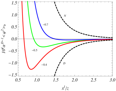
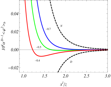
Figure 1: The boundary-induced part in the VEV of the field squared versus the proper distance from the brane for $D=4$ conformally (left panel) and minimally (right panel) coupled scalar fields with $m\alpha=0.5$. The numbers near the solid curves correspond to the values of the ratio $\beta/z$ and the dashed curves are for Dirichlet and Neumann boundary conditions.

4 Vacuum energy density and stresses

Having the Wightman function and the mean field squared, the VEV of the energy-momentum tensor is evaluated by making use of the formula

$$\langle T_{ik}\rangle=\lim_{x^{\prime}\rightarrow x}\partial_{i}\partial_{k}^{\prime}W(x,x^{\prime})+\left[\left(\xi-1/4\right)g_{ik}\nabla_{l}\nabla^{l}-\zeta\nabla_{i}\nabla_{k}-\zeta R_{ik}\right]\langle\varphi^{2}\rangle,$$ (42)

where $R_{ik}=-Dg_{ik}/\alpha^{2}$ is the Ricci tensor for AdS spacetime. In defining the right-hand side of this formula we have used the expression for the energy-momentum tensor for a scalar field which differs from the standard one (given, for example, in [13]) by a term that vanishes on the solutions of the field equation (see [24]). Similar to the VEV of the field squared, the vacuum energy-momentum tensor is decomposed into boundary-free and boundary-induced parts:

$$\langle T_{ik}\rangle=\langle T_{ik}\rangle_{0}+\langle T_{ik}\rangle_{b}.$$ (43)

As a consequence of the maximal symmetry of boundary-free AdS spacetime and of the vacuum state under consideration, one has $\langle T_{ik}\rangle_{0}=\mathrm{const}\cdot g_{ik}$. Hence, the corresponding vacuum energy-momentum tensor is completely determined by its trace. The boundary-free energy-momentum tensor $\langle T_{ik}\rangle_{0}$ is well investigated in the literature (see, for instance, [16]) and in what follows we shall be concerned with the brane-induced contribution, $\langle T_{ik}\rangle_{b}$.

For the covariant d’Alembertian acted on the brane-induced part of the field squared we find

$$\nabla_{l}\nabla^{l}\langle\varphi^{2}\rangle_{b}=-\frac{2^{-2\nu-1}\alpha^{-D-1}}{\left(4\pi\right)^{(D-1)/2}}\int_{0}^{\infty}dx\,xe^{-2xx^{1}/z}\frac{\beta x/z+1}{\beta x/z-1}\hat{B}(x)x^{D+2\nu}F_{\nu}^{D/2}(x),$$ (44)

with the differential operator

$$\hat{B}(x)=\partial_{x}^{2}-\frac{D-1}{x}\partial_{x}+4.$$ (45)

By making use of the expressions for the boundary-induced contributions in the Wightman function and in the VEV of the field squared, Eq. (32), from (42) for the diagonal components in the region $x^{1}>0$ one gets (no summation over $i=0,1,\ldots,D$)

$$\langle T_{i}^{i}\rangle_{b} = -\frac{\left(4\pi\right)^{(1-D)/2}}{2^{2\nu+1}\alpha^{D+1}}\int_{0}^{\infty}dx\,xe^{-2xx^{1}/z}\frac{\beta x/z+1}{\beta x/z-1}$$ (46)

$$\times\left[A_{i}x^{D+2\nu}F_{\nu}^{D/2+1}(x)+\hat{B}_{i}(x)x^{D+2\nu}F_{\nu}^{D/2}(x)\right],$$

with the notations

$$A_{i} = 1/2,\;i=0,2,\ldots,D-1,$$

$$A_{1} = 0,\;A_{D}=\frac{1-D}{2},$$ (47)

and

$$\hat{B}_{i}(x) = \frac{\xi_{1}}{4}\hat{B}(x)+\frac{\xi}{x}\partial_{x}-\frac{\xi D}{x^{2}},\;i=0,2,\ldots,D-1,$$

$$\hat{B}_{1}(x) = \frac{\xi_{1}}{4}\hat{B}(x)+\frac{\xi}{x}\partial_{x}-\frac{\xi D}{x^{2}}-\xi_{1},$$ (48)

$$\hat{B}_{D}(x) = \frac{1}{4}\hat{B}(x)-\xi\frac{D}{x}\partial_{x}+\xi_{1}+\frac{D^{2}\xi-m^{2}\alpha^{2}}{x^{2}}.$$

Here and in what follows, we use the notation $\xi_{1}=4\xi-1$. The diagonal components are symmetric under the reflection $x^{1}\rightarrow-x^{1}$ with respect to the brane: they are given by the expression (46) with $x^{1}$ replaced by $|x^{1}|$. The vacuum stresses along the directions parallel to the brane are equal to the energy density. This property is a consequence of the invariance with respect to the Lorentz boosts along those directions.

In addition to the diagonal components, the vacuum energy-momentum tensor has off-diagonal components $\langle T_{D}^{1}\rangle_{b}=\langle T_{1}^{D}\rangle_{b}$. For the latter one gets

$$\langle T_{D}^{1}\rangle_{b}=\frac{\left(4\pi\right)^{(1-D)/2}}{2^{2\nu}\alpha^{D+1}}\int_{0}^{\infty}dx\,e^{-2xx^{1}/z}\frac{\beta x/z+1}{\beta x/z-1}\left[\left(\frac{1}{4}-\xi\right)x\partial_{x}-\xi\right]x^{D+2\nu}F_{\nu}^{D/2}(x).$$ (49)

This off-diagonal component changes the sign under the reflection $x^{1}\rightarrow-x^{1}$. Similar to the case of the field squared, the mean energy-momentum tensor depends on the coordinates $x^{1}$, $z$, and on the parameter $\beta$ in the form of the ratios $x^{1}/z$ and $\beta/z$. The first of these is the proper distance from the brane measured in units of the curvature radius $\alpha$. Note that for the derivatives appearing in (46) and (49) one has the relations

$$\partial_{x}[x^{D+2\nu}F_{\nu}^{D/2}(x)] = x^{D+2\nu-1}[F_{\nu}^{D/2}(x)+2F_{\nu}^{D/2-1}(x)],$$

$$\partial_{x}^{2}[x^{D+2\nu}F_{\nu}^{D/2}(x)] = 2x^{D+2\nu-2}[3F_{\nu}^{D/2-1}(x)+2F_{\nu}^{D/2-2}(x)].$$ (50)

Here we have used the formula $\partial_{z}\left[z^{b}\,_{1}F_{2}\left(a;b+1,2a;z\right)\right]=bz^{b-1}\,_{1}F_{2}\left(a;b,2a;z\right)$ with $a=\nu+1/2$.

By using the expressions given above, we can see that the boundary-induced contributions obey the trace relation

$$\langle T_{i}^{i}\rangle_{b}=D\left(\xi-\xi_{D}\right)\nabla_{l}\nabla^{l}\langle\varphi^{2}\rangle_{b}+m^{2}\langle\varphi^{2}\rangle_{b}.$$ (51)

In particular, the brane-induced part is traceless for a conformally coupled massless field. The trace anomalies are contained in the boundary-free part only. As an additional check for the expressions given above, we can see that the covariant continuity equation $\nabla_{k}\langle T_{i}^{k}\rangle_{b}=0$ is obeyed. For the geometry under consideration the latter is reduced to the following relations

$$\partial_{1}\langle T_{1}^{1}\rangle_{b}+\partial_{D}\langle T_{1}^{D}\rangle_{b}-\frac{D+1}{z}\langle T_{1}^{D}\rangle_{b} = 0,$$

$$\partial_{1}\langle T_{D}^{1}\rangle_{b}+\partial_{D}\langle T_{D}^{D}\rangle_{b}-\frac{D}{z}\langle T_{D}^{D}\rangle_{b}+\frac{1}{z}\sum_{k=0}^{D-1}\langle T_{k}^{k}\rangle_{b} = 0.$$ (52)

The Minkowskian limit for the VEVs of the energy-momentum tensor is considered in a way similar to that for the VEV of the field squared. By using the asymptotic expression (35), to the leading order for the diagonal components we get (nu summation over $i$) $\langle T_{i}^{i}\rangle_{b}\approx\langle T_{i}^{i}\rangle_{b}^{(M)}$, where for a plate in Minkowski spacetime one has (see [22])

$$\langle T_{i}^{i}\rangle_{b}^{(M)}=-\frac{\left(4\pi\right)^{-D/2}}{\Gamma(D/2)}\int_{m}^{\infty}du\,e^{-2xx^{1}}\frac{\beta u+1}{\beta u-1}\left(u^{2}-m^{2}\right)^{D/2-1}\left[4\left(\xi-\xi_{D}\right)u^{2}-m^{2}/D\right],$$ (53)

for $i=0,2,\ldots,D$ and $\langle T_{1}^{1}\rangle_{b}^{(M)}=0$. For the leading term in the off-diagonal component we find

$$\langle T_{D}^{1}\rangle_{b} \approx -\frac{2\left(4\pi\right)^{-D/2}}{\Gamma(D/2)\alpha}\int_{0}^{\infty}du\,ue^{-2ux^{1}}\frac{\beta u+1}{\beta u-1}\left(u^{2}-m^{2}\right)^{D/2-2}$$ (54)

$$\times\left[D\left(\xi-\xi_{D}\right)u^{2}+\left(1/4-2\xi\right)m^{2}\right],$$

and it vanishes in the Minkowskian limit. Note that for the normal stress one has $\langle T_{1}^{1}\rangle_{b}=\mathcal{O}(1/\alpha^{2})$. For a conformally coupled massless field, the Minkowskian limit of the VEV of the energy-momentum tensor vanishes for a single plate.

In the case of Dirichlet and Neumann boundary conditions it is convenient to evaluate the VEV of the energy-momentum tensor by using the formula (42) with the Wightman function from (18). For the boundary-induced contributions in the diagonal components we find (no summation over $i$)

$$\langle T_{i}^{i}\rangle_{b}=\pm\frac{\pi^{-D/2}\alpha^{-D-1}}{2^{D/2+\nu+1}}[\hat{C}_{i}(u)-D\xi]f_{\nu}(u),$$ (55)

where, as before, the upper/lower sign corresponds to Dirichlet/Neumann boundary condition and $u$ is defined in accordance with (34). In (55), $\hat{C}_{i}(u)$ are the second order differential operators defined by the expressions ($i=0,2,\ldots,D-1$)

$$\hat{C}_{i}(u) = \xi_{1}\left(u^{2}-1\right)\partial_{u}^{2}+\left[4\xi-2+\left(\frac{D+1}{2}\xi_{1}-\frac{1}{2}\right)\left(u-1\right)\right]\partial_{u},$$

$$\hat{C}_{1}(u) = \xi_{1}\left(u-1\right)^{2}\partial_{u}^{2}+\left(\frac{D+1}{2}\xi_{1}-\frac{1}{2}\right)\left(u-1\right)\partial_{u},$$

$$\hat{C}_{D}(u) = 2\xi_{1}\left(u-1\right)\partial_{u}^{2}+\left[4\xi-2+\frac{D}{2}\xi_{1}\left(u-1\right)\right]\partial_{u},$$ (56)

with $\xi_{1}=4\xi-1$. For the off-diagonal component one gets

$$\langle T_{D}^{1}\rangle_{b}=\pm\frac{2\alpha^{-D-1}x^{1}/z}{2^{D/2+\nu+1}\pi^{D/2}}\left[\xi_{1}\left(u-1\right)\partial_{u}^{2}+\left(2\xi-1\right)\partial_{u}\right]f_{\nu}(u).$$ (57)

The second derivatives in (55) and (57) can be excluded by using the differential equation for the function $f_{\nu}(u)$. The latter is obtained by using the definition (15) and the equation for the function $\,{}_{2}F_{1}$. In this way we can see that

$$[\left(u^{2}-1\right)\partial_{u}^{2}+\left(D+1\right)u\partial_{u}+D^{2}/4-\nu^{2}]f_{\nu}(u)=0.$$ (58)

As an additional check, by making use of (58), it can be shown that the VEVs (55) and (57) obey the trace relation (51).

Let us consider the asymptotic behavior of the vacuum energy-momentum tensor near the brane and at large distances for general case of Robin boundary condition. For points near the brane, $x^{1}/z\ll 1$, the dominant contribution to the integral in (46) comes from large values of $x$. The corresponding asymptotic of the function $F_{\nu}^{\mu}(x)$ was given by (37). Assuming that $x^{1}/|\beta|\ll 1$, in the leading order we find (no summation over $i=0,2,\ldots,D$)

$$\langle T_{i}^{i}\rangle_{b} \approx \frac{2D\left(\xi_{D}-\xi\right)\Gamma((D+1)/2)}{\pi^{(D+1)/2}\left(2\alpha x^{1}/z\right)^{D+1}},$$

$$\langle T_{1}^{1}\rangle_{b} \approx -\frac{D\left(\xi_{D}-\xi\right)\Gamma((D-1)/2)}{4\pi^{(D+1)/2}\left(2\alpha x^{1}/z\right)^{D-1}},$$ (59)

for the diagonal components and

$$\langle T_{D}^{1}\rangle_{b}\approx\frac{D\left(\xi_{D}-\xi\right)\Gamma((D+1)/2)}{\pi^{(D+1)/2}\alpha(2\alpha x^{1}/z)^{D}},$$ (60)

for the off-diagonal component. For Dirichlet boundary condition ($\beta=0$) the asymptotic expressions are given by (59) and (60) with the opposite signs. For fixed $x^{1}$, the expressions in (59) and (60) give the leading terms near the AdS horizon. In particular, from (59) it follows that the energy density diverges on the horizon as $z^{D+1}$. Note that in the evaluation of the total energy induced by the brane, $E_{b}=\int d^{D}x\,\sqrt{|g|}\langle T_{0}^{0}\rangle_{b}$, an additional factor $1/z^{D+1}$ comes from the volume element.

At large distances from the brane, $x^{1}/z\gg 1$, the main contribution to the integrals in (46) and (49) comes from the region near the lower limit of the integration. Assuming that $|\beta|/x^{1}\ll 1$, for the diagonal components we get (no summation over $i$)

$$\langle T_{i}^{i}\rangle_{b}\approx\frac{\alpha^{-D-1}B_{i}\Gamma(D/2+\nu)}{\pi^{D/2}\Gamma(\nu)(2x^{1}/z)^{D+2\nu}},$$ (61)

where $B_{i}=\left(\xi-1/4\right)\left(D+2\nu\right)+\xi$ for $i=0,\ldots,D-1$, and $B_{D}=-DB_{0}/(2\nu)$. For the off-diagonal component one finds

$$\langle T_{D}^{1}\rangle_{b}\approx\frac{2\alpha^{-D-1}B_{0}\Gamma(D/2+\nu+1)}{\pi^{D/2}\Gamma(1+\nu)\left(2x^{1}/z\right)^{D+2\nu+1}}.$$ (62)

As is seen, at large distances the off-diagonal component is suppressed by an additional factor $x^{1}/z$. For Neumann boundary condition, $\beta=0$, the asymptotics at large distances are given by the expressions (61) and (62) with the opposite signs. As in the case of the field square, at large distances one has a power-law decay instead of exponential one for the problem with a massive field in Minkowski bulk. From (61) and (62) it follows that, for fixed $x^{1}$, the diagonal components vanish on the AdS boundary as $z^{D+2\nu}$. The integrand in the expression for the total energy induced by the brane, $E_{b}$, near the horizon behaves like $z^{2\nu-1}$ and the integral over $z$ converges at $z=0$ for $\nu>0$.

The figure 2 displays the boundary-induced part in the VEV of the energy density for the cases of $D=4$ conformally (left panel) and minimally (right panel) coupled scalar fields as a function of the ration $x^{1}/z$ (proper distance from the brane measured in units of the AdS curvature radius). The dashed lines correspond to Dirichlet and Neumann boundary conditions. The numbers near the solid curves correspond to the values of the ratio $\beta/z$. The graphs are plotted for $m\alpha=0.5$.

.

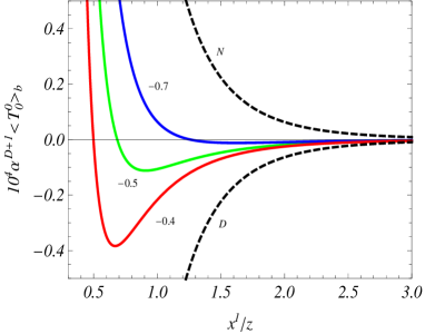
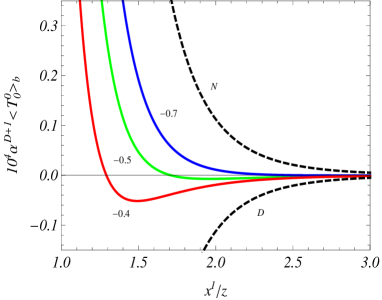
Figure 2: The vacuum energy density induced by a brane as a function of the proper distance measured in units of the AdS curvature radius. The graphs are plotted for $D=4$ conformally (left panel) and minimally (right panel) coupled scalar fields with $m\alpha=0.5$. Dashed curves correspond to Dirichlet and Neumann boundary conditions and the numbers near the solid curves are the values of the ratio $\beta/z$.

5 Conclusion

In the present paper we have investigated quantum effects induced by a flat brane for a scalar field in background of AdS spacetime. The brane is perpendicular to the AdS boundary and the field operator obeys Robin boundary condition on it. We consider a free field theory in AdS spacetime and all the information on the vacuum state is contained in the two-point functions. As such a function, the positive-frequency Wightman function is chosen, which also determines the response of the Unruh-DeWitt-type particle detectors. We have provided an expression for the Wightman function in which the contribution induced by the brane is explicitly separated from the pure AdS one and is given by the second term in the right-hand side of (17). This allows to reduce the renormalization procedure for the local VEVs, at points away from the brane, to the one in AdS spacetime in the absence of the brane. The latter problem is well discussed in the literature. The expression for the Wightman function is further simplified in special cases of Dirichlet and Neumann boundary conditions and is given by (18). For a fixed value of the proper distance from the brane, near the AdS boundary, the Neumann boundary condition is an ”attractor” in the general class of Robin boundary conditions, whereas Dirichlet boundary condition is an ”attractor” near the horizon. We have also evaluated the bulk-to-boundary propagator which plays an important role in the discussions of the AdS/CFT correspondence. Similar to the case of the Wightman function, the corresponding expression is decomposed into the boundary-free and brane-induced contributions.

As an important characteristic of the quantum vacuum, in section 3 we have studied the mean field squared. The brane-induced contribution in this VEV is presented in the form (32) where the function $F_{\nu}^{\mu}(x)$ is defined by (31). This contribution depends on the coordinates $x^{1}$, $z$ and on the paramater $\beta$ in the Robin boundary condition in the form of the ratios $x^{1}/z$ and $\beta/z$. This property is a consequence of the maximal symmetry of AdS spacetime. For Dirichlet and Neumann boundary conditions the integral in (32) is expressed in terms of the hypergeometric function and the corresponding formula simplifies to (33). As an additional check of the results derived, we have shown that in the limit $\alpha\rightarrow\infty$ the corresponding expression for a Robin plate in Minkowski spacetime is obtained. The boundary-induced VEV diverges on the brane with the leading term given by (39) for non-Dirichlet boundary conditions. For Dirichlet boundary condition the leading term has the opposite sign. For points near the brane, the influence of the gravitational field on the VEV is small and the leading term coincides with that in Minkowski spacetime. The influence of gravity is crucial at the proper distances from the brane larger than the AdS curvature radius. In this limit, for non-Neumann boundary conditions the leading term in the corresponding asymptotic expansion has the form (41). For Neumann boundary condition the same expression is obtained with the opposite sign. For AdS bulk the decay of the boundary-induced contribution at large distances from the brane is power-law for both massless and massive fields. This is in clear contrast with the case of the problem in Minkowski spacetime, where the boundary-induced VEV for a massive field decays exponentially. For a given $x^{1}$, the brane-induced contribution in the VEV of the field squared vanishes on the AdS boundary as $z^{D+2\nu}$ and diverges on the horizon like $z^{D-1}$.

Another important quantity, characterizing the vacuum fluctuations in the presence of the brane, is the VEV of the energy-momentum tensor. The boundary-induced contributions in the diagonal components are given by (46). The vacuum stresses along the directions parallel to the brane are equal to the energy density. In addition to the diagonal components the vacuum energy-momentum tensor has an off-diagonal component defined by the expression (49). The formulas for the components of the vacuum energy-momentum tensor are further simplified for the cases of Dirichlet and Neumann boundary conditions (see (55) and (57)). We have explicitly checked that the brane-induced parts obey the trace relation (51) and the covariant conservation equation. The latter is reduced to the relations (52). In the limit of large values for the AdS curvature radius, to the leading order, for the energy density and parallel stresses we obtain the corresponding result in Minkowski bulk. In this limit, the off diagonal component and the normal stress behave like $\langle T_{D}^{1}\rangle_{b}\propto 1/\alpha$ and $\langle T_{1}^{1}\rangle_{b}\propto 1/\alpha^{2}$. For proper distances from the brane smaller than the AdS curvature radius, with an additional assumption that $x^{1}/|\beta|\ll 1$, the leading terms in the asymptotic expansion over the distance are given by (59), (60) for non-Dirichlet boundary conditions. For Dirichlet boundary condition the leading asymptotic is given by the same expressions with the opposite sign. The leading terms vanish for a conformally coupled field and in this case the divergences on the brane are weaker. At large proper distances from the brane and for non-Neumann boundary conditions, the diagonal components of the vacuum energy-momentum tensor decay like $(z/x^{1})^{D+2\nu}$ and the off-diagonal component behaves as $(z/x^{1})^{D+2\nu+1}$. In the case of Neumann boundary condition the asymptotics have the opposite sign. For fixed $x^{1}$, the diagonal components decay on the AdS boundary as $z^{D+2\nu}$ and diverge on the horizon as $z^{D+1}$.

References

- [1] J. M. Maldacena, Adv. Theor. Math. Phys. 2, 231 (1998); S.S. Gubser, I.R. Klebanov and A. M. Polyakov, Phys. Lett. B 428, 105 (1998); E. Witten, Adv. Theor. Math. Phys. 2, 253 (1998).
- [2] O. Aharony, S.S. Gubser, J. Maldacena, H. Ooguri and Y. Oz, Phys. Rep. 323 183 (2000).
- [3] V.A. Rubakov, Phys. Usp. 44, 871 (2001); P. Brax and C. Van de Bruck, Class. Quantum Grav. 20, R201 (2003); R. Maartens and K. Koyama, Living Rev. Rel. 13, 5 (2010).
- [4] E. Elizalde, S.D. Odintsov, A. Romeo, A.A. Bytsenko, and S. Zerbini, Zeta Regularization Techniques with Applications (World Scientific, Singapore, 1994); V.M. Mostepanenko and N.N. Trunov, The Casimir Effect and its Applications (Clarendon, Oxford, 1997); K.A. Milton, The Casimir Effect: Physical Manifestation of Zero-Point Energy (World Scientific, Singapore, 2002); M. Bordag, G.L. Klimchitskaya, U. Mohideen, and V.M. Mostepanenko, Advances in the Casimir Effect (Oxford University Press, Oxford, 2009); Casimir Physics, edited by D. Dalvit, P. Milonni, D. Roberts, and F. da Rosa, Lecture Notes in Physics Vol. 834 (Springer-Verlag, Berlin, 2011).
- [5] M. Fabinger and P. Horava, Nucl. Phys. B 580, 243 (2000); W. Goldberger and I. Rothstein, Phys. Lett. B 491, 339 (2000); S. Nojiri, S.D. Odintsov, and S. Zerbini, Class. Quantum Grav. 17, 4855 (2000); I. Brevik, K.A. Milton, S. Nojiri, and S.D. Odintsov, Nucl. Phys. B 599, 305 (2001); A. Flachi, I.G. Moss, and D.J. Toms, Phys. Lett. B 518, 153 (2001); J. Garriga, O. Pujolàs, and T. Tanaka, Nucl. Phys. B 605, 192 (2001); A. Flachi, I.G. Moss, and D.J. Toms, Phys. Rev. D 64, 105029 (2001); A. Flachi and D.J. Toms, Nucl. Phys. B 610, 144 (2001); A.A. Saharian and M.R. Setare, Phys. Lett. B 552, 119 (2003); J. Garriga and A. Pomarol, Phys. Lett. B 560, 91 (2003); E. Elizalde, S. Nojiri, S.D. Odintsov, and S. Ogushi, Phys. Rev. D 67, 063515 (2003); A.A. Saharian and M.R. Setare, Phys. Lett. B 584, 306 (2004); A. Flachi, A. Knapman, W. Naylor, and M. Sasaki, Phys. Rev. D 70, 124011 (2004); E. Elizalde, S. Nojiri, and S.D. Odintsov, Phys. Rev. D 70, 043539 (2004); M. R. Setare, Eur. Phys. J. C 38, 373 (2004); E. Elizalde, S. Nojiri, S.D. Odintsov, and P. Wang, Phys. Rev. D 71, 103504 (2005); M. Frank, I. Turan, and L. Ziegler, Phys. Rev. D 76, 015008 (2007); E. Elizalde, S.D. Odintsov, and A.A. Saharian, Phys. Rev. D 79, 065023 (2009); L.P. Teo, Phys. Lett. B 682, 259 (2009); A. Flachi and T. Tanaka, Phys. Rev. D 80, 124022 (2009); M. Rypestøl and I. Brevik, New J. Phys 12, 013022 (2010).
- [6] A. Knapman and D.J. Toms, Phys. Rev. D 69, 044023 (2004); A.A. Saharian, Nucl. Phys. B 712, 196 (2005); A.A. Saharian, Phys. Rev. D 70, 064026 (2004); S.-H. Shao, P. Chen, and J.-A. Gu, Phys. Rev. D 81, 084036 (2010); E. Elizalde, S.D. Odintsov, and A.A. Saharian, Phys. Rev. D 87, 084003 (2013).
- [7] A. Flachi, J. Garriga, O. Pujolàs, and T. Tanaka, J. High Energy Phys. 08 (2003) 053; A. Flachi and O. Pujolàs, Phys. Rev. D 68, 025023 (2003); A.A. Saharian, Phys. Rev. D 73, 044012 (2006); A.A. Saharian, Phys. Rev. D 73, 064019 (2006); A.A. Saharian, Phys. Rev. D 74, 124009 (2006); E. Elizalde, M. Minamitsuji, and W. Naylor, Phys. Rev. D 75, 064032 (2007); R. Linares, H.A. Morales-Técotl, and O. Pedraza, Phys. Rev. D 77, 066012 (2008); M. Frank, N. Saad, and I. Turan, Phys. Rev. D 78, 055014 (2008); E.R. Bezerra de Mello, A.A. Saharian, V. Vardanyan, Phys. Lett. B 741, 155 (2015).
- [8] E.R. Bezerra de Mello and A.A. Saharian, J. Phys. A: Math. Theor. 45, 115402 (2012); E.R. Bezerra de Mello, E.R. Figueiredo Medeiros, and A.A. Saharian, Class. Quantum Grav. 30, 175001 (2013).
- [9] T. Takayanagi, Phys. Rev. Lett. 107, 101602 (2011); M. Fujita, T. Takayanagi, and E. Tonni, JHEP 11 (2011) 043.
- [10] S. Ryu and T. Takayanagi, Phys. Rev. Lett. 96, 181602 (2006); S. Ryu and T. Takayanagi, JHEP 08 (2006) 045.
- [11] T. Nishioka, S. Ryu, and T. Takayanagi, J. Phys. A: Math. Theor. 42, 504008 (2009).
- [12] T. Gherghetta and A. Pomarol, Nucl. Phys. B 586, 141 (2000).
- [13] N.D. Birrell and P.C.W. Davis, Quantum Fields in Curved Space (Cambridge University Press, Cambridge, 1982).
- [14] P. Breitenlohner and D. Z. Freedman, Ann. Phys. (N.Y.) 144, 249 (1982); L. Mezincescu and P.K. Townsend, Ann. Phys. (N.Y.) 160, 406 (1985).
- [15] C.P. Burgess and C.A. Lütken, Phys. Lett. B 153, 137 (1985).
- [16] R. Camporesi and A. Higuchi, Phys. Rev. D 45, 3591 (1992).
- [17] D.Z. Freedman, S.D. Mathur, A. Matusis, and L. Rastelli, Nucl. Phys. B 546, 96 (1999); I.R. Klebanov and E. Witten, Nucl. Phys. B 556, 89 (1999).
- [18] M. Alishahiha and R. Fareghbal, Phys. Rev. D 84, 106002 (2011); K. Hinterbichler, J. Stokes, and M. Trodden, Phys. Rev. D 92, 065025 (2015).
- [19] M. Kamela, C.P. Burgess, Can. J. Phys. 77, 85 (1999).
- [20] M.M. Caldarelli, Nucl. Phys. B 549, 499 (1999).
- [21] A.P. Prudnikov, Yu.A. Brychkov, and O.I. Marichev, Integrals and Series, Vol.2 (Gordon and Breach, New York, 1986).
- [22] A. Romeo and A.A. Saharian, J. Phys. A: Math. Gen. 35, 1297 (2002); A.A. Saharian, The Generalized Abel-Plana Formula with Applications to Bessel Functions and Casimir Effect (Yerevan State University Publishing House, Yerevan, 2008); Report No. ICTP/2007/082; arXiv:0708.1187.
- [23] A.A. Saharian and T.A. Vardanyan, Class. Quantum Grav. 26, 195004 (2009).
- [24] A.A. Saharian, Phys. Rev. D 69, 085005 (2004).