Collaborative Compressive Detection with Physical Layer Secrecy Constraints

Bhavya Kailkhura, , Thakshila Wimalajeewa, , Pramod K. Varshney This work was supported in part by the National Science Foundation (NSF) under Grant No. 1307775.Some related preliminary work was presented at the Forty Eighth Asilomar Conf. on Signals, Systems and Computers, Nov 2014. Authors are with Department of EECS, Syracuse University, Syracuse, NY 13244. (email: bkailkhu@syr.edu; twwewelw@syr.edu; varshney@syr.edu).
Abstract

This paper considers the problem of detecting a high dimensional signal (not necessarily sparse) based on compressed measurements with physical layer secrecy guarantees. First, we propose a collaborative compressive detection (CCD) framework to compensate for the performance loss due to compression with a single sensor. We characterize the trade-off between dimensionality reduction achieved by a universal compressive sensing (CS) based measurement scheme and the achievable performance of CCD analytically. Next, we consider a scenario where the network operates in the presence of an eavesdropper who wants to discover the state of the nature being monitored by the system. To keep the data secret from the eavesdropper, we propose to use cooperating trustworthy nodes that assist the fusion center (FC) by injecting artificial noise to deceive the eavesdropper. We seek the answers to the questions: Does CS help improve the security performance in such a framework? What are the optimal values of parameters which maximize the CS based collaborative detection performance at the FC while ensuring perfect secrecy at the eavesdropper?

Index Terms:
Compressive detection, dimensionality reduction, compressive sensing, random projections, artificial noise injection, eavesdropper, secrecy.

I Introduction

Compressive sensing (CS) is a new paradigm which enables the reconstruction of compressible or sparse signals using far fewer samples than required by the Nyquist criterion [1, 2]. In this framework, a small collection of linear random projections of a sparse signal contains sufficient information for signal recovery. To reconstruct the original signal from its compressed measurements, several algorithms have been proposed in the literature [3].

While CS mostly deals with complete signal reconstruction, there are several signal processing applications where complete signal recovery is not necessary. Instead we might be only interested in solving inference problems such as detection, classification or estimation of certain parameters. To solve an inference problem where some prior information about the signal is available, a customized measurement scheme could be implemented such that the optimal inference performance is achieved for the particular signal. As an example, for a signal detection problem where the signal of interest is known, the optimal design is the matched filter which is dependent on the signal itself. However, it is possible that the signal that we wish to infer about may evolve over time. Thus, we are often interested in universal or agnostic design. A few attempts have been made in this direction to address the problems of inference in Compressive Signal Processing (CSP) literature in recent research [4, 5, 6]. CSP techniques are universal and agnostic to the signal structure and provide deterministic guarantees for a wide variety of signal classes.

The authors in [4, 7, 8] considered the deterministic signal detection problem in the compressed measurement domain where the performance limits of detection with compressed measurements were investigated. For signals that are not necessarily sparse, it was shown that a certain performance loss will be incurred due to compression when compared to the optimal test that acquires original measurements using the traditional measurement scheme. For stochastic signals, the compressive detection problem (i.e., detecting stochastic signals in the compressed measurement domain) was considered in [6, 9]. Both works focused only on compressive detection of ‘zero-mean’ stochastic signals based on observations corrupted by additive noise. Closed form expressions were derived for performance limits and performance loss due to compression was characterized analytically. A signal classification problem based on compressed measurements was considered in [10] where the authors developed a manifold based model for compressive classification. The authors in [11, 12] studied the performance of compressive sampling in detection and classification setup and introduced the generalized restricted isometry property that states that the angle between two vectors is preserved under random projections. Sparse event detection by sensor networks under a CS framework was considered in [13]. The problem of detection of spectral targets based on noisy incoherent projections was addressed in [14]. Schemes for the design and optimization of projection matrices for signal detection with compressed measurements have been proposed in [15, 16, 17, 18].

As mentioned earlier, CSP techniques are universal and agnostic to the signal structure and, therefore, are attractive in many practical applications. Despite its attractiveness to solve high dimensional inference problems, CSP suffers from a few major drawbacks which limit its applicability in practice. A CS based measurement scheme incurs a certain performance loss due to compression when compared to the traditional measurement scheme while detecting non sparse signals. This can be seen as the price one pays for universality in terms of inference performance. In this paper, we propose a collaborative compressive detection (CCD) framework to compensate for the performance loss due to compression. The CCD framework comprises of a group of spatially distributed nodes which acquire vector observations regarding the phenomenon of interest. Nodes send a compressed summary of their observations to the Fusion Center (FC) where a global decision is made. In this setup, we characterize the trade-off between dimensionality reduction in a universal CS based measurement scheme and the achievable performance. In our preliminary work [19], we analyzed the problem only for the deterministic signal case. In the current work, we significantly extend our previous work and investigate the problem for two different cases: 1)1) when the signal of interest is deterministic and 2)2) when the signal of interest is random. It is worthwhile to point out that, in contrast to [6, 9] where compressive detection of ‘zero-mean’ stochastic signals was considered, we study a more general problem with ‘non zero-mean’ stochastic signals. Note that, some of these existing results can be seen as a special case of analytical results derived in this paper. For both the cases, we show that for a fixed signal to noise ratio (SNR), if the number of collaborating nodes is greater than (1/c)1𝑐(1/c), where 0c10𝑐10\leq c\leq 1 is the compression ratio, the loss due to compression can be recovered.

In a CCD framework, the FC receives compressive observation vectors from the nodes and makes the global decision about the presence of the signal vector. The transmissions by the nodes, however, may be observed by an eavesdropper. The secrecy of a detection system against eavesdropping attacks is of utmost importance [20]. In a fundamental sense, there are two motives for any eavesdropper (Eve), namely selfishness and maliciousness, to compromise the secrecy of a given inference network. For instance, some of the nodes within a cognitive radio network (CRN) may selfishly take advantage of the FC’s inferences and may compete against the CRN in using the primary user’s channels without paying any participation costs to the network moderator. In another example, if the radar decisions are leaked to a malicious aircraft, the adversary aircraft can maliciously adapt its strategy against a given distributed radar network accordingly so as to remain invisible to the radar and in clandestine pursuit of its mission. Therefore, in the recent past, there has been a lot of interest in the research community in addressing eavesdropping attacks on inference networks. Recently, a few attempts have been made to address the problem of eavesdropping threats on distributed detection network. However, a similar study in a CSP framework is missing from the literature.

Next, we investigate the CCD problem when the network operates in the presence of an eavesdropper who wants to discover the state of the nature being monitored by the system. While security issues with CS based measurement schemes have been considered in [21, 22, 23], our work is considerably different. In contrast to [21, 22, 23], where performance limits of secrecy of CS based measurement schemes were analyzed (under different assumptions), we look at the problem from a practical perspective. We pursue a more active approach where the problem of optimal system design with secrecy guarantees is studied in an optimization setup. More specifically, we propose to use cooperating trustworthy nodes that assist the FC by injecting artificial noise to deceive the eavesdroppers to improve the security performance of the system. The addition of artificial noise to node transmissions is a data falsification scheme that is employed to confuse the eavesdropper. We consider the problem of determining optimal system parameters which maximize the detection performance at the FC, while ensuring perfect secrecy at the eavesdropper (information of the eavesdropper is exactly zero). In the process of determining optimal system parameters, we seek the answer to the question: Does compression help in improving the security performance of the system? At first glance, it seems intuitive that compression should always improve the security performance. However, we show that this argument is not necessarily true. In fact, security performance of the system is independent of the compression ratio in the perfect secrecy regime.

I-A Main Contributions

Our work presented in this paper is motivated by a number of factors. First, CS based measurement schemes incur a certain performance loss due to compression when compared to traditional measurement schemes while detecting non sparse signals, and, therefore, techniques to mitigate this loss are desirable. Next, CSP has been proposed relatively recently and, therefore, security issues for such a framework have been left un-addressed so far. Also, most of the works on CSP mainly focus on deriving theoretical performance bounds under different contexts. Despite its theoretical importance, practical implications of these bounds for system design have not been investigated in literature. In this paper, we take some first steps in addressing these issues for solving high dimensional signal detection problems using only compressed measurements taking security aspects into consideration. The main contributions of this paper are summarized as follows.

  • We propose a collaborative compressive detection (CCD) framework to compensate for the performance loss due to compression.

  • We characterize the trade-off between dimensionality reduction in a universal compressive sensing based measurement scheme and the achievable performance of CCD analytically.

  • When the network operates in the presence of an eavesdropper, we employ artificial noise injection techniques to improve secrecy performance. Theoretical performance bounds for the scheme are also derived.

  • We consider the problem of determining optimal system parameters which maximize the detection performance at the FC, while ensuring perfect secrecy at the eavesdropper.

The rest of the paper is organized as follows. Section II presents the observation model and the problem formulation. In Section III, performance of collaborative compression detection is analyzed for both deterministic and random signal cases. In Section IV, we investigate the problem where the network operates in the presence of an eavesdropper and propose artificial noise injection techniques to improve secrecy performance. In Section V, we study the problem of determining optimal system parameters which maximize the detection performance at the FC, while ensuring perfect secrecy at the eavesdropper. Concluding remarks and possible future directions are given in Section VI.

II Collaborative Compressive Detection

Refer to caption
Figure 1: Collaborative Compressive Detection Network

II-A Observation Model

Consider two hypotheses H0subscript𝐻0H_{0} (signal is absent) and H1subscript𝐻1H_{1} (signal is present). Also, consider a parallel network, comprised of a central entity (known as the FC) and a set of N𝑁N nodes, which faces the task of determining which of the two hypotheses is true (see Figure 1). Prior probabilities of the two hypotheses H0subscript𝐻0H_{0} and H1subscript𝐻1H_{1} are denoted by P0subscript𝑃0P_{0} and P1subscript𝑃1P_{1}, respectively. The nodes observe the phenomenon (high dimensional signal), carry out local compression (low dimensional projection), and then send their local summary statistic to the FC. The FC makes a final decision after processing the locally compressed observations.

For the i𝑖ith node observed signal, uisubscript𝑢𝑖u_{i} can be modeled as

H0:ui=vi\displaystyle H_{0}\;:\quad u_{i}=v_{i}
H1:ui=s+vi\displaystyle H_{1}\;:\quad u_{i}=s+v_{i}

where uisubscript𝑢𝑖u_{i} is the P×1𝑃1P\times 1 observation vector, s𝑠s is either deterministic or random Gaussian signal vector (not necessarily sparse) to be detected. Specifically let s𝒩(μ,α1IP)similar-to𝑠𝒩𝜇superscript𝛼1subscript𝐼𝑃s\sim\mathcal{N}(\mu,\alpha^{-1}I_{P}) and additive noise vi𝒩(0,β1IP)similar-tosubscript𝑣𝑖𝒩0superscript𝛽1subscript𝐼𝑃v_{i}\sim\mathcal{N}(0,\beta^{-1}I_{P}) where x𝒩(μ,Σ)similar-to𝑥𝒩𝜇Σx\sim\mathcal{N}(\mu,\Sigma) denotes that the vector x𝑥x is distributed as multivariate Gaussian with mean vector μ𝜇\mu and the covariance matrix ΣΣ\Sigma, and IPsubscript𝐼𝑃I_{P} is the P×P𝑃𝑃P\times P identity matrix. Note that, the deterministic signal can be considered as a special case of the random signal s𝑠s with variance α1=0superscript𝛼10\alpha^{-1}=0. Observations at the nodes are assumed to be conditionally independent and identically distributed.

Each node sends a M𝑀M-length (<P)absent𝑃(<P) compressed version yisubscript𝑦𝑖y_{i} of its P𝑃P-length observation uisubscript𝑢𝑖u_{i} to the FC. The collection of M𝑀M-length universally sampled observations is given by, yi=ϕuisubscript𝑦𝑖italic-ϕsubscript𝑢𝑖y_{i}=\phi u_{i}, where ϕitalic-ϕ\phi is an M×P𝑀𝑃M\times P projection matrix, which is assumed to be the same for all the nodes, and yisubscript𝑦𝑖y_{i} is the M×1𝑀1M\times 1 compressed observation vector (local summary statistic).

Under the two hypotheses, the local summary statistic is

H0:yi=ϕvi\displaystyle H_{0}\;:\quad y_{i}=\phi v_{i}
H1:yi=ϕs+ϕvi.\displaystyle H_{1}\;:\quad y_{i}=\phi s+\phi v_{i}.

The FC receives compressed observation vectors, 𝐲=[y1,,yN]𝐲subscript𝑦1subscript𝑦𝑁\mathbf{y}=[y_{1},\cdots,y_{N}], from the nodes via error free communication channels and makes the global decision about the phenomenon.

II-B Binary Hypothesis Testing at the Fusion Center

We consider the detection problem in a Bayesian setup where the performance criterion at the FC is the probability of error. The FC makes the global decision about the phenomenon by considering the likelihood ratio test (LRT) which is given by

i=1Nf1(yi)f0(yi)H1H0P0P1.superscriptsubscriptproduct𝑖1𝑁subscript𝑓1subscript𝑦𝑖subscript𝑓0subscript𝑦𝑖subscriptsuperscriptgreater-than-or-less-thansubscript𝐻1subscript𝐻0subscript𝑃0subscript𝑃1\prod\limits_{i=1}^{N}\dfrac{f_{1}(y_{i})}{f_{0}(y_{i})}\quad\mathop{\stackrel{{\scriptstyle H_{1}}}{{\gtrless}}}_{H_{0}}\quad\dfrac{P_{0}}{P_{1}}. (1)

Notice that, under the two hypotheses we have the following probability density functions (PDFs);

f0(yi)=exp(12yiT(β1ϕϕT)1yi)|β1ϕϕT|1/2(2π)M/2,subscript𝑓0subscript𝑦𝑖12superscriptsubscript𝑦𝑖𝑇superscriptsuperscript𝛽1italic-ϕsuperscriptitalic-ϕ𝑇1subscript𝑦𝑖superscriptsuperscript𝛽1italic-ϕsuperscriptitalic-ϕ𝑇12superscript2𝜋𝑀2\displaystyle f_{0}(y_{i})=\frac{\exp(-\frac{1}{2}y_{i}^{T}(\beta^{-1}\phi\phi^{T})^{-1}y_{i})}{|\beta^{-1}\phi\phi^{T}|^{1/2}(2\pi)^{M/2}}, (2)
f1(yi)=exp(12(yiϕμ)T((α1+β1)ϕϕT)1(yiϕμ))|(α1+β1)ϕϕT|1/2(2π)M/2.subscript𝑓1subscript𝑦𝑖12superscriptsubscript𝑦𝑖italic-ϕ𝜇𝑇superscriptsuperscript𝛼1superscript𝛽1italic-ϕsuperscriptitalic-ϕ𝑇1subscript𝑦𝑖italic-ϕ𝜇superscriptsuperscript𝛼1superscript𝛽1italic-ϕsuperscriptitalic-ϕ𝑇12superscript2𝜋𝑀2\displaystyle f_{1}(y_{i})=\frac{\exp(-\frac{1}{2}(y_{i}-\phi\mu)^{T}((\alpha^{-1}+\beta^{-1})\phi\phi^{T})^{-1}(y_{i}-\phi\mu))}{|(\alpha^{-1}+\beta^{-1})\phi\phi^{T}|^{1/2}(2\pi)^{M/2}}. (3)

After plugging in (2) and (3) in (1) and taking logarithms on both sides, we obtain an equivalent test that simplifies to

α1β1i=1NyiT(ϕϕT)1yi+2i=1NyiT(ϕϕT)1μH1H0λsuperscript𝛼1superscript𝛽1superscriptsubscript𝑖1𝑁superscriptsubscript𝑦𝑖𝑇superscriptitalic-ϕsuperscriptitalic-ϕ𝑇1subscript𝑦𝑖2superscriptsubscript𝑖1𝑁superscriptsubscript𝑦𝑖𝑇superscriptitalic-ϕsuperscriptitalic-ϕ𝑇1𝜇subscriptsuperscriptgreater-than-or-less-thansubscript𝐻1subscript𝐻0𝜆\frac{\alpha^{-1}}{\beta^{-1}}\sum\limits_{i=1}^{N}y_{i}^{T}(\phi\phi^{T})^{-1}y_{i}+2\sum\limits_{i=1}^{N}y_{i}^{T}(\phi\phi^{T})^{-1}\mu\quad\mathop{\stackrel{{\scriptstyle H_{1}}}{{\gtrless}}}_{H_{0}}\quad\lambda

where λ=(α1+β1)[2logP0P1+NMlog(1+α1β1)]+N(ϕμ)T(ϕϕT)1ϕμ𝜆superscript𝛼1superscript𝛽1delimited-[]2subscript𝑃0subscript𝑃1𝑁𝑀1superscript𝛼1superscript𝛽1𝑁superscriptitalic-ϕ𝜇𝑇superscriptitalic-ϕsuperscriptitalic-ϕ𝑇1italic-ϕ𝜇\lambda=(\alpha^{-1}+\beta^{-1})\left[2\log\frac{P_{0}}{P_{1}}+NM\log\left(1+\frac{\alpha^{-1}}{\beta^{-1}}\right)\right]+N(\phi\mu)^{T}(\phi\phi^{T})^{-1}\phi\mu.

For simplicity, we assume that P0=P1subscript𝑃0subscript𝑃1P_{0}=P_{1}. The test statistic for the collaborative compressive detector can be written in a compact form as

Λ(𝐲)=α1β1i=1NΛ1(yi)+2i=1NΛ2(yi)Λ𝐲superscript𝛼1superscript𝛽1superscriptsubscript𝑖1𝑁subscriptΛ1subscript𝑦𝑖2superscriptsubscript𝑖1𝑁subscriptΛ2subscript𝑦𝑖\Lambda(\mathbf{y})=\frac{\alpha^{-1}}{\beta^{-1}}\sum\limits_{i=1}^{N}\Lambda_{1}(y_{i})+2\sum\limits_{i=1}^{N}\Lambda_{2}({y_{i}}) (4)

where Λ1(yi)=yiT(ϕϕT)1yisubscriptΛ1subscript𝑦𝑖superscriptsubscript𝑦𝑖𝑇superscriptitalic-ϕsuperscriptitalic-ϕ𝑇1subscript𝑦𝑖\Lambda_{1}(y_{i})=y_{i}^{T}(\phi\phi^{T})^{-1}y_{i} and Λ2(yi)=yiT(ϕϕT)1μsubscriptΛ2subscript𝑦𝑖superscriptsubscript𝑦𝑖𝑇superscriptitalic-ϕsuperscriptitalic-ϕ𝑇1𝜇\Lambda_{2}({y_{i}})=y_{i}^{T}(\phi\phi^{T})^{-1}\mu.

We would like to point out that the test statistic for the deterministic signal and random signal with zero mean cases can be seen as a special case of the above test statistic. More specifically, for the deterministic signal s𝑠s, the test statistic is given by Λ(𝐲)=i=1NΛ1(yi)Λ𝐲superscriptsubscript𝑖1𝑁subscriptΛ1subscript𝑦𝑖\Lambda(\mathbf{y})=\sum\limits_{i=1}^{N}\Lambda_{1}(y_{i}) and for the zero mean random signal the test statistic is given by Λ(𝐲)=i=1NΛ2(yi)Λ𝐲superscriptsubscript𝑖1𝑁subscriptΛ2subscript𝑦𝑖\Lambda(\mathbf{y})=\sum\limits_{i=1}^{N}\Lambda_{2}(y_{i}) which is consistent with [19] and [6].

III Performance Analysis of Collaborative Compressive Detection

First, we look at the deterministic signal case and characterize the performance of the collaborative compressive detector.

III-A Deterministic Signal Case

The optimal test at the FC can be written in a compact form as

i=1NyiT(ϕϕT)1ϕsH1H0λ,superscriptsubscript𝑖1𝑁superscriptsubscript𝑦𝑖𝑇superscriptitalic-ϕsuperscriptitalic-ϕ𝑇1italic-ϕ𝑠subscriptsuperscriptgreater-than-or-less-thansubscript𝐻1subscript𝐻0𝜆\sum\limits_{i=1}^{N}y_{i}^{T}(\phi\phi^{T})^{-1}\phi s\quad\mathop{\stackrel{{\scriptstyle H_{1}}}{{\gtrless}}}_{H_{0}}\quad\lambda,

with λ=N2sTϕT(ϕϕT)1ϕs𝜆𝑁2superscript𝑠𝑇superscriptitalic-ϕ𝑇superscriptitalic-ϕsuperscriptitalic-ϕ𝑇1italic-ϕ𝑠\lambda=\frac{N}{2}s^{T}\phi^{T}(\phi\phi^{T})^{-1}\phi s. The decision statistic for the collaborative compressive detector is given as

Λ(𝐲)=i=1NyiT(ϕϕT)1ϕs.Λ𝐲superscriptsubscript𝑖1𝑁superscriptsubscript𝑦𝑖𝑇superscriptitalic-ϕsuperscriptitalic-ϕ𝑇1italic-ϕ𝑠\Lambda(\mathbf{y})=\sum\limits_{i=1}^{N}y_{i}^{T}(\phi\phi^{T})^{-1}\phi s. (5)

We analytically characterize the performance of the collaborative compressive detector in terms of the probability of error which is defined as

PE=12PF+12(1PD)subscript𝑃𝐸12subscript𝑃𝐹121subscript𝑃𝐷\displaystyle P_{E}=\dfrac{1}{2}P_{F}+\dfrac{1}{2}(1-P_{D})

where, PF=P(Λ(𝐲)>λ|H0)subscript𝑃𝐹𝑃Λ𝐲conditional𝜆subscript𝐻0P_{F}=P(\Lambda(\mathbf{y})>\lambda|H_{0}) and PD=P(Λ(𝐲)>λ|H1)subscript𝑃𝐷𝑃Λ𝐲conditional𝜆subscript𝐻1P_{D}=P(\Lambda(\mathbf{y})>\lambda|H_{1}) is the probability of false alarm and the probability of detection, respectively. To simplify the notations, we define

P^=ϕT(ϕϕT)1ϕ^𝑃superscriptitalic-ϕ𝑇superscriptitalic-ϕsuperscriptitalic-ϕ𝑇1italic-ϕ\hat{P}=\phi^{T}(\phi\phi^{T})^{-1}\phi

as the orthogonal projection operator onto row space of ϕitalic-ϕ\phi. Using this notation, it is easy to show that

Λ(𝐲){𝒩(0,β1NP^s22),underH0𝒩(NP^s22,β1NP^s22)underH1similar-toΛ𝐲cases𝒩0superscript𝛽1𝑁superscriptsubscriptnorm^𝑃𝑠22undersubscript𝐻0missing-subexpression𝒩𝑁superscriptsubscriptnorm^𝑃𝑠22superscript𝛽1𝑁superscriptsubscriptnorm^𝑃𝑠22undersubscript𝐻1missing-subexpression\Lambda(\mathbf{y})\sim\left\{\begin{array}[]{rll}\mathcal{N}(0,\beta^{-1}N\|\hat{P}s\|_{2}^{2}),&\mbox{under}\ H_{0}\\ \mathcal{N}(N\|\hat{P}s\|_{2}^{2},\beta^{-1}N\|\hat{P}s\|_{2}^{2})&\mbox{under}\ H_{1}\end{array}\right.

where P^s22=sTϕT(ϕϕT)1ϕssuperscriptsubscriptnorm^𝑃𝑠22superscript𝑠𝑇superscriptitalic-ϕ𝑇superscriptitalic-ϕsuperscriptitalic-ϕ𝑇1italic-ϕ𝑠\|\hat{P}s\|_{2}^{2}=s^{T}\phi^{T}(\phi\phi^{T})^{-1}\phi s.

Thus, we have

PF=Q(N2P^s22Nβ1P^s2)=Q(12Nβ1P^s2)subscript𝑃𝐹𝑄𝑁2superscriptsubscriptnorm^𝑃𝑠22𝑁superscript𝛽1subscriptnorm^𝑃𝑠2𝑄12𝑁superscript𝛽1subscriptnorm^𝑃𝑠2P_{F}=Q\left(\frac{\frac{N}{2}\|\hat{P}s\|_{2}^{2}}{\sqrt{N\beta^{-1}}\|\hat{P}s\|_{2}}\right)=Q\left(\frac{1}{2}\sqrt{\frac{N}{\beta^{-1}}}\|\hat{P}s\|_{2}\right) (6)

and

PD=Q(N2P^s22NP^s22Nβ1P^s2)=Q(12Nβ1P^s2)subscript𝑃𝐷𝑄𝑁2superscriptsubscriptnorm^𝑃𝑠22𝑁superscriptsubscriptnorm^𝑃𝑠22𝑁superscript𝛽1subscriptnorm^𝑃𝑠2𝑄12𝑁superscript𝛽1subscriptnorm^𝑃𝑠2P_{D}=Q\left(\frac{\frac{N}{2}\|\hat{P}s\|_{2}^{2}-N\|\hat{P}s\|_{2}^{2}}{\sqrt{N\beta^{-1}}\|\hat{P}s\|_{2}}\right)=Q\left(-\frac{1}{2}\sqrt{\frac{N}{\beta^{-1}}}\|\hat{P}s\|_{2}\right) (7)

where Q(x)=12πxexp(u22)𝑑u𝑄𝑥12𝜋superscriptsubscript𝑥superscript𝑢22differential-d𝑢Q(x)=\frac{1}{\sqrt{2\pi}}\int_{x}^{\infty}\exp(-\frac{u^{2}}{2})\;du.

The probability of error can be calculated to be

PE=Q(12Nβ1P^s2).subscript𝑃𝐸𝑄12𝑁superscript𝛽1subscriptnorm^𝑃𝑠2P_{E}\;=\;Q\left(\frac{1}{2}\sqrt{\frac{N}{\beta^{-1}}}\|\hat{P}s\|_{2}\right). (8)

Next, we derive the modified deflection coefficient (first proposed in [24]) of the system and show its monotonic relationship with the probability of error as given in (8). The modified deflection coefficient provides a good measure of the detection performance since it characterizes the variance-normalized distance between the centers of two conditional PDFs. Notice that, for the deterministic signal case, yisubscript𝑦𝑖y_{i} is distributed under the hypothesis Hjsubscript𝐻𝑗H_{j} as, yi𝒩(μji,Σji)similar-tosubscript𝑦𝑖𝒩superscriptsubscript𝜇𝑗𝑖superscriptsubscriptΣ𝑗𝑖y_{i}\sim\mathcal{N}(\mu_{j}^{i},\Sigma_{j}^{i}). The modified deflection coefficient D(𝐲)𝐷𝐲D(\mathbf{y}) can be obtained to be

D(𝐲)𝐷𝐲\displaystyle D(\mathbf{y}) =\displaystyle= i=1N(μ1iμ0i)T(Σ1i)1(μ1iμ0i)superscriptsubscript𝑖1𝑁superscriptsuperscriptsubscript𝜇1𝑖superscriptsubscript𝜇0𝑖𝑇superscriptsuperscriptsubscriptΣ1𝑖1superscriptsubscript𝜇1𝑖superscriptsubscript𝜇0𝑖\displaystyle\sum\limits_{i=1}^{N}(\mu_{1}^{i}-\mu_{0}^{i})^{T}(\Sigma_{1}^{i})^{-1}(\mu_{1}^{i}-\mu_{0}^{i})
=\displaystyle= NP^s22β1.𝑁superscriptsubscriptnorm^𝑃𝑠22superscript𝛽1\displaystyle N\frac{\|\hat{P}s\|_{2}^{2}}{\beta^{-1}}.

The monotonic relationship between PEsubscript𝑃𝐸P_{E} as given in (8) and D(𝐲)𝐷𝐲D(\mathbf{y}) can be observed by noticing that

PE=Q(D(𝐲)2).subscript𝑃𝐸𝑄𝐷𝐲2P_{E}=Q\left(\frac{\sqrt{D(\mathbf{y})}}{2}\right).

Later in the paper, we will use the modified deflection coefficient to characterize the detection performance of the system.

Notice that, the detection performance is a function of the projection operator P^^𝑃\hat{P}. In general, this performance could be either quite good or quite poor depending on the random projection matrix ϕitalic-ϕ\phi. Next, we provide bounds on the performance of the collaborative compressive detector using the concept of ϵitalic-ϵ\epsilon-stable embedding.111To construct linear mappings that satisfy an ϵitalic-ϵ\epsilon-stable embedding property is beyond the scope of this work. We refer interested readers to [4].

Definition 1.

Let ϵ(0,1)italic-ϵ01\epsilon\in(0,1) and 𝒮,𝒳P𝒮𝒳superscript𝑃\mathcal{S},\mathcal{X}\subset\mathbb{R}^{P}. We say that a mapping ψ𝜓\psi is an ϵitalic-ϵ\epsilon-stable embedding of (𝒮,𝒳)𝒮𝒳(\mathcal{S},\mathcal{X}) if

(1ϵ)sx22ψsψx22(1+ϵ)sx22,1italic-ϵsuperscriptsubscriptnorm𝑠𝑥22superscriptsubscriptnorm𝜓𝑠𝜓𝑥221italic-ϵsuperscriptsubscriptnorm𝑠𝑥22(1-\epsilon)\;\|s-x\|_{2}^{2}\leq\|\psi s-\psi x\|_{2}^{2}\leq(1+\epsilon)\;\|s-x\|_{2}^{2},

for all s𝒮𝑠𝒮s\in\mathcal{S} and x𝒳𝑥𝒳x\in\mathcal{X}.

Using this concept, we state our result in the next theorem.

Theorem 1.

Suppose that PMP^𝑃𝑀^𝑃\sqrt{\frac{P}{M}}\hat{P} provides an ϵitalic-ϵ\epsilon-stable embedding of (𝒮,{0})𝒮0(\mathcal{S},\{0\}). Then for any deterministic signal sS𝑠𝑆s\in S, the probability of error of the collaborative compressive detector satisfies

Q(1+ϵN2MPs2β1)PEQ(1ϵN2MPs2β1).𝑄1italic-ϵ𝑁2𝑀𝑃subscriptnorm𝑠2superscript𝛽1subscript𝑃𝐸𝑄1italic-ϵ𝑁2𝑀𝑃subscriptnorm𝑠2superscript𝛽1Q\left(\sqrt{1+\epsilon}\frac{\sqrt{N}}{2}\sqrt{\frac{M}{P}}\frac{\|s\|_{2}}{\sqrt{\beta^{-1}}}\right)\leq P_{E}\leq Q\left(\sqrt{1-\epsilon}\frac{\sqrt{N}}{2}\sqrt{\frac{M}{P}}\frac{\|s\|_{2}}{\sqrt{\beta^{-1}}}\right).
Proof.

By our assumption that PMP^𝑃𝑀^𝑃\sqrt{\frac{P}{M}}\hat{P} provides an ϵitalic-ϵ\epsilon-stable embedding of (𝒮,{0})𝒮0(\mathcal{S},\{0\}), we know that

1ϵs2PMP^s21+ϵs2.1italic-ϵsubscriptnorm𝑠2𝑃𝑀subscriptnorm^𝑃𝑠21italic-ϵsubscriptnorm𝑠2\sqrt{1-\epsilon}\;\|s\|_{2}\leq\sqrt{\frac{P}{M}}\;\|\hat{P}s\|_{2}\leq\sqrt{1+\epsilon}\;\|s\|_{2}. (9)

Combining (9) with (8), the result follows. ∎

For nominal values of ϵitalic-ϵ\epsilon, PEsubscript𝑃𝐸P_{E} can be approximated as

PEQ(N2MPs2β1).subscript𝑃𝐸𝑄𝑁2𝑀𝑃subscriptnorm𝑠2superscript𝛽1P_{E}\approx Q\left(\frac{\sqrt{N}}{2}\sqrt{\frac{M}{P}}\frac{\|s\|_{2}}{\sqrt{\beta^{-1}}}\right).

The above expression tells us in a precise way how much information we lose by using low dimensional projections rather than the signal samples themselves. It also tells us how many nodes are needed to collaborate to compensate for the loss due to compression. More specifically, if N1c𝑁1𝑐N\geq\frac{1}{c}, where c=MP𝑐𝑀𝑃c=\frac{M}{P} is defined as the compression ratio at each node, the loss due to compression can be recovered. Notice that, for a fixed M𝑀M, as the number of collaborating nodes approaches infinity, i.e., N𝑁N\rightarrow\infty, the probability of error vanishes. On the other hand, to guarantee PEδsubscript𝑃𝐸𝛿P_{E}\leq\delta, parameters M,P𝑀𝑃M,\;P and N𝑁N should satisfy

cN4SNR(Q1(δ))2𝑐𝑁4𝑆𝑁𝑅superscriptsuperscript𝑄1𝛿2cN\geq\frac{4}{SNR}(Q^{-1}(\delta))^{2}

where SNR=s22β1𝑆𝑁𝑅superscriptsubscriptnorm𝑠22superscript𝛽1SNR=\frac{\|s\|_{2}^{2}}{\beta^{-1}}.

Refer to caption
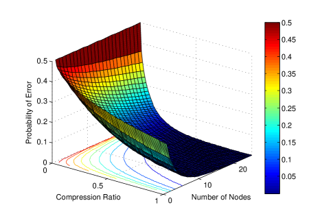
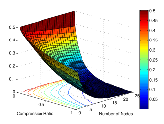
Figure 2: Prob. of error as a function of number of nodes and compression ratio c=M/P𝑐𝑀𝑃c=M/P for SNR=3dB𝑆𝑁𝑅3𝑑𝐵SNR=3dB

To corroborate our theoretical results, in Figure 2 we present the behavior of PEsubscript𝑃𝐸P_{E} with respect of collaboration and compression. We plot PEsubscript𝑃𝐸P_{E} as a function of the number of nodes N𝑁N and compression ratio c𝑐c. We assume that SNR=3dB𝑆𝑁𝑅3𝑑𝐵SNR=3dB. It can be seen from Figure 2 that PEsubscript𝑃𝐸P_{E} is a monotonically decreasing function of c𝑐c and N𝑁N, and, therefore, the performance loss due to compression can be compensated by exploiting spatial diversity or collaboration.

In order to more clearly illustrate the behavior of PEsubscript𝑃𝐸P_{E} with respect to compression and collaboration, we also establish the following corollary of Theorem 1 using the Chernoff Bound.

Corollary 1.

Suppose that PMP^𝑃𝑀^𝑃\sqrt{\frac{P}{M}}\hat{P} provides an ϵitalic-ϵ\epsilon-stable embedding of (𝒮,{0})𝒮0(\mathcal{S},\{0\}). Then for any deterministic signal sS𝑠𝑆s\in S, we have

PE12exp(18cNs22β1).subscript𝑃𝐸1218𝑐𝑁superscriptsubscriptnorm𝑠22superscript𝛽1P_{E}\leq\frac{1}{2}\exp\left(-\frac{1}{8}cN\frac{\|s\|_{2}^{2}}{\beta^{-1}}\right).

Corollary 1 suggests that the error probability vanishes exponentially fast as we increase either the compression ratio c𝑐c or the number of collaborating nodes N𝑁N.

Next, we extend the above analysis to the case where the signal of interest is a random signal such that s𝒩(μ,α1IP)similar-to𝑠𝒩𝜇superscript𝛼1subscript𝐼𝑃s\sim\mathcal{N}(\mu,\alpha^{-1}I_{P}).

III-B Random Signal with Arbitrary Mean Case

Let the signal of interest be s𝒩(μ,α1IP)similar-to𝑠𝒩𝜇superscript𝛼1subscript𝐼𝑃s\sim\mathcal{N}(\mu,\alpha^{-1}I_{P}) with an arbitrary μ𝜇\mu. Then, the collaborative compressive detector is given by

α1β1i=1NyiT(ϕϕT)1yi+2i=1NyiT(ϕϕT)1μH1H0λsuperscript𝛼1superscript𝛽1superscriptsubscript𝑖1𝑁superscriptsubscript𝑦𝑖𝑇superscriptitalic-ϕsuperscriptitalic-ϕ𝑇1subscript𝑦𝑖2superscriptsubscript𝑖1𝑁superscriptsubscript𝑦𝑖𝑇superscriptitalic-ϕsuperscriptitalic-ϕ𝑇1𝜇subscriptsuperscriptgreater-than-or-less-thansubscript𝐻1subscript𝐻0𝜆\frac{\alpha^{-1}}{\beta^{-1}}\sum\limits_{i=1}^{N}y_{i}^{T}(\phi\phi^{T})^{-1}y_{i}+2\sum\limits_{i=1}^{N}y_{i}^{T}(\phi\phi^{T})^{-1}\mu\quad\mathop{\stackrel{{\scriptstyle H_{1}}}{{\gtrless}}}_{H_{0}}\quad\lambda

where λ=(α1+β1)[NMlog(1+α1β1)]+N(ϕμ)T(ϕϕT)1ϕμ𝜆superscript𝛼1superscript𝛽1delimited-[]𝑁𝑀1superscript𝛼1superscript𝛽1𝑁superscriptitalic-ϕ𝜇𝑇superscriptitalic-ϕsuperscriptitalic-ϕ𝑇1italic-ϕ𝜇\lambda=(\alpha^{-1}+\beta^{-1})\left[NM\log\left(1+\frac{\alpha^{-1}}{\beta^{-1}}\right)\right]+N(\phi\mu)^{T}(\phi\phi^{T})^{-1}\phi\mu. Note that, the test statistic is of the form i=1N[yiTAyi+2bTyi]superscriptsubscript𝑖1𝑁delimited-[]superscriptsubscript𝑦𝑖𝑇𝐴subscript𝑦𝑖2superscript𝑏𝑇subscript𝑦𝑖\sum\limits_{i=1}^{N}\left[y_{i}^{T}Ay_{i}+2b^{T}y_{i}\right] with A=α1β1(ϕϕT)1𝐴superscript𝛼1superscript𝛽1superscriptitalic-ϕsuperscriptitalic-ϕ𝑇1A=\frac{\alpha^{-1}}{\beta^{-1}}(\phi\phi^{T})^{-1} and b=(ϕϕT)1ϕμ𝑏superscriptitalic-ϕsuperscriptitalic-ϕ𝑇1italic-ϕ𝜇b=(\phi\phi^{T})^{-1}\phi\mu. In general, it is difficult to find the PDF of such an expression in a closed form. Next, we state a Lemma from [25], which will be used to derive the distribution of the test statistic in a closed form.

Lemma 1 ([25]).

Let A𝐴A be a symmetric matrix and x𝒩(μ,V)similar-to𝑥𝒩𝜇𝑉x\sim\mathcal{N}(\mu,V), where V𝑉V is positive definite (hence nonsingular). The necessary and sufficient condition that xTAx+2bTx+csuperscript𝑥𝑇𝐴𝑥2superscript𝑏𝑇𝑥𝑐x^{T}Ax+2b^{T}x+c follows a noncentral chi-squared distribution 𝒳k2(δ)subscriptsuperscript𝒳2𝑘𝛿\mathcal{X}^{2}_{k}(\delta) with k𝑘k degrees of freedom and noncentrality parameter δ𝛿\delta is that

[A1bT]V[A:b]=[AbbTc]\begin{bmatrix}A\\ {1}\\ b^{T}\end{bmatrix}V[A:b]=\begin{bmatrix}A&b\\ b^{T}&c\end{bmatrix} (10)

in which case k𝑘k is the rank of A𝐴A and δ=μTAμ+2bTμ+c𝛿superscript𝜇𝑇𝐴𝜇2superscript𝑏𝑇𝜇𝑐\delta=\mu^{T}A\mu+2b^{T}\mu+c.

Next, using Lemma 1 we state the following proposition.

Proposition 1.

For a P×P𝑃𝑃P\times P symmetric and idempotent matrix S𝑆S and ui𝒩(μ,σ2IP)similar-tosubscript𝑢𝑖𝒩𝜇superscript𝜎2subscript𝐼𝑃u_{i}\sim\mathcal{N}(\mu,\sigma^{2}I_{P}), the test statistic of the form uiTAui+2bTui+csuperscriptsubscript𝑢𝑖𝑇𝐴subscript𝑢𝑖2superscript𝑏𝑇subscript𝑢𝑖𝑐u_{i}^{T}Au_{i}+2b^{T}u_{i}+c with A=1σ2S𝐴1superscript𝜎2𝑆A=\frac{1}{\sigma^{2}}S, bT=1σ2zTSsuperscript𝑏𝑇1superscript𝜎2superscript𝑧𝑇𝑆b^{T}=\frac{1}{\sigma^{2}}z^{T}S and c=1σ2zTSz𝑐1superscript𝜎2superscript𝑧𝑇𝑆𝑧c=\frac{1}{\sigma^{2}}z^{T}Sz follows a noncentral chi-squared distribution 𝒳k2(δ)subscriptsuperscript𝒳2𝑘𝛿\mathcal{X}^{2}_{k}(\delta) where k=Rank(S)𝑘Rank𝑆k=\text{Rank}(S) and δ=1σ2(μTSμ+2zTSμ+zTSz)𝛿1superscript𝜎2superscript𝜇𝑇𝑆𝜇2superscript𝑧𝑇𝑆𝜇superscript𝑧𝑇𝑆𝑧\delta=\frac{1}{\sigma^{2}}\left(\mu^{T}S\mu+2z^{T}S\mu+z^{T}Sz\right) for any arbitrary P×1𝑃1P\times 1 vector z𝑧z.

Proof.

To prove the proposition, it is sufficient to show that the above mentioned A𝐴A, b𝑏b and c𝑐c satisfy condition (10) in Lemma 1 for any arbitrary P×1𝑃1P\times 1 vector z𝑧z. Notice that, S𝑆S satisfies the following properties: symmetric ST=Ssuperscript𝑆𝑇𝑆S^{T}=S and idempotent S2=Ssuperscript𝑆2𝑆S^{2}=S. Thus,

[A1bT]V[A:b]\displaystyle\begin{bmatrix}A\\ {1}\\ b^{T}\end{bmatrix}V[A:b] =\displaystyle= [1σ2S11σ2zTS][σ2IP][1σ2S1σ2Sz]matrix1superscript𝜎2𝑆11superscript𝜎2superscript𝑧𝑇𝑆delimited-[]superscript𝜎2subscript𝐼𝑃delimited-[]1superscript𝜎2𝑆1superscript𝜎2𝑆𝑧\displaystyle\begin{bmatrix}\frac{1}{\sigma^{2}}S\\ {1}\\ \frac{1}{\sigma^{2}}z^{T}S\end{bmatrix}\left[\sigma^{2}I_{P}\right]\left[\frac{1}{\sigma^{2}}S\;\vdots\;\frac{1}{\sigma^{2}}Sz\right]
=\displaystyle= [P^1zTS][1σ2S1σ2Sz]matrix^𝑃1superscript𝑧𝑇𝑆delimited-[]1superscript𝜎2𝑆1superscript𝜎2𝑆𝑧\displaystyle\begin{bmatrix}\hat{P}\\ {1}\\ z^{T}S\end{bmatrix}\left[\frac{1}{\sigma^{2}}S\;\vdots\;\frac{1}{\sigma^{2}}Sz\right]
=\displaystyle= [1σ2SS1σ2SSz1σ2zTSS1σ2zTSSz]matrix1superscript𝜎2𝑆𝑆1superscript𝜎2𝑆𝑆𝑧1superscript𝜎2superscript𝑧𝑇𝑆𝑆1superscript𝜎2superscript𝑧𝑇𝑆𝑆𝑧\displaystyle\begin{bmatrix}\frac{1}{\sigma^{2}}SS&\frac{1}{\sigma^{2}}SSz\\ \frac{1}{\sigma^{2}}z^{T}SS&\frac{1}{\sigma^{2}}z^{T}SSz\end{bmatrix}
=\displaystyle= [AbbTc]matrix𝐴𝑏superscript𝑏𝑇𝑐\displaystyle\begin{bmatrix}A&b\\ b^{T}&c\end{bmatrix}

Thus, the test statistic follows a noncentral chi-squared distribution 𝒳k2(δ)subscriptsuperscript𝒳2𝑘𝛿\mathcal{X}^{2}_{k}(\delta) where k=Rank(S)𝑘Rank𝑆k=\text{Rank}(S) and δ=1σ2(μTSμ+2zTSμ+zTSz)𝛿1superscript𝜎2superscript𝜇𝑇𝑆𝜇2superscript𝑧𝑇𝑆𝜇superscript𝑧𝑇𝑆𝑧\delta=\frac{1}{\sigma^{2}}\left(\mu^{T}S\mu+2z^{T}S\mu+z^{T}Sz\right) for any arbitrary z𝑧z. ∎

Using these results, the collaborative compressive detector reduces to:

α1β1i=1NyiT(ϕϕT)1yi+2i=1NyiT(ϕϕT)1μH1H0λ.superscript𝛼1superscript𝛽1superscriptsubscript𝑖1𝑁superscriptsubscript𝑦𝑖𝑇superscriptitalic-ϕsuperscriptitalic-ϕ𝑇1subscript𝑦𝑖2superscriptsubscript𝑖1𝑁superscriptsubscript𝑦𝑖𝑇superscriptitalic-ϕsuperscriptitalic-ϕ𝑇1𝜇subscriptsuperscriptgreater-than-or-less-thansubscript𝐻1subscript𝐻0𝜆\frac{\alpha^{-1}}{\beta^{-1}}\sum\limits_{i=1}^{N}y_{i}^{T}(\phi\phi^{T})^{-1}y_{i}+2\sum\limits_{i=1}^{N}y_{i}^{T}(\phi\phi^{T})^{-1}\mu\quad\mathop{\stackrel{{\scriptstyle H_{1}}}{{\gtrless}}}_{H_{0}}\quad\lambda.

Using the fact that yi=ϕuisubscript𝑦𝑖italic-ϕsubscript𝑢𝑖y_{i}=\phi u_{i} and rearranging the terms, we get

i=1N[uiTP^ui+2β1α1μTP^ui+(β1α1)2μTP^μ]H1H0τsuperscriptsubscript𝑖1𝑁delimited-[]superscriptsubscript𝑢𝑖𝑇^𝑃subscript𝑢𝑖2superscript𝛽1superscript𝛼1superscript𝜇𝑇^𝑃subscript𝑢𝑖superscriptsuperscript𝛽1superscript𝛼12superscript𝜇𝑇^𝑃𝜇subscriptsuperscriptgreater-than-or-less-thansubscript𝐻1subscript𝐻0𝜏\sum\limits_{i=1}^{N}\left[u_{i}^{T}\hat{P}u_{i}+2\frac{\beta^{-1}}{\alpha^{-1}}\mu^{T}\hat{P}u_{i}+\left(\frac{\beta^{-1}}{\alpha^{-1}}\right)^{2}\mu^{T}\hat{P}\mu\right]\quad\mathop{\stackrel{{\scriptstyle H_{1}}}{{\gtrless}}}_{H_{0}}\quad\tau

where P^=ϕT(ϕϕT)1ϕ^𝑃superscriptitalic-ϕ𝑇superscriptitalic-ϕsuperscriptitalic-ϕ𝑇1italic-ϕ\hat{P}=\phi^{T}(\phi\phi^{T})^{-1}\phi and τ=β1α1λ+N(β1α1)2μTP^μ𝜏superscript𝛽1superscript𝛼1𝜆𝑁superscriptsuperscript𝛽1superscript𝛼12superscript𝜇𝑇^𝑃𝜇\tau=\frac{\beta^{-1}}{\alpha^{-1}}\lambda+N\left(\frac{\beta^{-1}}{\alpha^{-1}}\right)^{2}\mu^{T}\hat{P}\mu. Note that, the FC does not have access to uisubscript𝑢𝑖u_{i} and the above test statistic is used only for deriving the PDF of the original test statistic.
Refer to caption
Refer to caption
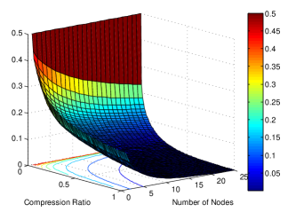
Figure 3: Prob of error (Pesubscript𝑃𝑒P_{e}) analysis when (α1,β1)=(1,20)superscript𝛼1superscript𝛽1120(\alpha^{-1},\beta^{-1})=(1,20) and P=100𝑃100P=100. 3 Pesubscript𝑃𝑒P_{e} with varying ((c,N)𝑐𝑁(c,\;N)) when μ=0𝜇0\mu=0. 3 Pesubscript𝑃𝑒P_{e} with varying ((c,N)𝑐𝑁(c,\;N)) when μ=103𝜇superscript103\mu=10^{-3}.
Theorem 2.

For a projection matrix P^=ϕT(ϕϕT)1ϕ^𝑃superscriptitalic-ϕ𝑇superscriptitalic-ϕsuperscriptitalic-ϕ𝑇1italic-ϕ\hat{P}=\phi^{T}(\phi\phi^{T})^{-1}\phi and ui𝒩(μ,σk2IP)similar-tosubscript𝑢𝑖𝒩𝜇superscriptsubscript𝜎𝑘2subscript𝐼𝑃u_{i}\sim\mathcal{N}(\mu,\sigma_{k}^{2}I_{P}) under the hypothesis Hksubscript𝐻𝑘H_{k}, the test statistic

Λ(𝐲)=i=1N[uiTP^ui+2β1α1μTP^ui+(β1α1)2μTP^μ]Λ𝐲superscriptsubscript𝑖1𝑁delimited-[]superscriptsubscript𝑢𝑖𝑇^𝑃subscript𝑢𝑖2superscript𝛽1superscript𝛼1superscript𝜇𝑇^𝑃subscript𝑢𝑖superscriptsuperscript𝛽1superscript𝛼12superscript𝜇𝑇^𝑃𝜇\Lambda(\mathbf{y})=\sum\limits_{i=1}^{N}\left[u_{i}^{T}\hat{P}u_{i}+2\frac{\beta^{-1}}{\alpha^{-1}}\mu^{T}\hat{P}u_{i}+\left(\frac{\beta^{-1}}{\alpha^{-1}}\right)^{2}\mu^{T}\hat{P}\mu\right]

has the following distribution

Λ(𝐲)σk2{𝒳NM2(δ0),underH0𝒳NM2(Nδ1)underH1similar-toΛ𝐲superscriptsubscript𝜎𝑘2casessubscriptsuperscript𝒳2𝑁𝑀subscript𝛿0undersubscript𝐻0missing-subexpressionsubscriptsuperscript𝒳2𝑁𝑀𝑁subscript𝛿1undersubscript𝐻1missing-subexpression\frac{\Lambda(\mathbf{y})}{\sigma_{k}^{2}}\sim\left\{\begin{array}[]{rll}\mathcal{X}^{2}_{NM}(\delta_{0}),&\mbox{under}\ H_{0}\\ \mathcal{X}^{2}_{NM}(N\delta_{1})&\mbox{under}\ H_{1}\end{array}\right.

where σ02=β1superscriptsubscript𝜎02superscript𝛽1\sigma_{0}^{2}=\beta^{-1}, σ12=α1+β1superscriptsubscript𝜎12superscript𝛼1superscript𝛽1\sigma_{1}^{2}=\alpha^{-1}+\beta^{-1} and 𝒳NM2(δk)subscriptsuperscript𝒳2𝑁𝑀subscript𝛿𝑘\mathcal{X}^{2}_{NM}(\delta_{k}) denotes noncentral chi-square distribution with NM𝑁𝑀NM degrees of freedom and parameters δ0=0subscript𝛿00\delta_{0}=0 and δ1=P^μ22α1(1+β1α1)subscript𝛿1superscriptsubscriptnorm^𝑃𝜇22superscript𝛼11superscript𝛽1superscript𝛼1\delta_{1}=\frac{||\hat{P}\mu||_{2}^{2}}{\alpha^{-1}}\left(1+\frac{\beta^{-1}}{\alpha^{-1}}\right).

Proof.

Let us denote the test static by Λ(𝐲)=i=1NΛ(yi)Λ𝐲superscriptsubscript𝑖1𝑁Λsubscript𝑦𝑖\Lambda(\mathbf{y})=\sum\limits_{i=1}^{N}\Lambda({y_{i}}) with

Λ(yi)=[uiTP^ui+2β1α1μTP^ui+(β1α1)2μTP^μ].Λsubscript𝑦𝑖delimited-[]superscriptsubscript𝑢𝑖𝑇^𝑃subscript𝑢𝑖2superscript𝛽1superscript𝛼1superscript𝜇𝑇^𝑃subscript𝑢𝑖superscriptsuperscript𝛽1superscript𝛼12superscript𝜇𝑇^𝑃𝜇\Lambda({y_{i}})=\left[u_{i}^{T}\hat{P}u_{i}+2\frac{\beta^{-1}}{\alpha^{-1}}\mu^{T}\hat{P}u_{i}+\left(\frac{\beta^{-1}}{\alpha^{-1}}\right)^{2}\mu^{T}\hat{P}\mu\right].

Now notice that, Λ(yi)σk2Λsubscript𝑦𝑖superscriptsubscript𝜎𝑘2\frac{\Lambda({y_{i}})}{\sigma_{k}^{2}} is of the form uiTAui+2bTui+csuperscriptsubscript𝑢𝑖𝑇𝐴subscript𝑢𝑖2superscript𝑏𝑇subscript𝑢𝑖𝑐u_{i}^{T}Au_{i}+2b^{T}u_{i}+c with A=P^σk2𝐴^𝑃superscriptsubscript𝜎𝑘2A=\frac{\hat{P}}{\sigma_{k}^{2}}, bT=zTP^σk2superscript𝑏𝑇superscript𝑧𝑇^𝑃superscriptsubscript𝜎𝑘2b^{T}=\frac{z^{T}\hat{P}}{\sigma_{k}^{2}}, z=β1α1μ𝑧superscript𝛽1superscript𝛼1𝜇z=\frac{\beta^{-1}}{\alpha^{-1}}\mu and c=zTP^zσk2𝑐superscript𝑧𝑇^𝑃𝑧superscriptsubscript𝜎𝑘2c=\frac{z^{T}\hat{P}z}{\sigma_{k}^{2}}. Also note that, the projection matrix P^=ϕT(ϕϕT)1ϕ^𝑃superscriptitalic-ϕ𝑇superscriptitalic-ϕsuperscriptitalic-ϕ𝑇1italic-ϕ\hat{P}=\phi^{T}(\phi\phi^{T})^{-1}\phi is both symmetric and idempotent with rank(P^)=M^𝑃𝑀(\hat{P})=M. As a result, using Proposition 1 and the fact that Λ(𝐲)σk2Λ𝐲superscriptsubscript𝜎𝑘2\frac{\Lambda(\mathbf{y})}{\sigma_{k}^{2}} is the sum of N𝑁N I.I.D. chi-squared random variables Λ(yi)σk2Λsubscript𝑦𝑖superscriptsubscript𝜎𝑘2\frac{\Lambda(y_{i})}{\sigma_{k}^{2}}, the result in the Theorem 2 can be derived. ∎

If NM𝑁𝑀NM is large enough, then, the following approximations hold

Λ(𝐲)σk2{𝒩(NM,2NM),underH0𝒩((NM+Nδ1),2(NM+Nδ1)underH1\frac{\Lambda(\mathbf{y})}{\sigma_{k}^{2}}\sim\left\{\begin{array}[]{rll}\mathcal{N}(NM,2NM),&\mbox{under}\ H_{0}\\ \mathcal{N}((NM+N\delta_{1}),2(NM+N\delta_{1})&\mbox{under}\ H_{1}\end{array}\right.

where δ1=P^μ22α1(1+β1α1)subscript𝛿1superscriptsubscriptnorm^𝑃𝜇22superscript𝛼11superscript𝛽1superscript𝛼1\delta_{1}=\frac{||\hat{P}\mu||_{2}^{2}}{\alpha^{-1}}\left(1+\frac{\beta^{-1}}{\alpha^{-1}}\right). As a result, we have

PF=P(Λ(𝐲)β1>τβ1|H0)=Q(τβ1NM2NM)subscript𝑃𝐹𝑃Λ𝐲superscript𝛽1conditional𝜏superscript𝛽1subscript𝐻0𝑄𝜏superscript𝛽1𝑁𝑀2𝑁𝑀\qquad P_{F}=P\left(\frac{\Lambda(\mathbf{y})}{\beta^{-1}}>\frac{\tau}{\beta^{-1}}|H_{0}\right)=Q\left(\frac{\frac{\tau}{\beta^{-1}}-NM}{\sqrt{2NM}}\right)

and

PDsubscript𝑃𝐷\displaystyle P_{D} =\displaystyle= P(Λ(𝐲)α1+β1>τα1+β1|H1)𝑃Λ𝐲superscript𝛼1superscript𝛽1conditional𝜏superscript𝛼1superscript𝛽1subscript𝐻1\displaystyle P\left(\frac{\Lambda(\mathbf{y})}{\alpha^{-1}+\beta^{-1}}>\frac{\tau}{\alpha^{-1}+\beta^{-1}}|H_{1}\right)
=\displaystyle= Q(τα1+β1NMNδ12(NM+Nδ1))𝑄𝜏superscript𝛼1superscript𝛽1𝑁𝑀𝑁subscript𝛿12𝑁𝑀𝑁subscript𝛿1\displaystyle Q\left(\frac{\frac{\tau}{\alpha^{-1}+\beta^{-1}}-NM-N\delta_{1}}{\sqrt{2(NM+N\delta_{1})}}\right)

where τ=β1α1λ+N(β1α1)2P^μ22𝜏superscript𝛽1superscript𝛼1𝜆𝑁superscriptsuperscript𝛽1superscript𝛼12superscriptsubscriptnorm^𝑃𝜇22\tau=\frac{\beta^{-1}}{\alpha^{-1}}\lambda+N\left(\frac{\beta^{-1}}{\alpha^{-1}}\right)^{2}||\hat{P}\mu||_{2}^{2}, λ=(α1+β1)[NMlog(1+α1β1)]+NP^μ22𝜆superscript𝛼1superscript𝛽1delimited-[]𝑁𝑀1superscript𝛼1superscript𝛽1𝑁superscriptsubscriptnorm^𝑃𝜇22\lambda=(\alpha^{-1}+\beta^{-1})\left[NM\log\left(1+\frac{\alpha^{-1}}{\beta^{-1}}\right)\right]+N||\hat{P}\mu||_{2}^{2} and δ1=P^μ22α1(1+β1α1)subscript𝛿1superscriptsubscriptnorm^𝑃𝜇22superscript𝛼11superscript𝛽1superscript𝛼1\delta_{1}=\frac{||\hat{P}\mu||_{2}^{2}}{\alpha^{-1}}\left(1+\frac{\beta^{-1}}{\alpha^{-1}}\right).

The detection performance of the system is a function of the projection operator P^^𝑃\hat{P}. Next, we provide approximations to the performance of the collaborative compressive detector using the concept of ϵitalic-ϵ\epsilon-stable embedding of the mean μ𝜇\mu.

Theorem 3.

Suppose that PMP^𝑃𝑀^𝑃\sqrt{\frac{P}{M}}\hat{P} provides an ϵitalic-ϵ\epsilon-stable embedding of (𝒰,{0})𝒰0(\mathcal{U},\{0\}). Then for any random signal s𝒩(μ,α1IP)similar-to𝑠𝒩𝜇superscript𝛼1subscript𝐼𝑃s\sim\mathcal{N}(\mu,\alpha^{-1}I_{P}) with μ𝒰𝜇𝒰\mu\in\mathcal{U}, the probability of error of the collaborative compressive detector can be approximated as

PE=12Q(cNτ0)+12(Q(cNτ1))subscript𝑃𝐸12𝑄𝑐𝑁subscript𝜏012𝑄𝑐𝑁subscript𝜏1P_{E}=\dfrac{1}{2}Q\left(\sqrt{cN}\tau_{0}\right)+\dfrac{1}{2}\left(Q\left(\sqrt{cN}\tau_{1}\right)\right)

where τ0=P2((1+τ1)(log(1+τ)+μ22α1P)1)subscript𝜏0𝑃21superscript𝜏11𝜏superscriptsubscriptnorm𝜇22superscript𝛼1𝑃1\tau_{0}=\sqrt{\frac{P}{2}}\left(\left(1+\tau^{-1}\right)\left(\log\left(1+\tau\right)+\frac{\|\mu\|_{2}^{2}}{\alpha^{-1}P}\right)-1\right), τ1=P+δ12(1τ1(Plog(1+τ)+μ22α1)P+δ1)subscript𝜏1𝑃superscriptsubscript𝛿121superscript𝜏1𝑃1𝜏superscriptsubscriptnorm𝜇22superscript𝛼1𝑃superscriptsubscript𝛿1\tau_{1}=\sqrt{\frac{P+\delta_{1}^{\prime}}{2}}\left(1-\frac{\tau^{-1}\left(P\log(1+\tau)+\frac{\|\mu\|_{2}^{2}}{\alpha^{-1}}\right)}{P+\delta_{1}^{\prime}}\right) with δ1=μ22α1(1+τ1)superscriptsubscript𝛿1superscriptsubscriptnorm𝜇22superscript𝛼11superscript𝜏1\delta_{1}^{\prime}=\frac{\|\mu\|_{2}^{2}}{\alpha^{-1}}(1+\tau^{-1}) and τ=α1β1𝜏superscript𝛼1superscript𝛽1\tau=\frac{\alpha^{-1}}{\beta^{-1}}.

Proof.

By our assumption that PMP^𝑃𝑀^𝑃\sqrt{\frac{P}{M}}\hat{P} provides an ϵitalic-ϵ\epsilon-stable embedding of (𝒰,{0})𝒰0(\mathcal{U},\{0\}), we know that

1ϵμ2PMP^μ21+ϵμ2.1italic-ϵsubscriptnorm𝜇2𝑃𝑀subscriptnorm^𝑃𝜇21italic-ϵsubscriptnorm𝜇2\sqrt{1-\epsilon}\;\|\mu\|_{2}\leq\sqrt{\frac{P}{M}}\;\|\hat{P}\mu\|_{2}\leq\sqrt{1+\epsilon}\;\|\mu\|_{2}. (11)

In other words, for large values of NM𝑁𝑀NM the following approximation holds: |P^μ22MPμ22=cμ22superscriptsubscriptdelimited-|‖^𝑃𝜇22𝑀𝑃superscriptsubscriptnorm𝜇22𝑐superscriptsubscriptnorm𝜇22|\hat{P}\mu\|_{2}^{2}\approx\frac{M}{P}\|\mu\|_{2}^{2}=c\|\mu\|_{2}^{2}. The proof follows from the fact that Q(x)=1Q(x)𝑄𝑥1𝑄𝑥Q(x)=1-Q(-x) and by plugging in

PF=Q(cNτ0)subscript𝑃𝐹𝑄𝑐𝑁subscript𝜏0P_{F}=Q\left(\sqrt{cN}\tau_{0}\right) (12)

and

PD=Q(cNτ1)subscript𝑃𝐷𝑄𝑐𝑁subscript𝜏1P_{D}=Q\left(-\sqrt{cN}\tau_{1}\right) (13)

in the equation PE=12PF+12(1PD)subscript𝑃𝐸12subscript𝑃𝐹121subscript𝑃𝐷P_{E}=\dfrac{1}{2}P_{F}+\dfrac{1}{2}(1-P_{D}), the above results can be derived. ∎

Note that, (τ1)τ0subscript𝜏1subscript𝜏0(-\tau_{1})\leq\tau_{0} and, therefore, PDPFsubscript𝑃𝐷subscript𝑃𝐹P_{D}\geq P_{F}. Similar to the deterministic signal case, if Nc1𝑁superscript𝑐1N\geq c^{-1} the loss due to compression with a single node can be recovered in collaborative compressive detection for the random signal case as well. For a fixed M𝑀M, as the number of collaborating nodes approaches infinity, i.e., N𝑁N\rightarrow\infty, the probability of error vanishes. We would like to point out that by plugging in μ=0𝜇0\mu=0 in the above expressions, results for the zero mean signal case can be derived (which are consistent with [6, 9]).

To gain insights into Theorem 3, we present illustrative examples that corroborate our results. In Figure 3 we plot the probability of error PEsubscript𝑃𝐸P_{E} as a function of the number of nodes N𝑁N and compression ratio c𝑐c. We assume that the signal of interest is s𝒩(0,IP)similar-to𝑠𝒩0subscript𝐼𝑃s\sim\mathcal{N}(0,I_{P}) and noise vi𝒩(0,20IP)similar-tosubscript𝑣𝑖𝒩020subscript𝐼𝑃v_{i}\sim\mathcal{N}(0,20I_{P}), with original length of the signal being P=100𝑃100P=100. It can be seen from the figure that PEsubscript𝑃𝐸P_{E} is a monotonically decreasing function of (c,N)𝑐𝑁(c,N). In Figure 3, we plot the probability of error PEsubscript𝑃𝐸P_{E} as a function of (c,N)𝑐𝑁(c,N) when the signal of interest is s𝒩(μ,IP)similar-to𝑠𝒩𝜇subscript𝐼𝑃s\sim\mathcal{N}(\mu,I_{P}) with μ22=103superscriptsubscriptnorm𝜇22superscript103\|\mu\|_{2}^{2}=10^{-3}. Similar to Figure 3, PEsubscript𝑃𝐸P_{E} decreases monotonically with (c,N)𝑐𝑁(c,N), however, with a much faster rate. In order to more clearly illustrate this behavior of PEsubscript𝑃𝐸P_{E}, we also establish the following corollary of Theorem 3.

Corollary 2.

Suppose that PMP^𝑃𝑀^𝑃\sqrt{\frac{P}{M}}\hat{P} provides an ϵitalic-ϵ\epsilon-stable embedding of (𝒰,{0})𝒰0(\mathcal{U},\{0\}). Then for any random signal s𝒩(μ,α1IP)similar-to𝑠𝒩𝜇superscript𝛼1subscript𝐼𝑃s\sim\mathcal{N}(\mu,\alpha^{-1}I_{P}) with μ𝒰𝜇𝒰\mu\in\mathcal{U}, the error probability PEsubscript𝑃𝐸P_{E} of the collaborative compressive detector satisfies

PE14exp(cN2τ02)+14exp(cN2τ12).subscript𝑃𝐸14𝑐𝑁2superscriptsubscript𝜏0214𝑐𝑁2superscriptsubscript𝜏12P_{E}\leq\frac{1}{4}\exp\left(-\frac{cN}{2}\tau_{0}^{2}\right)+\frac{1}{4}\exp\left(-\frac{cN}{2}\tau_{1}^{2}\right).
Proof.

To prove the corollary, we first show that both τ0subscript𝜏0\tau_{0} and τ1subscript𝜏1\tau_{1} as given in Theorem 3 are positive. Let us denote by τk(μ=0)subscript𝜏𝑘𝜇0\tau_{k}(\mu=0) the expression when μ=0𝜇0\mu=0 is plugged in the expression for τksubscript𝜏𝑘\tau_{k} for k{0,1}𝑘01k\in\{0,1\}. Then, it can be shown that τkτk(μ=0)subscript𝜏𝑘subscript𝜏𝑘𝜇0\tau_{k}\geq\tau_{k}(\mu=0) for k{0,1}𝑘01k\in\{0,1\}. Now, a sufficient condition for τk>0subscript𝜏𝑘0\tau_{k}>0 is τk(μ=0)>0subscript𝜏𝑘𝜇00\tau_{k}(\mu=0)>0 for k{0,1}𝑘01k\in\{0,1\}. The condition for τ0(μ=0)>0subscript𝜏0𝜇00\tau_{0}(\mu=0)>0 and τ1(μ=0)>0subscript𝜏1𝜇00\tau_{1}(\mu=0)>0 to be true can be written as

11+β1α1<log(1+α1β1)<α1β1.11superscript𝛽1superscript𝛼11superscript𝛼1superscript𝛽1superscript𝛼1superscript𝛽1\frac{1}{1+\frac{\beta^{-1}}{\alpha^{-1}}}<\log\left(1+\frac{\alpha^{-1}}{\beta^{-1}}\right)<\frac{\alpha^{-1}}{\beta^{-1}}.

The above condition can be shown to be true by applying the logarithm inequality τ1+τ<log(1+τ)<τ𝜏1𝜏1𝜏𝜏\frac{\tau}{1+\tau}<\log(1+\tau)<\tau with τ=α1β1𝜏superscript𝛼1superscript𝛽1\tau=\frac{\alpha^{-1}}{\beta^{-1}}. Now using the Chernoff bound (i.e., Q(x)12exp(x22)𝑄𝑥12superscript𝑥22Q(x)\leq\frac{1}{2}\exp(-\frac{x^{2}}{2}) for x>0𝑥0x>0), it can be shown that

PE14exp(cN2τ02)+14exp(cN2τ12).subscript𝑃𝐸14𝑐𝑁2superscriptsubscript𝜏0214𝑐𝑁2superscriptsubscript𝜏12P_{E}\leq\frac{1}{4}\exp\left(-\frac{cN}{2}\tau_{0}^{2}\right)+\frac{1}{4}\exp\left(-\frac{cN}{2}\tau_{1}^{2}\right).

The above expression suggests that PEsubscript𝑃𝐸P_{E} vanishes exponentially fast as we increase either the compression ratio c𝑐c or the number of collaborating nodes N𝑁N. ∎

Next, we consider the problem where the network operates in the presence of an eavesdropper who wants to discover the state of the nature being monitored by the system. The FC’s goal is to implement the appropriate countermeasures to keep the data regarding the presence of the phenomenon secret from the eavesdropper.

IV Collaborative Compressive Detection in the Presence of an Eavesdropper

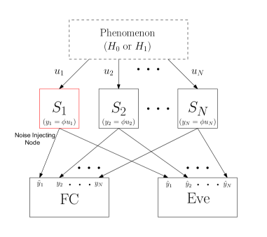
In a collaborative compressive detection framework, the FC receives compressed observation vectors, 𝐲=[y1,,yN]𝐲subscript𝑦1subscript𝑦𝑁\mathbf{y}=[y_{1},\cdots,y_{N}], from the nodes and makes the global decision about the presence of the random signal vector222In rest of the paper, we will consider only the random signal detection case. Deterministic signal can be seen as a special case of random signal s𝑠s with variance α1=0superscript𝛼10\alpha^{-1}=0 and results for the deterministic signal case can be obtained by plugging in α1=0superscript𝛼10\alpha^{-1}=0 in corresponding expressions for the random signal case. s𝒩(μ,α1IP)similar-to𝑠𝒩𝜇superscript𝛼1subscript𝐼𝑃s\sim\mathcal{N}(\mu,\alpha^{-1}I_{P}) with μ0𝜇0\mu\neq 0. The transmission of the nodes, however, may be observed by an eavesdropper who also wants to discover the state of the phenomenon (see Figure 4). To keep the data regarding the presence of the phenomenon secret from the eavesdropper, we propose to use cooperating trustworthy nodes that assist the FC by injecting artificial noise to mislead the eavesdroppers to improve the security performance of the system.
Refer to caption
Figure 4: Collaborative Compressive Detection Network in the Presence of an Eavesdropper

IV-A Artificial Noise Injection Model

It is assumed that B𝐵B out of N𝑁N nodes (or α𝛼\alpha fraction of the nodes) inject artificial noise according to the model given next. Nodes tamper their data yisubscript𝑦𝑖y_{i} and send yi~~subscript𝑦𝑖\tilde{y_{i}} in the following manner:

Under H0subscript𝐻0H_{0}:

yi~={ϕ(vi+Wi)with probabilityP10ϕ(viWi)with probabilityP20ϕviwith probability(1P10P20)~subscript𝑦𝑖casesitalic-ϕsubscript𝑣𝑖subscript𝑊𝑖with probabilitysuperscriptsubscript𝑃10missing-subexpressionitalic-ϕsubscript𝑣𝑖subscript𝑊𝑖with probabilitysuperscriptsubscript𝑃20missing-subexpressionitalic-ϕsubscript𝑣𝑖with probability1superscriptsubscript𝑃10superscriptsubscript𝑃20missing-subexpression\tilde{y_{i}}=\left\{\begin{array}[]{rll}\phi(v_{i}+W_{i})&\mbox{with probability}\ P_{1}^{0}\\ \phi(v_{i}-W_{i})&\mbox{with probability}\ P_{2}^{0}\\ \phi v_{i}&\mbox{with probability}\ (1-P_{1}^{0}-P_{2}^{0})\\ \end{array}\right.

Under H1subscript𝐻1H_{1}:

yi~={ϕ(s+vi+Wi)with probabilityP11ϕ(s+viWi)with probabilityP21ϕ(s+vi)with probability(1P11P21)~subscript𝑦𝑖casesitalic-ϕ𝑠subscript𝑣𝑖subscript𝑊𝑖with probabilitysuperscriptsubscript𝑃11missing-subexpressionitalic-ϕ𝑠subscript𝑣𝑖subscript𝑊𝑖with probabilitysuperscriptsubscript𝑃21missing-subexpressionitalic-ϕ𝑠subscript𝑣𝑖with probability1superscriptsubscript𝑃11superscriptsubscript𝑃21missing-subexpression\tilde{y_{i}}=\left\{\begin{array}[]{rll}\phi(s+v_{i}+W_{i})&\mbox{with probability}\ P_{1}^{1}\\ \phi(s+v_{i}-W_{i})&\mbox{with probability}\ P_{2}^{1}\\ \phi(s+v_{i})&\mbox{with probability}\ (1-P_{1}^{1}-P_{2}^{1})\\ \end{array}\right.

where the signal s𝑠s is assumed to be distributed as s𝒩(μ,α1IP)similar-to𝑠𝒩𝜇superscript𝛼1subscript𝐼𝑃s\sim\mathcal{N}(\mu,\alpha^{-1}I_{P}) and Wisubscript𝑊𝑖W_{i} is the artificial noise injected in the system which is distributed as AWGN Wi𝒩(Di,γ1IP)similar-tosubscript𝑊𝑖𝒩subscript𝐷𝑖superscript𝛾1subscript𝐼𝑃W_{i}\sim\mathcal{N}(D_{i},\gamma^{-1}I_{P}) with Di=κμsubscript𝐷𝑖𝜅𝜇D_{i}=\kappa\mu. The parameter κ>0𝜅0\kappa>0 represents the artificial noise strength, which is zero for non artificial noise injecting nodes. Also note that, the values of (P10,P20)superscriptsubscript𝑃10superscriptsubscript𝑃20(P_{1}^{0},P_{2}^{0}) and (P11,P21)superscriptsubscript𝑃11superscriptsubscript𝑃21(P_{1}^{1},P_{2}^{1}) are system dependent. For example, under the assumption that the noise injecting nodes have perfect knowledge of the hypothesis, we have P10=1superscriptsubscript𝑃101P_{1}^{0}=1 and P21=1superscriptsubscript𝑃211P_{2}^{1}=1. In other scenarios, values of (P10,P20)superscriptsubscript𝑃10superscriptsubscript𝑃20(P_{1}^{0},P_{2}^{0}) and (P11,P21)superscriptsubscript𝑃11superscriptsubscript𝑃21(P_{1}^{1},P_{2}^{1}) are constrained by the local detection capability of the nodes. However, it is reasonable to assume that (P10>P20)superscriptsubscript𝑃10superscriptsubscript𝑃20(P_{1}^{0}>P_{2}^{0}) and (P11<P21)superscriptsubscript𝑃11superscriptsubscript𝑃21(P_{1}^{1}<P_{2}^{1}) because under hypothesis H0subscript𝐻0H_{0} the tampered value should be high and under H1subscript𝐻1H_{1} the tampered value should be low to degrade the performance at the eavesdropper. We assume that the observation model and artificial noise parameters (i.e., κandγ1𝜅andsuperscript𝛾1\kappa\;\text{and}\;\gamma^{-1}) are known to both the FC and the eavesdropper. The only information unavailable at the eavesdropper is the identity of the noise injecting nodes (Byzantines) and considers each node i𝑖i to be Byzantine with a certain probability α𝛼\alpha.

IV-B Binary Hypothesis Testing

The FC can distinguish between yisubscript𝑦𝑖y_{i} and yi~~subscript𝑦𝑖\tilde{y_{i}}. Notice that, yi~~subscript𝑦𝑖\tilde{y_{i}} is distributed under the hypothesis H0subscript𝐻0H_{0} as a multivariate Gaussian mixture 𝒩(Pk0,μ0~i,Σ0~i)𝒩superscriptsubscript𝑃𝑘0superscript~subscript𝜇0𝑖superscript~subscriptΣ0𝑖\mathcal{N}(P_{k}^{0},\tilde{\mu_{0}}^{i},\tilde{\Sigma_{0}}^{i}) which comes from 𝒩(ϕDi,(γ1+β1)ϕϕT)𝒩italic-ϕsubscript𝐷𝑖superscript𝛾1superscript𝛽1italic-ϕsuperscriptitalic-ϕ𝑇\mathcal{N}(\phi D_{i},(\gamma^{-1}+\beta^{-1})\phi\phi^{T}) with probability P10superscriptsubscript𝑃10P_{1}^{0}, from 𝒩(ϕDi,(γ1+β1)ϕϕT)𝒩italic-ϕsubscript𝐷𝑖superscript𝛾1superscript𝛽1italic-ϕsuperscriptitalic-ϕ𝑇\mathcal{N}(-\phi D_{i},(\gamma^{-1}+\beta^{-1})\phi\phi^{T}) with probability P20superscriptsubscript𝑃20P_{2}^{0} and from 𝒩(0,(γ1+β1)ϕϕT)𝒩0superscript𝛾1superscript𝛽1italic-ϕsuperscriptitalic-ϕ𝑇\mathcal{N}(0,(\gamma^{-1}+\beta^{-1})\phi\phi^{T}) with probability (1P10P20)1superscriptsubscript𝑃10superscriptsubscript𝑃20(1-P_{1}^{0}-P_{2}^{0}). Similarly, under the hypothesis H1subscript𝐻1H_{1} it is distributed as multivariate Gaussian mixture 𝒩(Pk1,μ1~i,Σ1~i)𝒩superscriptsubscript𝑃𝑘1superscript~subscript𝜇1𝑖superscript~subscriptΣ1𝑖\mathcal{N}(P_{k}^{1},\tilde{\mu_{1}}^{i},\tilde{\Sigma_{1}}^{i}) which comes from 𝒩(ϕ(μ+Di),(α1+γ1+β1)ϕϕT)𝒩italic-ϕ𝜇subscript𝐷𝑖superscript𝛼1superscript𝛾1superscript𝛽1italic-ϕsuperscriptitalic-ϕ𝑇\mathcal{N}(\phi(\mu+D_{i}),(\alpha^{-1}+\gamma^{-1}+\beta^{-1})\phi\phi^{T}) with probability P11superscriptsubscript𝑃11P_{1}^{1}, from 𝒩(ϕ(μDi),(α1+γ1+β1)ϕϕT)𝒩italic-ϕ𝜇subscript𝐷𝑖superscript𝛼1superscript𝛾1superscript𝛽1italic-ϕsuperscriptitalic-ϕ𝑇\mathcal{N}(\phi(\mu-D_{i}),(\alpha^{-1}+\gamma^{-1}+\beta^{-1})\phi\phi^{T}) with probability P21superscriptsubscript𝑃21P_{2}^{1} and from 𝒩(ϕμ,(α1+γ1+β1)ϕϕT)𝒩italic-ϕ𝜇superscript𝛼1superscript𝛾1superscript𝛽1italic-ϕsuperscriptitalic-ϕ𝑇\mathcal{N}(\phi\mu,(\alpha^{-1}+\gamma^{-1}+\beta^{-1})\phi\phi^{T}) with probability (1P11P21)1superscriptsubscript𝑃11superscriptsubscript𝑃21(1-P_{1}^{1}-P_{2}^{1}). The FC makes the global decision about the phenomenon by considering the likelihood ratio test (LRT) which is given by

i=1Bf1(yi~)f0(yi~)i=B+1Nf1(yi)f0(yi)H1H0P0P1superscriptsubscriptproduct𝑖1𝐵subscript𝑓1~subscript𝑦𝑖subscript𝑓0~subscript𝑦𝑖superscriptsubscriptproduct𝑖𝐵1𝑁subscript𝑓1subscript𝑦𝑖subscript𝑓0subscript𝑦𝑖subscriptsuperscriptgreater-than-or-less-thansubscript𝐻1subscript𝐻0subscript𝑃0subscript𝑃1\prod\limits_{i=1}^{B}\dfrac{f_{1}(\tilde{y_{i}})}{f_{0}(\tilde{y_{i}})}\prod\limits_{i=B+1}^{N}\dfrac{f_{1}(y_{i})}{f_{0}(y_{i})}\quad\mathop{\stackrel{{\scriptstyle H_{1}}}{{\gtrless}}}_{H_{0}}\quad\dfrac{P_{0}}{P_{1}} (14)

where B/N=α𝐵𝑁𝛼B/N=\alpha. The eavesdropper is assumed to be unaware of the identity of the noise injecting Byzantines and considers each node i𝑖i to be Byzantine with a certain probability α𝛼\alpha. Thus, the distribution of the data yi^^subscript𝑦𝑖\hat{y_{i}} at the eavesdropper under hypothesis Hjsubscript𝐻𝑗H_{j} can be approximated as IID multivariate Gaussian mixture with the same Gaussian parameters 𝒩(μj~i,Σj~i)𝒩superscript~subscript𝜇𝑗𝑖superscript~subscriptΣ𝑗𝑖\mathcal{N}(\tilde{\mu_{j}}^{i},\tilde{\Sigma_{j}}^{i}) as above, however, with rescaled mixing probabilities (αP1j,αP2j,1αP1jαP2j)𝛼superscriptsubscript𝑃1𝑗𝛼superscriptsubscript𝑃2𝑗1𝛼superscriptsubscript𝑃1𝑗𝛼superscriptsubscript𝑃2𝑗(\alpha P_{1}^{j},\alpha P_{2}^{j},1-\alpha P_{1}^{j}-\alpha P_{2}^{j}). The eavesdropper makes the global decision about the phenomenon by considering the likelihood ratio test (LRT) which is given by

i=1Nf1(yi^)f0(yi^)H1H0P0P1.superscriptsubscriptproduct𝑖1𝑁subscript𝑓1^subscript𝑦𝑖subscript𝑓0^subscript𝑦𝑖subscriptsuperscriptgreater-than-or-less-thansubscript𝐻1subscript𝐻0subscript𝑃0subscript𝑃1\prod\limits_{i=1}^{N}\dfrac{f_{1}(\hat{y_{i}})}{f_{0}(\hat{y_{i}})}\quad\mathop{\stackrel{{\scriptstyle H_{1}}}{{\gtrless}}}_{H_{0}}\quad\dfrac{P_{0}}{P_{1}}. (15)

Analyzing the performance of the likelihood ratio detector in (14) and (15) in a closed form is difficult in general. Thus, we use the modified deflection coefficient [24] in lieu of the probability of error of the system. Deflection coefficient reflects the output signal to noise ratio and widely used in optimizing the performance of detection systems. As stated earlier, the modified deflection coefficient is defined as

D(yi)𝐷subscript𝑦𝑖\displaystyle D(y_{i}) =\displaystyle= (μ1iμ0i)T(Σ1i)1(μ1iμ0i)superscriptsuperscriptsubscript𝜇1𝑖superscriptsubscript𝜇0𝑖𝑇superscriptsuperscriptsubscriptΣ1𝑖1superscriptsubscript𝜇1𝑖superscriptsubscript𝜇0𝑖\displaystyle(\mu_{1}^{i}-\mu_{0}^{i})^{T}(\Sigma_{1}^{i})^{-1}(\mu_{1}^{i}-\mu_{0}^{i})

where μjisuperscriptsubscript𝜇𝑗𝑖\mu_{j}^{i} and ΣjisuperscriptsubscriptΣ𝑗𝑖\Sigma_{j}^{i} are the mean and the covariance matrix of yisubscript𝑦𝑖y_{i} under the hypothesis Hjsubscript𝐻𝑗H_{j}, respectively. Using these notations, the modified deflection coefficient at the FC can be written as

D(FC)=BD(yi~)+(NB)D(yi).𝐷𝐹𝐶𝐵𝐷~subscript𝑦𝑖𝑁𝐵𝐷subscript𝑦𝑖D(FC)=BD(\tilde{y_{i}})+(N-B)D(y_{i}).

Dividing both sides of the above equation by N𝑁N, we get

DFC=αD(yi~)+(1α)D(yi)subscript𝐷𝐹𝐶𝛼𝐷~subscript𝑦𝑖1𝛼𝐷subscript𝑦𝑖D_{FC}=\alpha D(\tilde{y_{i}})+(1-\alpha)D(y_{i})

where DFC=D(FC)Nsubscript𝐷𝐹𝐶𝐷𝐹𝐶𝑁D_{FC}=\frac{D(FC)}{N} and will be used as the performance metric as a surrogate for the probability of error. Similarly, the modified deflection coefficient at the eavesdropper can be written as

DEV=D(EV)N=D(yi^).subscript𝐷𝐸𝑉𝐷𝐸𝑉𝑁𝐷^subscript𝑦𝑖D_{EV}=\frac{D(EV)}{N}=D(\hat{y_{i}}).

V System Design with Physical Layer Secrecy Guarantees

Notice that, both DFCsubscript𝐷𝐹𝐶D_{FC} and DEVsubscript𝐷𝐸𝑉D_{EV} are functions of the compression ratio c𝑐c and artificial noise injection parameters (α,Wi)𝛼subscript𝑊𝑖(\alpha,W_{i}) which are under the control of the FC. This motivates us to obtain the optimal values of system parameters under a physical layer secrecy constraint. The problem can be formally stated as:

maximizec,α,Wi𝑐𝛼subscript𝑊𝑖maximize\displaystyle\underset{c,\alpha,W_{i}}{\text{maximize}} αD(yi~)+(1α)D(yi)𝛼𝐷~subscript𝑦𝑖1𝛼𝐷subscript𝑦𝑖\displaystyle\alpha D(\tilde{y_{i}})+(1-\alpha)D(y_{i}) (16)
subject to D(yi^)τ𝐷^subscript𝑦𝑖𝜏\displaystyle D(\hat{y_{i}})\leq\tau

where c=M/P𝑐𝑀𝑃c=M/P is the compression ratio. We refer to D(yi^)τ𝐷^subscript𝑦𝑖𝜏D(\hat{y_{i}})\leq\tau, where τ0𝜏0\tau\geq 0, as the physical layer secrecy constraint which reflects the security performance of the system. The case where τ=0𝜏0\tau=0, or equivalently D(yi^)=0𝐷^subscript𝑦𝑖0D(\hat{y_{i}})=0, is referred to as the perfect secrecy constraint. In the wiretap channel literature, it is typical to consider the maximum degree of information achieved by the main user (FC), while the information of the eavesdropper is exactly zero. This is commonly referred to as the perfect secrecy regime [26]. Next, we derive closed form expressions of the modified deflection coefficients at both the FC and the eavesdropper.
Refer to caption
Refer to caption
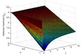
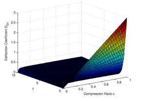
Figure 5: Modified Deflection Coefficient analysis. 5 DFCsubscript𝐷𝐹𝐶D_{FC} with varying c𝑐c and κ𝜅\kappa. 5 DEVsubscript𝐷𝐸𝑉D_{EV} with varying c𝑐c and κ𝜅\kappa.
Refer to caption
Refer to caption
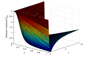
Figure 6: Modified Deflection Coefficient analysis. 6 DFCsubscript𝐷𝐹𝐶D_{FC} with varying α𝛼\alpha and κ𝜅\kappa. 6 DEVsubscript𝐷𝐸𝑉D_{EV} with varying α𝛼\alpha and κ𝜅\kappa.

V-A Performance Analysis of Collaborative Compressive Detection with an Eavesdropper

First, we derive closed form expressions of the modified deflection coefficients at the FC.

V-A1 A Closed Form Expression of the Modified Deflection Coefficient at the FC

As stated earlier, the modified deflection coefficient at the FC is

DFC=αD(yi~)+(1α)D(yi).subscript𝐷𝐹𝐶𝛼𝐷~subscript𝑦𝑖1𝛼𝐷subscript𝑦𝑖D_{FC}=\alpha D(\tilde{y_{i}})+(1-\alpha)D(y_{i}).

It can be shown that

D(yi)=P^μ22γ1+β1,𝐷subscript𝑦𝑖superscriptsubscriptnorm^𝑃𝜇22superscript𝛾1superscript𝛽1D(y_{i})=\dfrac{\|\hat{P}\mu\|_{2}^{2}}{\gamma^{-1}+\beta^{-1}},

where P^=ϕT(ϕϕT)ϕ^𝑃superscriptitalic-ϕ𝑇italic-ϕsuperscriptitalic-ϕ𝑇italic-ϕ\hat{P}=\phi^{T}(\phi\phi^{T})\phi.

Next, to derive D(yi~)𝐷~subscript𝑦𝑖D(\tilde{y_{i}}), observe that yi~~subscript𝑦𝑖\tilde{y_{i}} is distributed as a multivariate Gaussian mixture with

μ~0isuperscriptsubscript~𝜇0𝑖\displaystyle\tilde{\mu}_{0}^{i} =\displaystyle= (P10P20)ϕDisuperscriptsubscript𝑃10superscriptsubscript𝑃20italic-ϕsubscript𝐷𝑖\displaystyle(P_{1}^{0}-P_{2}^{0})\phi D_{i}
μ~1isuperscriptsubscript~𝜇1𝑖\displaystyle\tilde{\mu}_{1}^{i} =\displaystyle= (P11P21)ϕDi+ϕμsuperscriptsubscript𝑃11superscriptsubscript𝑃21italic-ϕsubscript𝐷𝑖italic-ϕ𝜇\displaystyle(P_{1}^{1}-P_{2}^{1})\phi D_{i}+\phi\mu
Σ~1isuperscriptsubscript~Σ1𝑖\displaystyle\tilde{\Sigma}_{1}^{i} =\displaystyle= σ2ϕϕT+j=13Pj1(μ~1i(j)μ~1i)(μ~1i(j)μ~1i)Tsuperscript𝜎2italic-ϕsuperscriptitalic-ϕ𝑇superscriptsubscript𝑗13superscriptsubscript𝑃𝑗1superscriptsubscript~𝜇1𝑖𝑗superscriptsubscript~𝜇1𝑖superscriptsuperscriptsubscript~𝜇1𝑖𝑗superscriptsubscript~𝜇1𝑖𝑇\displaystyle\sigma^{2}\phi\phi^{T}+\sum_{j=1}^{3}P_{j}^{1}(\tilde{\mu}_{1}^{i}(j)-\tilde{\mu}_{1}^{i})(\tilde{\mu}_{1}^{i}(j)-\tilde{\mu}_{1}^{i})^{T}

where μ~1i(1)=ϕ(μ+Di)superscriptsubscript~𝜇1𝑖1italic-ϕ𝜇subscript𝐷𝑖\tilde{\mu}_{1}^{i}(1)=\phi(\mu+D_{i}), μ~1i(2)=ϕ(μDi)superscriptsubscript~𝜇1𝑖2italic-ϕ𝜇subscript𝐷𝑖\tilde{\mu}_{1}^{i}(2)=\phi(\mu-D_{i}), μ~1i(3)=ϕμsuperscriptsubscript~𝜇1𝑖3italic-ϕ𝜇\tilde{\mu}_{1}^{i}(3)=\phi\mu, P31=1P11P21superscriptsubscript𝑃311superscriptsubscript𝑃11superscriptsubscript𝑃21P_{3}^{1}=1-P_{1}^{1}-P_{2}^{1} and σ2=(α1+β1+γ1)superscript𝜎2superscript𝛼1superscript𝛽1superscript𝛾1\sigma^{2}=(\alpha^{-1}+\beta^{-1}+\gamma^{-1}). After some derivation, it can be shown that

Σ~1i=σ2ϕϕT+Pt[ϕDiDiTϕT]superscriptsubscript~Σ1𝑖superscript𝜎2italic-ϕsuperscriptitalic-ϕ𝑇subscript𝑃𝑡delimited-[]italic-ϕsubscript𝐷𝑖superscriptsubscript𝐷𝑖𝑇superscriptitalic-ϕ𝑇\tilde{\Sigma}_{1}^{i}=\sigma^{2}\phi\phi^{T}+P_{t}[\phi D_{i}D_{i}^{T}\phi^{T}]

where Pt=P11+P21(P11P21)2subscript𝑃𝑡superscriptsubscript𝑃11superscriptsubscript𝑃21superscriptsuperscriptsubscript𝑃11superscriptsubscript𝑃212P_{t}=P_{1}^{1}+P_{2}^{1}-(P_{1}^{1}-P_{2}^{1})^{2}. Also, notice that Σ~1isuperscriptsubscript~Σ1𝑖\tilde{\Sigma}_{1}^{i} is of the form A+bbT𝐴𝑏superscript𝑏𝑇A+bb^{T}. Now, using the Sherman-Morrison formula [27], its inverse can be obtained to be

(Σ~1i)1=(ϕϕT)1σ2Pt(ϕϕT)1ϕDiDiTϕT(ϕϕT)1σ4+σ2PtDiTϕT(ϕϕT)1ϕDisuperscriptsuperscriptsubscript~Σ1𝑖1superscriptitalic-ϕsuperscriptitalic-ϕ𝑇1superscript𝜎2subscript𝑃𝑡superscriptitalic-ϕsuperscriptitalic-ϕ𝑇1italic-ϕsubscript𝐷𝑖superscriptsubscript𝐷𝑖𝑇superscriptitalic-ϕ𝑇superscriptitalic-ϕsuperscriptitalic-ϕ𝑇1superscript𝜎4superscript𝜎2subscript𝑃𝑡superscriptsubscript𝐷𝑖𝑇superscriptitalic-ϕ𝑇superscriptitalic-ϕsuperscriptitalic-ϕ𝑇1italic-ϕsubscript𝐷𝑖(\tilde{\Sigma}_{1}^{i})^{-1}=\frac{(\phi\phi^{T})^{-1}}{\sigma^{2}}-\frac{P_{t}(\phi\phi^{T})^{-1}\phi D_{i}D_{i}^{T}\phi^{T}(\phi\phi^{T})^{-1}}{\sigma^{4}+\sigma^{2}P_{t}D_{i}^{T}\phi^{T}(\phi\phi^{T})^{-1}\phi D_{i}} (17)

with σ2=(α1+β1+γ1)superscript𝜎2superscript𝛼1superscript𝛽1superscript𝛾1\sigma^{2}=(\alpha^{-1}+\beta^{-1}+\gamma^{-1}).

Also,

(μ~1iμ~0i)=ϕμPbϕDisuperscriptsubscript~𝜇1𝑖superscriptsubscript~𝜇0𝑖italic-ϕ𝜇subscript𝑃𝑏italic-ϕsubscript𝐷𝑖(\tilde{\mu}_{1}^{i}-\tilde{\mu}_{0}^{i})=\phi\mu-P_{b}\phi D_{i} (18)

where Pb=(P10P20)+(P21P11)subscript𝑃𝑏superscriptsubscript𝑃10superscriptsubscript𝑃20superscriptsubscript𝑃21superscriptsubscript𝑃11P_{b}=(P_{1}^{0}-P_{2}^{0})+(P_{2}^{1}-P_{1}^{1}). Using (17), (18) and the fact that Di=κμsubscript𝐷𝑖𝜅𝜇D_{i}=\kappa\mu where κ𝜅\kappa is referred to as the noise strength, the modified deflection coefficient D(yi~)𝐷~subscript𝑦𝑖D(\tilde{y_{i}}) can be derived to be333For μ=0𝜇0\mu=0, DFCαPb2Pt+σ2P^dsubscript𝐷𝐹𝐶𝛼superscriptsubscript𝑃𝑏2subscript𝑃𝑡superscript𝜎2norm^𝑃𝑑D_{FC}\approx\alpha\frac{P_{b}^{2}}{P_{t}+\frac{\sigma^{2}}{\|\hat{P}d\|}} where Di=d,isubscript𝐷𝑖𝑑for-all𝑖D_{i}=d,\forall i.

D(yi~)=(1Pbκ)2P^μ22σ2Ptγ2(1Pbκ)2P^μ24σ2rb𝐷~subscript𝑦𝑖superscript1subscript𝑃𝑏𝜅2superscriptsubscriptnorm^𝑃𝜇22superscript𝜎2subscript𝑃𝑡superscript𝛾2superscript1subscript𝑃𝑏𝜅2superscriptsubscriptnorm^𝑃𝜇24superscript𝜎2subscript𝑟𝑏D(\tilde{y_{i}})=(1-P_{b}\kappa)^{2}\frac{\|\hat{P}\mu\|_{2}^{2}}{\sigma^{2}}-P_{t}\gamma^{2}(1-P_{b}\kappa)^{2}\frac{\|\hat{P}\mu\|_{2}^{4}}{\sigma^{2}r_{b}} (19)

where rb=σ2+Ptκ2P^μ22subscript𝑟𝑏superscript𝜎2subscript𝑃𝑡superscript𝜅2superscriptsubscriptnorm^𝑃𝜇22r_{b}=\sigma^{2}+P_{t}\kappa^{2}\|\hat{P}\mu\|_{2}^{2} and σ2=(α1+β1+γ1)superscript𝜎2superscript𝛼1superscript𝛽1superscript𝛾1\sigma^{2}=(\alpha^{-1}+\beta^{-1}+\gamma^{-1}).

Proposition 2.

Suppose that PMP^𝑃𝑀^𝑃\sqrt{\frac{P}{M}}\hat{P} provides an ϵitalic-ϵ\epsilon-stable embedding of (𝒰,{0})𝒰0(\mathcal{U},\{0\}). Then the modified deflection coefficient at the FC for any μ𝒰𝜇𝒰\mu\in\mathcal{U} can be approximated as

DFCα(1Pbκ)2κ2Pt+c1σ2μ22+(1α)cμ22σ2subscript𝐷𝐹𝐶𝛼superscript1subscript𝑃𝑏𝜅2superscript𝜅2subscript𝑃𝑡superscript𝑐1superscript𝜎2superscriptsubscriptnorm𝜇221𝛼𝑐superscriptsubscriptnorm𝜇22superscript𝜎2D_{FC}\approx\alpha\frac{(1-P_{b}\kappa)^{2}}{\kappa^{2}P_{t}+c^{-1}\frac{\sigma^{2}}{\|\mu\|_{2}^{2}}}+(1-\alpha)c\frac{\|\mu\|_{2}^{2}}{\sigma^{2}} (20)

where

Pb=(P10P20)+(P21P11)subscript𝑃𝑏superscriptsubscript𝑃10superscriptsubscript𝑃20superscriptsubscript𝑃21superscriptsubscript𝑃11P_{b}=(P_{1}^{0}-P_{2}^{0})+(P_{2}^{1}-P_{1}^{1}), Pt=P11+P21(P11P21)2subscript𝑃𝑡superscriptsubscript𝑃11superscriptsubscript𝑃21superscriptsuperscriptsubscript𝑃11superscriptsubscript𝑃212P_{t}=P_{1}^{1}+P_{2}^{1}-(P_{1}^{1}-P_{2}^{1})^{2} and σ2=(α1+β1+γ1)superscript𝜎2superscript𝛼1superscript𝛽1superscript𝛾1\sigma^{2}=(\alpha^{-1}+\beta^{-1}+\gamma^{-1}).

Proof.

Using the fact that PMP^𝑃𝑀^𝑃\sqrt{\frac{P}{M}}\hat{P} provides an ϵitalic-ϵ\epsilon-stable embedding of (U,{0})𝑈0(U,\{0\}), for any μ𝒰𝜇𝒰\mu\in\mathcal{U}, D(yi)𝐷subscript𝑦𝑖D(y_{i}) and D(y~i)𝐷subscript~𝑦𝑖D(\tilde{y}_{i}) can be approximated as

D(yi)𝐷subscript𝑦𝑖\displaystyle D(y_{i}) =\displaystyle= MPμ22σ2𝑀𝑃superscriptsubscriptnorm𝜇22superscript𝜎2\displaystyle\frac{M}{P}\frac{\|\mu\|_{2}^{2}}{\sigma^{2}}
D(y~i)𝐷subscript~𝑦𝑖\displaystyle D(\tilde{y}_{i}) =\displaystyle= MPμ22σ2(1Pbκ)2(1MPμ22rbκ2Pt)𝑀𝑃superscriptsubscriptnorm𝜇22superscript𝜎2superscript1subscript𝑃𝑏𝜅21𝑀𝑃superscriptsubscriptnorm𝜇22subscript𝑟𝑏superscript𝜅2subscript𝑃𝑡\displaystyle\frac{M}{P}\frac{\|\mu\|_{2}^{2}}{\sigma^{2}}(1-P_{b}\kappa)^{2}\left(1-\frac{M}{P}\frac{\|\mu\|_{2}^{2}}{r_{b}}\kappa^{2}P_{t}\right)

where rb=σ2+Ptκ2P^μ22subscript𝑟𝑏superscript𝜎2subscript𝑃𝑡superscript𝜅2superscriptsubscriptnorm^𝑃𝜇22r_{b}=\sigma^{2}+P_{t}\kappa^{2}\|\hat{P}\mu\|_{2}^{2} and σ2=(α1+β1+γ1)superscript𝜎2superscript𝛼1superscript𝛽1superscript𝛾1\sigma^{2}=(\alpha^{-1}+\beta^{-1}+\gamma^{-1}). Plugging in the above values in DFC=αD(yi~)+(1α)D(yi)subscript𝐷𝐹𝐶𝛼𝐷~subscript𝑦𝑖1𝛼𝐷subscript𝑦𝑖D_{FC}=\alpha D(\tilde{y_{i}})+(1-\alpha)D(y_{i}) yields the desired result. ∎

Next, we derive the modified deflection coefficient at the eavesdropper.

V-A2 A Closed Form Expression of the Modified Deflection Coefficients at the Eavesdropper

As stated earlier, the modified deflection coefficient of the eavesdropper is

DEV=D(yi^).subscript𝐷𝐸𝑉𝐷^subscript𝑦𝑖D_{EV}=D(\hat{y_{i}}).

Next, to derive D(yi^)𝐷^subscript𝑦𝑖D(\hat{y_{i}}), observe that yi^^subscript𝑦𝑖\hat{y_{i}} is distributed as a multivariate Gaussian mixture with

μ^0isuperscriptsubscript^𝜇0𝑖\displaystyle\hat{\mu}_{0}^{i} =\displaystyle= α(P10P20)ϕDi𝛼superscriptsubscript𝑃10superscriptsubscript𝑃20italic-ϕsubscript𝐷𝑖\displaystyle\alpha(P_{1}^{0}-P_{2}^{0})\phi D_{i}
μ^1isuperscriptsubscript^𝜇1𝑖\displaystyle\hat{\mu}_{1}^{i} =\displaystyle= α(P11P21)ϕDi+ϕμ𝛼superscriptsubscript𝑃11superscriptsubscript𝑃21italic-ϕsubscript𝐷𝑖italic-ϕ𝜇\displaystyle\alpha(P_{1}^{1}-P_{2}^{1})\phi D_{i}+\phi\mu
Σ^1isuperscriptsubscript^Σ1𝑖\displaystyle\hat{\Sigma}_{1}^{i} =\displaystyle= σ2ϕϕT+j=13pj1(μ^1i(j)μ^1i)(μ^1i(j)μ^1i)Tsuperscript𝜎2italic-ϕsuperscriptitalic-ϕ𝑇superscriptsubscript𝑗13superscriptsubscript𝑝𝑗1superscriptsubscript^𝜇1𝑖𝑗superscriptsubscript^𝜇1𝑖superscriptsuperscriptsubscript^𝜇1𝑖𝑗superscriptsubscript^𝜇1𝑖𝑇\displaystyle\sigma^{2}\phi\phi^{T}+\sum_{j=1}^{3}p_{j}^{1}(\hat{\mu}_{1}^{i}(j)-\hat{\mu}_{1}^{i})(\hat{\mu}_{1}^{i}(j)-\hat{\mu}_{1}^{i})^{T}

with μ^1i(1)=ϕ(μ+Di)superscriptsubscript^𝜇1𝑖1italic-ϕ𝜇subscript𝐷𝑖\hat{\mu}_{1}^{i}(1)=\phi(\mu+D_{i}), μ^1i(2)=ϕ(μDi)superscriptsubscript^𝜇1𝑖2italic-ϕ𝜇subscript𝐷𝑖\hat{\mu}_{1}^{i}(2)=\phi(\mu-D_{i}), μ^1i(3)=ϕμsuperscriptsubscript^𝜇1𝑖3italic-ϕ𝜇\hat{\mu}_{1}^{i}(3)=\phi\mu, p11=αP11superscriptsubscript𝑝11𝛼superscriptsubscript𝑃11p_{1}^{1}=\alpha P_{1}^{1}, p21=αP21superscriptsubscript𝑝21𝛼superscriptsubscript𝑃21p_{2}^{1}=\alpha P_{2}^{1}, p31=1α(P11P21)superscriptsubscript𝑝311𝛼superscriptsubscript𝑃11superscriptsubscript𝑃21p_{3}^{1}=1-\alpha(P_{1}^{1}-P_{2}^{1}) and σ2=(α1+γ1+β1)superscript𝜎2superscript𝛼1superscript𝛾1superscript𝛽1\sigma^{2}=(\alpha^{-1}+\gamma^{-1}+\beta^{-1}). Using these values, we state our result in the next proposition.444For μ=0𝜇0\mu=0, DEV(αPb)2αPtE+σ2P^dsubscript𝐷𝐸𝑉superscript𝛼subscript𝑃𝑏2𝛼superscriptsubscript𝑃𝑡𝐸superscript𝜎2norm^𝑃𝑑D_{EV}\approx\frac{(\alpha P_{b})^{2}}{\alpha P_{t}^{E}+\frac{\sigma^{2}}{\|\hat{P}d\|}} where Di=d,isubscript𝐷𝑖𝑑for-all𝑖D_{i}=d,\forall i.

Proposition 3.

Suppose that PMP^𝑃𝑀^𝑃\sqrt{\frac{P}{M}}\hat{P} provides an ϵitalic-ϵ\epsilon-stable embedding of (𝒰,{0})𝒰0(\mathcal{U},\{0\}). Then, the modified deflection coefficient at the eavesdropper for any μ𝒰𝜇𝒰\mu\in\mathcal{U} can be approximated as

DEV(1αPbκ)2ακ2PtE+c1σ2μ22subscript𝐷𝐸𝑉superscript1𝛼subscript𝑃𝑏𝜅2𝛼superscript𝜅2superscriptsubscript𝑃𝑡𝐸superscript𝑐1superscript𝜎2superscriptsubscriptnorm𝜇22D_{EV}\approx\frac{(1-\alpha P_{b}\kappa)^{2}}{\alpha\kappa^{2}P_{t}^{E}+c^{-1}\frac{\sigma^{2}}{\|\mu\|_{2}^{2}}} (21)

where

Pb=(P10P20)+(P21P11)subscript𝑃𝑏superscriptsubscript𝑃10superscriptsubscript𝑃20superscriptsubscript𝑃21superscriptsubscript𝑃11P_{b}=(P_{1}^{0}-P_{2}^{0})+(P_{2}^{1}-P_{1}^{1}), PtE=P11+P21α(P11P21)2superscriptsubscript𝑃𝑡𝐸superscriptsubscript𝑃11superscriptsubscript𝑃21𝛼superscriptsuperscriptsubscript𝑃11superscriptsubscript𝑃212P_{t}^{E}=P_{1}^{1}+P_{2}^{1}-\alpha(P_{1}^{1}-P_{2}^{1})^{2} and σ2=(α1+β1+γ1)superscript𝜎2superscript𝛼1superscript𝛽1superscript𝛾1\sigma^{2}=(\alpha^{-1}+\beta^{-1}+\gamma^{-1}).

Proof.

The proof is similar to that of Proposition 2 and is, therefore, omitted. ∎

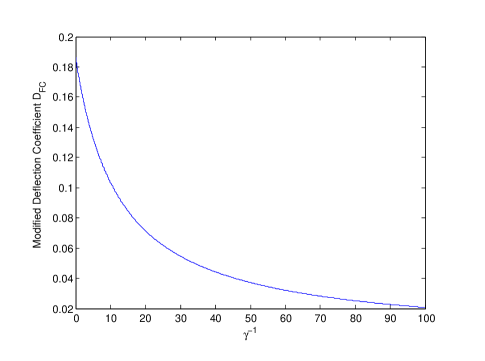
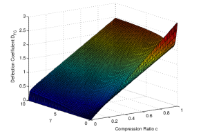
In general, there is a trade-off between the detection performance and the security performance of the system. To gain insights into this trade-off, in Figure 5 we plot the modified deflection coefficient, both at the FC and at the eavesdropper, as a function of compression ratio (c)𝑐(c) and noise strength (κ)𝜅(\kappa) when α=0.3,P10=P21=0.8,P20=P11=0.1formulae-sequenceformulae-sequence𝛼0.3superscriptsubscript𝑃10superscriptsubscript𝑃210.8superscriptsubscript𝑃20superscriptsubscript𝑃110.1\alpha=0.3,\;P_{1}^{0}=P_{2}^{1}=0.8,\;P_{2}^{0}=P_{1}^{1}=0.1 and μ22σ2=3superscriptsubscriptnorm𝜇22superscript𝜎23\frac{\|\mu\|_{2}^{2}}{\sigma^{2}}=3. Next, in Figure 6 we plot the modified deflection coefficient, both at the FC and at the eavesdropper, as a function of the fraction of artificial noise injecting nodes (α)𝛼(\alpha) and noise strength (κ)𝜅(\kappa) when P10=P21=0.8,P20=P11=0.1formulae-sequencesuperscriptsubscript𝑃10superscriptsubscript𝑃210.8superscriptsubscript𝑃20superscriptsubscript𝑃110.1P_{1}^{0}=P_{2}^{1}=0.8,\;P_{2}^{0}=P_{1}^{1}=0.1 and MPμ22σ2=3𝑀𝑃superscriptsubscriptnorm𝜇22superscript𝜎23\frac{M}{P}\frac{\|\mu\|_{2}^{2}}{\sigma^{2}}=3. It can be seen from Figure 5 and Figure 6 that DFCsubscript𝐷𝐹𝐶D_{FC} and DEVsubscript𝐷𝐸𝑉D_{EV} do not exhibit nice properties (monotonicity or convexity) with respect to the system parameters and, therefore, it is not an easy task to design the system parameters under an arbitrary physical layer secrecy constraint. Also notice that, a specific case where the eavesdropper is completely blind deserves particular attention. This is referred to as the perfect secrecy regime, i.e., DEV=0subscript𝐷𝐸𝑉0D_{EV}=0. In the next subsection, we explore the problem of system design in a holistic manner in the perfect secrecy regime. More specifically, we are interested in analyzing the behavior of the modified deflection coefficient, both at the FC and at the eavesdropper, as a function of compression ratio (c=M/P)𝑐𝑀𝑃(c=M/P) and artificial noise injection parameters (α,Wi)𝛼subscript𝑊𝑖(\alpha,W_{i}).

V-B Optimal System Design Under Perfect Secrecy Constraint

The goal of the designer is to maximize the detection performance DFCsubscript𝐷𝐹𝐶D_{FC}, while ensuring perfect secrecy at the eavesdropper. The system design problem under perfect secrecy constraint can be formally stated as:

maximizec,α,Wi𝑐𝛼subscript𝑊𝑖maximize\displaystyle\underset{c,\alpha,W_{i}}{\text{maximize}} αD(yi~)+(1α)D(yi)𝛼𝐷~subscript𝑦𝑖1𝛼𝐷subscript𝑦𝑖\displaystyle\alpha D(\tilde{y_{i}})+(1-\alpha)D(y_{i}) (22)
subject to D(yi^)=0𝐷^subscript𝑦𝑖0\displaystyle D(\hat{y_{i}})=0

where c𝑐c is the compression ratio and (α,Wi)𝛼subscript𝑊𝑖(\alpha,\;W_{i}) are the artificial noise injection parameters. This reduction of the search space, which arises as a natural consequence of the perfect secrecy constraint, has the additional benefit of simplifying the mathematical analysis. Next, we first explore the answer to the question: Does compression help in improving the security performance of the system?

V-B1 Does Compression Help?

We first consider the case where αPbκ1𝛼subscript𝑃𝑏𝜅1\alpha P_{b}\kappa\neq 1. In this regime, for fixed values of α𝛼\alpha, Pbsubscript𝑃𝑏P_{b} and κ𝜅\kappa, the modified deflection coefficient, both at the FC and the eavesdropper, is a monotonically increasing function of the compression ratio. In other words, dDFCdc>0𝑑subscript𝐷𝐹𝐶𝑑𝑐0\frac{dD_{FC}}{dc}>0 and dDEVdc>0𝑑subscript𝐷𝐸𝑉𝑑𝑐0\frac{dD_{EV}}{dc}>0. This suggests that compression improves the security performance at the expense of detection performance. More specifically, the FC would decrease the compression ratio until the physical layer secrecy constraint is satisfied. As a consequence, it will result in performance loss at the FC due to compression. In other words, there is a trade-off between the detection performance and the security performance of the system. Observe that, DEV=0subscript𝐷𝐸𝑉0D_{EV}=0 if and only if αPbκ=1𝛼subscript𝑃𝑏𝜅1\alpha P_{b}\kappa=1 (ignoring the extreme conditions such as c=0𝑐0c=0 or κ=𝜅\kappa=\infty) and, in this regime, DFCsubscript𝐷𝐹𝐶D_{FC} is a monotonically increasing function of the compression ratio c𝑐c and DEVsubscript𝐷𝐸𝑉D_{EV} is independent of the compression ratio c𝑐c. These results are summarized in the the following proposition.

Proposition 4.

In the perfect secrecy regime (i.e.,αPbκ=1)(i.e.,\alpha P_{b}\kappa=1), DFCsubscript𝐷𝐹𝐶D_{FC} is a monotonically increasing function of the compression ratio c𝑐c and DEVsubscript𝐷𝐸𝑉D_{EV} is independent of the compression ratio c𝑐c. When αPbκ1𝛼subscript𝑃𝑏𝜅1\alpha P_{b}\kappa\neq 1, the modified deflection coefficient, both at the FC and the eavesdropper, is a monotonically increasing function of the compression ratio.

As mentioned above, in the perfect secrecy regime DEVsubscript𝐷𝐸𝑉D_{EV} is independent of the compression ratio c𝑐c and the network designer can fix c=cmax𝑐subscript𝑐𝑚𝑎𝑥c=c_{max}, where the value of cmaxsubscript𝑐𝑚𝑎𝑥c_{max} may be dependent on the application of interest. The system design problem under perfect secrecy constraint can be reformulated as

argmaxα,WiDFC(cmax,κ=1/(Pbα)).𝛼subscript𝑊𝑖subscript𝐷𝐹𝐶subscript𝑐𝑚𝑎𝑥𝜅1subscript𝑃𝑏𝛼\underset{\alpha,W_{i}}{\arg\max}\;D_{FC}(c_{max},\kappa=1/(P_{b}\alpha)). (23)

Next, we analyze the behavior of the DFC(cmax,κ=1/(Pbα))subscript𝐷𝐹𝐶subscript𝑐𝑚𝑎𝑥𝜅1subscript𝑃𝑏𝛼D_{FC}(c_{max},\kappa=1/(P_{b}\alpha)) as a function of artificial noise injection parameters (α,Wi)𝛼subscript𝑊𝑖(\alpha,W_{i}).

V-B2 Optimal Artificial Noise Injection Parameters
Refer to caption
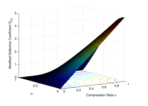
Figure 7: Modified Deflection Coefficient as a function of α𝛼\alpha and compression ratio c=M/P𝑐𝑀𝑃c=M/P for SNR=5𝑆𝑁𝑅5SNR=5dB in perfect secrecy regime.
Proposition 5.

In the high signal to noise ratio regime (defined as μ22σ2>Pb2Ptsuperscriptsubscriptnorm𝜇22superscript𝜎2superscriptsubscript𝑃𝑏2subscript𝑃𝑡\frac{\|\mu\|_{2}^{2}}{\sigma^{2}}>\frac{P_{b}^{2}}{P_{t}} where σ2=(α1+γ1+β1)superscript𝜎2superscript𝛼1superscript𝛾1superscript𝛽1\sigma^{2}=(\alpha^{-1}+\gamma^{-1}+\beta^{-1})), the modified deflection coefficient at the FC, DFCsubscript𝐷𝐹𝐶D_{FC}, is a monotonically decreasing function of the fraction of data falsifying nodes (0<α10𝛼10<\alpha\leq 1) under the perfect secrecy constraint.

Proof.

Deflection coefficient at the FC under the perfect secrecy constraint can be expressed as

DFC(cmax,κ=1/(Pbα))=α(11α)2Ptα2Pb2+1D+(1α)Dsubscript𝐷𝐹𝐶subscript𝑐𝑚𝑎𝑥𝜅1subscript𝑃𝑏𝛼𝛼superscript11𝛼2subscript𝑃𝑡superscript𝛼2superscriptsubscript𝑃𝑏21𝐷1𝛼𝐷D_{FC}(c_{max},\kappa=1/(P_{b}\alpha))=\frac{\alpha(1-\frac{1}{\alpha})^{2}}{\frac{P_{t}}{\alpha^{2}P_{b}^{2}}+\frac{1}{D}}+(1-\alpha)D

with D=cmaxμ22σ2𝐷subscript𝑐𝑚𝑎𝑥superscriptsubscriptnorm𝜇22superscript𝜎2D=c_{max}\frac{\|\mu\|_{2}^{2}}{\sigma^{2}}. Now, deriving the derivative of DFCsubscript𝐷𝐹𝐶D_{FC} with respect to α𝛼\alpha results in

dDFCdα=PtPb2D2(14α+α2)DPb4α2Pt2D3(PtD+α2Pb2)2.𝑑subscript𝐷𝐹𝐶𝑑𝛼subscript𝑃𝑡superscriptsubscript𝑃𝑏2superscript𝐷214𝛼superscript𝛼2𝐷superscriptsubscript𝑃𝑏4superscript𝛼2superscriptsubscript𝑃𝑡2superscript𝐷3superscriptsubscript𝑃𝑡𝐷superscript𝛼2superscriptsubscript𝑃𝑏22\frac{dD_{FC}}{d\alpha}=\frac{P_{t}P_{b}^{2}D^{2}(1-4\alpha+\alpha^{2})-DP_{b}^{4}\alpha^{2}-P_{t}^{2}D^{3}}{(P_{t}D+\alpha^{2}P_{b}^{2})^{2}}.

Next, we show that dDFCdα<0𝑑subscript𝐷𝐹𝐶𝑑𝛼0\frac{dD_{FC}}{d\alpha}<0.

First, let us define F(α)=x+α21x(1+α2)𝐹𝛼𝑥superscript𝛼21𝑥1superscript𝛼2F(\alpha)=x+\alpha^{2}\frac{1}{x}-(1+\alpha^{2}). It is easy to show that F(α)𝐹𝛼F(\alpha) is a decreasing function of α𝛼\alpha if x>1𝑥1x>1. This also implies that F(α)>0𝐹𝛼0F(\alpha)>0 if and only if F(α=1)>0(x+1x)>2𝐹𝛼10𝑥1𝑥2F(\alpha=1)>0\Leftrightarrow(x+\frac{1}{x})>2. Note that, (x+1x)>2𝑥1𝑥2(x+\frac{1}{x})>2, which follows from the fact that arithmetic mean is greater than the geometric mean. Having shown that F(α)>0𝐹𝛼0F(\alpha)>0, we return back to showing that dDFCdα<0𝑑subscript𝐷𝐹𝐶𝑑𝛼0\frac{dD_{FC}}{d\alpha}<0. We start with the inequality

x+α21x(1+α2)>0𝑥superscript𝛼21𝑥1superscript𝛼20\displaystyle x+\alpha^{2}\frac{1}{x}-(1+\alpha^{2})>0
\displaystyle\Leftrightarrow x+α21x>(1+α2)𝑥superscript𝛼21𝑥1superscript𝛼2\displaystyle x+\alpha^{2}\frac{1}{x}>(1+\alpha^{2})
\displaystyle\Rightarrow 4α(1+α2)+x(1+α2)+α2(1+α2)1x>14𝛼1superscript𝛼2𝑥1superscript𝛼2superscript𝛼21superscript𝛼21𝑥1\displaystyle\frac{4\alpha}{(1+\alpha^{2})}+\frac{x}{(1+\alpha^{2})}+\frac{\alpha^{2}}{(1+\alpha^{2})}\frac{1}{x}>1

Now, if we plug in x=DPtPB2𝑥𝐷subscript𝑃𝑡superscriptsubscript𝑃𝐵2x=D\frac{P_{t}}{P_{B}^{2}} in the above inequality and rearrange the terms we get

PtPb2D2(14α+α2)DPb4α2Pt2D3(PtD+α2Pb2)2<0subscript𝑃𝑡superscriptsubscript𝑃𝑏2superscript𝐷214𝛼superscript𝛼2𝐷superscriptsubscript𝑃𝑏4superscript𝛼2superscriptsubscript𝑃𝑡2superscript𝐷3superscriptsubscript𝑃𝑡𝐷superscript𝛼2superscriptsubscript𝑃𝑏220\frac{P_{t}P_{b}^{2}D^{2}(1-4\alpha+\alpha^{2})-DP_{b}^{4}\alpha^{2}-P_{t}^{2}D^{3}}{(P_{t}D+\alpha^{2}P_{b}^{2})^{2}}<0

which is true if x=DPtPB2>1𝑥𝐷subscript𝑃𝑡superscriptsubscript𝑃𝐵21x=D\frac{P_{t}}{P_{B}^{2}}>1. ∎

Notice that, Proposition 4 suggests that to maximize the modified deflection coefficient DFCsubscript𝐷𝐹𝐶D_{FC} under the perfect secrecy constraint (22), the network designer should choose the value of α𝛼\alpha as low as possible under the constraint that α>0𝛼0\alpha>0 and accordingly increase κ𝜅\kappa to satisfy αPbκ=1𝛼subscript𝑃𝑏𝜅1\alpha P_{b}\kappa=1. In practice, αminsubscript𝛼𝑚𝑖𝑛\alpha_{min} may be dependent on the application of interest.

Next, to gain insights into Proposition 4 and 5, we present illustrative examples that corroborate our results. In Figure 7, we plot DFCsubscript𝐷𝐹𝐶D_{FC} as a function of fraction of noise injection nodes α𝛼\alpha and compression ratio c𝑐c in the perfect secrecy regime when P10=P21=0.8,P20=P11=0.1formulae-sequencesuperscriptsubscript𝑃10superscriptsubscript𝑃210.8superscriptsubscript𝑃20superscriptsubscript𝑃110.1P_{1}^{0}=P_{2}^{1}=0.8,\;P_{2}^{0}=P_{1}^{1}=0.1 and μ22σ2=5dBsuperscriptsubscriptnorm𝜇22superscript𝜎25𝑑𝐵\frac{\|\mu\|_{2}^{2}}{\sigma^{2}}=5dB. It can be seen from the figure that DFCsubscript𝐷𝐹𝐶D_{FC} is a monotonically increasing function of c𝑐c and a monotonically decreasing function of α𝛼\alpha.

Next, we analyze the behavior of DFCsubscript𝐷𝐹𝐶D_{FC} as a function of artificial noise variance γ1superscript𝛾1\gamma^{-1}. This analysis will help us in determining the optimal artificial noise injection parameters.

Proposition 6.

In the high signal to noise ratio regime (defined as μ22σ2>Pb2Ptsuperscriptsubscriptnorm𝜇22superscript𝜎2superscriptsubscript𝑃𝑏2subscript𝑃𝑡\frac{\|\mu\|_{2}^{2}}{\sigma^{2}}>\frac{P_{b}^{2}}{P_{t}} where σ2=(α1+γ1+β1)superscript𝜎2superscript𝛼1superscript𝛾1superscript𝛽1\sigma^{2}=(\alpha^{-1}+\gamma^{-1}+\beta^{-1})) with perfect secrecy constraint (i.e.,αPbκ=1)(i.e.,\;\alpha P_{b}\kappa=1), the optimal artificial noise is a deterministic signal with value μαminPb𝜇subscript𝛼𝑚𝑖𝑛subscript𝑃𝑏\frac{\mu}{\alpha_{min}P_{b}}, i.e., fWi(wi)=δ(wiμαminPb)subscript𝑓subscript𝑊𝑖subscript𝑤𝑖𝛿subscript𝑤𝑖𝜇subscript𝛼𝑚𝑖𝑛subscript𝑃𝑏f_{W_{i}}(w_{i})=\delta(w_{i}-\frac{\mu}{\alpha_{min}P_{b}}).

Proof.

The proof follows from Proposition 5 and the fact that DFCsubscript𝐷𝐹𝐶D_{FC} is a monotonically decreasing function of the variance γ1superscript𝛾1\gamma^{-1} of the artificial noise, i.e., dDFCdγ1<0𝑑subscript𝐷𝐹𝐶𝑑superscript𝛾10\frac{dD_{FC}}{d\gamma^{-1}}<0. ∎

Refer to caption
Figure 8: Modified Deflection Coefficient as a function of γ1superscript𝛾1\gamma^{-1} in perfect secrecy regime.

In Figure 8, we plot the modified deflection coefficient at the FC as a function of the variance of the artificial noise when P10=P21=0.8,P20=P11=0.1formulae-sequencesuperscriptsubscript𝑃10superscriptsubscript𝑃210.8superscriptsubscript𝑃20superscriptsubscript𝑃110.1P_{1}^{0}=P_{2}^{1}=0.8,\;P_{2}^{0}=P_{1}^{1}=0.1 and (c,α)=(0.2,0.3)𝑐𝛼0.20.3(c,\alpha)=(0.2,0.3). We assume that the signal of interest is s𝒩(μ,IP)similar-to𝑠𝒩𝜇subscript𝐼𝑃s\sim\mathcal{N}(\mu,I_{P}) with μ22=5superscriptsubscriptnorm𝜇225\|\mu\|_{2}^{2}=5 and noise vi𝒩(0,10IP)similar-tosubscript𝑣𝑖𝒩010subscript𝐼𝑃v_{i}\sim\mathcal{N}(0,10I_{P}). It can be seen that DFCsubscript𝐷𝐹𝐶D_{FC} is a monotonically decreasing function of the artificial noise variance γ1superscript𝛾1\gamma^{-1}. This observation implies that the optimal artificial noise is a deterministic signal. Using these results, the solution of the optimization problem (22) is summarized in the following theorem.

Theorem 4.

To maximize the modified deflection coefficient at the FC under the perfect secrecy constraint, the network designer should choose c=cmax𝑐subscript𝑐𝑚𝑎𝑥c=c_{max}, α=αmin𝛼subscript𝛼𝑚𝑖𝑛\alpha=\alpha_{min} and deterministic artificial noise with value μαminPb𝜇subscript𝛼𝑚𝑖𝑛subscript𝑃𝑏\frac{\mu}{\alpha_{min}P_{b}}.

Notice that, Theorem 4 suggests that to maximize the modified deflection coefficient DFCsubscript𝐷𝐹𝐶D_{FC} under the perfect secrecy constraint (22), the network designer should choose the value of α𝛼\alpha as low as possible under the constraint that α>0𝛼0\alpha>0 and accordingly increase κ𝜅\kappa to satisfy αPbκ=1𝛼subscript𝑃𝑏𝜅1\alpha P_{b}\kappa=1. Also, the optimal artificial noise is a deterministic signal with value μαminPb𝜇subscript𝛼𝑚𝑖𝑛subscript𝑃𝑏\frac{\mu}{\alpha_{min}P_{b}}, i.e., fWi(wi)=δ(wiμαminPb)subscript𝑓subscript𝑊𝑖subscript𝑤𝑖𝛿subscript𝑤𝑖𝜇subscript𝛼𝑚𝑖𝑛subscript𝑃𝑏f_{W_{i}}(w_{i})=\delta(w_{i}-\frac{\mu}{\alpha_{min}P_{b}}).

VI Conclusion and Future Work

We considered the problem of collaborative compressive detection under a physical layer secrecy constraint. First, we proposed the collaborative compressive detection framework and showed that through collaboration the loss due to compression when using a single node can be recovered. Second, we studied the problem where the network works in the presence of an eavesdropper. We proposed the use of artificial noise injection techniques to improve security performance. We also considered the problem of determining optimal system parameters which maximize the detection performance at the FC, while ensuring perfect secrecy at the eavesdropper. Optimal system parameters with perfect secrecy guarantees were obtained in a closed form. There are still many interesting questions that remain to be explored in the future work such as an analysis of the problem in scenarios where the perfect secrecy constraint is relaxed. Note that, some analytical methodologies used in this paper are certainly exploitable for studying more general detection problems such as detection of non Gaussian signals in correlated noise. Other questions such as the case where communication channels are noisy can also be investigated.

References

  • [1] D. Donoho, “Compressed sensing,” Information Theory, IEEE Transactions on, vol. 52, no. 4, pp. 1289–1306, April 2006.
  • [2] E. Candes and M. Wakin, “An Introduction To Compressive Sampling,” IEEE Signal Processing Magazine, vol. 25, no. 2, pp. 21–30, March 2008.
  • [3] S. Qaisar, R. Bilal, W. Iqbal, M. Naureen, and S. Lee, “Compressive sensing: From theory to applications, a survey,” Journal of Communications and Networks, vol. 15, no. 5, pp. 443–456, Oct 2013.
  • [4] M. Davenport, P. Boufounos, M. Wakin, and R. Baraniuk, “Signal processing with compressive measurements,” Selected Topics in Signal Processing, IEEE Journal of, vol. 4, no. 2, pp. 445–460, April 2010.
  • [5] J. Haupt and R. Nowak, “Compressive sampling for signal detection,” in Acoustics, Speech and Signal Processing, 2007. ICASSP 2007. IEEE International Conference on, vol. 3, April 2007, pp. III–1509–III–1512.
  • [6] T. Wimalajeewa, H. Chen, and K. Varshney, P., “Performance analysis of stochastic signal detection with compressive measurements,” in Forty Fourth Asilomar Conf. on Signals, Systems and Computers, Nov 2010, pp. 813–817.
  • [7] J. Cao and Z. Lin, “Bayesian signal detection with compressed measurements,” Information Sciences, vol. 289, no. 0, pp. 241 – 253, 2014.
  • [8] M. Duarte, M. Davenport, M. Wakin, and R. Baraniuk, “Sparse Signal Detection from Incoherent Projections,” in IEEE International Conference on Acoustics, Speech and Signal Processing (ICASSP)., vol. 3, May 2006, pp. III–III.
  • [9] Y.-G. Wang, Z. Liu, L. Yang, and W.-L. Jiang, “Generalized compressive detection of stochastic signals using neyman–pearson theorem,” Signal, Image and Video Processing, pp. 1–10, 2014.
  • [10] M. A. Davenport, M. F. Duarte, M. B. Wakin, J. N. Laskar, D. Takhar, K. F. Kelly, and R. G. Baraniukr, “The Smashed Filter for Compressive Classification and Target Recognition,” in Storage and Retrieval for Image and Video Databases, Submitted.
  • [11] J. Haupt and R. Nowak, “Compressive Sampling for Signal Detection,” in IEEE International Conference on Acoustics, Speech and Signal Processing (ICASSP)., vol. 3, April 2007, pp. III–1509–III–1512.
  • [12] J. Haupt, R. Castro, R. Nowak, G. Fudge, and A. Yeh, “Compressive Sampling for Signal Classification,” in Fortieth Asilomar Conference on Signals, Systems and Computers., Oct 2006, pp. 1430–1434.
  • [13] J. Meng, H. Li, and Z. Han, “Sparse event detection in wireless sensor networks using compressive sensing,” in 43rd Annual Conference on Information Sciences and Systems (CISS)., March 2009, pp. 181–185.
  • [14] K. Krishnamurthy, M. Raginsky, and R. Willett, “Hyperspectral target detection from incoherent projections,” in IEEE International Conference on Acoustics Speech and Signal Processing (ICASSP)., March 2010, pp. 3550–3553.
  • [15] J. Vila-Forcen, A. Artes-Rodriguez, and J. Garcia-Frias, “Compressive sensing detection of stochastic signals,” in 42nd Annual Conference on Information Sciences and Systems (CISS)., March 2008, pp. 956–960.
  • [16] H. Bai, Z. Zhu, G. Li, and S. Li, “Design of Optimal Measurement Matrix for Compressive Detection,” in Proceedings of the Tenth International Symposium on Wireless Communication Systems (ISWCS 2013)., Aug 2013, pp. 1–5.
  • [17] H. Shi, H. Zhang, and X. Wang, “Performance improvement of the Compressive Classifier using equi-norm tight frames,” in IEEE Digital Signal Processing and Signal Processing Education Meeting (DSP/SPE)., Aug 2013, pp. 12–17.
  • [18] Y. Li, R. Song, and W. Wang, “Particle Swarm Optimization of Compression Measurement for Signal Detection,” Circuits, Systems, and Signal Processing, vol. 31, no. 3, pp. 1109–1126, 2012.
  • [19] B. Kailkhura, T. Wimalajeewa, and K. Varshney, P., “On Physical Layer Secrecy of Collaborative Compressive Detection,” in Forty Eighth Asilomar Conf. on Signals, Systems and Computers, Nov 2014.
  • [20] J. Choi, J. Ha, and H. Jeon, “Physical layer security for wireless sensor networks,” in IEEE 24th International Symposium on Personal Indoor and Mobile Radio Communications (PIMRC)., Sept 2013, pp. 1–6.
  • [21] Y. Rachlin and D. Baron, “The secrecy of compressed sensing measurements,” in 46th Annual Allerton Conference on Communication, Control, and Computing., Sept 2008, pp. 813–817.
  • [22] S. Agrawal and S. Vishwanath, “Secrecy using compressive sensing,” in IEEE Information Theory Workshop (ITW)., Oct 2011, pp. 563–567.
  • [23] M. Ramezani Mayiami, B. Seyfe, and H. Bafghi, “Perfect secrecy via compressed sensing,” in Iran Workshop on Communication and Information Theory (IWCIT)., May 2013, pp. 1–5.
  • [24] Z. Quan, S. Cui, and A. Sayed, “Optimal Linear Cooperation for Spectrum Sensing in Cognitive Radio Networks,” Selected Topics in Signal Processing, IEEE Journal of, vol. 2, no. 1, pp. 28–40, Feb 2008.
  • [25] T. Ogasawara and M. Takahashi, “Independence of quadratic quantities in a normal system.” J. Sci. Hiroshima University, vol. 15, pp. 1–9, 1951.
  • [26] A. D. Wyner, “The wire-tap channel,” Bell System Technical Journal, vol. 54, no. 8, pp. 1355–1387, 1975.
  • [27] J. Sherman and W. J. Morrison, “Adjustment of an inverse matrix corresponding to a change in one element of a given matrix,” The Annals of Mathematical Statistics, vol. 21, no. 1, pp. 124–127, 03 1950.