A possible cosmological application of some thermodynamic properties of the black body radiation in $n-$dimensional Euclidean spaces.

Abstract

In this work we present the generalization of some thermodynamic properties of the black body radiation (BBR) towards an $n-$dimensional Euclidean space. For this case the Planck function and the Stefan-Boltzmann law have already been given by Landsberg and de Vos and some adjustments by Menon and Agrawal. However, since then no much more has been done on this subject and we believe there are some relevant aspects yet to explore. In addition to the results previously found we calculate the thermodynamic potentials, the efficiency of the Carnot engine, the law for adiabatic processes and the heat capacity at constant volume. There is a region at which an interesting behavior of the thermodynamic potentials arise, maxima and minima appear for the $n-d$ BBR system at very high temperatures and low dimensionality, suggesting a possible application to cosmology. Finally we propose that an optimality criterion in a thermodynamic framework could have to do with the $3-d$ nature of the universe.

Departamento de Física, Escuela Superior de Física y Matemáticas, Instituto Politécnico Nacional,
Edificio 9, CP 07738, México D. F.
E-mail: julian@esfm.ipn.mx, jnnfr@esfm.ipn.mx, cordero@esfm.ipn.mx and angulo@esfm.ipn.mx

I. Introduction.

Along much of the $20$th century there have been many contributions to the development of a thermodynamic treatment of relativity and cosmology [1, 2, 3]. Since the extension of thermodynamics to special relativity, first carried out by Planck [4] and by Einstein [5], and after to general relativity [1], until the thermodynamic approaches to cosmology [2, 3, 6].

On the other hand, Kaluza in 1921 [7] and Klein in 1926 [8] proposed a generalization of general relativity to unify gravitation and electromagnetism by using a $5$-dimensional geometrical model of space-time. Since then, many $n-$dimensional models within cosmology have been proposed [9, 10, 11, 12, 13, 14, 15, 16, 17]. In 1989, Landsberg and De Vos [18] made an $n$-dimensional generalization of the Planck distribution, the Wien displacement law and the Stefan-Boltzmann law for black body radiation (BBR) within a zero curvature space. These authors also calculated the total internal energy $U$ of radiation filling a hypervolume $V$ leading to the recognition of the system as an ideal quantum gas obeying $pV=\varepsilon U$, being $p$ the pressure and $\varepsilon$ a constant given by $\varepsilon=\frac{1}{n}$. Recently, there has been a great interest in systems satisfying this kind of equation of state with $\varepsilon$ positive or negative for the case of an expanding accelerated universe [19, 20]. Later, Menon and Agrawal [21] modified the expression for the Stefan-Boltzmann constant in $n$-dimensions found by Landsberg and De Vos by using the appropriate spin-degeneracy factor of the photon without affecting the curves of the normalized Planck spectrum found by Landsberg and De Vos. In 1990 Barrow and Hawthorne investigated the behavior of matter and radiation in thermal equilibrium in an $n-$dimensional space in the early universe, in particular they calculated the number of particles $N$, the pressure $p$ and the energy density $u$ [9]. In all these cases, the results have to do with an isotropic and homogeneous average universe. Within this context, in the present paper, in addition to the Landsberg-de Vos, and Barrow-Hawthorne results for BB-radiation in an $n$-dimensional space, we calculate for this system the thermodynamic potentials, the efficiency of a Carnot cycle, the equation of adiabatic processes and the heat capacity at constant volume. By using Planck units, it is possible to find new and interesting information about the thermodynamic potentials. A peculiar behavior in the potentials appear at very high temperatures and low dimensionality, suggesting that a cosmological approach of this phenomenon could give some clues about the nature of the dimensionality of our space. The need of understanding this aspect of our universe can be tracked to the ancient Greece [22]. In modern times this problem was first studied by Kant in 1746 [23] and later, among others by Ehrenfest in 1917 [24], Barrow in 1983 [22], Brandenberger and Vafa in 1989 [6] and Tegmark in 1997 [25] (see also [26, 27, 28, 29]). On the other hand, some corrections have been proposed in the context of loop quantum gravity (LQG) by changing the dispersion relation of photons in an $n-$dimensional flat space [30]. Since the region of interest is the one with very high temperature, we will incorporate these corrections to the dispersion relation and the Planck function in order to find the corresponding modification of the thermodynamic potentials. The article is organized as follows: In Section II the generalization of the thermodynamic potentials, the pressure and the chemical potential to $n$ space dimensions is showed. In Section III the equation for adiabatic processes is found. In Section IV the efficiency of a Carnot cycle is calculated. In Section V an analysis of critical points of the thermodynamic potentials is made, which suggests a possible application to cosmology which is addressed in Section VI. In Section VII a modification to the dispersion relation stemming from LQG theories is incorporated into the analysis. Finally, in Section VIII some conclusions are presented. Appendix A and B contain some mathematical calculations.

II. Generalization to $n$ dimensions.

For a black body in an $n$-dimensional space it is known [9, 18, 21, 31, 32, 33] that the distribution of modes in the interval $\nu$ to $\nu+d\nu$ is,

$$g\left(\nu,n,V\right)d\nu=\frac{2\left(n-1\right)\pi^{\frac{n}{2}}V\nu^{n-1}}{\Gamma\left(\frac{n}{2}\right)c^{n}}d\nu,$$ (1)

where $V$ is the hypervolume, $n$ the dimensionality of the space and $\Gamma\left(\frac{n}{2}\right)$ the gamma function evaluated in $\frac{n}{2}$. The differential spectral energy is,

$$dU_{\nu}\left(\nu,T,V,n\right)=\frac{2\left(n-1\right)\pi^{\frac{n}{2}}Vh\nu^{n}}{\Gamma\left(\frac{n}{2}\right)c^{n}(e^{\frac{h\nu}{kT}}-1)}d\nu,$$ (2)

which coincides with that in [31] and [32]. Integration over the frequency gives the total internal energy,

$$U\left(T,n,V\right)=\frac{2\left(n-1\right)\pi^{\frac{n}{2}}V\left(kT\right)^{n+1}}{\Gamma\left(\frac{n}{2}\right)c^{n}h^{n}}\intop_{\chi=0}^{\infty}\frac{\chi^{n}}{e^{\chi}-1}d\chi,$$ (3)

where $\chi\equiv\frac{h\nu}{kT}$. The above integral is equal to the product of the Riemann’s Zeta function $\zeta\left(n+1\right)$ and $\Gamma\left(n+1\right)$, as it is shown in Appendix A. Then, the energy volume density $u=U/V$ is,

$$u\left(T,n\right)=\frac{2\left(n-1\right)\pi^{\frac{n}{2}}\left(kT\right)^{n+1}\zeta\left(n+1\right)\Gamma\left(n+1\right)}{c^{n}h^{n}\Gamma\left(\frac{n}{2}\right)},$$ (4)

which reduces to the usual $T^{4}$-law for $n=3$. Eq. (4) was found also by Barrow [9]. The Helmholtz function $F(n,V,T)$ is given by the following expression [34],

$$F\left(n,V,T\right)=-kT\intop_{\nu=0}^{\infty}ln\left(Z_{ph}\left(\nu,T\right)\right)g\left(\nu,n,V\right)d\nu.$$ (5)

The last integral is solved in Appendix A. The final form of $F(n,V,T)$ is,

$$F=-\frac{kT2\left(n-1\right)\pi^{\frac{n}{2}}V\left(kT\right)^{n}\varsigma\left(n+1\right)\Gamma\left(n+1\right)}{nc^{n}h^{n}\Gamma\left(\frac{n}{2}\right)}$$

$$=-\frac{1}{n}U=-\frac{V}{n}u.$$ (6)

Now, we calculate the entropy $S$. Since its relation with $F(n,V,T)$ is given by [34],

$$S=-\left(\frac{\partial F}{\partial T}\right)_{V}$$

and according to Eq.(6), it turns out to be,

$$S=\left(\frac{n+1}{n}\right)\frac{U}{T}.$$ (7)

From the Helmholtz function it is also possible to calculate the pressure $p$ [34],

$$p=-\left(\frac{\partial F}{\partial V}\right)_{T}.$$ (8)

From Eq.(6) it immediately follows that,

$$p=\left(\frac{1}{n}\right)u$$ (9)

On the other hand, $U$, $F$ and $S$ are consistent with the Helmholtz function expression [34],

$$U=F+TS.$$ (10)

In the same manner, the enthalpy $H$ can be calculated as follows,

$$H\equiv U+pV=\left(\frac{n+1}{n}\right)U.$$ (11)

Comparing Eqs. (7) and (11) we see that $H=TS$. The Gibbs free energy is zero just as it happens in the case $n=3$

$$G\equiv F+pV=0.$$ (12)

From the $3$-dimensional case it is known that the chemical potential $\mu$ of the photons is zero, and because this is related to the Gibbs free energy by the equation [34],

$$\mu=\left(\frac{\partial G}{\partial N}\right)_{T,\>p},$$

then it is concluded that this quantity is zero regardless the number of space’s dimensions. Since an isobaric process for the BBR is at the same time isothermal, then the calorific capacity at constant pressure $C_{p}\equiv\left(\frac{\partial H}{\partial T}\right)_{p}$ is undefined. On the other hand, $C_{V}$ can be calculated as usual,

$$C_{V}=\left(\frac{\partial U}{\partial T}\right)_{V}=\frac{n+1}{T}U$$ (13)

This result agrees with the result obtained for the $3$-dimensional case. All these results agree with the well-known 3-dimensional cases. It is worthwhile to mention that the Planck’s function has been obtained within different contexts, from a formulation based in statistical mechanics [18, 34], considering special relativity [35, 36, 37], in the particle field theory framework and from electrodynamics. It is equally valid for compactified and non-compactified dimensions, and with exception of a multiplicative factor related with the spin multiplicity of the photons, the same Plank’s function is valid for scalar particles, photons and gravitons [9, 18, 19, 31, 32].

III. Adiabatic Processes.

From the first law of thermodynamics

$$dU=\mathchar 22\relax\mkern-12.0mudQ-pdV,$$

in an adiabatic process the exchange of heat is zero, then

$$dU=-pdV,$$ (14)

because $U=uV$ and also $u=np$, then,

$$nVdp+npdV=-pdV$$

and

$$pV^{\frac{n+1}{n}}=constant.\quad$$ (15)

which for $n=3$ agrees with the well known equation $pV^{\frac{4}{3}}=constant$ .

IV. Carnot cycle.

By definition, the efficiency $\eta$ of a heat engine is given by

$$\eta\equiv\frac{|W|}{|Q_{1}|}=\frac{|Q_{1}|-|Q_{2}|}{|Q_{1}|}=1-\frac{|Q_{2}|}{|Q_{1}|}.$$

where $W$ is the work and $Q_{1}$ and $Q_{2}$ are the input and output heats, respectively. Let’s consider a heat engine working between two reservoirs with temperatures $T_{1}$ and $T_{2}$ ($T_{1}>T_{2}$) with black body radiation as the working substance. As we know, a Carnot cycle consists of two isothermal processes at temperatures $T_{1}$ and $T_{2}$ and two adiabatic processes. The calculation for this efficiency is given in Appendix B where one obtains the already familiar expression for the Carnot efficiency,

$$\eta_{c}=1-\frac{T_{2}}{T_{1}}.$$

Showing that the Carnot efficiency agrees with the $3$-dimensional case. Moreover, this quantity is invariant under the number of dimensions. What this means is that there is an upper limit to the efficiency for a thermodynamic engine in any $n-$dimensional Euclidean space. This is important since this fact establishes the second law of thermodynamics as a more general principle [38].

V. Critical points of the thermodynamic potentials.

Now we shall analyze the behavior of energy, entropy and Helmholtz free energy densities (see Figs. 1 to 3). All the potentials have a region of concavity or convexity. The units used are the so called Planck’s or natural units [39]. In this scale the Planck’s temperature is $T_{P}=1.42\times 10^{32}K$ and the energy of Planck is $E_{P}=1.9561\times 10^{9}J$. In each plot the most relevant region is the one at high temperatures and low dimensions as can be seen in Figures 1-3.

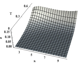
Figure 1: Energy density $u\left(n,T\right)$ given by Eq. 4.

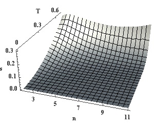
Figure 2: Helmholtz free energy density $f\left(n,T\right)=F\left(V,n,T\right)/V$ (see Eq. 6).

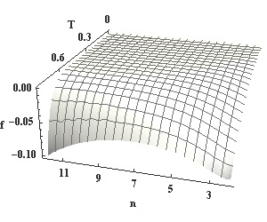
Figure 3: Entropy density $s\left(n,T\right)=S\left(V,n,T\right)/V$ (see Eq. 7).

The functions $u\left(n,T\right)$, $f\left(n,T\right)$ and $s\left(n,T\right)$ do not have a global maximum nor minimum, but for a given temperature we can find both local maxima and minima for each potential. These critical points are located in a certain range of $n$ and $T$. Outside this region the function presents a monotonic growth because of the contribution of the term $\zeta\left(n+1\right)\Gamma\left(n+1\right)$. One can analyze the first and second derivatives respect to the dimension with the aim of determining whether the maxima and minima are restricted to a certain dimensionality. For example, at constant temperature one can goes from a minor to a major dimensionality, passing from positive to negative derivatives (or vice versa). In this changes of sign of the derivatives are the maxima (or minima) of the energy density. As the temperature increases the minima and maxima get closer to each other until they reach a saddle point (see Fig. 4).

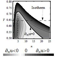
Figure 4: First derivative in the dimension for the energy density $u\left(n,T\right)$ given by Eq. 4. The vertical dashed line marks the location of the saddle point, located at $n<5$. The horizontal dashed line represents an isothermal process, in which by increasing the dimension from $n=1$ to $n=25$ the BBR system has an increasing energy density $u$ (positive derivative), then it reaches a local maximum and decreases (negative derivative) until it reaches a local minimum and then $u$ increases again.

One point is of special interest, the point at which one cannot longer obtain any of both extreme points (nor minima nor maxima). The saddle point separates the regions of maxima an minima. This is summarized in Table 1.

	$u\left(n,T\right)$	$f\left(n,T\right)$	$s\left(n,T\right)$	$h\left(n,T\right)$
Maxima in	$n\leq 4$	$n>3$	$n\leq 4$	$n\leq 4$
Minima in	$n>4$	$n\leq 3$	$n>4$	$n>4$

Table 1: Location of maxima and minima of energy, Helmholtz free energy, entropy and enthalpy densities are restricted to certain dimensionalities.

If a hypersphere is considered as the black body system, the total potential can be found. The volume of this hypersphere of radius $R$ is given by the expression [34],

$$V=\frac{\pi^{\frac{n}{2}}}{\Gamma\left(\frac{1}{2}n+1\right)}R^{n}.$$

In Figs. 5-7 the thermodynamic potentials $U\left(n,T.R\right)$, $F\left(n,T,R\right)$, and $S\left(n,T,R\right)$ are shown (see Eqs. 3, 6, and 7 respectively),

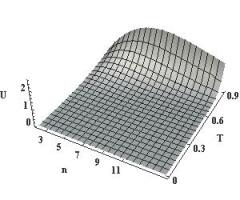
Figure 5: Energy $U\left(n,T,R=.9\right)$ given by Eq. 3.

In these cases we cannot find any restriction in the dimensionality at which the maxima or minima would appear. The variables $R$, $T$, and $n$ can be combined in several ways in order to produce critical points at any dimension.

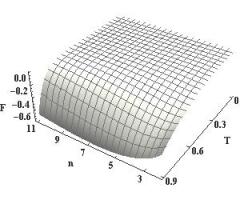
Figure 6: Helmholtz free energy $F\left(n,T,R=.9\right)$ given by Eq. 6.

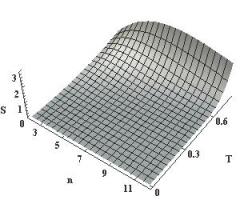
Figure 7: Entropy $S\left(n,T,R=.9\right)$ given by Eq. 7.

VIII. A possible simple application to cosmology.

Since the works by Kaluza and Klein [7, 8], many proposals about universe’s models with dimensionality different from three have been published [7, 8, 17, 18, 20, 21, 31, 32, 33, 40, 41, 42]. Remarkably this has been the case for papers stemming from the string, d-branes and gauge theories [10, 11, 12, 15, 20]. However, nowadays we only have evidence for a universe with three space and one time dimensions. In the present section we make a simple thermodynamic analysis leading to a scenario of a universe with only 3 space dimensions. This scenario is present within the region of high temperatures and low dimensionality mentioned in the previous section.

Temperatures as high as $10^{32}K$ are only possible in a very primeval time in the evolution of the universe. It is known that the period dominated by radiation is from $t=10^{-44}s$ to $t\approx 10^{10}s$ [43], that means, that in this period the universe could have been well described by a spatially flat, radiation-only model [44]. Thus, considering the whole primeval universe as a black body system in an Euclidean space is in principle a reasonable approach.

In some textbooks [45, 46] it is referred that the critical energy density at the time of $t\approx 1t_{P}$ was about $u\approx 1E_{P}/V_{P}$ ($V_{P}$ is a Planck volume) and the temperature approximately $T\approx 1T_{P}$ . The energy density and temperature obtained when the maximum of the energy density is located at $n=3$ (see Fig 2) are surprisingly near of the values above referred.

According to string theories at some point (at the end of the Planck epoch) the rest of the dimensions collapsed and only the known 3-dimensional space grew bigger. The remaining question is: why do we live in a $3-d$ universe?

Let’s suppose that by some sort of mechanism the dimension of space was reduced from a given initial value of the dimension to a final state with $n=3$. In this scenario a change of energy can be obtained as it is shown in Table 2.

$n$	$u\;\left[E_{p}/V_{P}\right]$	$E$$\;[GeV/V_{P}]$
3	0.49	6.02E18
4	0.66	8.04E18
9	2.74	3.34E19
25	15000	1.83E23

Table 2: Energy (Eq. 4) at $T=0.93T_{p}$ within a Planck volume. $T=0.93T_{p}$ is an arbitrary value close to $T_{P}$.

If such transitions would occur between an initial and a final dimension, a difference of energy could exist. In some cases the “missing” energy represents a significant part of the total initial energy, as can be seen in Table 3.

$n_{initial}$	$n_{final}$	$\Delta E_{p}$	$\%E_{missing}$
4	3	0.16	25.177
9	3	2.24	82
10	3	3.42	87.42
25	3	14999.7	99.9967

Table 3: Change of energy at the temperature of $T=0.93T_{p}$ in a Planck volume.

The energy difference between an initial and the final state is quite big, in each case bigger than the total energy density for $n=3$, and certainly must be taken into account whenever this model could be applied in such processes. In that case, the questions of where did that energy go? and if could it be in the extra compactified dimensions? may be relevant. For example, for a $9+1$ space-time, the $6$ extra spatial dimensions are supposed to be compactified, with a compactification related to the Planck scale [31]. One can look at those numbers and think in a different way: the universe should have been $1.34$ times more energetic to form a $4$ dimensional space, $5.6$ times more energetic for a $9$ dimensional space and $30476$ times more energetic to form a $25$ dimensional space. Except for $n=4$ the difference between any scenario is considerable.

In the previous section we saw that the maxima and minima are restricted to certain dimensionality, thus it could be a worthy effort to explore whether some thermodynamic property could intervene in the construction of a $3-$dimensional universe.

It is possible from this generalization of the Planck function to an Euclidean $n-$dimension space, to incorporate some corrections. Given the range of high temperatures, a modification of the dispersion relation found in LQG can be considered.

IX. LQG corrections

There is a large number of people in the scientific community that accept the possibility of the existence of extra dimensions beside the $3+1$ known space-time dimensions. If one is willing to give the black body radiation a cosmological context, it is necessary to ask about the applicability of the above ideas in the regime of very high energies and temperatures. Nowadays, it is clear the necessity of having a theory that unifies the quantum world with the general relativity in order to understand better the possible scenarios of the high energy and the physics near the Planck epoch. One path to do this is by the modification of general relativity, that is quantum gravity, and this is the scope given by some important research programs. In the context of brane theories it is possible to modify the geometrical part of the Einstein equations to incorporate extra dimensions, which have had certain success in explaining the dark energy problem and the interpretations of astronomical data [30]. On the other hand, the extra dimensions are considered to have the size of the Planck scale and remain in certain way hidden to our detectors [10, 11, 12, 15]. In a variety of quantum gravity treatments, string theory, LQG, doubly special relativity, models based in non commutative geometry, there exists a common topic: the dispersion relation modification. Some of these are related to address black hole thermodynamic problems. Nozari and Anvari in Ref. [30] proposed a modification of the Planck law. This was made by using a modified dispersion relation showed in [30, 47, 48], in which the square of the energy-momentum vector is

$$\vec{p}^{2}\simeq E^{2}-\mu^{2}+\alpha L_{P}^{2}E^{4}+\alpha^{\prime}L_{P}^{4}E^{6}+\mathcal{O}\left(L_{P}^{6}E^{8}\right),$$ (16)

where $L_{P}$ is the Planck length and it depends on the dimensionality of the space-time [48], $E$ is the energy and $\alpha$ and $\alpha^{\prime}$ take different values depending on the details of the quantum gravity candidates. Finally the modified spectral energy density showed in [30] is,

$$g\left(\nu\right)\nu d\nu=\frac{2\pi^{\frac{n}{2}}\left(n-1\right)\nu^{n}}{\Gamma\left(\frac{n}{2}\right)\left(e^{\nu/T}-1\right)}\{1+\left(\frac{3}{2}+\frac{n-1}{2}\right)\alpha\nu^{2}$$

$$+\left[\alpha^{2}\left(-\frac{5}{8}+\frac{3\left(n-1\right)}{4}\right)+\alpha^{\prime}\left(\frac{5}{2}+\frac{n-1}{2}\right)\right]\nu^{4}\}$$ (17)

In this way, the internal energy density is given by the following expression (see [30]),

$$u\left(n,T\right)=\frac{2\pi^{\frac{n}{2}}\left(n-1\right)T^{n+1}}{\Gamma\left(\frac{n}{2}\right)}\{\Gamma\left(n+1\right)\zeta\left(n+1\right)+$$

$$\left(\frac{3}{2}+\frac{n-1}{2}\right)\alpha T^{2}\Gamma\left(n+3\right)\zeta\left(n+3\right)+$$

$$\left[\alpha^{2}\left(-\frac{5}{8}+\frac{3\left(n-1\right)}{4}\right)+\alpha^{\prime}\left(\frac{5}{2}+\frac{n-1}{2}\right)\right]\times$$

$$T^{4}\Gamma\left(n+5\right)\zeta\left(n+5\right)\}.$$ (18)

and from Eq. (5) and Appendix A, the Helmholtz free energy density now is,

$$f\left(n,T\right)=-\frac{2\pi^{\frac{n}{2}}\left(n-1\right)T^{n+1}}{\Gamma\left(\frac{n}{2}\right)}\{\frac{\Gamma\left(n+1\right)\zeta\left(n+1\right)}{n}+$$

$$\frac{\left(\frac{3}{2}+\frac{n-1}{2}\right)\alpha T^{2}\Gamma\left(n+3\right)\zeta\left(n+3\right)}{n+2}$$

$$+\left[\alpha^{2}\left(-\frac{5}{8}+\frac{3\left(n-1\right)}{4}\right)+\alpha^{\prime}\left(\frac{5}{2}+\frac{n-1}{2}\right)\right]\times$$

$$\frac{T^{4}\Gamma\left(n+5\right)\zeta\left(n+5\right)}{n+4}\}.$$ (19)

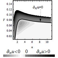
Figure 8: First derivative in the dimension for the energy density $u\left(n,T\right)$ given by Eq. 18. The values of $\alpha=0.1$ and $\alpha^{\prime}=2.28$ are such that the curves showed in [30] are reproduced.

One relevant aspect is that it is possible to get the same interesting behavior of the thermodynamic potential densities mentioned before, but one order of magnitude smaller in the temperature than in the model with no LQG modifications, as can be seen in Fig. 8 (see Fig. 4 for comparison).

X Conclusions

It has been presented the generalizations of the entropy, free energies of Helmholtz and Gibbs, enthalpy, pressure, the equation for adiabatic processes, the Carnot cycle efficiency, and the chemical potential for the black body radiation in an $n$-dimensional Euclidean space.

This flat space generalization with reasonable suppositions could be a good approximation to model the very early universe. The peculiar behavior of the thermodynamic potential densities in the region of low dimensionality-high temperature could be profoundly linked with the 3-dimensional character of our space since the beginning of time. In particular, the maximization of some thermodynamic functions seems a suitable scenario to choose $n=3$ since the very early universe. Finally, a correction that takes into account modifications to the dispersion relations stemming from loop quantum gravity are incorporated into the analysis.

Appendix A

Riemann’s zeta function $$\zeta\left(x\right)=\frac{1}{1^{x}}+\frac{1}{2^{x}}+\frac{1}{3^{x}}+...$$ $$\zeta\left(x\right)=\frac{1}{\Gamma\left(x\right)}\intop_{0}^{\infty}\frac{u^{x-1}}{e^{u}-1}du\;\;\;\;\;\;\;x>1.$$ (20)

Integrating $\quad\intop_{\chi=0}^{\infty}\chi^{n-1}ln\left(1-e^{-\chi}\right)d\chi$ by parts.

$$u=ln\left(1-e^{-\chi}\right),\;\;\;du=\frac{e^{-\chi}}{1-e^{-\chi}}d\chi=\frac{1}{e^{\chi}-1}d\chi$$

$$dv=\frac{1}{n}d\chi^{n},\;\;\;\;\;\;\;\;\;\;\;\;v=\frac{\chi^{n}}{n}\;\;\;\;\;\;\;\;\;\;\;\;\;\;\;\;\;\;\;\;\;\;\;\;$$

$$\intop_{\chi=0}^{\infty}\chi^{n-1}ln\left(1-e^{-\chi}\right)d\chi=\frac{\chi^{n}}{n}ln\left(1-e^{-\chi}\right)\mid_{\chi=0}^{\infty}$$

$$-\frac{1}{n}\intop_{\chi=0}^{\infty}\frac{\chi^{n}}{e^{\chi}-1}d\chi.$$

The first member of the right side of the equation, by L’Hopital’s rule is zero

$$\underset{\chi\rightarrow 0}{lim}\frac{ln\left(1-e^{-\chi}\right)}{\chi^{-n}}=\underset{\chi\rightarrow 0}{lim}-\frac{\chi^{n+1}}{n\left(e^{\chi}-1\right)}$$

$$=\underset{\chi\rightarrow 0}{lim}-\frac{\left(n+1\right)\chi^{n}}{ne^{\chi}}=0,$$

$$\underset{\chi\rightarrow\infty}{lim}\frac{ln\left(1-e^{-\chi}\right)}{\chi^{-n}}=\underset{\chi\rightarrow\infty}{lim}-\frac{\chi^{n+1}}{n\left(e^{\chi}-1\right)}$$

$$=\underset{\chi\rightarrow\infty}{lim}-\frac{\left(n+1\right)\chi^{n}}{ne^{\chi}}=...=\underset{\chi\rightarrow\infty}{lim}-\frac{\left(n+1\right)!}{n^{2}e^{\chi}}=0.$$

And because of Eq.(20)

$$\intop_{\chi=0}^{\infty}\chi^{n-1}ln\left(1-e^{-\chi}\right)d\chi=-\frac{1}{n}\zeta\left(n+1\right)\Gamma\left(n+1\right).$$

Appendix B. Carnot efficiency

From the fist law of thermodynamics

$$dQ=dU+pdV=npdV+nVdp+pdV$$

because $p=p\left(T\right),$in an isothermal path $p=const$ and $dp=0$,

$$dQ=(n+1)pdV$$

$$Q_{1}=(n+1)\intop_{1}^{2}p_{1}dV=(n+1)p_{1}\intop_{1}^{2}dV=(n+1)p_{1}(V_{2}-V_{1})$$ (21)

and

$$Q_{2}=(n+1)p_{3}\intop_{3}^{4}dV=(n+1)p_{3}(V_{4}-V_{3})$$ (22)

$$\Rightarrow\eta=1-\frac{p_{3}(V_{3}-V_{4})}{p_{1}(V_{2}-V_{1})},$$ (23)

$$\eta=1-\frac{p_{3}(V_{3}-V_{4})}{p_{1}(V_{2}-V_{1})},$$

from Eq. (15)

$$p_{1}V_{1}^{\frac{n+1}{n}}=p_{3}V_{4}^{\frac{n+1}{n}}\qquad y\qquad p_{1}V_{2}^{\frac{n+1}{n}}=p_{3}V_{3}^{\frac{n+1}{n}},$$

then

$$V_{1}p_{1}^{\frac{n}{n+1}}=V_{4}p_{3}^{\frac{n}{n+1}}\qquad y\qquad V_{2}p_{1}^{\frac{n}{n+1}}=V_{3}p_{3}^{\frac{n}{n+1}},$$

$$p_{1}^{\frac{n}{n+1}}(V_{2}-V_{1})=p_{3}^{\frac{n}{n+1}}(V_{3}-V_{4}),$$

$$\frac{(V_{3}-V_{4})}{(V_{2}-V_{1})}=\frac{p_{1}^{\frac{n}{n+1}}}{p_{3}^{\frac{n}{n+1}}},$$

taking a look to Eq. (23) and because $p_{2}=p_{3}$,

$$\eta_{c}=1-\frac{p_{1}^{\frac{n}{n+1}}p_{2}}{p_{2}^{\frac{n}{n+1}}p_{1}}=1-\frac{p_{2}^{\frac{1}{n+1}}}{p_{1}^{\frac{1}{n+1}}}$$

we know that,

$$p=a_{n}T^{n+1}$$

$$\Rightarrow p^{\frac{1}{n+1}}=\alpha T,$$

finally arriving to the desired expression for the Carnot efficiency,

$$\eta_{c}=1-\frac{T_{2}}{T_{1}}.$$

Acknowledgement.

We want to thank partial support from COFAA-SIP-EDI-IPN and SNI-CONACYT, MÉXICO.

References

- [1] C. Tolman, Richard 1934 Relativity, Thermodynamics and Cosmology (Dover, new York)
- [2] W. Kolb, Edward and S. Turner, Michael 1994 The Early Universe (Westview Press, New York)
- [3] Weinberg, Steven 2008 Cosmology (Oxford University Press, Oxford)
- [4] Einstein A 1907 Über das Relativitätsprinzip und die aus demselben gezogene Folgerungen (On the Relativity Principle and Conclusions Drawn from It) Jahrbuch der Radioaktivität und Elektronik 4 (411)
- [5] Planck M 1908 Ann. Phys. (Lpz) 26 1
- [6] Brandenberger Robert and Vafa C 1989 Superstrings in the early universe. Nucl. Phys. B 316, 391-410
- [7] Kaluza Theodor 1921 Zum Unitätsproblem in der Physik”. Sitzungsberichte Preussische Akademie der Wissenschaften (Math. Phys.) 966–972
- [8] Klein Oskar 1926 Quantentheorie und fünfdimensionale Relativitätstheorie, Zeitschrift für Physik a Hadrons and Nuclei 37 (12), 895–906
- [9] J D Barrow and W S Hawthorne 1990 Equilibrium matter fields in the early universe Mon. Not. R. astr. Soc 243, 608-609.
- [10] Arkani-Hamed N, Dimopoulos S, and Dvali G R 1998 The hierarchy problem and new dimensions at a millimeter Phys. Lett. B 429, 263–272; Antoniadis I, Arkani-Hamed N, Dimopoulos S and Dvali G 1998 New dimensions at a millimeter to a fermi and superstrings at a TeV Phys. Lett. B 436, 257-263
- [11] Randall L and Sundrum R 1999 Large Mass Hierarchy from a Small Extra Dimension Phys. Rev. Lett 83, 3370; Randall L and Sundrum R 1999 An Alternative to Compactification Phys. Rev. Lett 83, 4690
- [12] Dvali G, Gabadadze G and Porrati M 2000 Metastable Gravitons and Infinite Volume Extra Dimensions Phys. Lett. B 484, 112-118
- [13] Barton Zwiebach 2004 A first course in string theory (Cambridge University Press, New York)
- [14] Erdmenger Johanna 2009 String Cosmology, Modern String Theory Concepts from the Big Bang to Cosmic Structure (Wiley-VCH, Germany)
- [15] Cordero Rubén and Rojas Efraín 2011 Classical and quantum aspects of braneworld cosmology AIP Conference Proceedings, 1396, 55
- [16] R Brandenberger 2011 Introduction to Early Universe Cosmology. arXiv:1103.2271 [astro-ph.CO]
- [17] Jonas Mureika and Dejan Stojkovic. “Detecting Vanishing Dimensions via Primordial Gravitational Wave Astronomy”. Phys.Rev.Lett. 106, (2011) 101101.
- [18] Landsberg P T and De Vos A 1989 The Stefan Boltzman constant in an n-dimensional space J. Phys. A: Mathematics and General, 22, 1073-1084
- [19] Pereira S H 2001 On the Sakur Tetrode equation of state in an expanding universe Revista Mexicana de Física E57(1) 11-15
- [20] García-Compeán Hugo and Loaiza-Brito Oscar 2000 Lectures on Strings, D-branes and Gauge Theories arXiv:hep-th/0003019v1
- [21] Menon V J and Agrawal D C 1998 Comment on “The Stefan-Boltzmann constant in -dimensional space” J. Phys. A: Math. Gen. 31, 1109-1110
- [22] J D Barrow. ”Dimensionality”. Phil. Trans. Roy. Soc. A 310, 337-346 (1983).
- [23] Craig Callender, “Answers in search of a question: “proofs” of the tri-dimensionality of space”. Studies in History and Philosofy of Modern Physics, 36, (2005) 113-136.
- [24] P Ehrenfest, “In what way does it become manifest in the fundamental laws of physics that space has three dimensions?”. Proceeding of the Amsterdam Academy, 20, (1917) 200-209.
- [25] Max Tegmark, “On the dimensionality of spacetime”. Class. Quantum Grav., 14, (1997) L69-L75.
- [26] J D Barrow & F J Tipler, The Anthropic Cosmological Principle (OUP, 1986),pp 258-76.
- [27] Steven Weinstein, “Multiple Time Dimensions”. arXiv:0812.3869v1 (2008)
- [28] R Brandenberger. “Introduction to Early Universe Cosmology”. arXiv:1103.2271 [astro-ph.CO] (2011)
- [29] Silvia De Bianchi and J D Wells, “Explanation and dimensionality of space. Kant’s argument revisited”. Synthese, 192 (2015) 287-303.
- [30] Nozari Kourosh and Anvari S F 2012 Black body radiation in a model universe with large extra dimensions and quantum gravity effects arXiv:1206.5631v1
- [31] Ramos Ramaton and Boschi-Filho Henrique 2009 Blackbody radiation with compact and non-compact extra dimensions arXiv:0910.1561v1 [quant-ph]
- [32] Cardoso Tatiana R and S de Castro Antonio 2005 The blackbody radiation in a D-dimensional universes Rev. Bras. Ensino Fís. vol.27 no.4 Sao Paulo
- [33] Alnes Haavard, Ravndal Finn and Wehus Ingunn Kathrine 2005 Black-body radiation in extra dimensions arXiv:quant-ph/0506131v1
- [34] Greiner Walter, Neise Ludwig and Stöcker Horst 1995 Thermodynamics and Statistical Mechanics (Springer, E.U.A, pp 130-131)
- [35] Ares de Parga G, López-Carrera B and Angulo-Brown F 2005 A proposal for relativistic transformations in thermodynamics J. Phys. A: Math. Gen. 38, 2821-2834
- [36] Ares de Parga G, López-Carrera B 2009 Redeffined relativistic thermodynamics based on the Nakamura formalism Physica A 388, 4345-4350
- [37] López-Carrera B, Granados V and Ares de Parga G 2008 An alternative deduction of relativistic transformations in thermodynamics Revista Mexicana de Física 54(1), 15-19
- [38] Julian Gonzalez-Ayala and F Angulo-Brown 2013 The universality of the Carnot theorem Eur. J. Phys. 34, 273–289
- [39] http://physics.nist.gov/cgi-bin/cuu/Category?view=gif&Universal.x=88& Universal.y=11
- [40] Padmanabhan T 2003 Cosmological Constant. The Weight of the Vacuum Physics Reports 380, 235-320
- [41] Dejan Stojkovic 2013 Vanishing dimensions: A review Mod.Phys.Lett. A28, 1330034
- [42] Niayesh Afshordi, Dejan Stojkovic. ”Emergent Spacetime in Stochastically Evolving Dimensions”. Phys.Lett. B739, (2014) 117-124.
- [43] Cepa Jordi 2007 Cosmología Física”. (Ed. Akal, Madrid España)(In Spanish)
- [44] Ryden Barbara 2006 Introduction to Cosmology (Addison Wesley, Ohio USA)
- [45] Liddle Andrew 2004 An Introduction to Modern Cosmology (Wiley, Great Britain)
- [46] Maroto L Antonio and Ramirez Juan 2004 A Conceptual Tour About the Standard Cosmological Model arXiv:astro-ph/0409280v1
- [47] Amelino-Camelia G, Arzano M and Procaccini A 2004 Severe constraints on Loop-Quantum-Gravity energy-momentum dispersion relation from black-hole area-entropy law Phys. Rev. D 70, 107501; Amelino-Camelia G, Arzano M, Ling Y and Mandanici G 2006 Black-hole thermodynamics with modified dispersion relations and generalized uncertainty principles Class. Quant. Grav. 23, 2585
- [48] Sefiedgar A S and Sepangi H R 2010 General Relativity and Quantum Cosmology Phys. Lett. B 692, 281; Sefiedgar A S, Nozari K and Sepangi H R 2011 Modified dispersion relations in extra dimensions Phys. Lett. B 696, 119; Sefiedgar A S and Sepangi H R 2012 General Relativity and Quantum Cosmology Phys. Lett. B 706, 431