Where are the roots of the Bethe Ansatz equations?

Abstract

Changing the variables in the Bethe Ansatz Equations (bae) for the xxz six-vertex model we had obtained a coupled system of polynomial equations. This provided a direct link between the bae deduced from the Algebraic Bethe Ansatz (aba) and the bae arising from the Coordinate Bethe Ansatz (cba). For two magnon states this polynomial system could be decoupled and the solutions given in terms of the roots of some self-inversive polynomials. From theorems concerning the distribution of the roots of self-inversive polynomials we made a thorough analysis of the two magnon states, which allowed us to find the location and multiplicity of the Bethe roots in the complex plane, to discuss the completeness and singularities of Bethe’s equations, the ill-founded string-hypothesis concerning the location of their roots, as well as to find an interesting connection between the bae with Salem’s polynomials.

Exactly integrable models provide benchmarks for different areas of physics as statistical mechanics baxter1 , condensed matter physics essler , quantum field theory abdalla , nuclear physics nuclear , atomic-molecular physics angela and more recently for high energy physics through the gauge theory, string theory and super-Yang-Mills theories zarembo . An important tool is the algebraic Bethe Ansatz takhfadd culminating in the Bethe Ansatz equations bethe ; lieb . Yet analytic results have been unable to scale the unsurmountable wall of find their roots: these have treated mostly by numerical methods, which are in general hard to implement.

Here we analyze the solutions of the Bethe equations using some theorems regarding self-inversive polynomials in order to answer the question made in the title.

The ba equations for the xxz six-vertex model on a $L\times L$ lattice, as deduced from the aba are

$$\left(\frac{\sinh(\lambda_{i}+\eta)}{\sinh\lambda_{i}}\right)^{L} = \prod_{k\neq i}^{N}\frac{\sinh(\lambda_{i}-\lambda_{k}+\eta)}{\sinh(\lambda_{i}-\lambda_{k}-\eta)},$$

$$i = 1,2,...,N.$$ (1)

The solutions $\left\{\lambda_{1},\lambda_{2},...,\lambda_{N}\right\}$ of (1) will furnish all $2^{L}$ states of the transfer matrix for a lattice of $L$ columns.

Multiplying side-by-side these equations we get

$$\prod_{i=1}^{N}\left(\frac{\sinh(\lambda_{i}+\eta)}{\sinh\lambda_{i}}\right)^{L}=1,$$ (2)

which suggests the following changing of variables,

$$\frac{\sinh(\lambda_{i}+\eta)}{\sinh\lambda_{i}}=c_{i},\quad i=1,2,...,N,$$ (3)

so that the $c_{i}$ should be subject to the constraint equation

$$c_{1}^{L}c_{2}^{L}\cdots c_{N}^{L}=1,$$ (4)

which reflects the translational invariance of the periodic lattice.

Now, Eq. (3) can be easily solved for the rapidities $\lambda_{i}$,

$$\lambda_{i}=\mbox{arctanh}\left(\frac{\sinh\eta}{c_{i}-\cosh\eta}\right)=\frac{1}{2}\ln\left(\frac{c_{i}-\mathrm{e}^{-\eta}}{c_{i}-\mathrm{e}^{\eta}}\right),$$ (5)

where the functions $\mbox{arctanh}(z)$ and $\ln(z)$ must be regarded as multivalued complex functions, each branch differing by multiples of $i\pi$. The new variables $c_{i}$ should yet to be determined. To this end we insert (5) back on (1), which gives us a system of $N$ polynomial equations,

$$c_{i}^{L} = (-1)^{N-1}\prod_{k\neq i}^{N}\frac{c_{i}c_{k}-2\Delta c_{i}+1}{c_{i}c_{k}-2\Delta c_{k}+1},$$

$$\Delta = \cosh\eta,\quad i=1,2,..,N.$$ (6)

Here we observe that writing $c_{i}=\exp(k_{i})$, where $k_{i}$ are the Bethe’s momenta, leaves (6) exactly equal to the bae derived in the cba for the xxz six-vertex model lieb . Therefore, the relations (5) establish a direct link between the Bethe states of the aba and the Bethe wave-functions of the cba. Thus, all the results about completeness, singularities etc. which are valid for cba, as obtained by Baxter in baxter , will be also valid for the algebraic version.

For $N=1$ the equations (6) reduce to $c_{1}^{L}=1$ and $c_{1}$ is one of the $L$ roots of unity. This means that in a periodic lattice of $L$ columns, the free pseudo-particle (magnon) has $L$ different rapidities given by the Bethe roots (5).

For $N=2$ we have three coupled equations for $c_{1}$ and $c_{2}$,

$$c_{1}^{L}\left(c_{1}c_{2}-2\Delta c_{2}+1\right)+c_{1}c_{2}-2\Delta c_{1}+1 = 0,$$

$$c_{2}^{L}\left(c_{1}c_{2}-2\Delta c_{1}+1\right)+c_{1}c_{2}-2\Delta c_{2}+1 = 0,$$

$$c_{1}^{L}c_{2}^{L} = 1.$$ (7)

From the constraint equation we can set $c_{2}=\omega_{a}/c_{1}$ and the system becomes reduced to

$$P_{a}(c_{1})=0,\qquad P_{a}(c_{1})/c_{1}^{L}=0,$$ (8)

where $P_{a}(c_{1})$ are the following $L$-degree polynomials,

$$P_{a}(c_{1}) = (1+\omega_{a})c_{1}^{L}-2\Delta\omega_{a}c_{1}^{L-1}-2\Delta c_{1}+(1+\omega_{a}),$$

$$\omega_{a} = \mathrm{e}^{\frac{2i\pi}{L}a},\qquad a=1,2,...,L.$$ (9)

Notice that $P_{a}(c_{1})$ satisfies $P_{a}(c_{1})=c_{1}^{L}P_{a}(\omega_{a}/c_{1})$, the pair $\left(c_{1},c_{2}\right)$ and $\left(c_{2},c_{1}\right)$ therefore representing the same solution of (7). Moreover $P_{a}(c_{1})$ is a self-inversive polynomial since they satisfy $P_{a}(c_{1})=\omega_{a}c_{1}^{L}\overline{P}_{a}(1/c_{1})$, where the bar means complex-conjugation.

It seems that explicit solutions (in terms of radicals) of the equation $P_{a}(c_{1})=0$ can be written only for small values of $L$, or for very special values of $a$ and $\Delta$. The roots of $P_{a}(c_{1})$ of course can be easily obtained numerically. It is the self-inversive property of the polynomials $P_{a}(c_{1})$ that provides crucial informations about the location of the Bethe roots.

We know from the theory of self-inversive polynomials marden that their roots are all symmetric with respect to the complex unit circle $U=\{z\in C:|z|=1\}$. For the polynomials $P_{a}(c_{1})$, however, we get a better scenario, since their roots can be distributed only into two ways, namely, either they are all on $U$ or only two dual roots $s$ and $\omega_{a}/s$ are not on $U$. In fact, the exact behavior of the roots depends on the values of $\Delta$ from which two are critical,

$$\Delta_{1}=\left|\frac{1+\omega_{a}}{2}\right|\quad\mathrm{and}\quad\Delta_{2}=\frac{L}{L-2}\left|\frac{1+\omega_{a}}{2}\right|.$$ (10)

and this behavior can be summarized as follows,

i) If $|\Delta|<\Delta_{1}$ then all roots of $P_{a}(c_{1})$ are on $U$ and they are simple;

ii) If $|\Delta|>\Delta_{2}$ then only two dual roots of $P_{a}(c_{1})$ are out $U$ and all roots are simple;

iii) If $|\Delta|=\Delta_{1}$ then all roots of $P_{a}(c_{1})$ are on $U$ but two roots on $U$ can be coincident;

iv) If $|\Delta|=\Delta_{2}$ then two roots of $P_{a}(c_{1})$ are out $U$ but three roots on $U$ can be coincident;

v) If $\Delta_{1}<|\Delta|<\Delta_{2}$ The roots are distributed as in i) or ii), depending on the values of $L$ and $a$.

The proof of the statements i) and ii) can be obtained from theorems presented by Vieira in ricardo , which are generalizations of theorems presented previously by Lakatos and Losonczi in poly1 ; iii) and iv) can be verified directly from the factorization of $P_{a}(c_{1})$ and v) was verified numerically only (since the theorems mentioned above does not hold in this case). The exact behavior in the case v) is the following: all roots of $P_{a}(c_{1})$ will be in $U$ if, for even $L$, $a$ is odd and for odd $L$, if $a$ is odd and $a<(L-1)/2$ or when $a$ is even and $a>(L+1)/2$; for $a=(L-1)/2$ or $a=(L+1)/2$ the roots are all in $U$ if $L\equiv 3\,(\text{mod }4)$; otherwise the roots are in $U$, except for two dual roots $s$ and $\omega_{a}/s$.

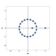
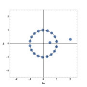
Figure 1: Roots of $P_{L}(c_{1})$ and $P_{1}(c_{1})$ for $L=20$ and $\Delta=2$. The first figure shows that $P_{L}(c_{1})$ is a Salem’s polynomial. In the second figure we have $P_{1}(c_{1})$ behaves as a “rotated” Salem’s polynomial.

Notice that in the case in the case i), where the roots of $P_{a}(c_{1})$ are all in $U$, if the coefficients of $P_{a}(c_{1})$ are integers then follows from a celebrated theorem of Kronecker Smith that all roots of $P_{a}(c_{1})$ are indeed roots of unit and therefore they can be expressed by radicals. Moreover, in ii) the polynomials $P_{a}(c_{1})$ have only two dual roots out of $U$. In algebraic number theory a polynomial (with integer coefficients) whose roots are all on the complex unit circle except for two positive reciprocal roots $r$ and $1/r$ is named a Salem polynomial. Therefore the polynomials $P_{L}(c_{1})$ are Salem’s polynomials when $\Delta$ is a positive integer greater than $1$. See Fig. 1, 2 and 3. This is an interesting and non expected relation between the bae for the two magnon state and Salem’s polynomials, since they are found only in a few fields of mathematical physics, for instance, in Coxeter systems and the $(-2,3,7)$-pretzel knot theory salem .

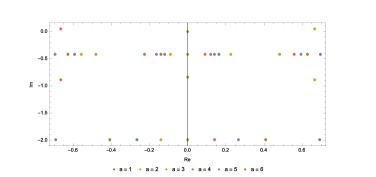
Figure 4: Bethe’s Roots for $L=6$ and $\Delta=2/3$. Notice that the roots of $P_{a}(c_{1})$ which lie on $U$ are mapped on the lines $y=-|\eta|/2$ and $y=-|\eta+i\pi|/2$. This leads to 1-string solutions. The dual roots of $P_{a}(c_{1})$ which are out of $U$ are led to pairs with the same real part, so they are related to 2-string solutions.

The analysis above gives us the distribution of the roots of $P_{a}(c_{1})$. The correspondent location of the Bethe roots $\lambda_{i}$ is provided by the formula (5), which can be seen as a conformal mapping from the complex variables $c_{i}$ to $\lambda_{i}$. In fact, if $|\Delta|>1$, so that $\eta$ is real, this mapping will send the complex unit circle $U$ into the vertical line $x=-|\eta|/2$. On the other hand, if $|\Delta|<1$ then (5) will map $U$ into a horizontal lines $y=-|\eta|/2$ and $y=-|\eta+i\pi|/2$. Notice that usually the Bethe roots are expected to be arranged (in the thermodynamical limit $L\gg 1$) into groups of the same real part called strings viola1 . A $n$-length string is a group of $n$ Bethe roots all of them with the same real part. From what was said above we can see that, for $|\Delta|<1$, the roots of $P_{a}(c_{1})$ which lie on $U$ will lead to 1-string solutions, while the two dual roots outside $U$ will lead to 2-string solutions. The same will be true for the case $|\Delta|>1$ provided we redefine a $n$-length string as group of $n$ Bethe roots all of them with the same imaginary part. See Fig. 4 and 5. Notice as well that several violations of the string hypothesis were already reported viola1 . This not happens in our approach, since the string hypothesis is not used in our deduction.

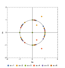
Figure 2: The roots of $P_{a}(c_{1})$ for $L=6$ and $\Delta=2/3$. For $a=\{1,5,6\}$ we have $|\Delta|<\Delta_{1}$, so the roots are all in $U$. For $a=\{2,4\}$ we have $\Delta_{1}<|\Delta|<\Delta_{2}$ and since $a$ is even we have in each case two dual roots out of $U$. For $a=3$ we have $|\Delta|>\Delta_{2}$, then two roots are also out of $U$ (these roots are $0$, and $-\infty$).

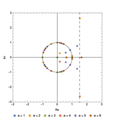
Figure 3: The roots of $P_{a}(c_{1})$ for $L=6$ and $\Delta=3/2$. For all values of $a$ we have $|\Delta|\geq\Delta_{2}$ (the equality occurs only for $P_{6}(c_{1})$, which does not have three roots coincident). Therefore all $P_{a}(c_{1})$ have two dual roots out of $U$.

Here we remark the importance of this analysis for the range of $\Delta$ in the study of the completeness of the Bethe states and in the string hypothesis.

Let us first to consider $|\Delta|\neq\Delta_{1}$ and $|\Delta|\neq\Delta_{2}$. For odd $L$ we have that $P_{a}(c_{1})$ factors to $P_{a}(c_{1})=(c_{1}+\omega_{b})Q_{a}(c_{1})$, where $Q_{a}(c_{1})$ are $L$ self-inversive polynomials of $L-1$ degree and $2b\equiv a\text{ (mod }L)$. However, the solutions $c_{1}=-\omega_{b}$ lead us to $\lambda_{1}=\lambda_{2}$, that is, to $L$ states not belonging to the two magnon sector. Hence, the wanted solutions are the $L-1$ roots of each polynomial $Q_{a}(c_{1})$. A half of these solutions are related by permutations, so we get the exact number of solutions for the two magnon sector for odd $L$, namely, $L(L-1)/2$.

This same number of physical states for $L$ even $(L=2k)$ is obtained by a more elaborate sum of terms. This happens because the case $\omega_{a}=-1$ is special, since $P_{a}(c_{1})$ collapses in this case to

$$P_{L/2}(c_{1})=2\Delta c_{1}(c_{1}^{L-2}-1).$$ (11)

The possibility $c_{1}=0$ leads to $c_{2}=-\infty$ and the system (8) is not actually satisfied. However, this would lead to the finite Bethe roots $\left(\lambda_{1},\lambda_{2}\right)=\left(-\eta,0\right)$ which is in fact a solution of the Bethe equations. The explanation is that we had implicitly assumed $c_{j}\neq 0$, $1\leq j\leq L$, in deriving (3) and thus these cases must be analyzed separately. Thanks to the conjugation property, we have as well the solution $\left(\lambda_{1},\lambda_{2}\right)=\left(0,-\eta\right)$, so we get two additional solutions of the bae which must be taken into account.

For the other case, $c_{1}$ must be a $(L-2)$-root of unity and we get

$$\lambda_{1}=\frac{1}{2}\ln\left(\frac{\zeta_{j}-\mathrm{e}^{-\eta}}{\zeta_{j}-\mathrm{e}^{\eta}}\right),\quad\lambda_{2}=\frac{1}{2}\ln\left(\frac{\zeta_{j}\mathrm{e}^{-\eta}+1}{\zeta_{j}\mathrm{e}^{\eta}+1}\right),$$ (12)

where $\zeta_{j}=e^{\frac{2\pi i}{L-2}j}$, for $j=1,2,...L-2$. In this case we have $\lambda_{2}\neq\lambda_{1}$ except when $j=(k-1)/2$ or $j=3(k-1)/2$, which can only happen if $k$ is odd. Therefore, the case $a=k$ furnishes $2(k-1)$ solutions if $k$ is even, but only $2(k-2)$ solutions if $k$ is odd. Now let us consider the cases where $a\neq k$. Here follows that the equations (9) factor to $P_{a}(c_{1})=(c_{1}^{2}-\omega_{a})Q_{a}(c_{1})$ when $a$ is odd, but it not factor when $k$ is even. For even $k$ we have $k-1$ cases where $a$ is even and $k$ cases where $a$ is odd, which gives us $(k-1)\left(2k\right)+\left(k\right)\left(2k-2\right)$ solutions. For odd $k$ we have $k$ cases where $a$ is even and $k-1$ cases where $a$ is odd, which gives us $(k)\left(2k\right)+(k-1)(2k-2)$ solutions. Taking into account the solutions from $a=k$ and that half of the solutions are related by permutations we get, in both cases, a total of $k(2k-1)=L(L-1)/2$ solutions, as expected.

Here we remark that for $L=2$, $P_{1}(c_{1})$ is identically satisfied and we have a physical state with a free parameter (see baxter for more details). Moreover, it turns out that $P_{2}(c_{1})$ has only the singular solutions $c_{1}=e^{\pm\eta}$, as the solutions studied in nepo .

Now let us consider the cases where multiple roots appears. If $|\Delta|=\Delta_{1}$, here we have that, for $L=2k-1$, $(k>1$), there are $k-1$ polynomials ($a=2,4,...,k-2,k+1,k+3,...,L$) for $k$ even and $k$ polynomials ($a=2,4,...,k-1,k,k+2,k+4,...,L$) for $k$ odd which factor in the form $P_{a}(c_{1})=(1+\omega_{a})(c_{1}+\omega_{b})(c_{1}-\omega_{b})^{2}Q_{a}(c_{1})$, with $2b\equiv a\text{ (mod }L)$. For $L=2k$, $(k>1)$, $P_{a}(c_{1})$ factors as before but without double roots if $a$ is odd. It turns out that for $a$ even it now factors to $P_{a}(c_{1})=(1+\omega_{a})(c_{1}-\omega_{f})^{2}R_{a}(c_{1})$ and we have $k-1$ polynomials of this type if $k$ is even and $k$ polynomials if $k$ is odd, all with two coincident roots identified by the indices $a=2p$ and $f=p$ for $a<k$ and $f=k+p$ for $a>k$. Summarizing, the number of states for two magnon in a lattice of $L$ columns is reduced to $L(L-1)/2-\alpha$ where $\alpha=k-1$ for $k$ even and $\alpha=k$ for $k$ odd when $L=2k-1$ and $\alpha=2k-1$ when $L=2k$. A similar count holds when $|\Delta|=\Delta_{2}$. In this case however the number of states is reduced to $L(L-1)/2-\beta$ where $\beta=k$ for $k$ even and $\beta=k-1$ for $k$ odd when $L=2k-1$ and $\beta=2k$ for $k$ even and $\beta=2(k-1)$ for $k$ odd when $L=2k$.

The presence of these multiple roots in the two magnon sector mask the completeness viola1 . However, we can use the $S$-matrix language in order to understand these new states not as two magnon states, but as free bound states of two pseudo-particles with the same or parallel rapidities ($c_{1}^{L}=c_{2}^{L}=1$). This is another physical problem.

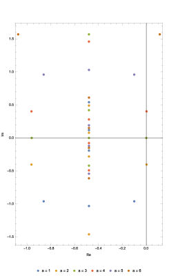
Figure 5: Bethe’s Roots for $L=6$ and $\Delta=3/2$. Now the roots of $P_{a}(c_{1})$ which lie on $U$ are mapped on the line $x=-|\eta|/2$. This leads to 1-string solutions. The dual roots of $P_{a}(c_{1})$ which are out of $U$ are led to pairs with the same imaginary parts. This leads to 2-string solutions.

Finally, a short comment about the case $N=3$. Now we have three coupled equations in $c_{1}$, $c_{2}$ and $c_{3}$ plus the constraint equation $c_{1}^{L}c_{2}^{L}c_{3}^{L}=1$. In particular, self-inversive polynomials with $\omega_{a}=\varepsilon=\pm 1$ can be obtained by setting $c_{3}=1$ and $c_{2}=\varepsilon/c_{1}$ and it has the form

$$P_{L}(c_{1}) = c_{1}^{L+1}-\left(3\varepsilon\Delta-1\right)c_{1}^{L}+\varepsilon\Delta\left(2\varepsilon\Delta-1\right)c_{1}^{L-1}$$ (13)

$$- \Delta\left(2\varepsilon\Delta-1\right)c_{1}^{2}+\left(3\varepsilon\Delta-1\right)c_{1}-\varepsilon=0.$$

In fact, we have verified that all roots of $P_{L}(c_{1})$ are in $U$ if $0\leq\Delta\leq 1$, but for other intervals we found that $P_{L}(c_{1})$ may have two or four roots out of $U$. Moreover, by removing multiple roots of these polynomials (for each value of $\varepsilon$) we got $(L-1)(L-2)/6$ states for $L\geq 6$ and taking into account the other values of $\omega_{a}$ the total is $L(L-1)(L-2)/6$ states. We will present a more detailed study of the $N\geq 3$ case in a forthcoming study. This study can be also generalized to more general vertex models as the eight-vertex model and those requiring the nested bae.

(Acknowledgments). It is ALS’s pleasure to thank professor Roland Köberle for their help and advice in preparing this article. The work of RSV has been supported by São Paulo Research Foundation (FAPESP), grant #2012/02144-7. ALS also thanks Brazilian Research Council (CNPq), grant #310625/ 2013-0 and FAPESP, grant #2011/18729-1 for financial support.

References

- (1) R. J. Baxter, Exactly solved models in statistical mechanics (Academic Press, 1982).
- (2) F. H. Essler and V. E. Korepin, Exactly solvable models of strongly correlated electrons, (World Scientific, 1994).
- (3) E. Abdalla, M.C.B. Abdalla and K. Rothe, Nonperturbative Methods in Two-Dimensional Quantum Field Theory (World Scientific, Singapore, 2001).
- (4) F. Iachello and A. Arimo, The Interacting Boson Model (Cambridge University Press, 1995).
- (5) A. Foerster and E. Ragoucy, Nucl. Phys. B, 777, 373, (2007).
- (6) J. A. Minahan and K. Zarembo, JHEP, 0303,013, (2003).
- (7) L. A. Takhtadzhan and L. D. Faddeev, Russ. Math. Surv. 34, 11, (1979).
- (8) H. Bethe, Z. Physik A 71, 205, (1931) [in The Many-Body Problem (D. C. Mattis, World Scientific, Singapore, 689, 1993)].
- (9) E. H. Lieb, Phys. Rev. 162, 162, (1967).
- (10) R. J. Baxter, J. Stat. Phys. 108, 1(2002).
- (11) Marden, M. Geometry of Polynomials. Am. Math. Soc., (Providence, 1970).
- (12) R. S. Vieira, On the number of roots of a self-inversive polynomial on the complex unit circle, (submited to publication in The Ramanujan Journal).
- (13) P. Lakatos and L. Losonczi, Publ. Math. Debrecen 65, 409, (2004).
- (14) J. McKee and C. Smyth, Number theory and polynomials, London Math. Soc. Lect. Note Series (Cambridge University Press, United Kington, 2008).
- (15) M. J. Bertin, A. Decomps-Guilloux, M. Grandet-Hugot, M. Pathiaux-Delefosse, J. Schreiber, Pisot and Salem numbers, (Birkhäuser Verlag, Basel, 1992); C. Smyth, arXiv:1408.0195; D. W. Boyd, Math. Comput. 32, 1244, (1978); E. Hironaka, Notices of the A.M.S., 56, 374, (2009).
- (16) M. Takahashi, Prog. Theor. Phys. 46, 401, (1971); F. H. L. Essler, V. E. Korepin and K. Schoutens, A Math. Gen. 25, 41154126, (1992); K. Isler and M. B. Paranjape, Phys. Lett. B 319, 209, (1993); A. Ilakovac, M. Kolanovic, S. Pallua, and P. Prester, Phys. Rev. B 60, 7271, (1999) ; K. Fabricius and B. M. McCoy, J. Statis. Phys. 104, 573, (2001).
- (17) R. Siddharthan, arXiv:cond-mat/9804210; J. D. Noh, D.-S. Lee and D. Kim, Phys. A 287, 167 (2000); R. I. Nepomechie and C. Wang, arXiv:1304.7978.