Variational Optimization of Annealing Schedules

Abstract

Annealed importance sampling (AIS) is a common algorithm to estimate partition functions of useful stochastic models. One important problem for obtaining accurate AIS estimates is the selection of an annealing schedule. Conventionally, an annealing schedule is often determined heuristically or is simply set as a linearly increasing sequence. In this paper, we propose an algorithm for the optimal schedule by deriving a functional that dominates the AIS estimation error and by numerically minimizing this functional. We experimentally demonstrate that the proposed algorithm mostly outperforms conventional scheduling schemes with large quantization numbers.

1 Introduction

A large number of useful stochastic models are defined using unnormalized probability. Exact computation of normalizing constants, or partition functions, of such models is usually intractable. This poses a difficulty in comparing different models or training algorithms with respect to the probability that the models assign to validation data. Motivated by this problem, extensive research has been made on estimation of partition functions (Gelman & Meng, 1998; Neal, 2001; Yedidia et al., 2005). Annealed importance sampling (AIS) is a common estimation algorithm for partition functions with a nice property that unbiased estimates are obtained (Neal, 2001; Salakhutdinov & Murray, 2008; Grosse et al., 2013).

One of the principal problems for achieving accurate estimates is the selection of an annealing path and an annealing schedule (Gelman & Meng, 1998; Grosse et al., 2013; Neal, 2001). Though mainstream research has been addressed to the selection of an annealing path (Gelman & Meng, 1998; Grosse et al., 2013), little has been done on the selection of an annealing schedule. Some researchers develop heuristic scheduling (Salakhutdinov & Murray, 2008; Desjardins et al., 2013), and others simply use the linear schedule (Salakhutdinov & Hinton, 2009; Dauphin & Bengio, 2013). Grosse et al. (2013) recently developed a scheduling algorithm but this algorithm failed to make remarkable improvements over the linear schedule.

In this paper, we propose an alternative scheduling algorithm by formulating the problem as variational minimization of a functional that dominates the variance of estimates. We develop a numerical solver for the variational problem and implement an optimization scheme for an annealing schedule. We perform experiments on restricted Boltzmann machines (RBMs) and show that the proposed algorithm outperforms conventional scheduling schemes with a large number of quantization.

2 Models of Interest

The schemes discussed in this paper cover stochastic models that assign probabilities

$$p({\bf v};{\boldsymbol{\theta}}) =\frac{p^{*}({\bf v};{\boldsymbol{\theta}})}{Z({\boldsymbol{\theta}})},$$ (1)

to states ${\bf v}\in\cal V$ where ${\boldsymbol{\theta}}$ are model parameters, and $p^{*}$ is the unnormalized probability that can be efficiently evaluated. The main interest of this paper is to estimate the partition function of such models

$$Z({\boldsymbol{\theta}}) \triangleq\sum_{{\bf v}\in\cal V}p^{*}({\bf v};{\boldsymbol{\theta}}),$$ (2)

which is often intractable.

One example of such models is RBMs. An RBM is a binary Markov random field with a bipartite graph structure that consists of two layers of variables: visible variables representing data ${\bf v}\in\{0,1\}^{D}$, and hidden variables representing latent features ${\bf h}\in\{0,1\}^{M}$ (Hinton, 2002). The unnormalized probability of an RBM is computed as

$$p^{*}({\bf v};{\boldsymbol{\theta}}) =\sum_{{\bf h}}\exp(-E({\bf h},{\bf v};{\boldsymbol{\theta}})),$$ (3)

where RBM energy function is defined as

$$E({\bf h},{\bf v};{\boldsymbol{\theta}})=-\sum_{i=1}^{M}\sum_{j=1}^{D}v_{j}W_{ij}h_{i}-\sum_{i=1}^{M}a_{i}h_{i}-\sum_{j=1}^{D}b_{j}v_{j},$$ (4)

and the parametes are ${\boldsymbol{\theta}}=\{W,{\bf a},{\bf b}\}$.

Algorithm 1 AIS: Annealed Importance Sampling

  Input: annealing schedule $\{\beta_{k}\}$, number of runs $N$, function $f:\cal V\rightarrow\mathbb{R}$

  Initialize $w^{(\cdot)}=1$

  for $k=1$ to $K$ do

     Sample ${\bf v}_{0}^{(\cdot)}$ from $p_{0}({\bf v}_{0}^{(\cdot)})$

     for $i=1$ to $N$ do

        Update $w^{(i)}\leftarrow w^{(i)}\frac{p^{*}_{\beta_{k}}({\bf v}_{k-1}^{(i)})}{p^{*}_{\beta_{k-1}}({\bf v}_{k-1}^{(i)})}$

        Sample ${\bf v}_{k}^{(i)}\sim T_{\beta_{k}}({\bf v}_{k}^{(i)}|{\bf v}_{k-1}^{(i)})$

     end for

     $\hat{f}_{k}=\sum_{j}w^{(j)}f({\bf v}_{k-1}^{(j)})/\sum_{j}w^{(j)}$

  end for

  Compute $\hat{Z}_{\mathrm{B}}=Z({\boldsymbol{\theta}}^{\mathrm{A}})\sum_{i}^{N}w^{(i)}/N$

  Output: $\hat{Z}_{\mathrm{B}}$, $\{\hat{f}_{k}\}$

3 Annealed Importance Sampling

Suppose that we are estimating the partition function $Z_{\mathrm{B}}\triangleq Z({\boldsymbol{\theta}}^{\mathrm{B}})$ of an intractable stochastic model $p_{\mathrm{B}}({\bf v})\triangleq p({\bf v};{\boldsymbol{\theta}}^{\mathrm{B}})$ with parameters ${\boldsymbol{\theta}}^{\mathrm{B}}$. A possible way to estimate $Z_{\mathrm{B}}$ is to use importance sampling (IS) with some tractable distribution $p_{\mathrm{A}}$. By assuming that $p_{\mathrm{A}}({\bf v})\neq 0\Leftarrow p_{\mathrm{B}}({\bf v})\neq 0$, the partition function can be approximated as: $Z_{\mathrm{B}}=\int\frac{p^{*}_{B}({\bf v})}{p_{A}({\bf v})}p_{A}({\bf v})\mathrm{d}{\bf v}\approx\hat{Z}_{\mathrm{B}}\triangleq\frac{1}{N}\sum_{i}^{N}\frac{p^{*}_{B}({\bf v}_{i})}{p_{A}({\bf v}_{i})}$. This Monte Carlo estimate is unbiased if we obtain i.i.d. samples from $p_{\mathrm{A}}$. However, the variance of estimates can generally be large unless $p_{A}$ is a close approximation of $p_{B}$, which is not often the case.

Annealed importance sampling (AIS) eases this problem by using a sequence of intermediate distributions $\{p_{\beta_{k}}\}$ defined with a sequence $0=\beta_{0}<\ldots<\beta_{K}=1$ that interpolates between $p_{\mathrm{A}}$ and $p_{\mathrm{B}}$, i.e., $p_{\beta_{0}=0}=p_{\mathrm{A}}$ and $p_{\beta_{K}=1}=p_{\mathrm{B}}$ (Neal, 2001; Salakhutdinov & Murray, 2008; Sohl-Dickstein & Culpepper, 2012). AIS alternates between importance weight updates and annealed MCMC updates as in Algorithm 1 where $T_{\beta}$ is an MCMC transition operator that renders $p_{\beta}$ invariant. Note that AIS shares the unbiasedness property with IS. Remarkably, unbiasedness holds even if MCMC transitions do not return independent samples (Neal, 2001).

As Neal (2001) suggests, the effective sample size (ESS) can be an informative measure for estimation accuracy of AIS. The ESS can be estimated as:

$$\mathrm{ESS}=\frac{N}{1+s^{2}({w_{*}^{(i)}})},$$ (5)

where $s^{2}({w_{*}^{(i)}})$ is the sample variance of ${w_{*}^{(i)}}=N{w^{(i)}}/\sum_{i=1}^{N}{w^{(i)}}$. The ESS is approximately inversely proportional to the variance of AIS estimates and is reliable unless AIS samples are misallocated to major modes (Neal, 2001).

One interesting property of AIS is that the statistics of intermediate distributions can be estimated with on-the-fly importance weights at any point of annealing (Neal, 2001). For example, an expectation of some function $f({\bf v})$ with respect to $p_{\beta_{k}}$ can be estimated as $\hat{f}_{k}$ as in Algorithm 1. We employ this property to approximate the optimal annealing schedule in Section 5.

To achieve accurate estimates with AIS, we have two problems to solve: the selection of the Markov transition operators $\{T_{\beta_{k}}\}$ and the selection of the intermediate distributions $\{p_{\beta_{k}}\}$. As for transition operators, Sohl-Dickstein & Culpepper (2012) recently proposed to implement $\{T_{\beta_{k}}\}$ with Hybrid Monte Carlo for enhanced mixing of Markov chains.

As for intermediate distributions, there has been a long history of research (Ogata, 1989; Gelman & Meng, 1998; Grosse et al., 2013). The design of intermediate distributions can be devided to two problems: the selection of an annealing path and the selection of an annealing schedule. An “annealing path” is a continuous parameterization of distributions $p_{\beta}$ with $\beta\in[0,1]$. Although AIS has its origin in statistical physics (Iba, 2001), $\beta$ need not be the inverse temperature, and any parameterization is possible. The most commonly used annealing path is the geometric path (Neal, 2001, 1996; Salakhutdinov & Murray, 2008; Tieleman, 2008; Dauphin & Bengio, 2013) although it is proved to be suboptimal in terms of the estimation accuracy (Gelman & Meng, 1998). Gelman & Meng (1998) analyzed the relation between estimation errors and annealing paths, and derived the optimal annealing path that minimizes the errors. However, the optimal path suggested by Gelman & Meng (1998) is often intractable in practical applications. Grosse et al. (2013) recently proposed the moment averaging path, which is still suboptimal but can be used in practical problems and results in better estimation accuracy than the geometric path.

Compared to annealing paths, little has been done on annealing schedules for AIS. An “annealing schedule” denotes a binning or quantization of $\beta\in[0,1]$. For the tempered transition method, which is deeply related to AIS, scheduling techniques for the geometric path are studied in terms of the acceptance rate (Behrens et al., 2012; Neal, 1996). However, these techniques are customized for the tempered transition and are not suitable for AIS. Grosse et al. (2013) recently proposed a scheduling technique by formulating the problem as minimization of $\log Z_{\mathrm{B}}-\mathbb{E}\left[\log w\right]$. In this paper, we develop an alternative technique by variational minimization of a functional that dominates the variance of estimates i.e., $\mathrm{Var}\left[\log w\right]$.

4 Estimation Errors and An Annealing Schedule

For analyzing AIS, it is useful to assume a perfect transition condition where $T_{\beta}$ returns independent samples of the previous ones (Neal, 2001; Grosse et al., 2013). This condition is an ideal situation where the mixing of Markov chains is very fast. Under this condition, $\log w$ can be regarded as a summation of $K$ independent random variables $(\log p^{*}_{\beta_{k+1}}({\bf v})-\log p^{*}_{\beta_{k}}({\bf v}))$ where ${\bf v}\sim p_{\beta_{k}}$. Therefore, as Neal (2001) suggests, $\log w$ approximately follows a normal distribution with lage $K$ as a consequence of the central limit theorem. The variance of $\log w$ can be computed as

$$\mathrm{Var}\left[\log w\right] =\sum_{k=0}^{K}{\mathrm{Var}_{\beta_{k}}}\left[\log p^{*}_{\beta_{k+1}}({\bf v})-\log p^{*}_{\beta_{k}}({\bf v})\right],$$ (6)

where ${\mathrm{Var}_{\beta}}$ denotes the variance w.r.t. $p_{\beta}$.

Algorithm 2 VAROPT-AIS

  Input: $\tilde{K},\tilde{N},K,N$

  Let $\{\tilde{\beta}_{k}\}$ be a $\tilde{K}$ uniformly spaced sequence of $[0,1]$

  Estimate $\{g(\tilde{\beta}_{k})\}$ using $\mathrm{AIS}(\{\tilde{\beta}_{k}\},\tilde{N})$.

  Compute $\{\beta_{k}\}=\mathrm{DESolve}(\{g(\tilde{\beta}_{k})\})$.

  Estimate $\hat{Z}_{\mathrm{B}}$ using $\mathrm{AIS}(\{\beta_{k}\},N)$.

  Output: $\hat{Z}_{\mathrm{B}}$

Algorithm 3 Deceleration of schedules

  Input: schedule $\{\beta_{k}\}$, maximum delta ${\Delta\beta_{\mathrm{max}}}$, tolerance $\mathit{Tol}$

  Initialize ${\Delta\beta_{k}}=\beta_{k}-\beta_{k-1}$ for $k=1,\ldots,K$.

  repeat

     Initialize $noChange=true$.

     for $k=1$ to $K-1$ do

        if ${\Delta\beta_{k}}>{\Delta\beta_{\mathrm{max}}}$ then

           ${\Delta\beta_{k}}\leftarrow{\Delta\beta_{\mathrm{max}}}$

        end if

     end for

     Compute $\mathit{Norm}=\sum_{k}{\Delta\beta_{k}}$

     if $|\mathit{Norm}-1|<\mathit{Tol}$ then

        $noChange=false$

     end if

     for $k=1$ to $K-1$ do

        ${\Delta\beta_{k}}\leftarrow{\Delta\beta_{k}}/\mathit{Norm}$

     end for

  until $noChange$ is $true$

  $\beta_{k}=\sum_{\hat{k}=1}^{k}{\Delta\beta_{\hat{k}}}$

  Output: $\{\beta_{k}\}$

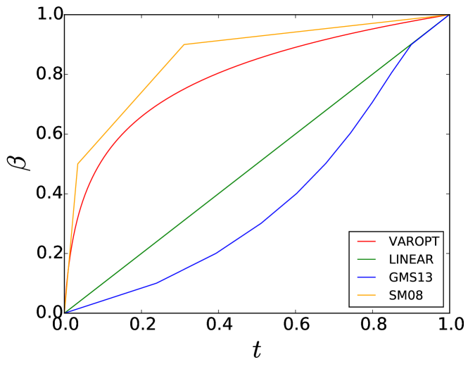
Figure 1: Comparison of annealing schedules for an RBM trained on MNIST by using PCD.

PCD(20)                                     CD1(20)                                    CD25(20)

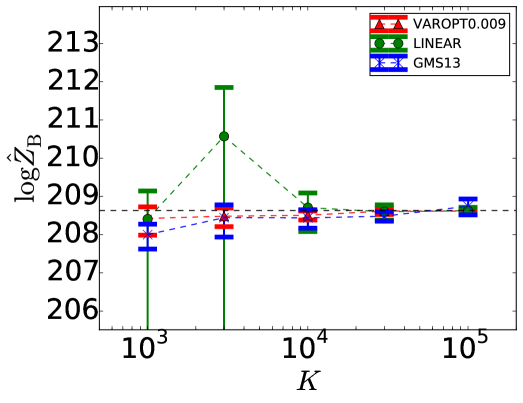
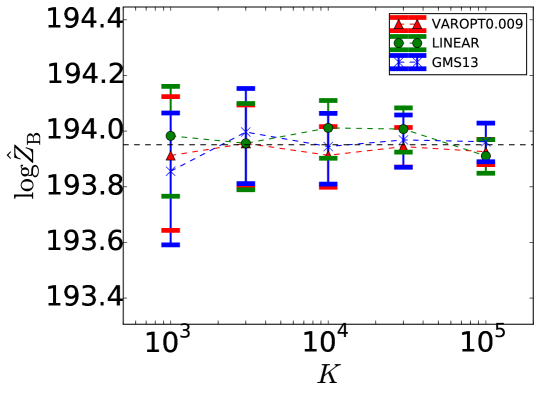
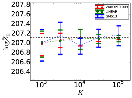
Figure 2: $\log\hat{Z}_{\mathrm{B}}$ for tractable RBMs as a function of $K$. Error bar shows $\pm 3\sigma$ intervals of $\log w$. The black broken lines indicate the ground truth.

PCD(20)                                     CD1(20)                                    CD25(20)

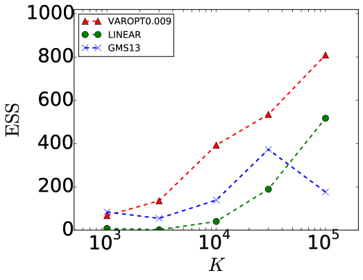
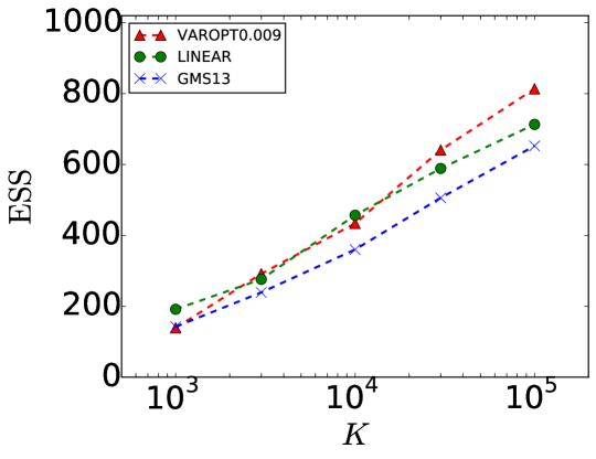
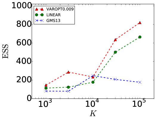
Figure 3: Estimates of the ESS’s plotted as a function of $K$.

Because the variance becomes inversely proportional to $K$ as $K$ increases, we analyze the behavior of $K\mathrm{Var}\left[\log w\right]$ for large $K$. By approximating the difference in the r.h.s. of Eq. (6) with a Taylor series up to fist order, we have the following approximation

$$K\mathrm{Var}\left[\log w\right] \approx K\sum_{k=0}^{K}(\Delta\beta_{k})^{2}{\mathrm{Var}_{\beta_{k}}}\left[\frac{\partial}{\partial\beta}\log p^{*}_{\beta}({\bf v})\right].$$ (7)

Assume that annealing schedule $\{\beta_{k}\}$ has a continuous limit i.e., $\beta_{k}=\beta(k/K)$ with some smooth function $\beta(t)$ defined on $t\in[0,1]$. Because the error caused by the approximation vanishes under this assumption as $K\rightarrow\infty$, the scaled variance asymptotically approaches a functional ${\cal J}(\beta(\cdot))$.

Theorem 1.

Assume perfect transitions. Assume that $\{\beta_{k}\}$ are composed as $\beta_{k}=\beta(t_{k})$ where $\beta(t)$ is a smooth function ($\beta(t)\in{\cal C}^{2}$) defined on $t\in[0,1]$ and $t_{k}=k/K$. Then as $K\rightarrow\infty$ the AIS estimation error behaves as:

$$K\mathrm{Var}\left[\log w\right]\rightarrow{\cal J}(\beta(\cdot))\triangleq\int_{0}^{1}\dot{\beta}^{2}g(\beta)\mathrm{d}t,$$ (8)

where $\dot{\beta}$ denotes the derivative of $\beta(t)$, i.e., $\frac{\mathrm{d}\beta(t)}{\mathrm{d}t}$, and $g(\beta)$ is a function defined as $g(\beta)\triangleq{\mathrm{Var}_{\beta}}\left[\frac{\partial}{\partial\beta}\log p^{*}_{\beta}({\bf v})\right]$. [See supplementary material for proof.]

Table 1: Estimates of the partition functions and the ESS’s for tractable RBMs. The ground truth of the estimate $\log Z_{\mathrm{B}}$ is also reported. All the figures are obtained with $K=100,000$

	PCD(20)			CD1(20)			CD25(20)
schedule	$\log Z_{\mathrm{B}}$	$\log\hat{Z}_{\mathrm{B}}$	ESS	$\log Z_{\mathrm{B}}$	$\log\hat{Z}_{\mathrm{B}}$	ESS	$\log Z_{\mathrm{B}}$	$\log\hat{Z}_{\mathrm{B}}$	ESS
VAROPT	208.63	208.629	783	193.951	194.117	87	207.12	207.136	776
VAROPT0.009		208.616	809		193.926	814		207.119	820
VAROPT0.006		208.643	668		193.937	803		207.148	751
VAROPT0.003		208.626	749		193.956	797		207.136	617
LINEAR		208.626	517		193.911	713		207.099	664
GMS13		208.745	176		193.962	653		207.175	176

$K=1,000$                           $10,000$                              $100,000$

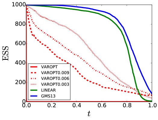
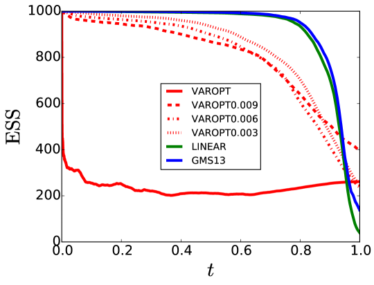
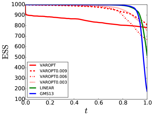
Figure 4: Evolution of the ESS’s on various $K$. These plots are computed with PCD(20)

Here the problem of finding the optimal schedule that minimizes the estimation error is formulated as a variational minimization problem of the functional ${\cal J}(\beta(\cdot))$ w.r.t. $\beta(\cdot)$. From Euler-Lagrange equation (Bishop, 2006), we derived the following differential equation that the optimal schedule obeys:

$$\ddot{\beta}+\frac{\dot{\beta}^{2}}{2}\frac{\mathrm{d}}{\mathrm{d}\beta}\log g(\beta)=0.$$ (9)

5 Numerical Search for The Optimal Schedule

By numerically solving Eq. (9) with boundary conditions $\beta(0)=0$ and $\beta(1)=1$, we can find the optimal schedule. A problem here is that $g(\beta)$ is intractable. To overcome this difficulty, we propose VAROPT-AIS algorithm listed in Algorithm 2 where we perform AIS twice; $g(\beta)$ is estimated by the first (cheap) execution of AIS with the linear scheduling, and $\log Z_{\mathrm{B}}$ is estimated by the second (expensive) execution of AIS with a schedule computed from the first execution. A key idea of VAROPT-AIS is to execute cheap AIS first to roughly survey the terrain through the annealing path i.e., $g(\beta)$, and then execute expensive AIS to gain thorough estimation.

In VAROPT-AIS, we use the method of fixed point iteration (Kelley, 1995) to solve the differential equation of Eq. (9) (labeled as DESolve in Algorithm 2). Because the l.h.s. of Eq. (9) does not directly depend on $g(\beta)$, we perform numerical differentiation to approximate $\frac{\mathrm{d}}{\mathrm{d}\beta}\log g(\beta)$ as preprocessing. We also perform convolutional smoothing of $g(\beta)$ estimates to remove less important noises.

Because Eq. (9) is derived based on the assumption of perfect transitions, the solution of Eq. (9) can have large ${\Delta\beta_{k}}=\beta_{k}-\beta_{k-1}$ that can impede the mixing of Markov chains. This can damage the estimation accuracy of AIS. To ease this effect, we optionally decelerate an annealing schedule s.t. $\max{\Delta\beta_{k}}\leq{\Delta\beta_{\mathrm{max}}}$ with Algorithm 3. This heuristic algorithm sequentially clips ${\Delta\beta_{k}}$ by ${\Delta\beta_{\mathrm{max}}}$ and stretches all ${\Delta\beta_{k}}$ to compensate the error caused by clipping.

6 Remarks

The methodology developed in this paper can be applied to various kinds of stochastic models to which AIS is applicable. Nevertheless, we are mainly interested in RBMs and only perform experiments on RBMs in this paper.

Also note that our method can be combined with various kinds of established techniques for AIS. First, the proposed method can be combined with HAIS (Sohl-Dickstein & Culpepper, 2012) because the selection of an annealing schedule is independent of the implementation of Markov transitions. Second, the proposed method can be used to schedule various types of annealing paths possibly including the moment averaging path with geometric interpolation (Grosse et al., 2013). Finally, the proposed method will easily be combined with a technique for tuning a proposal distribution (Kiwaki & Aihara, 2014).

Figure 1 compares an annealing schedule by our method (labeled as VAROPT) with those by several others: (LINEAR) the linear schedule that corresponds to $\beta(t)=t$; (GMS13) a scheme suggested by Grosse et al. (2013); and (SM08) a heuristic schedule suggested by Salakhutdinov & Murray (2008). Several interesting points can be seen from these plots. First, GMS13 is largely different from VAROPT and is rather similar to the linear schedule. This clearly shows that our objective ${\cal J}(\beta(\cdot))$ is intrinsically different from the objective proposed by Grosse et al. (2013). Second, VAROPT is similar to the heuristic schedule by Salakhutdinov & Murray (2008). This remarkable coincidence suggests that our proposal possibly automates expensive heuristic search of annealing schedules with human hands.

PCD(500)                                     CD1(500)                                    CD25(500)

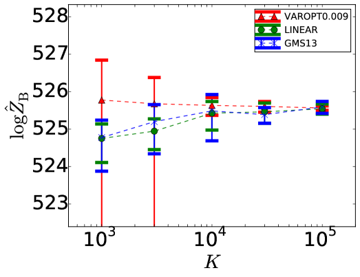
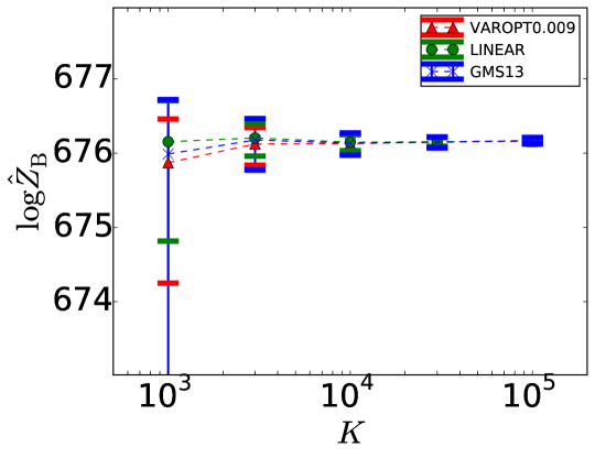
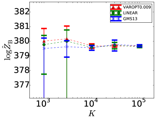
Figure 5: $\log\hat{Z}_{\mathrm{B}}$ for intractable RBMs as a function of $K$. Error bar shows $\pm 3\sigma$ intervals of $\log w$.

PCD(500)                                     CD1(500)                                    CD25(500)

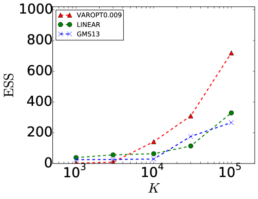
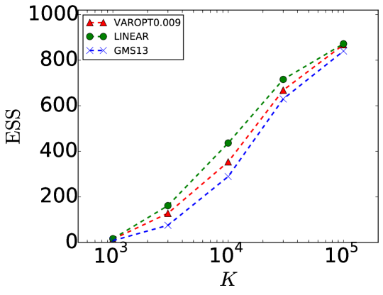
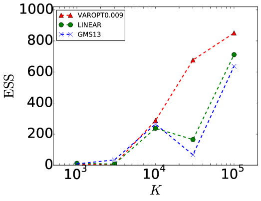
Figure 6: ESS estimates for intractable RBMs as a function of $K$.

7 Experiments

To demonstrate the benefits of the proposed method, we performed partition function estimation for several RBMs with various annealing schedules. We evaluated scheduling schemes with respect to two measures: ESS estimates and $\log\hat{Z}_{\mathrm{B}}$. As Neal (2001) warns, ESS estimates can be misleading if AIS fails to find important major modes of $p_{\mathrm{B}}$, and therefore one should be careful when reporting the estimates. In our experiments, however, we regard that ESS estimates are reliable because the partition function estimates seem reliable in most cases from comparison with the ground truth or from comparison with estimates by different schemes.

RBMs were trained on MNIST by using three training algorithms: (PCD) persistent contrastive divergence (Tieleman, 2008), (CD1) contrastive divergence (CD) with 1 step of state update, and (CD25) CD with 25 steps (Hinton, 2002). We label RBMs with the training algorithm and the number of hidden units; for example, PCD(500) denotes an RBM with 500 hidden units trained by PCD.

All the executions of AIS followed the geometric path. We fixed the number of AIS runs as $N=1,000$ and explored various magnitudes of $K\in 10^{[3,5]}$.

We mainly compared following three scheduling techniques: GMS13, LINEAR, and VAROPT. VAROPT schedules were computed with $\tilde{N}=100$ and $\tilde{K}=1,000$. Note that the computation required to gain VAROPT schedules was not heavy and negligible compared to the cost of the following main execution of AIS. In addition to simple VAROPT, we also tested decelerated VAROPT schedules with ${\Delta\beta_{\mathrm{max}}}\in\{0.003,0.006,0.009\}$. Decelerated schedules are labels as VAROPT${\Delta\beta_{\mathrm{max}}}$.

GMS13 schedules are determined using 10 different points of RBM parameters (knots) on the geometric path. On each knot, we estimated the moments of the RBM using 1,000 Markrov chains with 6,000 updates including 1,000 steps of burn-in updates.

7.1 Experiments with Small Tractable RBMs

We first show results with RBMs that have only 20 hidden units. Note that we can compute the exact value of $\log Z_{\mathrm{B}}$ for these RBMs by summing all the $2^{20}$ possible states of hidden units. For training RBMs, we used a fixed learning rate and performed 250,000 parameter updates.

The results of estimates are summarized in Table 1. It is remarkable to note that VAROPT0.009 achieves the highest ESS’s for all the RBMs. Estimates of $\log Z_{\mathrm{B}}$ and the ESS’s are plotted as a function of $K$ in Figs. 2 and 3. Note that the proposed method is solely represented by VAROPT0.009 in these plots. From these plots, it can be observed that VAROPT0.009 achieves the smallest estimation errors and the greatest ESS’s in most of the cases, especially with large $K$.

To better understand the behavior of VAROPT, we computed ESS estimates with on-the-fly AIS weights as shown in Fig. 4. Note that such on-the-fly ESS’s are valid statistics because on-the-fly AIS weights can be used to estimate the statistics of the intermediate distributions. Because the estimation error is accumulated throughout annealing (as Eq. (6) suggests), monitoring on-the-fly ESS estimates helps us to understand the characteristics of annealing schedules. It can be seen from Fig. 4 that VAROPT has a steep drop in the ESS’s at very the beginning of the annealing. Is is also shown that deceleration effectively relaxes this problem to yield higher ESS’s. We understand that this sudden drop in the ESS’s is due to poor mixing of Markov chains because the drop becomes smaller with larger value of $K$. Therefore, the larger $K$ becomes, the better estimation accuracy VAROPT enjoys.

Table 2: Estimates of the partition functions and the ESS’s for intractable RBMs. All the figures are obtained with $K=100,000$

	PCD(500)		CD1(500)		CD25(500)
schedule	$\log\hat{Z}_{\mathrm{B}}$	ESS	$\log\hat{Z}_{\mathrm{B}}$	ESS	$\log\hat{Z}_{\mathrm{B}}$	ESS
VAROPT	525.55	726	676.149	865	379.68	545
VAROPT0.009	525.564	719	676.158	868	379.687	851
VAROPT0.006	525.529	728	676.169	855	379.682	852
VAROPT0.003	525.548	661	676.13	873	379.68	778
LINEAR	525.545	329	676.167	872	379.628	712
GMS13	525.593	266	676.17	840	379.696	637

7.2 Experiments with Intractable RBMs

We next report estimation on intractable RBMs with 500 hidden units. RBMs were trained using randomly sampled hyperparameters such as the number of training epochs, learning rates, and L2 regularization.

Estimates of $\log Z_{\mathrm{B}}$ and the ESS’s are plotted in Figs. 5 and 6. Table 2 shows the $\log Z_{\mathrm{B}}$ and ESS estimates for $K=100,000$. The scores by (decelerated) VAROPT here look less appealing than for tractable RBMs. Especially, (decelerated) VAROPT exhibits large estimation errors for small $K$. This is possibly due to poorer mixing of RBMs with a larger number of hidden units. Nevertheless, estimation errors with (decelerated) VAROPT are rapidly reduced as $K$ increases. Thus, decelerated VAROPT schedules achieve greater ESS’s than the conventional scheduling schemes for all the RBMs with $K=100,000$ as in Table 2.

8 Conclusion

We pursued a problem of determining the optimal annealing schedule for AIS. Assuming perfect transition, we derived a functional that dominates the estimation error and formulated the problem as a variational minimization problem. We developed a numerical scheme to solve this variational problem and implemented a practical algorithm to approximate the optimal annealing schedule. We performed experiments and demonstrated that the proposed algorithm achieved better estimation accuracy than conventional schemes in most cases with a large number of intermediate distributions.

Appendix A Derivation of Eq. (7)

By Taylor series expansion of $\log p^{*}_{\beta}({\bf v})$ w.r.t. $\beta$, the variance $\mathrm{Var}\left[\log w\right]$ can be written as

$$\mathrm{Var}\left[\log w\right]=\sum_{k=0}^{K}{\mathrm{Var}_{\beta_{k}}}\left[\log p^{*}_{\beta_{k+1}}({\bf v})-\log p^{*}_{\beta_{k}}({\bf v})\right]$$ (10)

$$=\sum_{k=0}^{K}{\mathrm{Var}_{\beta_{k}}}\left[\frac{\partial}{\partial\beta}\log p^{*}_{\beta}({\bf v}){\Delta\beta_{k}}+\delta({\bf v},\beta_{k})O({\Delta\beta_{k}}^{2})\right],$$ (11)

where we defined ${\Delta\beta_{k}}=\beta_{k+1}-\beta_{k}$, and the coefficients for the higher order terms are represented by $\delta({\bf v},\beta_{k})$. Because ${\Delta\beta_{k}}$ does not depend on ${\bf v}$, $K\mathrm{Var}\left[\log w\right]$ can be further rewritten as

$$\mathrm{Var}\left[\log w\right]$$

$$=\sum_{k=0}^{K}\left\{{\Delta\beta_{k}}^{2}{\mathrm{Var}_{\beta_{k}}}\left[\frac{\partial}{\partial\beta}\log p^{*}_{\beta}({\bf v})\right]+\delta(\beta_{k})O({\Delta\beta_{k}}^{3})\right\}$$ (12)

where $\delta(\beta_{k})=2\mathrm{Cov}_{\beta_{k}}\left[\delta({\bf v},\beta_{k}),\frac{\partial}{\partial\beta}\log p^{*}_{\beta}({\bf v})\right]$ with $\mathrm{Cov}_{\beta_{k}}$ being the covariance operator w.r.t. $p_{\beta}$. Neglect of the second term of the r.h.s. yields Eq. (7).

Appendix B Proof of Theorem 1

Theorem 1.

Assume perfect transitions. Assume that $\{\beta_{k}\}$ are composed as $\beta_{k}=\beta(t_{k})$ where $\beta(t)$ is a smooth function ($\beta(t)\in{\cal C}^{2}$) defined on $t\in[0,1]$ and $t_{k}=k/K$. Then as $K\rightarrow\infty$ the AIS estimation error behaves as:

$$K\mathrm{Var}\left[\log w\right]\rightarrow{\cal J}(\beta(\cdot))\triangleq\int_{0}^{1}\dot{\beta}^{2}g(\beta)\mathrm{d}t,$$ (13)

where $\dot{\beta}$ denotes the derivative of $\beta(t)$, i.e., $\frac{\mathrm{d}\beta(t)}{\mathrm{d}t}$, and $g(\beta)$ is a function defined as $g(\beta)\triangleq{\mathrm{Var}_{\beta}}\left[\frac{\partial}{\partial\beta}\log p^{*}_{\beta}({\bf v})\right]$.

Proof.

From Eq. (B), the scaled variance is written as

$$K\mathrm{Var}\left[\log w\right]= \frac{1}{K}\sum_{k=0}^{K}\left(K{\Delta\beta_{k}}\right)^{2}{\mathrm{Var}_{\beta_{k}}}\left[\frac{\partial}{\partial\beta}\log p^{*}_{\beta}({\bf v})\right]$$

$$+K\sum_{k=0}^{K}\delta(\beta_{k})O({\Delta\beta_{k}}^{3}),$$

The second term of the r.h.s. vanishes if $K\rightarrow\infty$ as $\left|K\sum_{k=0}^{K}\delta(\beta_{k})O({\Delta\beta_{k}}^{3})\right|\leq CK\sum_{k=0}^{K}\delta(\beta_{k})\left|{\Delta\beta_{k}}^{3}\right|<C\tilde{C}^{3}K\sum_{k=0}\delta(\beta_{k})\left|t_{k+1}-t_{k}\right|^{3}=O(K^{-1})\rightarrow 0$ with $\exists\tilde{C},C>0$. Note that we have $\left|\beta_{k+1}-\beta_{k}\right|<\tilde{C}\left|t_{k+1}-t_{k}\right|$ because $\beta(t)(\in{\cal C}^{2})\in{\cal C}^{1}$ and $|\delta(\beta)|<\infty$ because $p_{\beta}$ is smooth. The scaled variance is dominated by the first term of the r.h.s., which have the following limit as $K\rightarrow\infty$

$${\cal J}(\beta(\cdot))\triangleq\int_{0}^{1}\dot{\beta}^{2}{\mathrm{Var}_{\beta}}\left[\frac{\partial}{\partial\beta}\log p^{*}_{\beta}({\bf v})\right]\mathrm{d}t.$$ (14)

Therefore, $K\mathrm{Var}\left[\log w\right]\rightarrow{\cal J}(\beta(\cdot))$. ∎

Appendix C Derivation of Eq. (9)

Euler-Lagrange equation for ${\cal J}(\beta(\cdot))$ is

$$\frac{\mathrm{d}}{\mathrm{d}t}\left(\frac{\partial G}{\partial\dot{\beta}}\right)=\frac{\partial G}{\partial\beta},$$ (15)

where $G\triangleq\dot{\beta}^{2}g(\beta)$. The l.h.s. is computed as $\frac{\mathrm{d}}{\mathrm{d}t}(2\dot{\beta}g(\beta))=2(\ddot{\beta}g(\beta)+\frac{\mathrm{d}g}{\mathrm{d}\beta}\dot{\beta}^{2})$. The r.h.s. is computed as $\frac{\mathrm{d}g}{\mathrm{d}\beta}\dot{\beta}^{2}$. By replacing both sides of Eq. (15) with these results, we have $\ddot{\beta}+\frac{1}{2g}\frac{\mathrm{d}g}{\mathrm{d}\beta}\dot{\beta}^{2}=\ddot{\beta}+\frac{\dot{\beta}^{2}}{2}\frac{\mathrm{d}}{\mathrm{d}\beta}\log g(\beta)=0$

References

- Behrens et al. (2012) Behrens, Gundula, Friel, Nial, and Hurn, Merrilee. Tuning Tempered Transitions. Statistics and Computing, 22:65–78, December 2012.
- Bishop (2006) Bishop, Christopher M. Pattern Recognition and Machine Learning. Springer Verlag, August 2006.
- Dauphin & Bengio (2013) Dauphin, Y and Bengio, Y. Stochastic Ratio Matching of RBMs for Sparse High-Dimensional Inputs. In Advances in Neural Information Processing Systems 26, 2013.
- Desjardins et al. (2013) Desjardins, Guillaume, Pascanu, Razvan, Courville, Aaron, and Bengio, Yoshua. Metric-Free Natural Gradient for Joint-Training of Boltzmann Machines. arXiv.org, January 2013.
- Gelman & Meng (1998) Gelman, A and Meng, X L. Simulating normalizing constants: From importance sampling to bridge sampling to path sampling. Statistical science, 13(2):163–185, May 1998.
- Grosse et al. (2013) Grosse, Roger B, Maddison, Chris J, and Salakhutdinov, Ruslan. Annealing between distributions by averaging moments. pp. 2769–2777, 2013.
- Hinton (2002) Hinton, Geoffrey E. Training products of experts by minimizing contrastive divergence. Neural Computation, 14(8):1771–1800, August 2002.
- Iba (2001) Iba, Yukito. Extended Ensemble Monte Carlo. International Journal of Modern Physics, pp. 623–656, 2001.
- Kelley (1995) Kelley, C T. Iterative Methods for Linear and Nonlinear Equations. SIAM, 1995.
- Kiwaki & Aihara (2014) Kiwaki, Taichi and Aihara, Kazuyuki. On Importance of Base Model Covariance for Annealing Gaussian RBMs . In Deep Learning and Representation Learning Workshop: NIPS 2014, 2014.
- Neal (1996) Neal, Radford M. Sampling from multimodal distributions using tempered transitions. Statistics and Computing, 6(4):353–366, 1996.
- Neal (2001) Neal, Radford M. Annealed Importance Sampling. Statistics and Computing, 11:125–139, 2001.
- Ogata (1989) Ogata, Yosihiko. A Monte Carlo method for high dimensional integration. Numerische Mathematik, 55(2):137–157, 1989.
- Salakhutdinov & Hinton (2009) Salakhutdinov, Ruslan and Hinton, Geoffrey E. Replicated softmax: an undirected topic model. In Advances in Neural Information Processing Systems 22, pp. 1607–1614, 2009.
- Salakhutdinov & Murray (2008) Salakhutdinov, Ruslan and Murray, Iain. On the quantitative analysis of deep belief networks. In Proceedings of the 25th International Conference on Machine Learning. ACM, July 2008.
- Sohl-Dickstein & Culpepper (2012) Sohl-Dickstein, Jascha and Culpepper, Benjamin J. Hamiltonian Annealed Importance Sampling for partition function estimation. Technical report, May 2012.
- Tieleman (2008) Tieleman, Tijmen. Training restricted Boltzmann machines using approximations to the likelihood gradient. In Proceedings of the 25th International Conference on Machine Learning, pp. 1064–1071. ACM, July 2008.
- Yedidia et al. (2005) Yedidia, Jonathan S, Freeman, William T, and Weiss, Yair. Constructing free-energy approximations and generalized belief propagation algorithms. Information Theory, IEEE Transactions on, 51(7):2282–2312, 2005.