Finite-size effects in the spectrum of the $OSp(3|2)$ superspin chain

Abstract

The low energy spectrum of a spin chain with $OSp(3|2)$ supergroup symmetry is studied based on the Bethe ansatz solution of the related vertex model. This model is a lattice realization of intersecting loops in two dimensions with loop fugacity $z=1$ which provides a framework to study the critical properties of the unusual low temperature Goldstone phase of the $O(N)$ sigma model for $N=1$ in the context of an integrable model. Our finite-size analysis provides strong evidence for the existence of continua of scaling dimensions, the lowest of them starting at the ground state. Based on our data we conjecture that the so-called watermelon correlation functions decay logarithmically with exponents related to the quadratic Casimir operator of $OSp(3|2)$. The presence of a continuous spectrum is not affected by a change to the boundary conditions although the density of states in the continua appears to be modified.

I Introduction

This paper is concerned with the study of the finite-size properties of a solvable two-dimensional vertex model based on the five-dimensional representation of the $OSp(3|2)$ superalgebra. This system has a close relation with a particular Lorentz lattice gas used to model the diffusion of particles through randomly placed obstacles on the square lattice Martins et al. (1998). In this cellular automata the particle moves along the bonds of the lattice and is scattered according to scattering rules fixed a priori once it reaches a given node. Here the scatterers are constituted of mirrors tilted right and left, i.e. by $\pm\frac{\pi}{4}$, with respect to the lattice Ruijgrok and Cohen (1988); Gunn and Ortuño (1985). When the particle collides with a mirror it will turn right or left, depending on the orientation of the latter. In the absence of a mirror at a node the particle passes the node on a straight path. The corresponding scattering rules are depicted in Figure 1.

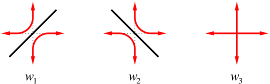
Figure 1: Scattering rules for right mirrors, left mirrors and empty sites. The different vertices appear with probabilities $w_{1}$, $w_{2}$, $w_{3}$ respectively.

Amplitudes $w_{1}$, $w_{2}$ and $w_{3}$ represent the fraction of right and left mirrors and node vacancies on the lattice, respectively. The kinetic properties of this lattice Lorentz gas have been investigated by numerical simulations where an anomalous diffusive behavior was observed Ziff et al. (1991). In the case of partially occupied lattice by mirrors ($w_{3}\neq 0$) the fractal dimension of large trajectories was argued to be $d_{f}=2$ with the presence of logarithmic corrections Owczarek and Prellberg (1995); Cao and Cohen (1997).

An alternative interpretation of the paths of particles in this lattice gas is in terms of the degrees of freedom of an intersecting loop model with periodic boundary conditions in both lattice directions imposed. In Figure 2 we show the three possible configurations of a node of such loop model together with their corresponding probabilities.

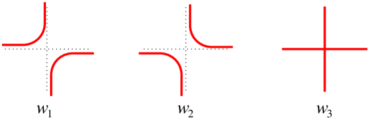
Figure 2: The possible configurations of a node in the intersecting loop model and their associated Boltzmann weights $w_{1}$, $w_{2}$, $w_{3}$.

Weighting every closed loop in a given state by a fugacity $z$ the object of our study is the partition function,

$$Z=\sum_{\mathrm{loop~{}configurations}}w_{1}^{m_{1}}\,w_{2}^{m_{2}}\,w_{3}^{m_{3}}\,z^{\cal{N}}\,,$$ (1)

where $m_{1}$, $m_{2}$ and $m_{3}$ are the number of weights $w_{1}$, $w_{2}$ and $w_{3}$ and $\cal{N}$ denotes the number of loops on a such statistical configuration.

For the case of fugacity $z=1$ this intersecting loop model can be reformulated as the $OSp(3|2)$ supersymmetric vertex model which is the subject of this paper. The integrability of this model provides a framework for the study of its critical behaviour and – exploiting the equivalences listed above – of the peculiar properties observed in the Lorentz lattice gas. In fact, the finite-size analysis of the lowest excitation of the $OSp(3|2)$ superspin chain found the respective critical exponent to be very small Martins et al. (1998). This was taken as an indication for the presence of a zero conformal dimension on the spectrum implying the superdiffusive behaviour ($d_{f}=2$) predicted for the Lorentz gas.

In the context of the loop model, it has been argued that this behaviour signals the existence of an unusual critical phase of intersecting loops: in two dimensions the crossing of loops, $w_{3}\neq 0$, is a relevant perturbation to the low temperature dense loops phase Jacobsen et al. (2003). As a consequence the long distance behaviour of correlation functions in the loop model with fugacity of closed loops $z=N<2$ should be that of the Goldstone phase of the $O(N)$ sigma model. For integer $N$ this regime can be described in a supersymmetric formulation of the field theory in terms of $m$ bosons and $2n$ symplectic fermions, $N=m-2n$. The $OSp(3|2)$ vertex model is one from a class of integrable lattice regularizations of these models. Their central charges are $c=N-1$ as expected in the Goldstone phase Martins et al. (1998).

There has been a series of attempts towards the identification of the other characteristic feature of this Goldstone phase starting from integrable lattice models, i.e. a finite density of vanishing critical exponents. The existence of a continuous spectrum of conformal weights has been established in several staggered superspin chains Essler et al. (2005); Frahm and Martins (2011); Vernier et al. (2014), including a model based on the four-dimensional representations of $U_{q}[sl(2|1)]$ alternating with their duals which, in the self-dual case, is isomorphic a deformation of the $OSp(2|2)$ chain relevant to the loop model with fugacity $N=0$ Frahm and Martins (2012). Further details of the spectral properties of these models have been uncovered when it was realized that hidden within the zero charge sector of this superspin chain there exists a staggered six-vertex model which already displays a continuous low energy spectrum. For the latter strong evidence has been accumulated that the effective theory describing the low energy excitations of the model is the $SL(2,\mathbb{R})/U(1)$ sigma model at a level related to the anisotropy Ikhlef et al. (2008, 2012); Candu and Ikhlef (2013); Frahm and Seel (2014). We note, however, that the focus of these studies has been on the anisotropic deformations of the vertex models: while it has been established that the isotropic $N=0$ models are on the boundary of the critical region, the question of the critical properties at the isotropic point itself has not been addressed.

In this paper we want to return to the case of $N=1$ as described by the $OSp(3|2)$ supersymmetric vertex model. As argued above, the critical properties of this model are those of the proposed Goldstone phase of the $O(1)$ sigma model and can be studied based on its solutions by means of the algebraic Bethe ansatz. By means of an extensive finite-size study of the model we accumulate ample evidence for the existence of continua of critical exponents with lower edges at scaling dimensions $X=0$, $1$, $2$, $4$, $6$,… . With the exception of the the ground state of the superspin chain all of the states considered show strong logarithmic corrections to scaling governed by the flow of the model to weak coupling in the Goldstone phase. This is complemented by the observation that many excitations which have energies $\propto 1/L$ for small system sizes but disappear from the low energy spectrum as the system size is increased. Both of these features of the spectrum require very large system sizes to be studied for a reliable identification of the low energy effective theory: here we consider lattices with up to $4096$ sites.

Finally, since recent numerical studies of the $N=1$ intersecting loop model have emphasized the importance of boundary conditions for the long distance behaviour of correlation functions Kager and Nienhuis (2006); Nahum et al. (2013) we consider both periodic boundary conditions to the superspin chain and twisted ones depending on the fermion number. Comparing the results we find that the amplitudes of the subleading (logarithmic in the system size) finite-size corrections do depend on the choice of boundary conditions.

II The integrable lattice model

The statistical configurations of the Lorentz lattice gas or intersecting loop model mentioned in the introduction have a one-to-one correspondence with the generators of the braid-monoid algebra. This fact has been elaborated previously in the work Martins et al. (1998) but for sake of completeness we have summarized this equivalence in Appendix A. This algebra can be used to built solvable models and it turns out that integrability is assured when the weights are parameterized as

$$w_{1}=w_{0},\quad w_{2}=\frac{w_{0}\lambda}{1/2-\lambda},\quad w_{3}=w_{0}\lambda$$ (2)

where $\lambda$ is a free spectral parameter and $w_{0}$ is an arbitrary normalization. This scale can be chosen to interpret the weights as probabilities but in our context we set it to unity. Note that all three weights are positive for $0\leq\lambda\leq\frac{1}{2}$.

Furthermore, it has been shown that this integrable manifold can be realized in terms of a standard local vertex model. Its bond states are constituted of three bosonic and two fermionic degrees of freedom realized in terms of the five-dimensional representation of the $OSp(3|2)$ superalgebra, see Appendix B. The possible configurations on a vertex with their respective Boltzmann weights are encoded in the $R$-matrix

$${R}_{0j}(\lambda)=\sum_{a,b=1}^{5}\left[w_{1}(-1)^{p_{a}p_{b}}e_{ab}^{(0)}\otimes e_{ba}^{(j)}+w_{2}\sum_{c,d=1}^{5}\alpha_{ab}\alpha_{cd}^{-1}e_{ac}^{(0)}\otimes e_{bd}^{(j)}+w_{3}e_{ab}^{(0)}\otimes e_{ab}^{(j)}\right]$$ (3)

where $e_{ab}^{(k)}$ are the $5\times 5$ Weyl matrices acting either on the auxiliary space for $k=0$ or on the quantum space associated to the sites of a chain of length ${L}$ for $k=1,\cdots,{L}$. The symbol $p_{a}$ denotes the Grassmann parities distinguishing the bosonic ($p_{a}=0$) and fermionic ($p_{a}=1$) degrees of freedom. The $5\times 5$-matrix $\alpha_{ab}$ is the basic ingredient to built an explicit representation for the monoid operator and its expression depends much on the grading order basis, see for instance Martins and Ramos (1997). Here we will consider two specific Grassmann orderings in which the two ${U}(1)$ charges of the $OSp(3|2)$ algebra commuting with the operator ${R}_{0j}(\lambda)$ are organized in a way which is suitable to perform the Bethe ansatz analysis. This turns out to be the ${fbbbf}$ and ${bfbfb}$ basis ordering and the corresponding forms for the matrix $\alpha$ are

$$\alpha^{(fbbbf)}=\left(\begin{array}[]{ccccc}0&0&0&0&1\\ 0&0&0&1&0\\ 0&0&1&0&0\\ 0&1&0&0&0\\ -1&0&0&0&0\\ \end{array}\right),\quad\alpha^{(bfbfb)}=\left(\begin{array}[]{ccccc}0&0&0&0&1\\ 0&0&0&-1&0\\ 0&0&1&0&0\\ 0&1&0&0&0\\ 1&0&0&0&0\\ \end{array}\right).$$ (4)

For the vertex model on the square lattice with $L\times L$ vertices and periodic boundary conditions for both bosonic and fermionic configurations in the horizontal direction we now construct the vertex model row-to-row transfer matrix. This operator is given as the supertrace over the auxiliary space of an ordered product of ${L}$ matrices ${R}_{0j}(\lambda)$,

$${T}(\lambda)=\sum_{a=1}^{5}(-1)^{p_{a}}\left[{R}_{0{L}}(\lambda){R}_{0{L}-1}(\lambda)\cdots{R}_{01}(\lambda)\right]_{aa}\,.$$ (5)

As a consequence of integrability the transfer matrix commutes for different values of the spectral parameter, $[T(\lambda),T(\mu)]=0$, and therefore generates a family of commuting operators. As usual, a Hamiltonian with local (nearest neighbour on the lattice) interactions is obtained by expanding (5) around the point $\lambda=0$ where the transfer matrix becomes proportional to the translation operator. The resulting expression for the integrable $OSp(3|2)$ superspin Hamiltonian is

$${H}=-\sum_{j=1}^{L}\left[\sum_{a,b=1}^{5}(-1)^{p_{a}p_{b}}e_{ab}^{(j)}\otimes e_{ba}^{(j+1)}+2\sum_{a,b,c,d=1}^{5}\alpha_{ab}\alpha_{cd}^{-1}e_{ac}^{(j)}\otimes e_{bd}^{(j+1)}\right]\,,$$ (6)

where periodic boundary conditions for bosonic and fermionic degrees of freedom are assumed.

In terms of the transfer matrix the partition function of the vertex model is given by a supertrace of the $L^{\mathrm{th}}$ power of $T(\lambda)$, now taken on the $5^{L}$-dimensional quantum space. For system sizes up to $4\times 4$ we find by direct computation

$${Z}=\sum_{k=1}^{5^{L}}(-1)^{p_{1}^{k}+p_{2}^{k}\cdots+p_{{L}}^{k}}{T}_{kk}(\lambda)=\left[1+\lambda+\frac{\lambda}{1/2-\lambda}\right]^{{L}^{2}}\,$$ (7)

in agreement with the triviality of the partition sum (1) of the loop model with $z=1$. Here $p_{1}^{k},\cdots,p_{{L}}^{k}$ are the Grassmann parities of the degrees of freedom composing a given $k$-state of the Hilbert space. The partition function of any statistical model is dominated by the largest eigenvalue of the transfer matrix. In the present case the contribution of a single vertex to the partition function is the sum of the three weights $w_{1}+w_{2}+w_{3}$. Therefore, as long as the Boltzmann weights are all non-negative (i.e. in the regime $0\leq\lambda\leq 1/2$), we conclude that the largest eigenvalue of the transfer matrix $\Lambda_{{max}}(\lambda)$ for the lattice with linear dimension $L$ is

$$\Lambda_{{max}}(\lambda)=\left[1+\lambda+\frac{\lambda}{1/2-\lambda}\right]^{{L}}\,.$$ (8)

The fact that there are no subleading (in $L$) corrections is a consequence of the grading of the states together with the properties of the $OSp(3|2)$ representations appearing in the Hilbert space, see Appendix B.

We note that as an immediate consequence of the expression (8) for the largest eigenvalue of the transfer matrix the ground state energy of the superspin chain (6) is

$$E_{0}=-3L\,$$ (9)

without finite-size corrections.

Eq. (7) implies that the partition function can be normalized to $Z=1$ by rescaling of the local Boltzmann weights. Note that this does not necessarily mean that the low-lying excitations in the spectrum of the transfer matrix are trivial. In general, we can only infer that the critical properties are governed by a conformal field theory (CFT) with central charge $c=0$. Since the Hamiltonian (6) is a non-Hermitian operator the continuum limit is not expected to be described by a unitary $c=0$ conformal field theory.

In order to study the finite-size properties of the low-lying spectrum of this quantum spin chain we turn to its Bethe ansatz solution.

III The Bethe ansatz

The diagonalization of the transfer matrix can be carried out within the algebraic Bethe ansatz framework. The essential tools have already been discussed before Martins and Ramos (1997) and here we shall present only the main results. It turns out to be convenient to re-scale the spectral parameter by the imaginary unit to bring the resulting equations into a canonical form for performing numerical analysis. Denoting by $\Lambda(\lambda)$ the eigenvalues of the transfer matrix (5) we find that they can be parametrized in terms of two sets of rapidities $\{\lambda_{j}^{(a)}\}$, $a=1,2$. The functional form of the eigenvalues as well as the algebraic Bethe equations satisfied by the rapidities depend on the grading chosen.

III.1 Bethe ansatz in $fbbbf$ grading

The Hilbert space of the superspin chain can be decomposed into the irreducible representations (irreps) $(p;q)$ of $OSp(3|2)$ appearing in the tensor product $(0;\frac{1}{2})^{\otimes L}$ of local spins, see Appendix B. In the grading $fbbbf$ a highest weight state of the $(8L-4)$-dimensional representation $(L-1;\frac{1}{2})$ is used as pseudo vacuum (or reference state) for the algebraic Bethe ansatz. Thanks to the algebra inclusion ${OSp(3|2)}\supset{SU}(2)\oplus{SU}(2)$ all states can be characterized in terms of the two $U(1)$ charges $\ell^{z}$, $s^{z}$ from the $SU(2)$ subalgebras. In the reference state they take values $L$ and $0$, respectively. Bethe states in a $(p;q)$ multiplet are parametrized by $(L-n_{1})$ complex rapidities $\lambda_{j}^{(1)}$ and $(L-n_{1}-n_{2})$ complex rapidities $\lambda_{j}^{(2)}$, where

$$n_{1}=p+1\,,\quad n_{2}=2q-1\,$$ (10)

for all states except the $OSp(3|2)$ singlet $(0;0)$ for which $n_{1}=n_{2}=0$ (note that only $OSp(3|2)$ irreps with integer $p$ appear in the Hilbert space of the superspin chain).

The corresponding transfer matrix eigenvalue is given by the following expression:

$$\Lambda(\lambda)=-\left[\lambda/i-1\right]^{{L}}\prod_{j=1}^{{L-n_{1}}}\frac{\lambda-\lambda_{j}^{(1)}+i/2}{\lambda-\lambda_{j}^{(1)}-i/2}+\left[\lambda/i\right]^{{L}}\prod_{j=1}^{{L-n_{1}}}\frac{\lambda-\lambda_{j}^{(1)}+i/2}{\lambda-\lambda_{j}^{(1)}-i/2}\prod_{j=1}^{{L-n_{1}-n_{2}}}\frac{\lambda-\lambda_{j}^{(2)}-i}{\lambda-\lambda_{j}^{(2)}}$$ (11)

$$+\left[\lambda/i\right]^{{L}}\left\{\prod_{j=1}^{{L-n_{1}-n_{2}}}\frac{(\lambda-\lambda_{j}^{(2)}-i)}{(\lambda-\lambda_{j}^{(2)})}\frac{(\lambda-\lambda_{j}^{(2)}+i/2)}{(\lambda-\lambda_{j}^{(2)}-i/2)}+\prod_{j=1}^{{L-n_{1}}}\frac{\lambda-\lambda_{j}^{(1)}-i}{\lambda-\lambda_{j}^{(1)}}\prod_{j=1}^{{L-n_{1}-n_{2}}}\frac{\lambda-\lambda_{j}^{(2)}+i/2}{\lambda-\lambda_{j}^{(2)}-i/2}\right\}$$

$$-\left[\lambda\frac{(1/2-i\lambda)}{(-i/2+\lambda)}\right]^{{L}}\prod_{j=1}^{{L-n_{1}}}\frac{\lambda-\lambda_{j}^{(1)}-i}{\lambda-\lambda_{j}^{(1)}}\,.$$

The eigenspectrum of the Hamiltonian can be derived from this expression giving

$$E(\{\lambda_{j}^{(1)}\},\{\lambda_{j}^{(2)}\})=L-\sum_{j=1}^{{L-n_{1}}}\frac{1}{[\lambda_{j}^{(1)}]^{2}+1/4}\,.$$ (12)

The sets of variables $\{\lambda_{j}^{(a)}\}$ are constrained by the Bethe ansatz equations which for the ${fbbbf}$ grading are given by

$$\left[\frac{\lambda_{j}^{(1)}+i/2}{\lambda_{j}^{(1)}-i/2}\right]^{{L}} =\prod_{k=1}^{{L-n_{1}-n_{2}}}\frac{\lambda_{j}^{(1)}-\lambda_{k}^{(2)}+i/2}{\lambda_{j}^{(1)}-\lambda_{k}^{(2)}-i/2},\quad j=1,\cdots,{L-n_{1}},$$ (13)

$$\prod_{k=1}^{{L-n_{1}}}\frac{\lambda_{j}^{(2)}-\lambda_{k}^{(1)}+i/2}{\lambda_{j}^{(2)}-\lambda_{k}^{(1)}-i/2} =\prod_{k\neq j}^{{L-n_{1}-n_{2}}}\frac{\lambda_{j}^{(2)}-\lambda_{k}^{(2)}+i/2}{\lambda_{j}^{(2)}-\lambda_{k}^{(2)}-i/2},\quad j=1,\cdots,{L-n_{1}-n_{2}}\,.$$

III.2 Bethe ansatz in $bfbfb$ grading

In this grading the Bethe ansatz uses a highest weight state of the $(8L-4)$-dimensional representation $(0;L/2)$ as reference state. States in the sector $(p;q)$ with (10) are now parameterized by $(L-n_{2}-1)$ rapidities $\lambda_{j}^{(1)}$ and $(L-n_{1}-n_{2})$ rapidities $\lambda_{j}^{(2)}$). In terms of these parameters the corresponding transfer matrix eigenvalue is

$$\Lambda(\lambda)=\left[\lambda/i+1\right]^{{L}}\prod_{j=1}^{{L-n_{2}-1}}\frac{\lambda-\lambda_{j}^{(1)}-i/2}{\lambda-\lambda_{j}^{(1)}+i/2}-\left[\lambda/i\right]^{{L}}\prod_{j=1}^{{L-n_{2}-1}}\frac{\lambda-\lambda_{j}^{(1)}+i/2}{\lambda-\lambda_{j}^{(1)}+i/2}\prod_{j=1}^{{L-n_{1}-n_{2}}}\frac{\lambda-\lambda_{j}^{(2)}+i}{\lambda-\lambda_{j}^{(2)}}$$ (14)

$$+\left[\lambda/i\right]^{{L}}\left\{\prod_{j=1}^{{L-n_{1}-n_{2}}}\frac{(\lambda-\lambda_{j}^{(2)}-i)}{(\lambda-\lambda_{j}^{(2)})}\frac{(\lambda-\lambda_{j}^{(2)}+i/2)}{(\lambda-\lambda_{j}^{(2)}-i/2)}-\prod_{j=1}^{{L-n_{2}-1}}\frac{\lambda-\lambda_{j}^{(1)}}{\lambda-\lambda_{j}^{(1)}-i}\prod_{j=1}^{{L-n_{1}-n_{2}}}\frac{\lambda-\lambda_{j}^{(2)}-3i/2}{\lambda-\lambda_{j}^{(2)}-i/2}\right\}$$

$$\left[\lambda\frac{(3/2+i\lambda)}{(i/2-\lambda)}\right]^{{L}}\prod_{j=1}^{{L-n_{2}-1}}\frac{\lambda-\lambda_{j}^{(1)}}{\lambda-\lambda_{j}^{(1)}-i}\,.$$

The expression for energies of the Hamiltonian in this grading differs from the previous one by an overall minus sign:

$$E(\{\lambda_{j}^{(1)}\},\{\lambda_{j}^{(2)}\})=-L+\sum_{j=1}^{{L-n_{2}-1}}\frac{1}{[\lambda_{j}^{(1)}]^{2}+1/4}$$ (15)

The Bethe equations for the rapidities $\lambda_{j}^{(a)}$, $a=1,2$ in the grading $bfbfb$ are

$$\left[\frac{\lambda_{j}^{(1)}+i/2}{\lambda_{j}^{(1)}-i/2}\right]^{{L}} =\prod_{k=1}^{{L-n_{1}-n_{2}}}\frac{\lambda_{j}^{(1)}-\lambda_{k}^{(2)}+i/2}{\lambda_{j}^{(1)}-\lambda_{k}^{(2)}-i/2},\quad j=1,\cdots,{L-n_{2}-1},$$ (16)

$$\prod_{k=1}^{{L-n_{2}-1}}\frac{\lambda_{j}^{(2)}-\lambda_{k}^{(1)}+i/2}{\lambda_{j}^{(2)}-\lambda_{k}^{(1)}-i/2} =\prod_{k\neq j}^{{L-n_{1}-n_{2}}}\frac{(\lambda_{j}^{(2)}-\lambda_{k}^{(2)}-i/2)}{(\lambda_{j}^{(2)}-\lambda_{k}^{(2)}+i/2)}\frac{(\lambda_{j}^{(2)}-\lambda_{k}^{(2)}+i)}{(\lambda_{j}^{(2)}-\lambda_{k}^{(2)}-i)},\quad j=1,\cdots,{L-n_{1}-n_{2}}$$

Note that in this solution the inclusion ${OSp(3|2)}\supset{OSp(1|2)}$ becomes manifest: the second Bethe equations are exactly those of the ${OSp(1|2)}$ invariant vertex model in the presence of inhomogeneities Martins and Ramos (1997).

III.3 Example: $L=2$

For $L=2$ the spectrum of the superspin chain decomposes into the $OSp(3|2)$ singlet $(0;0)$ and two twelve-dimensional multiplets $(0;1)$ and $(1;\frac{1}{2})$, see Eq. (45). For these we can identify the corresponding Bethe root configurations in both gradings:

For the $fbbbf$ grading the Bethe equations are (13), the corresponding energy is (12). The three energies are

• $(1;\frac{1}{2})$ (the $fbbbf$ reference state):
  $L-n_{1}=0$ Bethe roots $\lambda^{(1)}$, $L-n_{1}-n_{2}=0$ Bethe roots $\lambda^{(2)}$: the energy of this state is $E=+2$.

• $(0;1)$:
  here we have $n_{1}=1$, $n_{2}=1$ according to (10). The only one finite solution to the Bethe equations (13) is $\lambda^{(1)}=0$ giving energy $E=-2$.

• $(0;0)$:
  for the singlet ground state the quantum numbers are $(n_{1},n_{2})=(0,0)$, therefore there are two roots $\lambda_{j}^{(a)}$ on each level, $a=1,2$. The unique solution to the Bethe equations is $\lambda_{1,2}^{(1)}=0$ (degenerate roots) and $\lambda_{1,2}^{(2)}=\pm i\frac{\sqrt{3}}{6}$. The resulting energy is $E=-6$, as expected from the general considerations in Section II.

For the grading $bfbfb$ the Bethe equations (16) have to be solved.

• $(0;1)$ (the $bfbfb$ reference state) :
  the number of Bethe roots is $L-n_{2}-1=0$ and $L-n_{1}-n_{2}=0$, respectively. With this we find $E=-2$, as in the other grading.

• $(1;\frac{1}{2})$:
  With $n_{1}=2$, $n_{1}=0$ there is only one finite solutions $\lambda^{(1)}=0$ giving $E=+2$.

• $(0;0)$:
  the singlet ground state is again parametrized by two roots on each level, which have to satisfy (16) in this grading. It is straightforward to find the solution to be $\lambda_{1,2}^{(1)}=\pm i\frac{\sqrt{3}}{2}$, $\lambda_{1,2}^{(2)}=0$ (degenerate roots) giving the ground state energy $E=-6$.

Note that the degeneration of Bethe roots in the ’flat’ ground state is a feature which has also been observed in other (super-)spin chains Alcaraz and Martins (1990); Essler et al. (2005); Frahm and Martins (2011).

IV Ground state and lowest excitations

As discussed above the ground state energy of the superspin chain is exactly given by (9). For $L=2$ the corresponding root configurations in the Bethe ansätze (13) and (16) have been obtained in the previous section where they were found to be singular in the sense that Bethe roots may degenerate. For odd chain lengths $L$ the situation turns out to be easier: here we find that the root configurations describing the $(0;\frac{1}{2})$ ground state are non-degenerate. In the grading $fbbbf$ it is given by collections of $(L-1)/2$ pairs of complex conjugate rapidities

$$\lambda_{j}^{(a)}\simeq\xi_{j}^{(a)}\pm\frac{i}{4}\,,\quad\xi_{j}^{(a)}\in\mathbb{R}\,,$$ (17)

on each level $a=1,2$. In the thermodynamic limit, $L\to\infty$, the deviations from these ’strings’ become small. This allows to compute the ground energy density and the Fermi velocity $v_{F}$ of the gapless low lying excitations within the root density approach Yang and Yang (1969) giving $\lim_{L\to\infty}E_{0}(L)/L=-3$ and $v_{F}=2\pi$, see also Ref. Martins et al., 1998.

As a consequence of conformal invariance the leading terms in the finite-size scaling of energy levels are predicted to be Blöte et al. (1986); Affleck (1986)

$$E_{0}(L)-L\epsilon_{\infty} =-\frac{\pi v_{F}}{6L}\,c+o\left(\frac{1}{L}\right)\,,$$ (18)

$$E_{n}(L)-E_{0}(L) =\frac{2\pi v_{F}}{L}\,X_{n}+o\left(\frac{1}{L}\right)\,.$$

Here $c$ is the central charge of the effective low energy theory. As a consequence of (9) we have $c=0$ without corrections to scaling for the superspin chain. From the scaling dimensions $X_{n}=h+\bar{h}$ appearing in the low energy spectrum together with the conformal spin, $s=h-\bar{h}$, which can be read off the momentum of the corresponding state, we can obtain the conformal weights $(h,\bar{h})$ of the operators in this CFT. We note that the CFT with $c=0$ is not unitary which may lead to subleading finite-size corrections vanishing as inverse powers of $\log L$ in (18). The identification of these terms is one of the goals of this work.

From the exact diagonalization of the superspin chain Hamiltonian for small system sizes we find that among the lowest excitations of the superspin chain there are the minimum energy states in the symmetry sectors corresponding to the $(0;q)$ irreps of $OSp(3|2)$ with $q\geq 1$. The highest weight state in these multiplets reached in the first Bethe ansatz (grading $fbbbf$) is described by $(L-n_{1},L-n_{1}-n_{2})=(L-1,L-2q)$ roots of (13). It turns out, however, that for this class of states it is much easier to work within the $bfbfb$ grading, Eqs. (16). Here the highest weight state has $(L-n_{2}-1,L-n1-n2)=(L-2q,L-2q)$ roots $\lambda_{j}^{(a)}$ arranged into collections of complex conjugate pairs, namely

$$\lambda_{j}^{(1)}\simeq\mu_{j}^{(1)}\pm\frac{3i}{4}\,,\quad\lambda_{j}^{(2)}\simeq\mu_{j}^{(2)}\pm\frac{i}{4}\,,\quad\mu_{j}^{(a)}\in\mathbb{R}\,.$$ (19)

Configurations of this type with $2q$ even (odd) can appear for $L$ even (odd). The numerical estimates for the scaling dimensions obtained from solutions to the Bethe equations are slowly decreasing with the system size once $L$ is sufficiently large. For the lowest level ($q=1$) this has been observed already in in Ref. Martins et al., 1998 where this was taken as evidence for the presence of a zero conformal weight in the spectrum. Later, this feature has been argued to be one of the characteristics of the low temperature Goldstone phase of the $O(N)$ sigma-model with $N<2$ realized in the presence of loop crossings Jacobsen et al. (2003): the latter act as a perturbation which breaks the symmetry from $O(N)$, or $OSp(m|2n)$ with $N=m-2n$, to $OSp(m|2n)/OSp(m-1|2n)$. In the present case with $N=1$, and using the system size $L$ as a long distance cutoff, the single coupling constant of the resulting sigma model on this supersphere is found to be

$$g_{\sigma}\sim\frac{1}{\log(L/L_{0})}\,$$ (20)

within a perturbative RG approach Polyakov (1975); Read and Saleur (2001) (note that $\log L_{0}$ has to be negative for $g_{\sigma}\geq 0$ as expected on physical grounds). With this as an input we extrapolate the finite-size data for the scaling dimensions assuming a rational dependence on $1/\log L$. Our results for the lowest $(0;q)$ states are displayed in Figure 3.

(a)

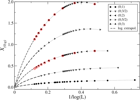
(b)

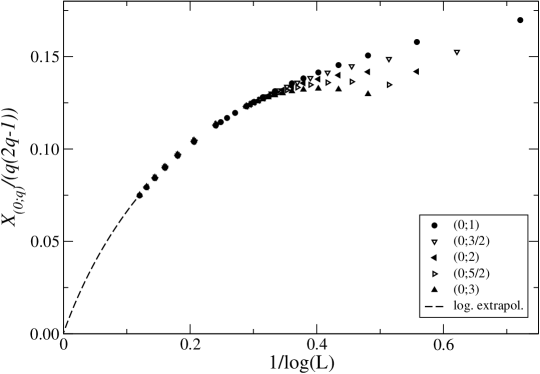
Figure 3: Scaling dimensions $X_{(0;q)}$ extracted from the finite-size behaviour of the energies of the lowest states in the sector $(0;q)$. These states have conformal spin $0$. Data obtained for the superspin chain with even (odd) number $L$ of sites are represented by filled (open) symbols. The dashed lines show the results of an extrapolation of the finite-size data (for system sizes up to $L=4096$) assuming a rational dependence on $1/\log L$, red circles indicate the results obtained within the string approximation (23)–(25). In (b) the data for the scaling dimensions are shown with the $X_{(0;q)}$ rescaled with the conjectured amplitude (21).

From these data we conclude that all dimensions $X_{(0;q)}$ with finite $q\geq 1$ vanish in the thermodynamic limit, showing subleading scaling corrections proportional to $1/\log L$. For $q>2$ the fact that $X_{(0;q)}\to 0$ can be obscured by the latter for quite large $L$ rendering a finite-size analysis based on small system sizes impossible.

To determine the amplitude of these subleading terms we note that this class of $(p=0;q)$-states can be extended to include the ground states of the superspin chain, i.e. the singlet $(0;0)$ for $L$ even and the quintet $(0,\frac{1}{2})$ for $L$ odd. Since there are no finite-size corrections to the energies of the ground states (with $q=0$ and $q=\frac{1}{2}$ for $L$ even and odd, respectively) we conjecture that the amplitudes of the logarithms are related to the quadratic Casimir (40) of $OSp(3|2)$ as

$$X_{(0;q)}=0+\frac{q(2q-1)}{\log(L/L_{0})}\,,\qquad q=0,\frac{1}{2},1,\frac{3}{2},2,\ldots$$ (21)

Comparing this conjecture with our numerical data we find very good agreement, see Figure 3(b). The lattice sizes $L$ considered here do not allow for a realiable estimate of the non-universal scale $\log L_{0}$ though. In the context of the loop model the amplitudes (21) determine the long distance asymptotics of the ’watermelon’ correlation functions $G_{k}(r)$ measuring the probability of $k$ loop segments connecting two points at distance $r$: these correlators – two-point functions of the so-called $k$-leg operators – vanish with a power of $1/\log r$, i.e.

$$G_{k}(r)\sim 1/\left(\log r\right)^{\alpha_{k}}\,.$$ (22)

The amplitudes conjectured for the periodic superspin chain imply that the exponents $\alpha_{k}$ are to be taken from the set $\{2q(2q-1),q=1,3/2,2,\ldots\}$, i.e. the eigenvalues of the quadratic Casimir (40) of $OSp(3|2)$. Identifying the $(0;q)$ primary with the $k=2q$-leg operator this agrees with RG calculations and numerical results for $G_{2}(r)$ and $G_{4}(r)$ Nahum et al. (2013). As will be seen below, however, the asymptotic behaviour of the watermelon correlators is likely to depend on the boundary conditions.

We further note that the reference state in the second Bethe ansatz is a highest weight state in the unique $(0;L/2)$ multiplet of the $OSp(3|2)$ superspin chain of length $L$. This indicates that the spectrum of the $(0;q)$ states considered here extends from the ground state energy $E_{0}=-3L$ to the energy $E(0;L/2)=-L$. This suggests that the critical dimensions (21) actually form a continuum starting at $X_{(0;0)}=0$. Additional support for this suggestion comes from the observation that for $q$ sufficiently large the imaginary parts of the Bethe roots in the $bfbfb$ grading are exponentially (in $L$) close to the hypothesis (19). In addition the real parts of the $(L-2q)/2$ pairs on each of the two levels take values very close to each other, i.e. $\mu_{j}^{(1)}\approx\mu_{j}^{(2)}$. In this situation the second set of the Bethe equations (16) is automatically satisfied while the first level ones become, after taking their logarithm,

$${L}\left[\psi_{5/4}(\mu_{j})-\psi_{1/4}(\mu_{j})\right]=-2\pi Q_{j}+\sum_{k\neq j}^{(L-2q)/2}\left[\psi_{3/2}(\mu_{j}-\mu_{k})+\psi_{1}(\mu_{j}-\mu_{k})-\psi_{1/2}(\mu_{j}-\mu_{k})\right]\,.$$ (23)

Here $\psi_{a}(x)=2\arctan(x/a)$ and the numbers $Q_{j}$ define the many possible branches of the logarithm being given by the expression,

$$Q_{j}=-\frac{1}{4}(L-2q)+j-\frac{1}{2},\quad j=1,\cdots,{\frac{1}{2}(L-2q)}\,.$$ (24)

Within this approach the eigenenergies corresponding to this state can be obtained using the following expression

$$E(\{\mu_{j}\})=-L+\frac{1}{2}\sum_{j=1}^{(L-2q)/2}\left[\frac{5}{(\mu_{j})^{2}+(5/4)^{2}}-\frac{1}{(\mu_{j})^{2}+(1/4)^{2}}\right]\,.$$ (25)

Comparing the numerical solution of these ’string’ equations with the those of (16) we conclude that the finite-size energies in the sectors $(0;q)$ with $q>2$ are reproduced by Eqs. (23)–(25), see Figure 3(a). In this formulation the root density approach can be applied to compute the finite-size energies. In this approach we find again that for $L\to\infty$ the conformal dimensions are zero, independent of $q$. This observation provides an additional analytical support to the existence of a continuum of zero conformal weights starting at zero.

V Other excitations

As for the sectors $(0;q)$ in the previous section we have identified the Bethe configurations corresponding to the lowest energy states in the sectors $(p;q)$ with $p\neq 0$. In Figure 4 we present the corresponding scaling dimensions for $p=1$.

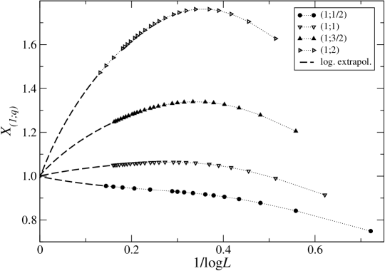
Figure 4: Same as Fig. 3(a) but now for the lowest states in the sector $(1;q)$. These states have conformal spin $1$.

Again, the energies show strong logarithmic corrections to scaling which are dealt with in the extrapolation by assuming a rational dependence of the finite-size data on $1/\log L$. For all states which we have considered the scaling dimension extrapolates to $X_{(1;q)}=1$. All of these states are found to carry momentum $\pm 2\pi/L$, from which we conclude that the corresponding fields have spin $1$.

The lowest energy levels in some sectors $(p;q)$ with $p>2$ are studied in an analogeous way, see Figures 5, 6, and 7.

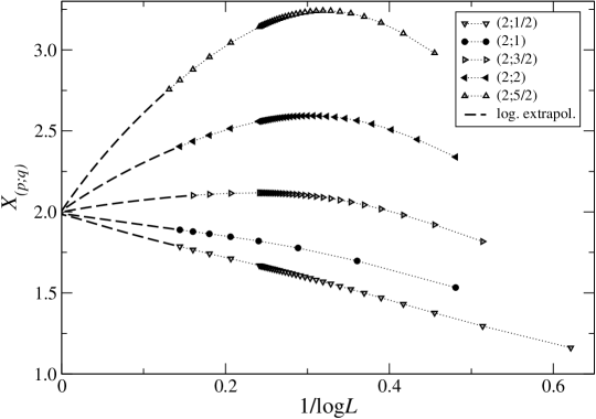
Figure 5: Same as Fig. 3(a) but now for the lowest states in the sector $(2;q)$. These states have conformal spin $0$.

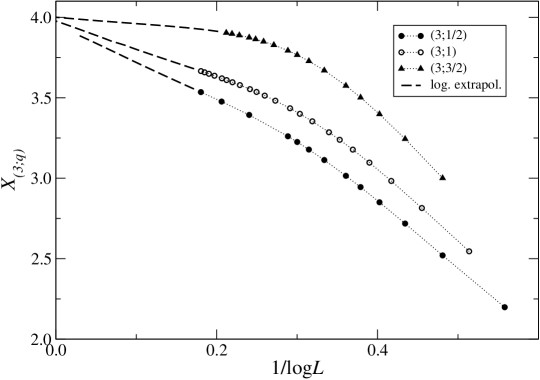
Figure 6: Same as Fig. 3(a) but now for the lowest states in the sector $(3;q)$. These states have conformal spin $2$.

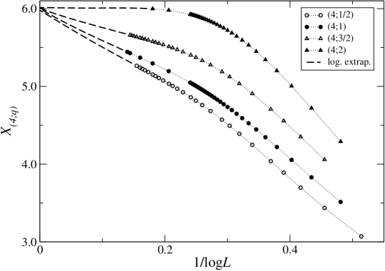
Figure 7: Same as Fig. 3(a) but now for the lowest states in the sector $(4;q)$. These states have conformal spin $0$.

The extrapolation gives scaling dimensions $X_{(2;q)}=2$, $X_{(3;q)}=4$, and $X_{(4;q)}=6$ as lower edges of continua of states with different $q$. The low lying states in sectors with $p=2,4$ have zero momentum while the states in the sectors $(3;q)$ have spin $2$. Note that the presence of these levels in the spectrum of the superspin chain of length $L$, requires the selection rule $L-p-2q\in 2\mathbb{N}$ to be satisfied.

In Table 1 we have collected the discrete parts of the conformal weights of primary operators in the CFT as identified from our numerical studies.

Table 1: Discrete part of the scaling dimensions $X$, conformal spin $s$ and corresponding conformal weights $(h,\bar{h})$ obtained from the lowest states observed in the symmetry sectors $(p;q)$ of the superspin chain.

sector $(p;q)$	$X=h+\bar{h}$	$s=h-\bar{h}$	$(h,\bar{h})$
$(0;q)$	$0$	$0$	$(0,0)$
$(1;q)$	$1$	$\pm 1$	$(1,0)$, $(0,1)$
$(2;q)$	$2$	$0$	$(1,1)$
$(3;q)$	$4$	$\pm 2$	$(3,1)$, $(1,3)$
$(4;q)$	$6$	$0$	$(3,3)$

Based on these data we conjecture that the spectrum of conformal weights is given by $h_{k}=\frac{1}{2}k(k+1)$, $k=0,1,2,\ldots$ and the lowest levels in the $(p;q)$ sector of the spectrum of the superspin chain correspond to operators with conformal weights

$$\left(h,\bar{h}\right)=\begin{cases}\left(h_{p/2},h_{p/2}\right)&\mathrm{for~{}}p\mathrm{~{}even}\,,\\ \left(h_{(p\pm 1)/2},h_{(p\mp 1)/2}\right)&\mathrm{for~{}}p\mathrm{~{}odd}\,.\end{cases}$$ (26)

Having identified the primary operators responsible for the lowest energy states we proceed to studying the finite-size behaviour of the other states appearing in the sector $(0;1)$: from the numerical diagonalization of the Hamiltonian (6) for the superspin chain with $L=6$ sites we observe, apart from the $(0;1)$ primary with vanishing scaling dimension (21), two low lying excitations with spin $\pm 1$ and three low lying excitations with zero spin. We have identified the configurations of Bethe roots corresponding to all of these except one of the spin $1$ states. Solving the Bethe equations for these configurations for larger system sizes and computing the corresponding scaling dimensions we find that they extrapolate to $X=2$ for two of the spin $0$ states, indicating a descendent field of the $(0;1)$ primary operator. The scaling dimensions of the third spin $0$ state and the spin $1$ state, however, do not converge to a finite value under extrapolation assuming a rational dependence on $1/\log L$ but rather disappear from the low energy spectrum, see Figure 8.

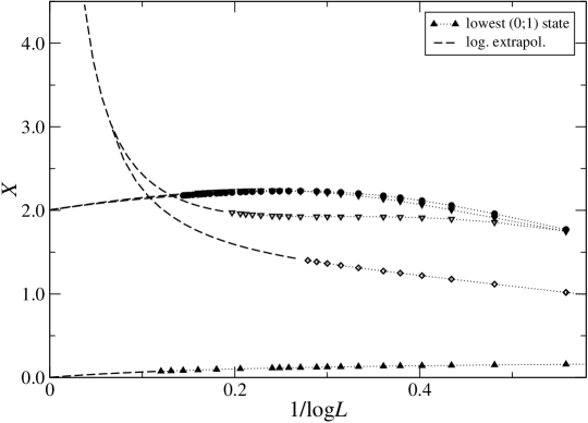
Figure 8: Scaling dimensions $X$ extracted from the finite-size behaviour of the energies of some low lying states in the $(0;1)$ sector together with their extrapolation assuming a rational dependence on $1/\log L$. The levels with $X\sim 1$ ($1.75$) for small systems (largest $1/\log L$) have conformal spin $1$ and $0$, respectively.

This behaviour is not limited to excitations in the $(0;1)$ sector but we have found such levels in many other sectors, too. Let us note that the removal of low energy states present in small systems in the scaling limit has also been observed in one phase of the $U_{q}[sl(2|1)]$ staggered superspin chain Frahm and Martins (2012). It is a direct consequence of the vanishing of a coupling constant, such as in (20) for the $OSp(3|2)$ model, and therefore expected to be a generic property of realizations for field theories with a continuous spectrum of critical exponents as lattice models with a compact quantum space.

From conformal field theory one expects a spin $1$ descendent of the $(0;1)$ primary field with scaling dimension $X=1$. This might be the other low energy spin $1$ level observed in the $L=6$ spectrum. Since we have not able to identify a solution to the Bethe equations (13) or (16) reproducing the numerical value for the energy, we cannot confirm this expectation.

VI Boundary Conditions

Here we would like to point out that peculiar finite-size behavior reported so far is also present if we had modified the boundary conditions such that the five possible states on the bonds of the vertex model are considered to be bosonic degrees of freedom. In this situation the vertex model transfer matrix is given, instead of (5), as the standard trace over the auxiliary space of the following product of operators,

$$\bar{{T}}(\lambda)=\sum_{a=1}^{5}\left[\bar{{I}}_{0{L}}{R}_{0{L}}(\lambda)\bar{{I}}_{0{L}-1}{R}_{0{L}-1}(\lambda)\cdots\bar{{I}}_{01}{R}_{01}(\lambda)\right]_{aa}$$ (27)

where the operator $\bar{{I}}_{0,j}=\sum_{a,b=1}^{5}(-1)^{p_{a}p_{b}}e_{aa}^{(0)}\times e_{bb}^{(j)}$ plays the role of a graded identity matrix. We recall here that this type of transfer matrix has been considered before in the case a vertex model based on the ${OSp}(1|2)$ superalgebra Martins (1995).

From the point of view of the spin chain this modification corresponds to imposing anti-periodic boundary for the fermionic degrees of freedom which splits the $(p;q)$ multiplets of the superspin chain into two subsets $(p;q)_{e}$ and $(p;q)_{o}$ containing states with even and odd number of fermions, respectively. In the Bethe equations this twist is reflected by additional phase factors depending on the sector label of the conserved charges. In the ${fbbbf}$ grading only the first set of the Bethe equations (13) is affected by this change of boundary conditions giving

$$\left[\frac{\lambda_{j}^{(1)}+i/2}{\lambda_{j}^{(1)}-i/2}\right]^{{L}} =(-1)^{n_{1}+1}\prod_{k=1}^{{L-n_{1}-n_{2}}}\frac{\lambda_{j}^{(1)}-\lambda_{k}^{(2)}+i/2}{\lambda_{j}^{(1)}-\lambda_{k}^{(2)}-i/2},\quad j=1,\cdots,{L-n_{1}},$$ (28)

$$\prod_{k=1}^{{L-n_{1}}}\frac{\lambda_{j}^{(2)}-\lambda_{k}^{(1)}+i/2}{\lambda_{j}^{(2)}-\lambda_{k}^{(1)}-i/2} =\prod_{k\neq j}^{{L-n_{1}-n_{2}}}\frac{\lambda_{j}^{(2)}-\lambda_{k}^{(2)}+i/2}{\lambda_{j}^{(2)}-\lambda_{k}^{(2)}-i/2},\quad j=1,\cdots,{L-n_{1}-n_{2}}\,.$$

The corresponding energies of the Hamiltonian with these boundary conditions are given by Eq. (12), as before.

It is evident from this construction that the finite-size spectrum will be different from that of the superspin chain only for sectors where the number of fermions $n_{1}$ is even. To see the effect on the scaling dimensions we have to take into account that the Bethe state of highest weight in the even fermion sector of the $(p;q)$-multiplet is parametrized by

$$n_{1}=p\,,\quad n_{2}=2q$$ (29)

rapidities in (28) for $p$ even rather than (10) which still holds for $p$ odd.

The ground state of the spin chain with twist is the unique singlet $(0;0)$ as for the superspin chain before. The corresponding root configuration consists of $L/2$ pairs of rapidities (17). Unlike the situation in the superspin chain the ground state of the twisted model has a strong finite-size dependence on $L$, see Figure 9(a):

Figure 9: (a) Central charge $c$ and (b) scaling dimensions $X$ extracted from the finite-size behaviour of the energies of the ground state and some low lying states $(p;q)_{e}$ with even fermion number of the spin chain subject to anti-periodic boundary conditions for the fermionic degrees of freedom. Dot-dashed lines in (b) indicate scaling dimensions extracted from the corresponding levels $(p;q)_{o}$ with an odd number of fermions.

the additional phase in the Bethe equations (28) leads to a central charge $c=3$ as noted before in Refs. Martins et al., 1998; Jacobsen et al., 2003. In addition there are subleading corrections to scaling which turn out to much stronger than the $1/[\log{L}]^{3}$ behavior usually observed in isotropic spin chains. We stress that this is even in contrast to the finite-size behavior found for other spin chains invariant by superalgebra such as ${OSp}(1|2)$ and ${OSp(2|2)}$.

In addition we have solved Eqs. (28) for some low energy excitations $(p;q)_{e}$ with even fermion number $n_{1}$. Their root configuration contains $n_{2}$ real roots $\lambda^{(1)}$ in addition to pairs as in the ground state. Our results show that the low energy spectrum of the spin chain with anti-periodic boundary conditions for the fermionic states shows a similar behaviour similar to that of the superspin chain, see Figure 9(b): the lowest excitations have fermion number $n_{1}=0$ with a continuous spectrum starting at scaling dimension $X_{e}=0$. As discussed above, the energies of states with odd fermion $n_{1}$ number are parametrized by the same rapidities as the corresponding $(p;q)$ multiplet of the superspin chain. Here the scaling dimensions, however, have to be computed from (18) relative to the new ground state which leads to a shift $X_{o}=X_{(p;q)}+c/12$ as a consequence of the different effective central charge. As in the superspin chain the subleading corrections to the scaling dimensions vanish as $1/\log L$. The amplitudes of these terms display a $q$-dependence which is clearly different from (21), even for the $X_{o}$ as a consequence of the logarithmic corrections to the central charge. Our data do not allow to quantify these amplitudes though: (much) larger system sizes would be needed for an estimate which is beyond the methods used in this work.

Appendix A Correspondence between the braid-monoid and the superalgebra realization of the intersecting loop model

The scattering rules of the Lorentz lattice gas and the configurations of the intersecting loop are algebraically realized in terms of the generators of a braid-monoid algebra first introduced by Brauer Brauer (1937). The braids $\mathrm{B}_{j}$ correspond to the right mirrors, the monoids $\mathrm{E}_{j}$ represent the left mirrors while the identity $\mathrm{I}_{j}$ describes the absence of a scatterer. These operators acts on the sites $j=1,\cdots,L$ of chain of length $L$ and satisfy a number of algebraic constraints:

• Braid relations

  $$\mathrm{B}_{j}\mathrm{B}_{j\pm 1}\mathrm{B_{j}}=\mathrm{B}_{j\pm 1}\mathrm{B}_{j}\mathrm{B}_{j\pm 1},~{}~{}\mathrm{B}_{j}^{2}=\mathrm{I}_{j},~{}~{}\mathrm{B}_{j}\mathrm{B}_{k}=\mathrm{B}_{k}\mathrm{B_{j}}~{}~{}\mbox{for}\hskip 8.5359pt|j-k|\geq 2$$ (30)

• Monoid relations

  $$\mathrm{E}_{j}\mathrm{E}_{j\pm 1}\mathrm{E}_{j}=\mathrm{E}_{j},~{}~{}\mathrm{E}_{j}^{2}=z\mathrm{E}_{j},~{}~{}\mathrm{E}_{j}\mathrm{E}_{k}=\mathrm{E}_{k}\mathrm{E}_{j}~{}~{}\mbox{for}\hskip 8.5359pt|j-k|\geq 2$$ (31)

  where ${z}$ is a free parameter representing the fugacity in the loop model version.

• Mixed relations

  $$\mathrm{B}_{j}\mathrm{E}_{j}=\mathrm{E}_{j}\mathrm{B}_{j}=\mathrm{E}_{j},~{}~{}\mathrm{E}_{j}\mathrm{B}_{j\pm 1}\mathrm{B}_{j}=\mathrm{B}_{j\pm 1}\mathrm{B}_{j}\mathrm{E}_{j\pm 1}=\mathrm{E}_{j}\mathrm{E}_{j\pm 1}$$ (32)

This algebra admits the construction of a one parameter family of integrable models by means of the approach known as Baxterization Jones (1990). The respective ${R}$-matrix is built out in terms of a weighted linear combination of the generators,

$${R}_{j}=w_{3}\,\mathrm{I}_{j}+w_{2}\,\mathrm{E}_{j}+w_{1}\,\mathrm{B}_{j}\,.$$ (33)

It turns out that the matrix ${R}_{j}$ fulfills the Yang-Baxter equation provided that the weights $w_{1}$, $w_{2}$ and $w_{3}$ are sited on the projective quadric,

$$(w_{1}+w_{2})w_{3}-\frac{2-z}{2}w_{1}w_{2}=0\,.$$ (34)

This manifold can be parameterized with the help of one spectral parameter $\lambda$ as follows,

$$w_{1}=w_{0}\,,\quad w_{2}=\frac{w_{0}\lambda}{1-z/2-\lambda}\,,\quad w_{3}=w_{0}\lambda$$ (35)

where $w_{0}$ is an overall normalization. Note that this factor can be chosen such that the weights configurations are interpreted as probabilities, i.e. $w_{0}=(z-2+2\lambda)/((z-2)(1+\lambda)+2\lambda^{2})$.

It has been observed Martins et al. (1998) that for integer $z$ this algebra has a realization in terms of a finite dimensional representation of the superalgebra $OSp({m}|2{n})$ provided that

$$z={m}-2{n}\,.$$ (36)

In this formulation the braid operator becomes the graded permutation between ${m}$ bosonic and $2{n}$ fermionic degrees of freedom,

$$\mathrm{B}_{j}=\sum_{a,b=1}^{{m}+2{n}}(-1)^{p_{a}p_{b}}e_{ab}^{(j)}\otimes e_{ba}^{(j+1)}\,,$$ (37)

where $p_{a}$ is the Grassmann parity of the $a$-th degree of freedom assuming values $p_{a}=0$ for bosons and $p_{a}=1$ for fermions.

Similarly, the monoid operator can be written as,

$$\mathrm{E}_{j}=\sum_{a,b,c,d=1}^{{m}+2{n}}\alpha_{ab}\alpha^{-1}_{cd}e_{ac}^{(j)}\otimes e_{bd}^{(j+1)}$$ (38)

where the matrix elements $\alpha_{ab}$ are

$$\alpha_{ab}=\begin{cases}{}(-1)^{1-{p_{a}}}\quad\mathrm{for~{}}a=b\cr+1\quad\mathrm{for~{}}a<b\mathrm{~{}with~{}}p_{a}=p_{b}=1\mathrm{~{}and~{}}\displaystyle\sum_{k=a+1}^{b}={n}\cr-1\quad\mathrm{for~{}}a>b\mathrm{~{}with~{}}p_{a}=p_{b}=1\mathrm{~{}and~{}}\displaystyle\sum_{k=b+1}^{a}={n}\cr 0\quad\mathrm{otherwise}\cr\end{cases}$$ (39)

in terms of the gradings $p_{a}$.

We remark that for some specific grading ordering the matrix $\alpha$ can be transformed into a block anti-diagonal structure. For a generic example see Ref. Martins and Ramos, 1997 and the main text, Eq. (4), for the case of $OSp(3|2)$.

Appendix B Finite dimensional representations of $OSp(3|2)$

As a consequence of the algebra inclusion $OSp(3|2)\supset SU(2)\oplus SU(2)$ one can use the labels of $SU(2)\oplus SU(2)$ irreps to classify the basis states of an $OSp(3|2)$ irrep, see der Jeugt (1984): except for the trivial representation $(0;0)$ the latter are characterized by two integer or half integer numbers $(p\geq 0;q\geq\frac{1}{2})$. The quadratic and quartic Casimir operators of $OSp(3|2)$ in terms of these numbers are

$$I_{2}=(p(p+1)+2q(1-2q))\,,\qquad I_{4}=\frac{1}{4}I_{2}\,(3p(p+1)+2(q+1)(2q-3))\,.$$ (40)

For example, the five-dimensional fundamental representation $(0;\frac{1}{2})$ of $OSp(3|2)$ carried by the local spins in the superspin chain decomposes as

$$(0;\frac{1}{2})=(1\otimes 0)\oplus(0\otimes\frac{1}{2})$$ (41)

into $(\ell\otimes s)$-representations of $SU(2)\oplus SU(2)$. States with integer (half-integer) spin in the second factor are bosonic (fermionic). Similarly, the first few of the other $OSp(3|2)$-representations with integer $p$ (i.e. the only ones relevant for the $OSp(3|2)$ superspin chain) can be decomposed as

$$(0;1) =(0\otimes 1)\oplus(1\otimes 0)\oplus(1\otimes\frac{1}{2})\,,$$ (42)

$$(0;q>1) =(0\otimes q)\oplus(1\otimes q-1)\oplus(1\otimes q-\frac{1}{2})\oplus(0\otimes q-\frac{3}{2})\,,$$

$$(p\geq 1;\frac{1}{2}) =(p-1\otimes 0)\oplus(p+1\otimes 0)\oplus(p\otimes\frac{1}{2})\,,$$

$$(1;1) =(1\otimes 1)\oplus(2\otimes 0)\oplus(1\otimes\frac{1}{2})\oplus(2\otimes\frac{1}{2})\,,$$

$$(p>1;1) =(p\otimes 0)\oplus(p\otimes\frac{1}{2})\oplus(p\otimes 1)\oplus(p-1\otimes 0)\oplus(p+1\otimes 0)$$

$$\qquad\oplus(p-1\otimes\frac{1}{2})\oplus(p+1\otimes\frac{1}{2})\,,$$

For $p\geq 1$ and $q\geq\frac{3}{2}$ with $p\neq 2q-1$ the “typical” $OSp(3|2)$-representation $(p;q)$ has dimension $4(2p+1)(4q-1)$ and is an eightfold pattern in the $SU(2)\oplus SU(2)$ decomposition

$$(p;q) =(p\otimes q)\oplus(p\otimes q-\frac{1}{2})\oplus(p-1\otimes q-\frac{1}{2})\oplus(p+1\otimes q-\frac{1}{2})$$ (43)

$$\qquad\oplus(p\otimes q-1)\oplus(p-1\otimes q-1)\oplus(p+1\otimes q-1)\oplus(p\otimes q-\frac{3}{2})\,.$$

For $p=2q-1$ some of the matrix elements of the $OSp(3|2)$ generators vanish which allows to decompose (43) into two “atypical” representations with a fourfold $SU(2)\oplus SU(2)$ decomposition

$$(p;q\equiv\frac{1}{2}(p+1))=(p\otimes q)\oplus(p\otimes q-\frac{1}{2})\oplus(p+1\otimes q-\frac{1}{2})\oplus(p+1\otimes q-1)\,.$$ (44)

Note that the atypical representations together with the irreps $(0;\frac{1}{2})$, $(1;1)$ and the trivial representation $(0;0)$ cannot be uniquely specified by the eigenvalues of the Casimir invariants (40): for all of them $I_{2}=I_{4}=0$. Therefore, they can appear as parts of reducible but indecomposable representations of $OSp(3|2)$ which are present in the spectrum of the superspin chain as will be discussed below.

Based on these relations the Hilbert space of the isotropic $OSp(3|2)$ superspin chain for small $L$ can be decomposed into $OSp(3|2)$-multiplets

$$(0;\frac{1}{2})^{\otimes 2} =(0;0)\oplus(0;1)\oplus(1;\frac{1}{2})\,,$$ (45)

$$(0;\frac{1}{2})^{\otimes 3} =(0;\frac{1}{2})\oplus(0;\frac{3}{2})\oplus(2;\frac{1}{2})\oplus 2*\left[2*(0;\frac{1}{2})\oplus(1;1)\right]_{\mathrm{ind}}\,,$$

$$(0;\frac{1}{2})^{\otimes 4} =(0;0)\oplus 6*(0;1)\oplus(0;2)\oplus 6*(1;\frac{1}{2})\oplus 3*(1;\frac{3}{2})$$

$$\quad\oplus 3*(2;1)\oplus(3;\frac{1}{2})\oplus 2*\left[2*(0;0)\oplus(1;1)\right]_{\mathrm{ind}}\,.$$

By $\left[\ldots\right]_{\mathrm{ind}}$ we denote the combinations of atypical representations in reducible but indecomposable ones. The decompositions (45) have been checked numerically. Note that the trivial and the fundamental representation of $OSp(3|2)$ appear exactly once in the tensor product for even and odd $L$, respectively. Furthermore, all other multiplets appearing in (45) have even dimension and contain the same number of bosonic and fermionic states. This leads to the trivial partition function (7) of the $OSp(3|2)$ vertex model.

Reference states to be used in the algebraic Bethe ansatz of the superspin chain with $L>1$ sites, each carrying the representation (41), can be highest weight states of (either of) the $(8L-4)$-dimensional multiplets $(L-1;\frac{1}{2})$ or $(0;\frac{1}{2}L)$.

References

- Martins et al. (1998) M. J. Martins, B. Nienhuis, and R. Rietman, “An Intersecting Loop Model as a Solvable Super Spin Chain,” Phys. Rev. Lett. 81, 504–507 (1998), cond-mat/9709051 .
- Ruijgrok and Cohen (1988) Th. W. Ruijgrok and E. G. D. Cohen, “Deterministic lattice gas models,” Phys. Lett. A 133, 415–418 (1988).
- Gunn and Ortuño (1985) J. M. F. Gunn and M. Ortuño, “Percolation and motion in a simple random environment,” J. Phys. A 18, L1095–L1101 (1985).
- Ziff et al. (1991) Robert M. Ziff, X. P. Kong, and E. G. D. Cohen, “Lorentz lattice-gas and kinetic-walk model,” Phys. Rev. A 44, 2410–2428 (1991).
- Owczarek and Prellberg (1995) A. L. Owczarek and T. Prellberg, “The collapse point of interacting trails in two dimensions from kinetic growth simulations,” J. Stat. Phys. 79, 951–967 (1995).
- Cao and Cohen (1997) Meng-She Cao and E. G. D. Cohen, “Scaling of particle trajectories on a lattice,” J. Stat. Phys. 87, 147–178 (1997).
- Jacobsen et al. (2003) J. L. Jacobsen, N. Read, and H. Saleur, “Dense Loops, Supersymmetry, and Goldstone Phases in Two Dimensions,” Phys. Rev. Lett. 90, 090601 (2003), cond-mat/0205033 .
- Essler et al. (2005) Fabian H. L. Essler, Holger Frahm, and Hubert Saleur, “Continuum limit of the integrable - superspin chain,” Nucl. Phys. B 712 [FS], 513–572 (2005), cond-mat/0501197 .
- Frahm and Martins (2011) Holger Frahm and Márcio J. Martins, “Finite size properties of staggered superspin chains,” Nucl. Phys. B 847, 220–246 (2011), arXiv:1012.1753 .
- Vernier et al. (2014) Éric Vernier, Jesper Lykke Jacobsen, and Hubert Saleur, “Non compact conformal field theory and the (Izergin-Korepin) model in regime III,” J. Phys. A 47, 285202 (2014), arXiv:1404.4497 .
- Frahm and Martins (2012) Holger Frahm and Márcio J. Martins, “Phase Diagram of an Integrable Alternating Superspin Chain,” Nucl. Phys. B 862, 504–552 (2012), arXiv:1202.4676 .
- Ikhlef et al. (2008) Yacine Ikhlef, Jesper Lykke Jacobsen, and Hubert Saleur, “A staggered six-vertex model with non-compact continuum limit,” Nucl. Phys. B 789, 483–524 (2008), cond-mat/0612037 .
- Ikhlef et al. (2012) Yacine Ikhlef, Jesper Lykke Jacobsen, and Hubert Saleur, “An integrable spin chain for the SL(2,R)/U(1) black hole sigma model,” Phys. Rev. Lett. 108, 081601 (2012), arXiv:1109.1119 .
- Candu and Ikhlef (2013) Constantin Candu and Yacine Ikhlef, “Non-Linear Integral Equations for the SL(2,R)/U(1) black hole sigma model,” J. Phys. A 46, 415401 (2013), arXiv:1306.2646 .
- Frahm and Seel (2014) Holger Frahm and Alexander Seel, “The staggered six-vertex model: Conformal invariance and corrections to scaling,” Nucl. Phys. B 879, 382–406 (2014), arXiv:1311.6911 .
- Kager and Nienhuis (2006) Wouter Kager and Bernard Nienhuis, “Monte Carlo study of the hull distribution for the q=1 Brauer model,” J. Stat. Mech. , P08004 (2006), cond-mat/0606370 .
- Nahum et al. (2013) Adam Nahum, P. Serna, A. M. Somoza, and M. Ortuño, “Loop models with crossings,” Phys. Rev. B 87, 184204 (2013), arXiv:1303.2342 .
- Martins and Ramos (1997) M. J. Martins and P. B. Ramos, “The algebraic Bethe ansatz for rational braid-monoid lattice models,” Nucl. Phys. B 500, 579–620 (1997), hep-th/9703023 .
- Alcaraz and Martins (1990) Francisco Castilho Alcaraz and Marcio Jose Martins, “The spin-S XXZ quantum chain with general toroidal boundary conditions,” J. Phys. A 23, 1439–1451 (1990).
- Yang and Yang (1969) C. N. Yang and C. P. Yang, “Thermodynamics of a one-dimensional system of bosons with repulsive delta-function interaction,” J. Math. Phys. 10, 1115–1122 (1969).
- Blöte et al. (1986) H. W. J. Blöte, John L. Cardy, and M. P. Nightingale, “Conformal invariance, the central charge and universal finite-size amplitudes at criticality,” Phys. Rev. Lett. 56, 742–745 (1986).
- Affleck (1986) Ian Affleck, “Universal term in the free energy at a critical point and and the conformal anomaly,” Phys. Rev. Lett. 56, 746–748 (1986).
- Polyakov (1975) A. M. Polyakov, “Interaction of goldstone particles in two dimensions. Applications to ferromagnets and massive Yang-Mills fields,” Phys. Lett. B 59, 79–81 (1975).
- Read and Saleur (2001) N. Read and H. Saleur, “Exact spectra of conformal supersymmetric nonlinear sigma models in two dimensions,” Nucl. Phys. B 613, 409–444 (2001), hep-th/0106124 .
- Martins (1995) M. J. Martins, “The exact solution and the finite-size behaviour of the -invariant spin chain,” Nucl. Phys. B 450, 768–788 (1995), hep-th/9502133 .
- Brauer (1937) Richard Brauer, “On Algebras Which are Connected with the Semisimple Continuous Groups,” Ann. Math. 38, 857–872 (1937).
- Jones (1990) V. F. R. Jones, “Baxterization,” Int. J. Mod. Phys. B 4, 701–713 (1990).
- der Jeugt (1984) Joris Van der Jeugt, “Finite- and infinite-dimensional representations of the orthosymplectic superalgebra OSP(3,2),” J. Math. Phys. 25, 3334–3349 (1984).