Counter-ion density profile around a charged disk: from the weak to the strong association regime

Abstract

We present a comprehensive study of the two dimensional one component plasma in the cell model with charged boundaries. Starting from weak couplings through a convenient approximation of the interacting potential we were able to obtain an analytic formulation to the problem deriving the partition function, density profile, contact densities and integrated profiles that compared well with the numerical data from Monte-Carlo simulations. Additionally, we derived the exact solution for the special cases of $\Xi=1,2,3,\dots$ finding a correspondence between those from weak couplings and the latter. Furthermore, we investigated the strong coupling regime taking into consideration the Wigner formulation. Elaborating on this, we obtained the profile to leading order, computed the contact density values as compared to those derived in an earlier work on the contact theorem. We formulated adequately the strong coupling regime for this system that differed from previous formulations. Ultimately, we calculated the first order corrections and compared them against numerical results from our simulations with very good agreement; these results compared equally well in the planar limit, whose results are well known.

I Introduction

In this work we present a thorough analysis of the condensation phenomenon of counter-ions around a charged disk. The model under consideration is a two-dimensional (2D) system formed by an impenetrable disk of charge $Q_{1}$ surrounded by ions dispersed freely in a larger disk with external charged boundary $Q_{2}$ and no dielectric discontinuities between the regions delimited by the geometry. The problem resembles an annulus with particles moving freely between the inner and outer radii as in fig. 1. The $N$ ions have, respectively, a charge $-q$ in such a way that neutrality yields,

$$Q_{1}+Q_{2}=N\,q.$$ (1)

We will assume a point-like geometry for the free charges, which is not a problem due to electrostatic repulsion alone. This model is seemingly the one component plasma (2D-OCP) with a small variation. First the neutralizing charge is not distributed homogeneously in the background and second the inner core is impenetrable.

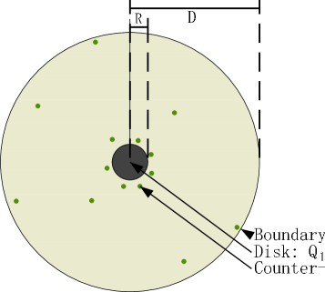
Figure 1: The 2D cylindrical cell model. The disk with charge $Q_{1}$ and radius $R$ is surrounded by counter-ions with charge $-q$ within $R$ and the external boundary at $D$ with charge $Q_{2}$. The interior of the disk and the exterior of the cell have the same dielectric material.

This is the two-dimensional analog of the Manning counter-ion condensation phenomenon around charged cylinders Manning (1969b, c, a). Unlike the three-dimensional (3D) situation where the Coulomb potential shapes as $1/\left|\mathbf{r}\right|$, the partition function for two-dimensional Coulomb systems is written as a product of contributions which, in some cases, may be computed exactly. That and the logarithmic nature of the potential motivated the theoretical computation of the abundant static and dynamic properties of electrolytes for two-dimensional systems.

The interaction between two unit charges separated by a distance $r$ is given by the two-dimensional Coulomb potential $-\log(r/L)$, where $L$ is an irrelevant arbitrary length scale. We are interested in the equilibrium thermal properties of the system at a temperature $T$. As usual, we define $\beta=1/(k_{B}T)$ where $k_{B}$ is the Boltzmann constant. There are three important dimensionless parameters which caracterize the system. The 2D equivalent of the Manning parameter is $\xi=\beta qQ_{1}/2$, which caracterizes the strengh of the Coulomb coupling between the inner disk and the counter-ions. The Coulomb coupling between counter-ions is $\Xi=\beta q^{2}/2$. Here the familiarized reader may have noticed that for the two dimensional systems it is accustomed to use $\Gamma$ for the notation of the coupling constant Šamaj et al. (1994); Téllez and Forrester (1999); Forrester et al. (1983); Forrester (1985); Cornu and Jancovici (1989); the previous defined coupling equates the standardized one as $\Xi=\Gamma/2$, but we have kept $\Xi$ motivated by a discussion with the three dimensional case. Finally the third parameter, defined as $\Delta=\log(D/R)$, which measures in log-scale the size of the system.

To our problem, we acknowledge the published works from Naji and Netz (2005, 2006) and Burak and Orland (2006), which have covered thoroughly the basics of the two dimensional construction of the cell model. They observed that condensation obeys the well-known threshold at $\xi=1$ where below this value there is none. In mean field, it is known that a disk or cylinder with a dimensionless charge inferior to unity is unable to bind counter-ions. When the charge is above unity, it attracts an ion cloud in such a way that it neutralizes partially the disk/cylinder so that the effective dimensionless charge of the disk/cylinder and the cloud is unity. Hence, the fraction of condensed ions in the cloud corresponds to the excess above unity by the total, also known as the Manning fraction $f_{M}=1-1/\xi$. They also showed that the system with two dimensions differs from the three-dimensional one in several ways. First of all, when the outer boundary is uncharged $Q_{2}=0$, the relationship between the coupling parameter and the Manning parameter is dictated by neutrality, which, unlike in 3D where they both enjoyed independence, it fixes one or the other in such a way that,

$$\Xi\,=\,\xi/N,$$ (2)

as will be discussed in section II.

Additionally, if we were to look at a system with a fixed number of particles going from a temperature above the critical temperature for condensation, i.e. $\xi<1$, and allow it undergo a cooling process, the energy, heat capacity and other quantities will present successive transitions due to iterative localization phenomena occurring when a counter-ion is condensed Naji and Netz (2005, 2006); Burak and Orland (2006).

The interesting regime for the two dimensional construction is that which corresponds to small number of counter-ions. Due to eq. 2, a large number $N$ of ions is equivalent to $\Xi\to 0$ which is unquestionably the mean field regime. Therefore, as mentioned before by Naji and Netz (2005), our interest stands in the range for weak and strong couplings controlled by the ratio between $\xi$ and the number of counter-ions.

The outline for the following work begins with the presentation of the two dimensional model (Sec. II), followed in Sec. III by an analysis of the regime when $\Xi<1$ (or $\Gamma<2$), where we extend previous works by Burak and Orland (2006); Naji and Netz (2005, 2006); Varghese et al. (2012). Then follows, in Secs. IV and V, the study of the special cases $\Xi=1,2,3,\dots$ (or $\Gamma=2,4,6,\dots$), which are exactly solvable using expansions of powers of Vandermonde determinants in basis of symmetric or antisymmetric monomials (Šamaj et al., 1994; Téllez and Forrester, 1999; Šamaj, 2004; Téllez and Forrester, 2012). Through these analytic models we will be able to obtain the profiles and the energy along with all the quantities associated with them. Furthermore, we will present a model for condensation in each case.

Finally, we study, in Sec. VI, the strong coupling situation when $\Xi\gg 1$ (or $\Gamma\gg 2$) with special attention to condensation and evaluate the profile and other statistical properties. Ultimately, we will retake the contact theorem to obtain the value of the densities at contact comparing to the values derived by the models and numerical Monte Carlo simulations.

II The model

The Hamiltonian for the system considering the logarithmic Coulomb potential interaction between charges as the solution to the Poisson equation $\nabla_{\mathbf{r}}^{2}v(\mathbf{r})=2\pi\delta(\mathbf{r})$ reads as,

$$\mathcal{H}\mathrel{\mathop{:}}=\beta H= \beta Q_{1}q\sum_{j=1}^{N}\log\frac{|\mathbf{r}_{j}|}{L}+N\beta Q_{2}q\log\frac{D}{L}-\beta q^{2}\sum_{1\leq j<k\leq N}\log\left|\frac{\mathbf{r}_{j}-\mathbf{r}_{k}}{L}\right|$$ (3)

$$-\beta Q_{1}Q_{2}\log\frac{D}{L}-\frac{\beta Q_{1}^{2}}{2}\log\frac{R}{L}-\frac{\beta Q_{2}^{2}}{2}\log\frac{D}{L},$$

where $L$ is an arbitrary reference length. The position vector, with respect to the center of the disk, of the particle number $j$ is denoted by $\mathbf{r}_{j}$. It will prove convenient to use polar coordinates $r_{j}=|\mathbf{r}_{j}|$ and $\theta_{j}$. Notice that due to Gauss’ theorem the contribution to the Hamiltonian of the exterior charge $Q_{2}$ interacting with $Q_{1}$ and counter-ions is independent of the positions, yielding a constant. For that matter, this system’s behavior depends on $Q_{1}-Nq$, which can take arbitrary values.

We may introduce the standardized dimensionless notation suggested by Naji and Netz (2006, 2005) by rescaling all distances with the Gouy-Chapmann length ($\mu=R/\xi$), i.e. $\widetilde{r}=r/\mu$, but this will only be important extending the analysis to the planar limit at which the Gouy length is significant; to this problem, all radial distances will be divided by either $R$ or $D$. Substituting the Manning parameter as $\xi=(\beta\,Q_{1}\,q/2)$ and the coupling $\Xi=\beta\,q^{2}/2$ (or $\Gamma=\beta q^{2}$) we obtain, using eq. 1,

$$\beta Q_{2}^{2}=2\frac{\left[N\Xi-\xi\right]^{2}}{\Xi}$$ (4)

$$\mathcal{H}= 2\xi\sum_{j=1}^{N}\log\left|\frac{\mathbf{r}_{j}}{R}\right|-2\Xi\sum_{1\leq j<k\leq N}\log\left|\frac{\mathbf{r}_{j}-\mathbf{r}_{k}}{R}\right|+E_{0},$$ (5)

where,

$$E_{0}=\frac{\left[N\Xi-\xi\right]^{2}}{\Xi}\Delta+N\Xi\log\frac{R}{L}\,=\,\frac{\xi_{B}^{2}}{\Xi}\Delta+N\Xi\log\frac{R}{L},$$ (6)

with $\xi_{B}$ a parameter equivalent to $\xi$ that speaks of the dimensionless charge accumulated in the exterior boundary. Neutrality reads then in terms of these set of parameters as,

$$\xi+\xi_{B}=N\Xi\quad\text{and}\quad\xi_{B}=\frac{Q_{2}}{Q_{1}}\xi.$$ (7)

A remarkable feature is the relationship, through neutrality with neutral exterior boundary, between the coupling and the number of particles in the absence of external charge ($Q_{2}=0$). Therefore, as in Naji and Netz (2005), we recover the mean field regime as $\Xi\to 0$ (or $\Gamma\to 0$) which amounts to say that $N\to\infty$ at constant $\xi$, as was shown by Burak and Orland (2006).

However, the situation for finite $N$ is quite different. Naji and Netz (2005) showed how the energy, heat capacity and the order parameter presented a series of transitions that were absent in the three dimensional case. The underpinnings of this process are at the condensation of ions when reducing the temperature.

In order to see this, we will investigate the problem in three phases. The first, we will focus on $\Xi<1$ (or $\Gamma<2$) through a method proposed by Burak and Orland (2006); Varghese et al. (2012). Then we will look at the integer $\Xi$ (or even $\Gamma$) cases which admit a analytic solutions as a prelude to the $\Xi>1$ case, or the strong coupling regime with some interesting features due to curvature.

In all the different coupling regimes considered, we will compare our analytical predictions to Monte Carlo simulation data, obtained with a code developped by one of the authors (JPM). The code uses the so-called centrifugal sampling Naji and Netz (2006), that uses $y=\log(r/R)$ as variable, necessary to sample large box sizes ($D\gg R$). Also, besides the usual Monte Carlo moves, the codes implements moves that exchanges particles between the condensed and un-condensed populations ($y\longmapsto\Delta-y$), necessary to properly sample the configuration space Mallarino et al. (2013). The ions are point-like particles of a single type in order to avoid the introduction of hard-core interactions. Considering ions with size is a perspective for a future work due to the non-trivial behavior emerging from steric effects. Regarding the sampling steps, data was collected after proper thermalization for as long as $10^{8}$ steps.

III The weakly coupled case or $\Xi<1$

Our analysis begins in the $\Xi<1$ case which is better recalled as the weakly coupled case. We indicated that $N\to\infty$ recovers mean field which is not particularly interesting. However, when the number of counter-ions is small and the coupling too, some interesting phenomena occur. This has been described before as a transition due to the condensation of an ion, which is not smooth as in the three dimensional case. In order to see this, let us evaluate the partition function $\mathcal{Z}(\Xi,\xi,N,\Delta)$ assuming that the box’s radius is much larger than that of the disk (large $\Delta$). Here, the logarithmic interaction term can be written conveniently (Burak and Orland, 2006; Varghese et al., 2012),

$$2\log|\mathbf{r}_{1}-\mathbf{r}_{2}|= \log\left\|\mathbf{r}_{1}\right\|+\log\left\|\mathbf{r}_{2}\right\|$$ (8)

$$+\log\left[2\cosh\left(\log\left\|\mathbf{r}_{1}\right\|-\log\left\|\mathbf{r}_{2}\right\|\right)-2\cos\theta_{12}\right],$$

where $\theta_{12}=\theta_{1}-\theta_{2}$. In the weakly coupled limit angular correlations are neglectible thus we can construct an effective interacting potential averaging over the angle in such a way that,

$$\left\{2\log|\mathbf{r}_{1}-\mathbf{r}_{2}|\right\}_{\text{eff}}\mathrel{\mathop{:}}=\frac{1}{2\pi}\int_{0}^{2\pi}2\log|\mathbf{r}_{1}-\mathbf{r}_{2}|\text{d}\theta=2\log\left|\mathbf{r}_{>}\right|,$$ (9)

where $\left|\mathbf{r}_{>}\right|\equiv\text{max}(\left|\mathbf{r}_{1}\right|,\left|\mathbf{r}_{2}\right|)$; consequently,

$$2\log|\mathbf{r}_{1}-\mathbf{r}_{2}|\simeq 2\log\left|\mathbf{r}_{>}\right|.$$ (10)

Keep in mind that this approximation is not valid for high couplings or small box sizes where angular correlations are not negligible (i.e. $D\to R$ would represent another problem, a ring of counter-ions in two dimensions). Under these assumptions, the Hamiltonian (5) reads,

$$\mathcal{H}\approx\frac{2\xi}{\Xi}\sum_{j=1}^{N}y_{j}-2\sum_{1\leq j<k\leq N}y_{>}^{(j,k)}+E_{0},$$ (11)

with $y_{j}=\Xi\log(r_{j}/R)$ and $y_{>}^{(j,k)}$ the greatest of $y_{j}$ and $y_{k}$. The partition function is then conveniently written in terms of the $\{y_{k}\}$ variables as,

$$\mathcal{Z}=\frac{1}{N!}\left(\frac{R^{2}}{\Xi}\right)^{N}\int\text{d}^{N}y\,\text{d}^{N}\theta\,e^{-\mathcal{H}+\frac{2}{\Xi}\sum_{j=1}^{N}y_{j}}.$$ (12)

Via the transformation of coordinates we redefine the energy $\mathcal{H}^{\prime}\mathrel{\mathop{:}}=\mathcal{H}-\frac{2}{\Xi}\sum_{j}y_{j}\,-E_{0}$ containing all the important behavior of the system. There is an analytic route to evaluate the partition function as commanded by Burak and Orland (2006). The following procedure follows closely that which was done by the abovementioned authors as part of the presentation of the problem in this context. In order to integrate the Boltzmann factor over the coordinate’s phase space we separate the intervals from least to greatest. We know that each partitioning of the phase space that is an ordered arrangement of the $\{y_{k}\}$’s corresponds to a simple permutation of the base order (denoted by [BO]): $y_{1}<y_{2}<\dots<y_{N}$. Then, eq. 12 yields,

$$\mathcal{Z}=e^{-E_{0}}\left(\frac{2\pi\,R^{2}}{\Xi}\right)^{N}\int_{0}^{\Xi\Delta}\text{d}y_{N}\int_{0}^{y_{N}}\text{d}y_{N-1}\dots\int_{0}^{y_{2}}\text{d}y_{1}\,e^{-\mathcal{H}^{\prime}}.$$ (13)

Burak et. al. realized that the Boltzmann factor could be written conveniently as a product of functions and the form of the integral involved is a successive convolution of functions. Using the Laplace transformation we can evaluate the partition function analytically. Arranging the set of $\{y_{j}\}$’s by the [BO] $\mathcal{H}^{\prime}$ reads in simplified form,

$$\mathcal{H}^{\prime}=\sum_{j=0}^{N}a_{j}(y_{j+1}-y_{j})-a_{N}\Xi\Delta=\sum_{j=1}^{N}(a_{j-1}-a_{j})y_{j},$$ (14)

where $y_{0}=0$ and $y_{N+1}=\Xi\Delta$, and the positive constants $\{a_{j}\}$ are conveniently defined as,

$$a_{j}=\left[j-\left(\frac{\xi-1}{\Xi}+\frac{1}{2}\right)\right]^{2}$$ (15)

$$a_{j-1}-a_{j}=2\frac{\xi-1}{\Xi}-2(j-1)$$

The choice for the set of $\{a_{j}\}$ is not unique since we have a total of $N+1$ variables and $N$ conditions; then an arbitrary choice for any term will define the rest. Anticipating the following steps, choosing each of the terms positive will be convenient in the calculation of the Laplace transformation of the partition function. Note that $a_{j}$ has a minimum sitting on

$$j_{\text{min}}=\sqrt{a_{0}}=\frac{\xi-1}{\Xi}+\frac{1}{2}\,,$$ (16)

thus telling that the smallest term of the set is that which $j$ is the integer closest to $j_{\text{min}}$.

Through this construction we are now able to evaluate the partition function writing the integral as a convolution of functions $\{f_{j}\}$. From eq. 13,

$$\mathcal{Z}= \left(\frac{2\pi\,R^{2}}{\Xi}\right)^{N}\,e^{a_{N}\Xi\Delta-E_{0}}$$ (17)

$$\times\int_{0}^{\Xi\Delta}\text{d}y_{N}\int_{0}^{y_{N}}\text{d}y_{N-1}\dots\int_{0}^{y2}\text{d}y_{1}\,\prod_{j=0}^{N}f_{j}\left(y_{j+1}-y_{j}\right)$$

$$= \left(\frac{2\pi\,R^{2}}{\Xi}\right)^{N}\,e^{a_{N}\Xi\Delta-E_{0}}\left[f_{N}\otimes f_{N-1}\otimes\cdots\otimes f_{1}\otimes f_{0}\right](\Xi\Delta),$$

with $f_{j}(x)=e^{-a_{j}x}$, whereas the Laplace transform of the convolution part is then,

$$\mathcal{T}_{\left\{f_{N}\otimes\cdots\otimes f_{0}\right\}}^{\left[\Xi\Delta\right]}(s)= \int_{0}^{\infty}\left[f_{N}\otimes f_{N-1}\otimes\cdots\otimes f_{1}\otimes f_{0}\right](\Xi\Delta)\,e^{-s(\Xi\Delta)}\text{d}(\Xi\Delta)$$ (18)

$$= \prod_{j=0}^{N}\frac{1}{s+a_{j}}$$

The milestone of this analysis is the approximation of the interacting potential term, valid for a large box size ($\Delta\gg 1$). A small box size surfaces other effects which cannot be neglected. The route of the simplification comes from transforming the two-dimensional gas into a one-dimensional mean interacting strip of ions (Burak and Orland, 2006).

As we proceed to invert the Laplace transform to obtain the partition function, factors of the form $e^{-a_{j}\Xi\Delta}$ will emerge in the function where the dominating contributions will come from the smallest of the $\{a_{j}\}$’s; this fact enforces choosing a positive value for $a_{j}$. Hence, the prevailing term is the smallest of the set, indicated by $j^{\star}$, and closest to $\sqrt{a_{0}}$, or,

$$j_{inf}^{\star}=\left\lfloor\frac{f_{M}N}{1+\frac{\xi_{B}}{\xi}}+\frac{1}{2}\right\rfloor \leq j^{\star}\leq\left\lceil\frac{f_{M}N}{1+\frac{\xi_{B}}{\xi}}+\frac{1}{2}\right\rceil=j_{sup}^{\star}.$$ (19)

However, choosing the lower or upper bounds depends if

$$a_{j_{inf}^{\star}}\leq a_{j_{sup}^{\star}}\,\,\Rightarrow\,\,j^{\star}=\left\lfloor\frac{f_{M}N}{1+\frac{\xi_{B}}{\xi}}+\frac{1}{2}\right\rfloor$$

$$a_{j_{inf}^{\star}}>a_{j_{sup}^{\star}}\,\,\Rightarrow\,\,j^{\star}=\left\lceil\frac{f_{M}N}{1+\frac{\xi_{B}}{\xi}}+\frac{1}{2}\right\rceil.$$

Since $j_{sup}^{\star}=j_{inf}^{\star}+1$ we can rewrite the previous condition using LABEL:eq:a_rec_rel in such a way that the sign of $\left((\xi-1)/\Xi-j_{inf}^{\star}\right)$ will determine the minimal parameter; a representation of this situation is given in fig. 2. We can summarize,

$$j^{\star}=\left\lfloor\frac{f_{M}N}{1+\frac{\xi_{B}}{\xi}}\right\rfloor+1.$$ (20)

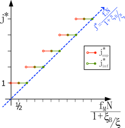
Figure 2: The value for $j^{\star}$ as a function of ${f_{M}N}/(1+\xi_{B}/\xi)$. Notice the solution is the composition of the red and the green parts which tells us that $j^{\star}=\left\lfloor{f_{M}N}/(1+\xi_{B}/\xi)\right\rfloor+1$ and signals the discontinuities precisely at the points where ${f_{M}N}/(1+\xi_{B}/\xi)$ is a whole number.

The mathematical relationship for $j^{\star}$ hides even so a more important fact about this particular system in relation to condensation. Inspecting the aforementioned equation, $N/(1+{\xi_{B}}/{\xi})$ corresponds to the number of counter-ions that neutralize the center disk charge (namely $N_{n}$); or, by using eq. 7, $N_{n}=\xi/\Xi=N-\xi_{B}/\Xi$ (i.e. $N_{n}=N-2\xi_{B}/\Gamma$). Furthermore, we know from previous works in mean field (Burak and Orland, 2006; Naji and Netz, 2005, 2006; Mallarino et al., 2013) that the ratio of condensed ions is the well-known Manning relationship $f_{M}$. In other words, from eq. 20,

$$\frac{j^{\star}}{N_{n}}\overset{N\to\infty}{=}f_{M},$$ (21)

thus recovering the celebrated Manning condensation fraction in the thermodynamic limit. As a result, $j^{\star}$ will be intrinsically related to the number of condensed ions; this will be further clarified in the following sections.

III.1 The partition function

In order to invert the transform for the partition function $\mathcal{Z}$ we need to revise three possible cases according to the set of $\left\{a_{j}\right\}$. These cases depend on the values of $\Xi$ and $\xi$. In fact, given that the $a_{j}=(j-c)^{2}$, with $c=\frac{\xi-1}{\Xi}+\frac{1}{2}$, the set will be degenerate if given two values $k$ and $j$, $a_{j}=a_{k}$. That is the case of either $j=k$ or that $2c\in\mathbb{Z}$. In other words, $c$ could be either a semi or a whole number. In terms of our variables $\xi$, $\xi_{B}$, $\Xi$ and $N$ it implies that

$$\frac{2}{\Xi}\left(1+\xi_{B}\right) \in\mathbb{N}$$ (22)

or

$$\frac{2}{\Xi}+2(N-N_{n}) \in\mathbb{N}$$

There are three cases that correspond to different kinds of solutions as follows:

1. The non-degenerate case

   

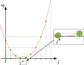
   Figure 3: Representation of $a_{j}$ as a function of $j$ with $j^{\star}$ the location of the minimum of the $\left\{a_{j}\right\}$ for the non-degenerate case

   For this case, the values of $a_{j}$ are non-degenerate as shown in fig. 3. Given that we expect a simple separation of the product terms from LABEL:eq:laplace_Z_simple into sums as,

   $$\mathcal{T}_{\left\{f_{N}\otimes\cdots\otimes f_{0}\right\}}^{\left[\Xi\Delta\right]}(s)= \prod_{k=0}^{N}\frac{1}{s+a_{k}}=\sum_{k=0}^{N}C_{k}\frac{1}{s+a_{k}},$$ (23)

   with coefficients $C_{k}=\prod_{l=0,l\neq k}^{N}\frac{1}{a_{l}-a_{k}}$ simplified to,

   $$C_{k}=\frac{2(-1)^{k}}{k!\left(N-k\right)!}\frac{\left(k-\left[\frac{\xi-1}{\Xi}+\frac{1}{2}\right]\right)\,\mathbf{\Gamma}\left(k-2\left[\frac{\xi-1}{\Xi}+\frac{1}{2}\right]\right)}{\mathbf{\Gamma}\left(N+1+k-2\left[\frac{\xi-1}{\Xi}+\frac{1}{2}\right]\right)}$$ (24)

   which inverted gives for the partition function,

   $$\mathcal{Z}= \left(\frac{2\pi\,R^{2}}{\Xi}\right)^{N}\,e^{a_{N}\Xi\Delta-E_{0}}\sum_{k=0}^{N}C_{k}\,e^{-a_{k}\Xi\Delta}.$$ (25)

   If the size of the box is large such that $\Xi\Delta\to\infty$, then the partition function scales as,

   $$\mathcal{Z}\,\underset{\Xi\Delta\to\infty}{\sim}\,C_{j^{\star}}e^{-a_{\j^{\star}}\Xi\Delta}.$$ (26)

2. The degenerate case: $2(1+\xi_{B})/\Xi$ even

   

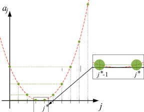
   Figure 4: Representation of $a_{j}$ as a function of $j$ with $j^{\star}$ the location of the minimum of the $\left\{a_{j}\right\}$ for the degenerate case with $2(1+\xi_{B})/\Xi$ an even number.

   The even degeneracy case is represented graphically in fig. 4 where the value of $j^{\star}$ is degenerate and the number of degenerate $a_{j}$’s equates the minimum between $(j^{\star}-1)$ and $(N-j^{\star}+1)$. If $\{j^{{\dagger}}\}$ denotes the set of degenerate values, then the partition function reads from LABEL:eq:laplace_Z_simple,

   $$\mathcal{T}_{\left\{f_{N}\otimes\cdots\otimes f_{0}\right\}}^{\left[\Xi\Delta\right]}(s)= \left[\prod_{k\notin\{j^{\dagger}\}}\frac{1}{s+a_{k}}\right]\left[{\prod_{k\in\{j^{\dagger}\}}}^{\star}\frac{1}{\left(s+a_{k}\right)^{2}}\right]$$ (27)

   $$= \sum_{k\notin\{j^{\dagger}\}}\left\{\prod_{l=0,l\neq k}^{N}\frac{1}{a_{l}-a_{k}}\right\}\frac{1}{s+a_{k}}$$

   $$+{\sum_{k\in\{j^{\dagger}\}}}^{\star}\left\{\prod_{l=0,l\neq k,k^{\dagger}}^{N}\frac{1}{a_{l}-a_{k}}\right\}\left[\frac{1}{\left(s+a_{k}\right)^{2}}-\left(\sum_{l=0,l\neq k,k^{\dagger}}^{N}\frac{1}{a_{l}-a_{k}}\right)\frac{1}{s+a_{k}}\right]$$

   $$= \sum_{k\notin\{j^{\dagger}\}}C_{k}\,\frac{1}{s+a_{k}}+{\sum_{k\in\{j^{\dagger}\}}}^{\star}C_{k,k^{\dagger}}\,\left[\frac{1}{\left(s+a_{k}\right)^{2}}-S_{k,k^{\dagger}}\frac{1}{s+a_{k}}\right],$$

   with $C_{k,k^{\dagger}}=\prod_{l=0,l\neq k,k^{\dagger}}^{N}\frac{1}{a_{l}-a_{k}}$ and $S_{k,k^{\dagger}}=\sum_{l=0,l\neq k,k^{\dagger}}^{N}\frac{1}{a_{l}-a_{k}}$ coefficients simplified to,

   $$C_{k,k^{\dagger}}=-\frac{(-1)^{k+k^{\dagger}}\left(k-k^{\dagger}\right)^{2}}{k!(k^{\dagger})!(N-k)!(N-k^{\dagger})!},$$ (28)

   and

   $$S_{k,k^{\dagger}}=\frac{1}{k-k^{\dagger}} \left\{\frac{2}{k-k^{\dagger}}+\Phi_{0}\left(N-k+1\right)-\Phi_{0}\left(N-k^{\dagger}+1\right)+\Phi_{0}\left(k^{\dagger}+1\right)-\Phi_{0}\left(k+1\right)\right\}.$$ (29)

   Ultimately, the partition function,

   $$\mathcal{Z}= \left(\frac{2\pi\,R^{2}}{\Xi}\right)^{N}\,e^{a_{N}\Xi\Delta-E_{0}}$$ (30)

   $$\times\left(\sum_{k\notin\{j^{\dagger}\}}C_{k}\,e^{-a_{k}\Xi\Delta}+{\sum_{k\in\{j^{\dagger}\}}}^{\star}C_{k,k^{\dagger}}\,\left[\Xi\Delta-S_{k,k^{\dagger}}\right]\,e^{-a_{k}\Xi\Delta}\right).$$

3. The degenerate case: $2(1+\xi_{B})/\Xi$ odd

   

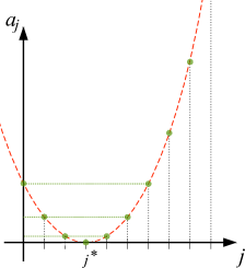
   Figure 5: Representation of $a_{j}$ as a function of $j$ with $j^{\star}$ the location of the minimum of the $\left\{a_{j}\right\}$ for the degenerate case with $2(1+\xi_{B})/\Xi$ an odd number

   Different from the previous case, $j^{\star}$ is not degenerate as shown in fig. 5 and so we would expect that the partition function gives,

   $$\mathcal{Z}= \left(\frac{2\pi\,R^{2}}{\Xi}\right)^{N}\,e^{a_{N}\Xi\Delta-E_{0}}$$ (31)

   $$\times\left(D_{j^{\star}}+\sum_{k\notin\{j^{\dagger}\}\wedge j^{\star}}C_{k}\,e^{-a_{k}\Xi\Delta}+{\sum_{k\in\{j^{\dagger}\}}}^{\star}C_{k,k^{\dagger}}\,\left[\Xi\Delta-S_{k,k^{\dagger}}\right]\,e^{-a_{k}\Xi\Delta}\right),$$

   with

   $$D_{k}=\left(\frac{1}{k!(N-k)!}\right)^{2}.$$ (32)

The partition function is given by three different expressions, (LABEL:eq:exact_Z_non-deg), (LABEL:eq:exact_Z_even-deg) and (LABEL:eq:exact_Z_odd-deg) depending if $4(1+\xi_{B})/\Xi$ is a whole number or not. Since the free energy has to be continuous, the partition function requires the same property. Despite that fact, it is interesting to verify that we can recover (LABEL:eq:exact_Z_even-deg) and (LABEL:eq:exact_Z_odd-deg) from an appropriate limit of (LABEL:eq:exact_Z_non-deg). This is done in appendix A. The rationale proceeding to this argument is to use the non-degenerate partition function from LABEL:eq:exact_Z_non-deg for all future calculations.

III.2 Density profile

The density profile is given by

$$\rho(\mathbf{r})= \frac{N}{N!\,\mathcal{Z}}\int\text{d}^{N}\mathbf{r}\,\delta\left(\mathbf{r}-\mathbf{r}_{1}\right)\,e^{-\mathcal{H}}=\frac{N}{N!\,\mathcal{Z}}\left(\frac{R^{2}}{\Xi}\right)^{N}\int\text{d}^{N}y\text{d}^{N}\theta\,\frac{\delta\left(R\,e^{y/\Xi}-R\,e^{y_{1}/\Xi}\right)}{2\pi\,R\,e^{y/\Xi}}\,e^{-\mathcal{H}+\frac{2}{\Xi}\sum_{j}y_{j}}$$ (33)

$$= \frac{\Xi}{2\pi\,R^{2}\,e^{2y/\Xi}}\left(\frac{2\pi\,R^{2}}{\Xi}\right)^{N}e^{-E_{0}}\frac{N}{N!\,\mathcal{Z}}\int\text{d}^{N}y\,\delta\left(y-y_{1}\right)\,e^{-\mathcal{H}^{\prime}}$$

$$= \frac{\Xi}{2\pi R^{2}e^{2y/\Xi}}\rho_{y}$$

where

$$\rho_{y}\mathrel{\mathop{:}}=N\left\langle\delta\left(y-y_{1}\right)\right\rangle_{\{y_{j}\}}\quad\text{with}\quad\left\langle\delta\left(y-y_{1}\right)\right\rangle_{\{y_{j}\}}\mathrel{\mathop{:}}=\left(\frac{2\pi\,R^{2}}{\Xi}\right)^{N}e^{-E_{0}}\frac{1}{N!\,\mathcal{Z}}\int\text{d}^{N}y\,\delta\left(y-y_{1}\right)\,e^{-\mathcal{H}^{\prime}}$$ (34)

which speaks equally for $\rho$.

The average for $\rho_{y}$ is easily calculated using the procedure for the partition function considering that in the partitioning of the phase space $\left\langle\delta{(y-y_{1})}\right\rangle$ takes $(N-1)!$ permutations with $y_{1}$ at a given position in the group of $\{y_{j}\}$’s. Since each arrangement is obtained through a series of permutations of the [BO] ($y_{1}<y_{2}<\cdots<y_{N}$ denoted by [BO]) then the average yields that

$$N\left\langle\delta\left(y-y_{1}\right)\right\rangle_{\{y_{j}\}}=\left\langle\delta\left(y-y_{1}\right)\right\rangle_{\{y_{j}\}}^{T}+\left\langle\delta\left(y-y_{2}\right)\right\rangle_{\{y_{j}\}}^{T}+\cdots+\left\langle\delta\left(y-y_{N}\right)\right\rangle_{\{y_{j}\}}^{T},$$ (35)

where the $T$ stands for a truncation of the integration to the subregion of the phase space delimited by the [BO] leading to,

$$\left\langle\delta\left(y-y_{k}\right)\right\rangle_{\{y_{j}\}}^{T}= \left(\frac{2\pi\,R^{2}}{\Xi}\right)^{N}\frac{e^{-E_{0}}}{\mathcal{Z}}\int_{\textbf{[BO]}}\text{d}^{N}y\,\delta\left(y-y_{k}\right)e^{-\mathcal{H}^{\prime}}$$ (36)

$$= \left(\frac{2\pi\,R^{2}}{\Xi}\right)^{N}\frac{e^{a_{N}\Xi\Delta-E_{0}}}{\mathcal{Z}}\int_{\textbf{[BO]}}\text{d}^{N}y\,\delta\left(y-y_{k}\right)e^{-\sum_{j=0}^{N}a_{j}(y_{j+1}-y_{j})}.$$

$$= \left(\frac{2\pi\,R^{2}}{\Xi}\right)^{N}\frac{e^{a_{N}\Xi\Delta-E_{0}}}{\mathcal{Z}}\underbrace{\int_{\textbf{[BO]}}\text{d}^{N}y\,\delta\left(y-y_{k}\right)\prod_{j=0}^{N}f_{j}(y_{j+1}-y_{j})}_{\text{recalled as }\delta_{k}^{T}}.$$

The $N!$ steps in to account for all permutations of any given arrangement of the $\{y_{j}\}$’s deriving from the $(N-1)!$ intrinsic permutations times $N$ from the average of the density. Let us evaluate $\delta_{k}^{T}$ term using the Laplace transformation. From the steps followed in eq. 17,

$$\mathcal{T}_{\left\{\delta_{k}^{T}\right\}}^{\left[y\right]}(s) =\int_{0}^{\infty}\text{d}ye^{-s\,y}\left\{\int_{0}^{\Xi\Delta}\text{d}y_{N}\int_{0}^{y_{N}}\text{d}y_{N-1}\dots\int_{0}^{y2}\text{d}y_{1}\,\left(\prod_{j=0}^{N}f_{j}\left(y_{j+1}-y_{j}\right)\right)\delta\left(y-y_{k}\right)\right\}$$

$$=\int_{0}^{\Xi\Delta}\text{d}y_{N}\int_{0}^{y_{N}}\text{d}y_{N-1}\dots\int_{0}^{y2}\text{d}y_{1}\,\left(\prod_{j=0}^{N}f_{j}\left(y_{j+1}-y_{j}\right)\right)\left\{\prod_{l=0}^{k-1}e^{-s(y_{l+1}-y_{l})}\right\}.$$

Defining $g_{j}(x;s)=e^{-s\,x}f_{j}(x)$,

$$\mathcal{T}_{\left\{\delta_{k}^{T}\right\}}^{\left[y\right]}(s) =\left[f_{N}\otimes f_{N-1}\otimes\cdots\otimes f_{k}\otimes g_{k-1}\otimes g_{k-2}\otimes\cdots\otimes g_{1}\otimes g_{0}\right](\Xi\Delta),$$

which again, admits a solution via the Laplace transformation on $\Xi\Delta$; therefore,

$$\mathcal{T}_{\left\{\mathcal{T}_{\left\{\delta_{k}^{T}\right\}}^{\left[y\right]}\right\}}^{\left[\Xi\Delta\right]}(t) =\left(\prod_{j=0}^{k-1}\frac{1}{t+s+a_{j}}\right)\left(\prod_{j=k}^{N}\frac{1}{t+a_{j}}\right)$$

$$=\left(\sum_{j=0}^{k-1}\frac{d_{j,k}(s)}{t+s+a_{j}}+\sum_{j=k}^{N}\frac{d_{j,k}(s)}{t+a_{j}}\right),$$

with

$$d_{j,k}(s)=\begin{cases}\left(\prod_{l=0,l\neq j}^{k-1}\frac{1}{-a_{j}+a_{l}}\right)\left(\prod_{l=k}^{N}\frac{1}{-a_{j}-s+a_{l}}\right),&\mbox{if }j<k\\ \left(\prod_{l=0}^{k-1}\frac{1}{-a_{j}+s+a_{l}}\right)\left(\prod_{l=k,l\neq j}^{N}\frac{1}{-a_{j}+a_{l}}\right),&\mbox{if }j\geq k.\\ \end{cases}$$

The presentation of the previous constants is not convenient for the final inversion. Expanding the second and first products in, respectively, the lower and upper bounds of $j$ we obtain,

$$d_{j,k}(s)= \begin{cases}C_{0,k-1;j}\left(-\sum_{m=k}^{N}C_{k,N;m}\frac{1}{s+a_{j}-a_{m}}\right),&\mbox{if }j<k\\ C_{k,N;j}\left(\sum_{m=0}^{k-1}C_{0,k-1;m}\frac{1}{s-a_{j}+a_{m}}\right),&\mbox{if }j\geq k,\end{cases}$$ (37)

with the constant $C_{m,n;k}=\prod_{l=m,l\neq k}^{n}\frac{1}{a_{l}-a_{k}}$ ($m,n\in\mathcal{N}\mathrel{\ooalign{$\ni$\cr\kern-1.0pt$-$\kern-6.5pt$-$}}m<n\,\wedge\,k\in[m,n]$), evaluated equally as $C_{k}$ in eq. 24, given by,

$$C_{m,n;k}=\frac{2(-1)^{k-m}}{(k-m)!\left(n-k\right)!}\frac{\left(k-\left[\frac{\xi-1}{\Xi}+\frac{1}{2}\right]\right)\,\mathbf{\Gamma}\left(m+k-2\left[\frac{\xi-1}{\Xi}+\frac{1}{2}\right]\right)}{\mathbf{\Gamma}\left(n+1+k-2\left[\frac{\xi-1}{\Xi}+\frac{1}{2}\right]\right)}$$ (38)

The first inversion yields,

$$\mathcal{T}_{\left\{\delta_{k}^{T}\right\}}^{\left[y\right]}(s)= \sum_{j=0}^{k-1}d_{j,k;s}\,e^{-(s+a_{j})\Xi\Delta}+\sum_{j=k}^{N}d_{j,k;s}\,e^{-a_{j}\Xi\Delta}$$

$$= -\sum_{j=0}^{k-1}\sum_{m=k}^{N}C_{0,k-1;j}\,C_{k,N;m}\,\frac{e^{-(s+a_{j})\Xi\Delta}}{s+a_{j}-a_{m}}+\sum_{j=k}^{N}\sum_{m=0}^{k-1}C_{k,N;j}\,C_{0,k-1;m}\,\frac{e^{-a_{j}\Xi\Delta}}{s-a_{j}+a_{m}},$$

which is invertible noticing that the first term is proportional to $\Theta(y-\Xi\Delta)$, the Heaviside step function, hence trivial since $y\leq\Xi\Delta$. Finally, the truncated density reads,

$$\left\langle\delta\left(y-y_{k}\right)\right\rangle_{\{y_{j}\}}^{T}= \frac{\sum_{j=k}^{N}\sum_{l=0}^{k-1}C_{k,N;j}\,C_{0,k-1;l}\,e^{-a_{j}\Xi\Delta-(a_{l}-a_{j})y}}{\sum_{j=0}^{N}C_{j}\,e^{-a_{j}\Xi\Delta}}$$ (39)

$$= \frac{\left\{\sum_{j=k}^{N}C_{k,N;j}\,e^{-a_{j}(\Xi\Delta-y)}\right\}\left\{\sum_{j=0}^{k-1}C_{0,k-1;j}\,e^{-a_{j}y}\right\}}{\sum_{j=0}^{N}C_{j}\,e^{-a_{j}\Xi\Delta}}$$

The previous formulation for the density teaches us many things about the behavior of the density close to $R$ and $D$. First of all, inspecting the above relationship we find that,

$$\left\langle\delta\left(y-y_{k}\right)\right\rangle_{\{y_{j}\}}^{T}\propto \frac{\mathcal{Z}[\Xi,\xi,k-1,\Delta-y/\Xi]\,\times\,\mathcal{Z}[\Xi,\xi,N-k,y/\Xi]}{\mathcal{Z}[\Xi,\xi,N,\Delta]},$$ (40)

the truncated profile at a given position equates the product of partition functions corresponding to $k-1$ particles before that position and $N-k$ particles beyond the latter. This trait is characteristic of decorrelated fluids as presumed in the mean field regime.

Summarizing, if we define $\widetilde{\rho}(\mathbf{r})=2\pi\,R^{2}\rho(\mathbf{r})/(N\xi)$, the density profile is given by

$$\widetilde{\rho}(\mathbf{r})=\frac{\Xi}{N\xi}\left(\frac{R}{r}\right)^{2}\sum_{k=1}^{N}\frac{\left\{\sum_{j=k}^{N}C_{k,N;j}\,\left(\frac{D}{r}\right)^{-a_{j}\Xi}\right\}\left\{\sum_{j=0}^{k-1}C_{0,k-1;j}\,\left(\frac{r}{R}\right)^{-a_{j}\Xi}\right\}}{\sum_{j=0}^{N}C_{j}\,\left(\frac{D}{R}\right)^{-a_{j}\Xi}}.$$ (41)

From the previous relationship we can extract the leading behavior of the weakly coupled regime which turns out to be precisely that of mean field; $\rho\propto 1-2x/\mu$ with $x$ the perpendicular distance from the disk and $\mu$ the Gouy length.

On the other hand, as $\Xi\Delta$ becomes large, the functional form of the profile simplifies close to both boundaries. Knowing that the first term (that which sums from $k$ to $N$) will be non–zero, or, the least, relevant, if $k\leq j^{\star}$ comparing to the partition function which scales as $e^{-a_{j^{\star}}\Xi\Delta}$ from LABEL:eq:approx_Z_non-deg. Conversely, for the outer shell, or close to $D$, the situation is that which the second term is non–zero if $k>j^{\star}$. This provides an interesting parallel rationale to condensation. Those particles which contribute to the profile near the surface, i.e. the condensed population, are $j^{\star}$. On the other hand, the remaining $N-j^{\star}$ contribute to the profile at the outer shell. Approximating from LABEL:eq:exact_rho_T and looking at the profile near $R$ we are examining the truncated profiles for the case of $k\leq j^{\star}$ since all profiles of index beyond $j^{\star}$ will correspond to evaporated counter-ions. Hence,

$$\left\langle\delta\left(y-y_{k}\right)\right\rangle_{\{y_{j}\}}^{T}\simeq \sum_{j=0}^{k-1}\frac{C_{0,k-1;j}}{C_{0,k-1;j^{\star}}}\,e^{-(a_{j}-a_{j^{\star}})y}$$ (42)

$$+\left[\sum_{j=0}^{k-1}\frac{C_{0,k-1;j}C_{k,N;j^{\star}\pm 1}}{C_{0,N;j^{\star}}}\,e^{-(a_{j}-a_{j^{\star}\pm 1})y}-\frac{C_{j^{\star}\pm 1}}{C_{j^{\star}}}\sum_{j=0}^{k-1}\frac{C_{0,k-1;j}}{C_{0,k-1;j^{\star}}}\,e^{-(a_{j}-a_{j^{\star}})y}\right]\,e^{-(a_{j^{\star}\pm 1}-a_{j^{\star}})\Xi\Delta}$$

$$+\mathcal{O}\left(e^{-2\Xi\Delta}\right).$$

Conversely the contribution to the exterior shell reads for $k>j^{\star}$,

$$\left\langle\delta\left(y-y_{k}\right)\right\rangle_{\{y_{j}\}}^{T}\simeq \sum_{j=k}^{N}\frac{C_{k,N;j}}{C_{k,N;j^{\star}}}e^{-(a_{j}-a_{j^{\star}})(\Xi\Delta-y)}$$ (43)

$$+\left[\sum_{j=k}^{N}\frac{C_{0,k-1;j^{\star}\pm 1}C_{k,N;j}}{C_{0,N;j^{\star}}}e^{-(a_{j}-a_{j^{\star}\pm 1})(\Xi\Delta-y)}-\frac{C_{j^{\star}\pm 1}}{C_{j^{\star}}}\sum_{j=k}^{N}\frac{C_{k,N;j}}{C_{k,N;j^{\star}}}e^{-(a_{j}-a_{j^{\star}})(\Xi\Delta-y)}\right]\,e^{-(a_{j^{\star}\pm 1}-a_{j^{\star}})\Xi\Delta}$$

$$+\mathcal{O}\left(e^{-y-\Xi\Delta}\right),$$

sharing the same functional form at both edges. Notice that the density, according to the procedure we have followed, is written as an expansion of powers of the radial distance.

\psfrag{AX}{$r/R$}\psfrag{BY}{$\widetilde{\rho}$}\includegraphics[width=216.81pt]{fig6}

Figure 6: The density profile $\widetilde{\rho}$ near the charged disk for different values of the Manning parameter for $N=10$. The data displays the results for different box sizes. The dashed curves represent the analytic prediction LABEL:eq:exact_rho_T into eq. 33. The values for the Manning parameter are chosen for small $\Xi$ and very close to unity where the theory is no longer valid.

Now we turn to fig. 6 where the comparison between the analytic prediction and the simulation results is displayed. From the results, the deviations from the data, as expected, increase with higher coupling (see $\xi=9$ in the plot). Notice that despite the differences the contact density as the profile approaches to $r=R$ matches that reached by the analytic profile.

III.3 Integrated charge

The integrated charge amounts to the number of condensed counter-ions from the density profile LABEL:eq:exact_rho_T. The integrated charge reads in terms of the centrifugal variables $\{y_{j}=\Xi\log({r}_{j}/{R})\}$ as follows,

$$Q(r)= \int_{0}^{y}{\rho_{y}}({y^{\prime}})\,\text{d}{y^{\prime}}=\sum_{k=1}^{N}Q_{k}(y),$$ (44)

that split into contributions of each truncated density reads,

$$Q_{k}(r)= \frac{\sum_{j=k}^{N}\left\{C_{k,N;j}\,e^{-a_{j}\Xi\Delta}\left[\sum_{l=0}^{k-1}\frac{C_{0,k-1;l}}{a_{l}-a_{j}}\,\left(1-e^{-(a_{l}-a_{j})y}\right)\right]\right\}}{\sum_{j=0}^{N}C_{j}\,e^{-a_{j}\Xi\Delta}},$$ (45)

with particular emphasis on a functional form suited for distances close to $R$, or,

$$Q_{k}(r)= 1-\frac{\sum_{j=0}^{k-1}\left\{e^{-a_{j}\Xi\Delta}\left[C_{j}-C_{0,k-1;j}\sum_{l=k}^{N}\frac{e^{-(a_{l}-a-j)(\Xi\Delta-y)}C_{k,N;l}}{a_{l}-a_{j}}\right]\right\}}{\sum_{j=0}^{N}C_{j}\,e^{-a_{j}\Xi\Delta}},$$ (46)

corresponding to that closest to $D$. Notices how the two functional forms consistently show that when $y\to 0$ (close to $R$) $Q_{k}\to 0$ and $y\to\Xi\Delta$ (close to $D$) $Q_{k}\to 1$ as expected since the truncated densities corresponds to the contribution of a single particle in the [BO].

In order to understand how many ions condense, let us look at eq. 45 and notice that when $\Delta$ is large compared to $y$, $Q_{k}\to 0$ if $k>j^{\star}$ and so the condensed counter-ions will equate $j^{\star}$, an argument consistent with what we have assumed constructing the density profile for infinite box sizes. With regards to condensation, it means that the fraction of condensed ions is $f=\frac{j^{\star}}{N}$, with special attention to a minor, yet relevant, detail of the density profile. For simplicity we have omitted the degeneracy issue here considering that the pressure is a continuous function. Therefore, the density profiles should not exhibit any particular behavior at the troublesome values. As a matter of fact, there is one problem when $a_{j^{\star}}=a_{j^{\star}-1}$, as discussed earlier, where the profile behaves as $\rho\sim 1/r^{2}$ and the corresponding integrated quantity $Q_{j^{\star}}(r)\simeq y/(\Xi\Delta)$. This form tells us that the condensing counter-ion is evenly distributed in the box (using $y$ coordinates). An important rationale then for condensation is that this particle is neither condensed nor evaporated and, thus, the integrated charge will exhibit a constant slope form when this occurs. This situation does not take place in the three-dimensional case (Naji and Netz, 2005, 2006; Mallarino et al., 2013).

With this matter clarified, the fraction of condensed counter-ions corresponds then to,

$${\color[rgb]{0.0,0.0,0.0}f=\frac{1}{N}\left\lceil\frac{\xi-1}{\Xi}\right\rceil=\frac{1}{N}\left\lceil\frac{f_{M}N}{1+\frac{\xi_{B}}{\xi}}\right\rceil}.$$ (47)

\psfrag{AX}{$r/R$}\psfrag{BY}{$\widetilde{\rho}$}\psfrag{AX}{$\log(r/R)$}\psfrag{BY}{$N-Q(r)$}\includegraphics[width=216.81pt]{fig7}

Figure 7: The integrated charge $N-Q({r})$ as a function of the logarithmic distance for $\Delta=10^{2}$, $\xi_{B}=0$ and $N=10$ for various $\Xi$. The plots read for the coupling parameter from top to bottom $\Xi=\frac{2}{5},\frac{10}{21},\frac{1}{2},\frac{10}{19},\frac{2}{3},\frac{10}{11},1,\frac{10}{9}$ and $2$.

The numerical results from Monte Carlo simulations are presented in fig. 7 highlighting the evaporated counter-ions as indicated by the plateau. We observe that, at the transitions, the integrated charge displays a constant slope form associated to the counter-ion which lies at the borderline of condensation (in fig. 7, $\Xi=1/2,\,1$). Away from the transitions the plateau is flat similar to the three dimensional case.

The onset for condensation in two dimensions coincides with the well-known result $\xi=1$. This signals a transition between the regime of full evaporated to partially condensed counter-ions. However, the details of the behavior beyond this point are unique to the two dimensional problem. Unlike the situation in three dimensions, the thermodynamic limit ($N\to\infty$), at a fixed Manning parameter and no charge in the exterior boundary ($\xi_{B}=0$), takes the coupling to zero, which is the mean field regime investigated thoroughly in previous works. In such a case, $f\to f_{M}=1-\frac{1}{\xi}$.

The situation maintaining a fixed, non vanishing, coupling constant $\Xi$ and $N\to\infty$ will imply an infinite Manning parameter $\xi\to\infty$, and consequently a strongly bound set of counter-ions. However, despite the situation, the number of condensed counter-ions increases with $N$ while the remaining evaporated remains all the same. This is easy to see from eq. 20 where the number of evaporated ione is,

$$N_{\text{evap}}=\left\lfloor\frac{1+\xi_{B}}{\Xi}\right\rfloor.$$ (48)

In other words, evaporation, looking at $\xi>1$ is dominated by the coupling parameter. This is the reason for the division of the two dimensional case between $\Xi<1$, $\Xi=1$, and $\Xi>1$; assuming that $\xi_{B}=0$ if $\Xi<1$ there is evaporation, $\Xi>1$ full condensation, leaving $\Xi=1$ the critical value for the coupling parameter where there is only one unbound counter-ion. From the earlier considerations, the problem with $\Xi=1$ will have, exactly, one free ion while the problem for greater couplings is equivalent to full condensation. This ultimate remark helps to find an analytic route towards the profile for large couplings and the contact theorem.

One question that rises with the previous result is what is the effective charge of the center disk and the ion cloud. For simplicity we assume that $Q_{1}>0$. The condensed ions will screen the charge of the center disk thus reducing the mean potential interaction between the center region and the ions in the outer region of the disk. In other words, what is the value of $\xi_{\text{eff}}\mathrel{\mathop{:}}=\xi-N_{c}\Xi$?

$$\xi_{\text{eff}}=\Xi\left\lfloor\frac{1+\xi_{B}}{\Xi}\right\rfloor-\xi_{B},$$ (49)

which tells us that $\xi_{\text{eff}}\leq 1$ for any coupling and exterior charge $Q_{2}$; also, if $\Xi\leq 1$ then $\xi_{\text{eff}}\geq 0$; lastly, if $\xi_{B}=0$ then $\xi_{\text{eff}}\geq 0$. However, if $\Xi>1$ the effective charge could be negative only if $Q_{2}\neq 0$! This striking effect, similar to charge inversion, is only possible at strong couplings.

III.4 Contact density

For the contact density, we turn to LABEL:eq:exact_rho_T at $y=0$ and $y=\Delta$. In both cases, we encounter that the truncated densities have vanishing values except for two particular cases. For $y=0$,

$$\left.\left\langle\delta\left(y-y_{k}\right)\right\rangle_{\{y_{j}\}}^{T}\right|_{y=0}=\left\{\begin{array}[]{cc}\frac{\sum_{j=1}^{N}C_{1,N;j}\,e^{-a_{j}\Xi\Delta}}{\sum_{j=0}^{N}C_{j}\,e^{-a_{j}\Xi\Delta}}&k=1\\ 0&k>0\end{array}\right.,\\$$ (50)

likewise for $y=\Xi\Delta$,

$$\left.\left\langle\delta\left(y-y_{k}\right)\right\rangle_{\{y_{j}\}}^{T}\right|_{y=\Xi\Delta}=\left\{\begin{array}[]{cc}0&k<N\\ \frac{\sum_{j=0}^{N-1}C_{0,N-1;j}\,e^{-a_{j}\Xi\Delta}}{\sum_{j=0}^{N}C_{j}\,e^{-a_{j}\Xi\Delta}}&k=N\end{array}\right.,\\$$ (51)

because

$$\sum_{j=l}^{m}C_{l,m;j}=\sum_{j=l}^{m}\left[\prod_{k=l,k\neq j}^{m}\frac{1}{a_{k}-a_{j}}\right]=\delta_{l,m}$$

that tells us which terms contribute to the contact densities. Although, this is not surprising since the arrangement of the [BO] intuitively truncates the average to contributions to both contacts coming from the first and last particles.

Taking the large box limit, eqs. 50 and 51 yield,

$$\widetilde{\rho}(R)=\frac{1}{N\,\xi}(a_{0}-a_{j^{\star}})=\left(f_{M}-\left[f_{M}-\frac{j^{\star}}{N}\right]\right)\left(f_{M}+\left[f_{M}-\frac{j^{\star}}{N}\right]+\frac{1}{N}\right),$$ (52)

and,

$$e^{2\Delta}\widetilde{\rho}(D)=\frac{1}{N\,\xi}(a_{N}-a_{j^{\star}})=\left(\frac{1}{\xi}-\left[f_{M}-\frac{j^{\star}}{N}\right]-\frac{1}{N}\right)\left(\frac{1}{\xi}+\left[f_{M}-\frac{j^{\star}}{N}\right]\right),$$ (53)

recovering mean field’s result by taking $N\to\infty$ where $\widetilde{\rho}(R)=f_{M}^{2}$ and $e^{2\Delta}\widetilde{\rho}(D)=(1-f_{M})^{2}$. Additionally, note that the value of the density at contact ($r=R$) is non-zero for $\xi>1$ coinciding with the onset for condensation discussed earlier. As expected when all ions condense, or $j^{\star}/N\to 1$, the density at the exterior shell vanishes.

\psfrag{AX}{$r/R$}\psfrag{BY}{$\widetilde{\rho}$}\psfrag{AX}{$\log(r/R)$}\psfrag{BY}{$N-Q(r)$}\psfrag{AX}{$\Xi$}\psfrag{BY}{$\widetilde{\rho}|_{r=R}$}\psfrag{BY2}{$\xi^{2}e^{2\Delta}\widetilde{\rho}|_{r=D}$}\includegraphics[width=164.77771pt]{fig8a.eps}

(a)

\psfrag{AX}{$r/R$}\psfrag{BY}{$\widetilde{\rho}$}\psfrag{AX}{$\log(r/R)$}\psfrag{BY}{$N-Q(r)$}\psfrag{AX}{$\Xi$}\psfrag{BY}{$\widetilde{\rho}|_{r=R}$}\psfrag{BY2}{$\xi^{2}e^{2\Delta}\widetilde{\rho}|_{r=D}$}\includegraphics[width=164.77771pt]{fig8b.eps}

(b)

Figure 8: The density $\widetilde{\rho}$ at contact in $r=R$ as a function of the Coupling parameter $\Xi$ with $\xi_{B}=0$; here, $\Delta$ varies and $N=10$. The range of $\Xi$ extends below the onset for condensation up to high couplings. The dashed curves represent the exact contact density taken from evaluating the density from eq. 33. We considered the analytic exact result since $\Delta$ is small. The arrows indicate the location of $\Xi=1$, the borderline to strong coupling.

\psfrag{AX}{$r/R$}\psfrag{BY}{$\widetilde{\rho}$}\psfrag{AX}{$\log(r/R)$}\psfrag{BY}{$N-Q(r)$}\psfrag{AX}{$\Xi$}\psfrag{BY}{$\widetilde{\rho}|_{r=R}$}\psfrag{BY2}{$\xi^{2}e^{2\Delta}\widetilde{\rho}|_{r=D}$}\psfrag{AX}{$\Xi$}\psfrag{BY}{$\widetilde{\rho}|_{r=R}$}\psfrag{BY2}{$\xi^{2}e^{2\Delta}\widetilde{\rho}|_{r=D}$}\includegraphics[width=164.77771pt]{fig9a.eps}

(a)

\psfrag{AX}{$r/R$}\psfrag{BY}{$\widetilde{\rho}$}\psfrag{AX}{$\log(r/R)$}\psfrag{BY}{$N-Q(r)$}\psfrag{AX}{$\Xi$}\psfrag{BY}{$\widetilde{\rho}|_{r=R}$}\psfrag{BY2}{$\xi^{2}e^{2\Delta}\widetilde{\rho}|_{r=D}$}\psfrag{AX}{$\Xi$}\psfrag{BY}{$\widetilde{\rho}|_{r=R}$}\psfrag{BY2}{$\xi^{2}e^{2\Delta}\widetilde{\rho}|_{r=D}$}\includegraphics[width=164.77771pt]{fig9b.eps}

(b)

Figure 9: The density $\widetilde{\rho}$ at contact in $r=R$ as a function of the Coupling parameter $\Xi$ with $\xi_{B}=0$; here, $\Delta$ varies and $N=10$. The range of $\Xi$ extends below the onset for condensation up to high couplings. The dashed curves represent the exact contact density taken from evaluating the density from eq. 33. We considered the analytic exact result since $\Delta$ is small. The arrows indicate the location of $\Xi=1$, the borderline to strong coupling.

The values compare very well with the simulation data from figs. 8a and 8b considering a small $\Delta$. Notice that the contact densities are continuous functions; for $r=R$ the function does not present any appreciable or qualitative changes while its exterior counterpart shows a succession of bumps coming from the evaporated counter-ions. Seen that increasing $\Delta$ bolsters the transitions we plot the contacts at $\Delta=10^{2}$ in fig. 10.

\psfrag{AX}{$r/R$}\psfrag{BY}{$\widetilde{\rho}$}\psfrag{AX}{$\log(r/R)$}\psfrag{BY}{$N-Q(r)$}\psfrag{AX}{$\Xi$}\psfrag{BY}{$\widetilde{\rho}|_{r=R}$}\psfrag{BY2}{$\xi^{2}e^{2\Delta}\widetilde{\rho}|_{r=D}$}\psfrag{AX}{$\Xi$}\psfrag{BY}{$\widetilde{\rho}|_{r=R}$}\psfrag{BY2}{$\xi^{2}e^{2\Delta}\widetilde{\rho}|_{r=D}$}\psfrag{AX}{$\Xi$}\psfrag{BY}{{\color[rgb]{0,0.6,0} $\widetilde{\rho}|_{r=R}$}}\psfrag{BY2}{{\color[rgb]{1.0,0.0,0.0} $\xi^{2}e^{2\Delta}\widetilde{\rho}|_{r=D}$}}\includegraphics[width=164.77771pt]{fig10}

Figure 10: The density $\widetilde{\rho}$ at contact in $r=R$ (red) and $r=D$ (olive green) as a function of the Manning parameter; here, $\Delta=100$ and $N=10$. The range of $\xi$ extends below the onset for condensation up to high couplings. The dashed curves represent the $\Delta\to\infty$ formulation from eqs. 52 and LABEL:eq:contact_rho_D_DeltaLimit. The arrows indicate the location of $\Xi=1$, the borderline to strong coupling.

The prediction gives a very accurate estimate of the contact densities seen in the figures at all ranges. Observe that the data displayed considers values of the Manning parameter which fall out of the scope of the present course; at $\Xi=1$ ($\Gamma=2$) we have the drastic change of behavior to strong coupling, as indicated in figs. 8, 9 and 10.

III.5 Energy

The energy for the system can be found with the derivative of the partition function from LABEL:eq:approx_Z_non-deg with respect to $\xi$. Then,

$$\widetilde{E}= -\frac{\xi}{N}\frac{\partial{\left(\log\mathcal{Z}\right)}}{\partial{\xi}},$$

which simplifies in the large $\Delta$ limit to,

$$\widetilde{E}\simeq\xi\Delta\left(\frac{N+1-j^{\star}}{N}\right)\left(\frac{N-j^{\star}}{N}\right).$$ (54)

This equation for the energy has a saw-like shape, as was acknowledged by Naji and Netz (2006, 2005) and explored via the aforementioned procedure for $\Xi<1$ by Burak and Orland (2006), due to the transitions at temperatures below the critical temperature ($\xi>1$) when $N/\xi$ becomes a whole number. Figure 11 presents the numerical results for two values of $\Delta$ displaying, as anticipated, the effect of the box size to the transitions. Notice that for $\Xi>1$ ($\Gamma>2$) the energy goes below zero due to the interaction among the counter-ions.

\psfrag{AX}{$r/R$}\psfrag{BY}{$\widetilde{\rho}$}\psfrag{AX}{$\log(r/R)$}\psfrag{BY}{$N-Q(r)$}\psfrag{AX}{$\Xi$}\psfrag{BY}{$\widetilde{\rho}|_{r=R}$}\psfrag{BY2}{$\xi^{2}e^{2\Delta}\widetilde{\rho}|_{r=D}$}\psfrag{AX}{$\Xi$}\psfrag{BY}{$\widetilde{\rho}|_{r=R}$}\psfrag{BY2}{$\xi^{2}e^{2\Delta}\widetilde{\rho}|_{r=D}$}\psfrag{AX}{$\Xi$}\psfrag{BY}{{\color[rgb]{0,0.6,0} $\widetilde{\rho}|_{r=R}$}}\psfrag{BY2}{{\color[rgb]{1.0,0.0,0.0} $\xi^{2}e^{2\Delta}\widetilde{\rho}|_{r=D}$}}\psfrag{AX}{$\xi$}\psfrag{BY}{$\widetilde{E}/\Delta$}\includegraphics[width=164.77771pt]{fig11}

Figure 11: The energy as a function of the Manning parameter; here $N=10$ and $\Delta=20,10^{2}$. The dashed curve corresponds to the $\Delta\to\infty$ prediction from eq. 54.

Related to the problem of condensation and minimal free energy, the energy shift at any transition is given for the change of energy when an unbound ion is condensed. Then,

$$\mu_{evap}^{(2D)}= N\left[\xi_{j^{\star}}\Delta\left(\frac{N+1-j^{\star}}{N}\right)\left(\frac{N-j^{\star}}{N}\right)-\xi\Delta\left(\frac{N+1-j^{\star}-1}{N}\right)\left(\frac{N-j^{\star}-1}{N}\right)\right]$$ (55)

$$= 2\Delta,$$

which, unsurprisingly, coincides with the entropy cost for binding a free ion, a discussion thoroughly stripped by Manning (1969b).

IV The $\Xi=1$ case

The case when $\Xi=1$, or $\Gamma=2$, represents the borderline before full condensation and also could be understood as the limiting situation before the strong coupling regime. This situation admits an exact formulation that is interesting to explore. To begin with, let us look at the Boltzmann factor of the Hamiltonian eq. 5 as it reads,

$$e^{-\mathcal{H}}= e^{-E_{0}}\prod_{j=1}^{N}\left|\frac{\mathbf{r}_{j}}{R}\right|^{-2\xi}\,\,\prod_{1\leq j<k\leq N}\left|\frac{\mathbf{r}_{j}-\mathbf{r}_{k}}{R}\right|^{2\Xi}\,.$$ (56)

For this Hamiltonian, it is always convenient to refer vectors into a complex number in order to simplify the evaluation of the partition function, and from it the correlation functions. That way, we will define

$$z_{j}\mathrel{\mathop{:}}= \frac{r_{j}}{R}\,e^{i\theta_{j}}.$$ (57)

The partition function of the system (eq. 56) is rewritten as,

$$\mathcal{Z}= \frac{R^{2N}e^{-E_{0}}}{N!}\int\left[\prod_{1\leq j<k\leq N}\left|z_{j}-z_{k}\right|^{2}\right]^{\Xi}\prod_{j=1}^{N}|z_{j}|^{-2\xi+1}\text{d}{|z_{j}|}\text{d}{\theta_{j}}$$ (58)

Appealing to the value of the coupling, it is clear from the previous form that $\Xi=1$ simplifies the calculation. Indeed, the procedure to solve the previous integration has been widely used to solve two dimensional systems for $\Gamma=2$ (see Deutsch et al., 1979; Jancovici, 1981) and for $\Gamma=2n$ described by Šamaj et al. (1994) and Téllez and Forrester (1999).

Holding $\Xi=1$ the calculation concerns the Vandermonde determinant in complex variables. Here,

$$\mathsf{V}_{N\times N}= \prod_{1\leq j<k\leq N}(z_{j}-z_{k})$$ (59)

$$= \text{Det}\left[\begin{array}[]{ccccc}1&1&1&\dots&1\\ z_{1}&z_{2}&z_{3}&\dots&z_{N}\\ z_{1}^{2}&z_{2}^{2}&z_{3}^{2}&\dots&z_{N}^{2}\\ .&.&.&\dots&.\\ .&.&.&\dots&.\\ .&.&.&\dots&.\\ z_{1}^{N-1}&z_{2}^{N-1}&z_{3}^{N-1}&\dots&z_{N}^{N-1}\\ \end{array}\right]$$

$$= \sum_{P}\sigma({P})\prod_{j=1}^{N}z_{j}^{P(j)}=\sum_{P}\sigma({P})\prod_{j=1}^{N}|z_{j}|^{P(j)}e^{iP(j)\theta_{j}},$$

where $P$ and $P^{\prime}$ are permutations of $\{0,1,2,...,N-1\}$, and $\sigma(P)$ the respective permutation signature ($\sigma(P)=\pm 1$). Directly to the partition function,

$$\mathcal{Z}= \frac{R^{2N}e^{-E_{0}}}{N!}\sum_{P,P^{\prime}}\sigma({P})\sigma({P^{\prime}})\prod_{j=1}^{N}\underbrace{\int_{0}^{2\pi}\text{d}{\theta_{j}}e^{i(P(j)-P^{\prime}(j))\theta_{j}}}_{{2\pi\delta_{P(j),P^{\prime}(j)}}}\int_{e^{-\Delta}}^{1}|z_{j}|^{P(j)+P^{\prime}(j)-2(\xi-1)-1}\text{d}|z_{j}|,$$ (60)

which defining $\gamma(\Delta,\xi,j)$

$$\gamma(\Delta,\xi,j)= 2\int_{1}^{e^{\Delta}}t^{2(j-(\xi-1))-1}\text{d}t$$ (61)

$$= \left\{\begin{array}[]{lr}2\Delta&\text{for }j=\xi-1\\ \frac{1-e^{2(j-(\xi-1))\Delta}}{(\xi-1)-j}&\text{for }j\neq\xi-1\\ \end{array}\right.,$$

reads,

$$\mathcal{Z}= (\pi R^{2})^{N}e^{-E_{0}}\prod_{j=1}^{N}\gamma(\Delta,\xi,j-1)\underbrace{\left[\frac{1}{N!}\sum_{P,P^{\prime}}\sigma({P})\sigma({P^{\prime}})\delta_{P,P^{\prime}}\right]}_{\color[rgb]{0.0,0.0,1.0}1}.$$

Finally, simplifying yields,

$$\mathcal{Z}= (\pi R^{2})^{N}e^{-E_{0}}\prod_{j=1}^{N}\gamma(\Delta,\xi,j-1).$$ (62)

IV.0.1 Large $\Delta$ limit

The large box size is characterized by the effect of $\Delta$ in the solutions. We can observe that to the present case it enters directly in $\gamma$ in such a way that if $\Delta\to\infty$,

$$\gamma(\Delta,\xi,j)\simeq \left\{\begin{array}[]{lr}2\Delta&\text{for }j=\xi-1\\ \frac{1}{(\xi-1)-j}&\text{for }j<\xi-1\\ \frac{e^{2(j-(\xi-1))\Delta}}{j-(\xi-1)}&\text{for }j>\xi-1\\ \end{array}\right..$$ (63)

This teaches us that only those values of $j<\xi-1$ are independent of the box size and consequently are responsible for the condensed counter-ions. Countrarywise, the remaining entail the behavior of the evaporated population. A priori, by inspection of eq. 62, the total condensed counter-ions are $\left\lfloor\xi\right\rfloor-1$; ergo, for the particular $\xi_{B}=0$ case, neutrality imposes $\xi=N$, which dictates that $N-1$ particles condense and only one particle is unbound, consistent with the results obtained in the previous section for $\Xi<1$.

On the other hand, the evaporated counterpart has two different solutions: one proportional to $\Delta$ and that which grows exponentially with the box size. Related to the problem of condensation, we acknowledged full condensation beyond $\Xi=1$ ($\Gamma=2$) which tells us that this solution stands at the borderline. Then, according to the analysis on the profile the functional form that best suites this situation is that where the density decays like $r^{-2}$.

IV.1 Density profile

The $n$-body distribution functions can be obtained by a procedure used in random matrix theory Mehta (2004) for the circular unitary ensemble. To this end, let us introduce the kernel

$$K(z_{j},z_{k})=\sum_{l=1}^{N}\frac{|z_{j}z_{k}|^{l-1-\xi}e^{i(l-1)(\theta_{k}-\theta_{j})}}{\gamma(\Delta,\xi,l-1)},$$ (64)

Then, following Mehta (2004) (Chap. 5 and 10), it follows that

$$\rho(\mathbf{r})=\frac{1}{\pi R^{2}}K(z,z)$$ (65)

and finally,

$$\rho(\mathbf{r})=\frac{1}{\pi R^{2}}\left[\frac{R}{r}\right]^{2}\sum_{l=1}^{N}\frac{\left(\frac{r}{R}\right)^{2(l-\xi)}}{\gamma(\Delta,\xi,l-1)},$$ (66)

where, for $\widetilde{\rho}=2\pi\,R^{2}\rho/(N\xi)$, this yields,

$$\widetilde{\rho}(r)=\frac{2}{N\xi}\left[\frac{R}{r}\right]^{2}\sum_{l=1}^{N}\frac{\left(\frac{r}{R}\right)^{2(l-\xi)}}{\gamma(\Delta,\xi,l-1)}.$$ (67)

The profile is presented in fig. 12 comparing to the results from Monte Carlo simulations with excellent agreement with the above exact result. Notice the profile exhibits a sequence of terms with power shape. This resembles the situation obtained for $\Xi<1$ ($\Gamma<2$) referred in section III.2.

Particularly for $\xi_{B}=0$ the Manning parameter equates the number of ions, then,

$$\widetilde{\rho}(r) =\frac{2}{N^{2}}\left[\frac{R}{r}\right]^{2}\left\{\sum_{m=1}^{N-1}\frac{1}{\gamma(\Delta,N,N-m-1)}\left(\frac{R}{r}\right)^{2m}+\frac{1}{N\xi\,\Delta}\right\}$$ (68)

$${\color[rgb]{0.0,0.0,0.0}\,\overset{\Delta\to\infty}{=}\,\frac{2}{N^{2}}\left[\frac{R}{r}\right]^{2}\left\{\frac{1}{N\xi\,\Delta}+\left(\frac{R}{r}\right)^{2}\frac{1-N\left(\frac{R}{r}\right)^{2(N-1)}+(N-1)\left(\frac{R}{r}\right)^{2N}}{\left(1-\left(\frac{R}{r}\right)^{2}\right)^{2}}\right\}}$$

Earlier in the situation for weak couplings for $\Xi=1$ we have $j^{\star}=N$; then, it determines that $a_{m}-a_{j^{\star}}=(N-m)(N-m-1)$ a quantity that is always a whole number and particularly for $m=N-1$ is zero. This tells us that the contribution to $\rho$ of one of the summands comes as $r^{-2}$ (see LABEL:eq:exact_rho_T). Additionally, the density from eq. 42 is written in terms of a sum of powers of the ratio between the radial distance and the radius of the cylinder, a result that holds at $\Xi=1$ ($\Gamma=2$). Although the two problems match qualitatively, a quantitative comparison demonstrates the limitations of the procedure followed for weak couplings in section III, the angular uncorrelated fluid limit.

\psfrag{AX}{$r/R$}\psfrag{BY}{$\widetilde{\rho}$}\psfrag{AX}{$\log(r/R)$}\psfrag{BY}{$N-Q(r)$}\psfrag{AX}{$\Xi$}\psfrag{BY}{$\widetilde{\rho}|_{r=R}$}\psfrag{BY2}{$\xi^{2}e^{2\Delta}\widetilde{\rho}|_{r=D}$}\psfrag{AX}{$\Xi$}\psfrag{BY}{$\widetilde{\rho}|_{r=R}$}\psfrag{BY2}{$\xi^{2}e^{2\Delta}\widetilde{\rho}|_{r=D}$}\psfrag{AX}{$\Xi$}\psfrag{BY}{{\color[rgb]{0,0.6,0} $\widetilde{\rho}|_{r=R}$}}\psfrag{BY2}{{\color[rgb]{1.0,0.0,0.0} $\xi^{2}e^{2\Delta}\widetilde{\rho}|_{r=D}$}}\psfrag{AX}{$\xi$}\psfrag{BY}{$\widetilde{E}/\Delta$}\psfrag{AX}{$r/R$}\psfrag{BY}{$\widetilde{\rho}$}\includegraphics[width=164.77771pt]{fig12}

Figure 12: The density profile $\widetilde{\rho}$ near the charged disk for different values of the Manning parameter for $N=\xi$; here $\Delta=20$. The dashed curves represent the exact profile from eq. 67. The axis are in logarithmic to show the trend at short and long distances.

IV.2 Integrated charge

\psfrag{AX}{$r/R$}\psfrag{BY}{$\widetilde{\rho}$}\psfrag{AX}{$\log(r/R)$}\psfrag{BY}{$N-Q(r)$}\psfrag{AX}{$\Xi$}\psfrag{BY}{$\widetilde{\rho}|_{r=R}$}\psfrag{BY2}{$\xi^{2}e^{2\Delta}\widetilde{\rho}|_{r=D}$}\psfrag{AX}{$\Xi$}\psfrag{BY}{$\widetilde{\rho}|_{r=R}$}\psfrag{BY2}{$\xi^{2}e^{2\Delta}\widetilde{\rho}|_{r=D}$}\psfrag{AX}{$\Xi$}\psfrag{BY}{{\color[rgb]{0,0.6,0} $\widetilde{\rho}|_{r=R}$}}\psfrag{BY2}{{\color[rgb]{1.0,0.0,0.0} $\xi^{2}e^{2\Delta}\widetilde{\rho}|_{r=D}$}}\psfrag{AX}{$\xi$}\psfrag{BY}{$\widetilde{E}/\Delta$}\psfrag{AX}{$r/R$}\psfrag{BY}{$\widetilde{\rho}$}\psfrag{AX}{$\log(r/R)$}\psfrag{BY}{$Q(r)/N$}\includegraphics[width=164.77771pt]{fig13}

Figure 13: The integrated charge $Q(r)/N$ as a function of the logarithmic distance for $\Delta=20$ and $\xi=3,6,9$. The exact result from integrating the density superimposes with the Monte Carlo curve in all cases. Notice the linear trend of the integrated charge for $\log(r/R)$ above $3$.

As for the charge,

$$Q({r})= \frac{N}{\xi}\int_{\widetilde{R}}^{\widetilde{r}}\widetilde{\rho}(\widetilde{r}^{\prime})\,\widetilde{r}^{\prime}\text{d}\widetilde{r}^{\prime}=\frac{2}{\xi^{2}}\sum_{l=1}^{N}\frac{1}{\gamma(\Delta,\xi,l-1)}\int_{\widetilde{R}}^{\widetilde{r}}\left(\frac{\widetilde{r}^{\prime}}{\widetilde{R}}\right)^{2((l-1)-\xi)}\,\widetilde{r}^{\prime}\text{d}\widetilde{r}^{\prime}$$ (69)

$$= \sum_{l=1}^{N}\frac{\gamma\left(\log\frac{r}{R},\xi,l-1\right)}{\gamma(\Delta,\xi,l-1)}$$

which for neutral systems, or $\xi=N$, gives,

$$Q({r})= \frac{1}{\Delta}\log\frac{r}{R}+\sum_{l=1}^{N-1}\frac{\gamma\left(\log\frac{r}{R},N,l-1\right)}{\gamma(\Delta,N,l-1)},$$ (70)

an anticipated expression for the integrated charge since the last transition, located at $\Gamma=2$ (or $\Xi=1$), tells us that the profile of the condensing counter-ion behaves as $r^{-2}$ which to the above quantity indicates a linear term in a logarithmic scale as evidenced from the first term. The remaining terms can be approximated for large $\Delta$ to,

$$Q({r})\simeq \frac{1}{\Delta}\log\frac{r}{R}+N-2+\frac{1-\left(\frac{R}{r}\right)^{2N}}{1-\left(\frac{R}{r}\right)^{2}},$$ (71)

which agrees with the fact that a cylinder is only able to bind $(N-1)$ charges when $\Delta\to\infty$. Notice that the form of the integrated profile for the condensed counter-ions (second plus third terms in LABEL:int_charge_2) is zero at $r=R$, then quickly converges to the value $N-1$ which is the number of condensed ions. The evaporated counterpart (first term in LABEL:int_charge_2), as mentioned earlier, amounts for a linear (in $\log r$ scale) behavior of the function, as shown in fig. 13 comparing to the numeric results from Monte Carlo.

Continuing with the discussion on the large $\Delta$ limit at the end of section IV.0.1, the decay of the profile tells us that, indeed, the system permits the evaporation of exactly one counter-ion; the profile that describes the evaporated particle behaves as $1/r^{2}$ (see the $j=N$ term in eq. 66) agreeing with the notion that drove us to the same conclusion and represented by a linear trend in the integrated charge as shown in fig. 13.

IV.3 Contact density

The value of the density at contact is evaluated from eq. 67 resulting in

$$\widetilde{\rho}(R)=\frac{2}{N\xi}\sum_{l=1}^{N}\frac{1}{\gamma(\Delta,\xi,l-1)}.$$ (72)

Taken a large box size, the only relevant contributions come from $l<\xi$, or, strictly speaking $l\leq\left\lfloor\xi\right\rfloor$ coinciding with the number of condensed counter-ions found in section III.4 at $\Xi=1$; hence,

$$\widetilde{\rho}(R)\simeq \frac{\left\lfloor\xi\right\rfloor}{N}\left(\frac{\xi-1}{\xi}+\frac{\xi-\left\lfloor\xi\right\rfloor}{\xi}\right).$$

which simplifies for $\xi_{B}=0$ to,

$$\widetilde{\rho}(R)\simeq \frac{\xi-1}{\xi}.$$ (73)

The contact value equates the Manning fraction differing from its mean field counterpart, and that corresponding to strong coupling in the three dimensional case. Additionally, it determines the onset for condensation supported by section IV.3 for $\xi=1$.

On the other hand, the value for the contact at the outer shell diverges in the limit of large box sizes when $N>\xi$. The opposite situation, with $N<\xi$ tends to zero because in this case there is no evaporation. Henceforth, for $\xi=N$,

$$e^{2\Delta}\widetilde{\rho}(\widetilde{D})\simeq\frac{1}{N\xi\Delta}\simeq\frac{1}{\xi^{2}\Delta},$$ (74)

a result that differs once again from the mean field limiting behavior of $1/\xi^{2}$.

V Intermediate couplings: The case $\Xi$ integer

In this section, we consider the case when the coupling $\Xi$ is an integer. The simplest case is when $\Xi=1$, which has been treated in the previous section, where explicit analytic expressions for the partition function and the density of counter-ions can be obtained. When $\Xi=2,3,\ldots$, some exact results can also be obtained, by using an expansion of the powers of the Vandermonde determinant in symmetric ($\Xi$ even) or antisymmetric ($\Xi$ odd) polynomials, a technique that has been used in the study of the two-dimesional one-component plasma Šamaj et al. (1994); Šamaj and Percus (1995); Téllez and Forrester (1999); Šamaj (2004); Téllez and Forrester (2012) and the fractionary quantum Hall effect Francesco et al. (1994); Dunne (1993); Scharf et al. (1994); Bernevig and Regnault (2009).

V.1 Partition function

Suppose $\Xi$ is even. To compute the partition function

$${\cal Z}=\frac{e^{-E_{0}}}{N!}\int\prod_{k=1}^{N}{d^{2}\mathbf{r}_{k}}\prod_{j=1}^{N}|z_{j}|^{-2\xi}\prod_{1\leq k<j\leq N}|z_{j}-z_{k}|^{2\Xi}$$ (75)

it is useful to expand the power of the Vandermonde determinant

$$\prod_{1\leq k<j\leq N}(z_{j}-z_{k})^{\Xi}=\sum_{\mu\leq\kappa^{(N)}}c_{\mu}^{(N)}(\Xi)\,m_{\mu}(z_{1},\ldots,z_{N})$$ (76)

in monomial symmetric functions

$$m_{\mu}(z_{1},\ldots,z_{N})=\frac{1}{\prod_{i}m_{i}!}\sum_{\sigma\in S_{N}}z_{\sigma(1)}^{\mu_{1}}\cdots z_{\sigma(N)}^{\mu_{N}}$$ (77)

corresponding to a partition $\mu=(\mu_{1},\ldots,\mu_{N})$ of $|\mu|=\sum_{k=1}^{N}\mu_{k}=\Xi N(N-1)/2$ such that

$$0\leq\mu_{N}\leq\cdots\leq\mu_{1}\leq(N-1)\Xi$$ (78)

where $S_{N}$ is the permutation group of $N$ elements. The partition can also be represented by the ocupation numbers $m_{i}$, that is the frequency of the integer $i$ in the partition $\mu$. As remarked in Bernevig and Regnault (2009), the expansion (76) only involves partitions $\mu$ that are dominated Macdonald (1998) by the root partition defined as $\kappa^{(N)}=((N-1)\Xi,\ldots,2\Xi,\Xi,0)$. The coefficients $c_{\mu}^{(N)}(\Xi)$ of the expansion satisfy some recurrence relations Macdonald (1998); Šamaj (2004); Bernevig and Regnault (2009); Téllez and Forrester (2012) which can be used to compute them numerically.

Using the orthogonality relation $\int_{[0,2\pi]^{N}}m_{\mu}(z_{1},\ldots,z_{N})m_{\mu^{\prime}}(z_{1},\ldots,z_{N})\prod_{k=1}^{N}d\theta_{k}=0$ if $\mu\neq\mu^{\prime}$, one obtains

$${\cal Z}=A(\Xi,\xi,N,\Delta)Z(\Xi,\xi,N,\Delta)$$ (79)

where

$$Z(\Xi,\xi,N,\Delta)=\sum_{\mu\leq\kappa^{(N)}}\frac{c_{\mu}^{(N)}(\Xi)^{2}}{\prod_{i}m_{i}!}\prod_{k=1}^{N}\gamma(\Delta,\xi,\mu_{k})$$ (80)

with

$$A(\Xi,\xi,N,\Delta) = \left(\frac{R}{L}\right)^{-\Xi N}e^{-\beta Q^{2}_{2}\Delta/2}(\pi R^{2})^{N}$$ (81)

$$= \left(\frac{R}{L}\right)^{-\Xi N}e^{-\Xi(N-\frac{\xi}{\Xi})^{2}\Delta}(\pi R^{2})^{N}$$

and the function $\gamma$ is defined in (LABEL:gamma)

$$\gamma(\Delta,\xi,\mu_{k})=\begin{cases}\frac{1-e^{2(\mu_{k}+1-\xi)\Delta}}{\xi-\mu_{k}-1}&\text{if\ }\mu_{k}\neq\xi-1\\ 2\Delta&\text{if\ }\mu_{k}=\xi-1\\ \end{cases}$$ (82)

We recall that $\Delta=\log(D/R)$. In the case where $\Xi$ is odd, the power of the Vandermonde determinant should be expanded in monomial antisymmetric functions, but the final result (80) still holds. Notice that the simplest case $\Xi=1$ is included in this general formalism. In that case there is only one partition, the root partition $\kappa^{(N)}=(N-1,N-2,\ldots,1,0)$ with coefficient $c_{\kappa^{(N)}}^{(N)}(1)=1$, and (80) reduces to (62).

V.2 Density profile

With the same expansion of the power of Vandemonde determinant, one can also compute the density profile Téllez and Forrester (1999)

$$\rho(r)=\frac{1}{\pi R^{2}}\frac{1}{Z(\Xi,\xi,N,\Delta)}\sum_{\mu\leq\kappa^{(N)}}\frac{c_{\mu}^{(N)}(\Xi)^{2}}{\prod_{i}m_{i}!}\prod_{k=1}^{N}\gamma(\Delta,\xi,\mu_{k})\sum_{\ell=1}^{N}\frac{(r/R)^{2(\mu_{\ell}-\xi)}}{\gamma(\Delta,\xi,\mu_{\ell})}$$ (83)

and the integrated charge is

$$Q(r)=\frac{1}{Z(\Xi,\xi,N,\Delta)}\sum_{\mu\leq\kappa^{(N)}}\frac{c_{\mu}^{(N)}(\Xi)^{2}}{\prod_{i}m_{i}!}\prod_{k=1}^{N}\gamma(\Delta,\xi,\mu_{k})\sum_{\ell=1}^{N}\frac{\gamma(\log(r/R),\xi,\mu_{\ell})}{\gamma(\Delta,\xi,\mu_{\ell})}\,,$$ (84)

which is normalized such that $Q(D)=N$. By regrouping terms with the same dependence on $r$, the previous expressions can be rewriten as

$$\rho(r)=(r/R)^{-2\xi}\sum_{n=0}^{(N-1)\Xi}\rho_{n}(r/R)^{2n}$$ (85)

and

$$Q(r)=\sum_{n=0}^{(N-1)\Xi}Z_{n}\,\frac{\gamma(\log(r/R),\xi,n)}{\gamma(\Delta,\xi,n)}$$ (86)

where the coefficients $\rho_{n}$ are given in terms of

$$Z_{n}=\frac{1}{Z(\Xi,\xi,N,\Delta)}\sum_{\mu\leq\kappa^{(N)}\atop\text{with\ }n\in\mu}\frac{c_{\mu}^{(N)}(\Xi)^{2}}{\prod_{i}m_{i}!}\prod_{k=1}^{N}\gamma(\Delta,\xi,\mu_{k})$$ (87)

as

$$\rho_{n}=\frac{Z_{n}}{\pi R^{2}\gamma(\Delta,\xi,n)}\,.$$ (88)

In (87), the numerator has the same form as the partition function (80), except that the sum is restricted to partitions $\mu$ which include the number $n$ in them, whereas in the partition function (80) the sum run over all partitions.

From (85) one can derive an interesting relation between the density at the contact of the inner disk and the outer disk. Indeed, note that

$$\rho(R)-(D/R)^{2}\rho(D)=\sum_{n=0}^{(N-1)\Xi}\rho_{n}\left(1-\left(\frac{D}{R}\right)^{2(n+1-\xi)}\right)$$ (89)

but $\rho_{n}=Z_{n}(\xi-n-1)/[\pi R^{2}(1-(D/R)^{2(n+1-\xi)})]$ provided that $\xi\neq n+1$. Then

$$\rho(R)-(D/R)^{2}\rho(D) = (\pi R^{2})^{-1}\sum_{n=0}^{(N-1)\Xi}Z_{n}(\xi-n-1)$$

$$= \frac{1}{\pi R^{2}Z(\Xi,\xi,N,\Delta)}\sum_{\mu\leq\kappa^{(N)}}\frac{c_{\mu}^{(N)}(\Xi)^{2}}{\prod_{i}m_{i}!}\prod_{k=1}^{N}\gamma(\Delta,\xi,\mu_{k})\sum_{\ell=1}^{N}(\xi-\mu_{\ell}-1)\,.$$

Using the fact that $\sum_{\ell=1}^{N}\mu_{\ell}=N(N-1)\Xi/2$, this simplifies to

$$\pi R^{2}\rho(R)-\pi D^{2}\rho(D)=N\left[\xi-\frac{(N-1)\Xi}{2}-1\right]\,.$$ (91)

This relationship has been derived on more general grounds and its consequences explored in Mallarino et al. (2015).

\psfrag{AX}{$r/R$}\psfrag{BY}{$\widetilde{\rho}$}\psfrag{AX}{$\log(r/R)$}\psfrag{BY}{$N-Q(r)$}\psfrag{AX}{$\Xi$}\psfrag{BY}{$\widetilde{\rho}|_{r=R}$}\psfrag{BY2}{$\xi^{2}e^{2\Delta}\widetilde{\rho}|_{r=D}$}\psfrag{AX}{$\Xi$}\psfrag{BY}{$\widetilde{\rho}|_{r=R}$}\psfrag{BY2}{$\xi^{2}e^{2\Delta}\widetilde{\rho}|_{r=D}$}\psfrag{AX}{$\Xi$}\psfrag{BY}{{\color[rgb]{0,0.6,0} $\widetilde{\rho}|_{r=R}$}}\psfrag{BY2}{{\color[rgb]{1.0,0.0,0.0} $\xi^{2}e^{2\Delta}\widetilde{\rho}|_{r=D}$}}\psfrag{AX}{$\xi$}\psfrag{BY}{$\widetilde{E}/\Delta$}\psfrag{AX}{$r/R$}\psfrag{BY}{$\widetilde{\rho}$}\psfrag{AX}{$\log(r/R)$}\psfrag{BY}{$Q(r)/N$}\psfrag{AX}{$r/R$}\psfrag{BY}{$\widetilde{\rho}(\widetilde{r})$}\includegraphics[width=164.77771pt]{fig14}

Figure 14: The density $\widetilde{\rho}$ as a function of the radial distance $r/R$ for $\Xi=2$, $\Delta=100$, $N=13$, and different $\xi$ as indicated. The dashed curves represent the exact result from eq. 83 as compared to numerical results from Monte Carlo simulations (symbols)

V.3 Counter-ion condensation

V.3.1 Case $Q_{2}=0$

In this section we wish to study the behavior of the density profile and the integrated charge when $\Delta=\log(D/R)\to\infty$. Let us consider first the case where the outer shell in not charged $Q_{2}=0$, then the electroneutrality condition imposes $\xi=N\Xi$. In the expansions of the density and the integrated charge in terms of partitions, each particion should satisfy (78), that is $\mu_{k}\leq(N-1)\Xi=\xi-\Xi<\xi$, then $\mu_{k}+1-\xi\leq\Xi-1$. If $\Xi\geq 2$, then the function $\gamma(\Delta,\xi,\mu_{k})$ defined in (82) has a finite limit when $\Delta\to\infty$

$$\lim_{\Delta\to\infty}\gamma(\Delta,\xi,\mu_{k})=\frac{1}{\xi-\mu_{k}-1}\,.$$ (92)

The partition function also has a finite limit

$$Z(\Xi,\xi,N,\infty)=\sum_{\mu\leq\kappa^{(N)}}\frac{c_{\mu}^{(N)}(\Xi)^{2}}{\prod_{i}m_{i}!}\prod_{k=1}^{N}(\xi-\mu_{k}-1)^{-1}\,.$$ (93)

We can notice that the density in (85) is a sum of terms of the form $r^{-2(\xi-n)}$ with $0\leq n\leq(N-1)\Xi$. Since $\xi=N\Xi$, this means that $-\xi\leq-(\xi-n)\leq-\Xi$. Therefore, the density decays as

$$\rho(r)\mathop{\sim}_{r\to\infty}\rho_{(N-1)\Xi}\ r^{-2\Xi}\,.$$ (94)

The prefactor is

$$\rho_{(N-1)\Xi}=\frac{1}{\pi R^{2}Z(\Xi,\xi,N,\infty)}\sum_{\mu\leq\kappa^{(N)}\atop\text{with\ }\mu_{1}=(N-1)\Xi}\frac{c_{\mu}^{(N)}(\Xi)^{2}}{\prod_{i}m_{i}!}\prod_{k=2}^{N}(\xi-\mu_{k}-1)^{-1}\,.$$ (95)

The above sum involves only partitions $\mu=(\mu_{1},\mu_{2},\ldots,\mu_{N})$ such that $\mu_{1}=(N-1)\Xi$. Consider the partition $\tilde{\mu}=(\mu_{2},\ldots,\mu_{N})$, it is a partition with $N-1$ elements with $|\tilde{\mu}|=(N-1)(N-2)\Xi/2$. One can think of $\mu$ as being composed by two partitions, one with one element and the other one with $N-1$ elements: $\mu=((N-1)\Xi,\tilde{\mu})$. Using a factorization property of the coefficients of the partitions shown in Bernevig and Regnault (2009) one has $c_{\mu}^{(N)}(\Xi)=c_{\tilde{\mu}}^{(N-1)}(\Xi)$. Therefore, the numerator of (95) is the partition function of a system with $N-1$ particles. Then,

$$\rho(r)\mathop{\sim}_{r\to\infty}\frac{1}{\pi R^{2}}\frac{Z(\Xi,\xi,N-1,\infty)}{Z(\Xi,\xi,N,\infty)}\ r^{-2\Xi}\,.$$ (96)

Since we are considering only the case $\Xi>1$, this means that the density decays faster that $r^{-2}$ when $r\to\infty$. This behavior is different from the prediction of the Poisson–Boltzmann equation: the mean field regime does not applies even at large distances from the inner disk. This can be contrasted to the situation for a three dimensional system of a charged cylinder, where at large distances the density profile behaves as the mean field prediction Mallarino et al. (2013) a fact that can be understood as a sign that the coupling is independent of the density in two dimensions.

The decay of the density faster than $r^{-2}$ is also an indication that all counter-ions condense into the inner charge disk. Indeed, the integrated charge (86) has a limit for $\Delta\to\infty$

$$Q_{c}^{(N)}(r)=\sum_{n=0}^{(N-1)\Xi}Z_{n}^{\infty}\ (1-(r/R)^{-2(\xi-n-1)})$$ (97)

with

$$Z_{n}^{\infty}=\frac{1}{Z(\Xi,\xi,N,\infty)}\sum_{\mu\leq\kappa^{(N)}\atop\text{with\ }n\in\mu}\frac{c_{\mu}^{(N)}(\Xi)^{2}}{\prod_{i}m_{i}!}\prod_{k=1}^{N}(\xi-\mu_{k}-1)^{-1}$$ (98)

which has the limit $Q_{c}^{(N)}(r)\to N$, when $r\to\infty$: all counter-ion are condensed. The notation $Q_{c}^{(N)}$ with the subscript $c$ (condensed) and the superscript $(N)$ has been choosen to recall that this is the integrated charge of a system with $N$ condensed ions.

Another indication of the complete condensation of counter-ions when $\Xi>1$ and $Q_{2}=0$ can be noticed in the absence of an inflexion point in the curve of $Q(r)$ as a function of $\log r$. Indeed, returning to the case $D<\infty$, we have

$$\frac{\partial^{2}Q(r)}{(\partial\log(r/R))^{2}}=\frac{1}{Z(\Xi,\xi,N,\Delta)}\sum_{\mu\leq\kappa^{(N)}}\frac{c_{\mu}^{(N)}(\Xi)^{2}}{\prod_{i}m_{i}!}\prod_{k=1}^{N}\gamma(\Delta,\xi,\mu_{k})\sum_{\ell=1}^{N}\frac{4(\xi-\mu_{\ell}-1)^{2}(r/R)^{2(\mu_{\ell+1-\xi})}}{1-e^{-2(\xi-\mu_{\ell}+1)\Delta}}\,,$$ (99)

Since $\xi>\mu_{\ell}+1$ when $\Xi>1$, then $\gamma(\Delta,\xi,\mu_{k})>0$ and we notice that each term in the sum (99) is positive. Therefore $\frac{\partial^{2}Q(r)}{(\partial\log(r/R))^{2}}>0$ and never vanishes: the curve $Q(r)$ vs. $\log r$ does not have an inflexion point.

V.3.2 Case $Q_{2}>0$: unbinding of one counter-ion

If the outer shell is charged $Q_{2}>0$, then one can choose independently the charge of the inner disk $\Xi$ and the number of counter-ions $N$, these are no longer restricted by the relation $\xi=N\Xi$. The global electroneutrality now reads $N\Xi-\xi=\Xi Q_{2}/q$. Starting from the situation of the previous section $\xi=\Xi N$, we will see that if $\xi$ decreases keeping fixed $N$, some counter-ions will progresively start to unbind from the inner disk.

The existence of unbound ions can be traced back to a divergence in the partition function when $D\to\infty$. In the expression (80) for the partition function we notice that $Z$ will diverge if at least one of the functions $\gamma(\Delta,\xi,\mu_{k})$ diverges when $\Delta\to\infty$. This occurs if it exists at least one $\mu_{k}$ such that $\mu_{k}+1\geq\xi$. By construction, the largest possible value for $\mu_{k}$ is $(N-1)\Xi$. Therefore unbinding of ions will occur as soon as $(N-1)\Xi+1\geq\xi$, ie. $N\geq\frac{\xi-1}{\Xi}+1$.

We can use this argument as a basis for the definition of the number of condensed ions $N_{c}$. Let us define $N_{c}$ as the number of ions such that the partition function of $N_{c}$ ions converges, $\lim_{\Delta\to\infty}Z(\Xi,\xi,N_{c},\Delta)<\infty$, but the partition function with $N_{c}+1$ ions diverges, $\lim_{\Delta\to\infty}Z(\Xi,\xi,N_{c}+1,\Delta)=\infty$. Then from the previous analysis, $N_{c}$ is the integer such that

$$\frac{\xi-1}{\Xi}\leq N_{c}<\frac{\xi-1}{\Xi}+1\quad\text{that\ is\ }N_{c}=\left\lceil\frac{\xi-1}{\Xi}\right\rceil$$ (100)

where $\left\lceil x\right\rceil$ is the ceiling function. Notice that, in general, the number of condensed ions $N_{c}$ and unbound ones $N-N_{c}$ are different from the number of charges at the inner and outer disk,

$$N_{c}=\left\lceil\frac{\xi-1}{\Xi}\right\rceil \frac{Q_{1}}{q}=\frac{\xi}{\Xi}\,,$$  and (101)

$$N-N_{c}=N-\left\lceil\frac{\xi-1}{\Xi}\right\rceil \frac{Q_{2}}{q}=N-\frac{\xi}{\Xi}\,.$$  and (102)

For a fixed number of counter-ions $N$, as $\xi$ is decreased from the value $N\Xi$ (situation where $Q_{2}=0$), the number of condensed counter-ions will decrease, in a piecewise fashion due to the ceiling function.

While $N\Xi+1-\Xi<\xi\leq N\Xi$ all counter-ions remain condensed $N_{c}=N$, the partition function of the system has the same form as in the previous section given by Eq. (93), in the limit $\Delta\to\infty$. The first evaporation of one ion will occur when $\xi=N\Xi+1-\Xi$, then $N_{c}=N-1$. Let us consider this case in some detail. If $\xi=(N-1)\Xi+1$, then for some partitions such that its largest member is $\mu_{1}=(N-1)\Xi$, we have $\mu_{1}=\xi-1$. Then in the partition function (80), the corresponding function $\gamma(\Delta,\xi,\mu_{1})=2\Delta$ diverges when $\Delta\to\infty$. Thus the partition function will diverge when $\Delta\to\infty$. Its leading order is

$$Z(\Xi,\xi,N,\Delta)\mathop{\sim}_{\Delta\to\infty}Z_{\infty}(\Xi,\xi,N)=2\Delta\sum_{\mu\leq\kappa^{(N)}\text{with}\atop\mu_{1}=(N-1)\Xi}\frac{c_{\mu}^{(N)}(\Xi)^{2}}{\prod_{i}m_{i}!}\prod_{k=2}^{N}(\xi-\mu_{k}-1)^{-1}\,.$$ (103)

Using the same argument that lead to (96), we recognize in the above expression the partition function of a system with $N-1$ particles,

$$Z_{\infty}(\Xi,\xi,N)=2\Delta Z(\Xi,\xi,N-1,\infty)\,.$$ (104)

Then,

$$-\log(Z_{\infty}(\Xi,\xi,N))=-\log(2\Delta)-\log(Z(\Xi,\xi,N-1,\infty))\,.$$ (105)

From this, we see that the free energy of the system has a dominant contribution $-k_{B}T\log(2\Delta)$ due to the free energy from the unbound ion, plus a subdominant contribution ($-\log(Z(\Xi,\xi,N-1,\infty))$, finite as $\Delta\to\infty$) from the $N-1$ condensed ions. More precisely, adding the contributions from the charged boundaries, the total free energy (in units of $k_{B}T$, $F=-\log{\cal Z}$) of the system is

$$F(\Xi,\xi,N,\Delta)=-\log(2\Delta)+\left(\Xi-2\right)\Delta+F(\Xi,\xi,N-1,\infty)+\Xi\log\frac{R}{L}-\log(\pi R^{2})+O(\Delta^{-1})$$ (106)

where $F(\Xi,\xi,N-1,\infty)$ is the free energy of a system with $N-1=N_{c}$ condensed particles when $\Delta\to\infty$.

A similar analysis can be done for the density profile by separating the contributions of partitions with $\mu_{1}=(N-1)\Xi$ which are dominant. We have $\rho(r)\displaystyle\mathop{\sim}_{\Delta\to\infty}\rho_{(N)}^{\infty}(r)$ with

$$\rho_{(N)}^{\infty}(r)=\frac{1}{\pi R^{2}}\frac{2\Delta}{Z_{\infty}(\Xi,\xi,N)}\sum_{\mu\leq\kappa^{(N)}\text{with}\atop\mu_{1}=(N-1)\Xi}\frac{c_{\mu}^{(N)}(\Xi)^{2}}{\prod_{i}m_{i}!}\prod_{k=2}^{N}(\xi-\mu_{k}-1)^{-1}\left[\sum_{\ell=2}^{N}\frac{(r/R)^{2(\mu_{\ell}-\xi)}}{(\xi-\mu_{\ell}-1)^{-1}}+\frac{(r/R)^{-2}}{2\Delta}\right]\,.$$ (107)

Introducing the density $\rho_{c}^{(N-1)}(r)$ for a system with $N-1$ particles (all condensed), but with the same values of $\Xi$ and $\xi$ and $\Delta\to\infty$, we notice that

$$\rho_{(N)}^{\infty}(r)=\rho_{c}^{(N-1)}(r)+\frac{1}{2\pi r^{2}\Delta}\,.$$ (108)

If $r\ll D$, the last term vanishes as $\Delta\to\infty$, and the density of the system with $N$ is the same as the one with $N-1$ particles. This is an explicit indication that one counter-ion has evaporated. The contribution to the density from this evaporated ion is the term $1/(2\pi r^{2}\Delta)$ which vanishes in the limit $\Delta\to\infty$.

From the above expression we deduce that the integrated charge has also one contribution from the $N-1$ condensed ions, plus an additional contribution from the evaporated ion

$$Q(r)\mathop{=}_{\Delta\to\infty}Q_{c}^{(N-1)}(r)+\frac{\log(r/R)}{\Delta}$$ (109)

where $Q_{c}^{(N-1)}(r)$ is the integrated charge of a system with $N-1$ ions which are all condensed (with $\Delta=\infty$), and it is given by an expression similar to (97) but with the replacement of $N$ by $N-1$ particles. In particular, we notice from (97) that if $r\gg R$, $Q_{c}^{(N-1)}(r)=N-1+O((r/R)^{-2\Xi})$. Therefore, when $r\gg R$,

$$Q(r)=N-1+\frac{\log(r/R)}{\log(D/R)}+O\left(e^{-2\Xi\log(r/R)}\right)$$ (110)

where we recalled the fact that $\Delta=\log(D/R)$. From (110), we see that when $Q(r)$ is plotted as a function of $\log(r/R)$ it should be a function which varies fast (in the log scale) from 0 to $N-1$, then linearly up to the value $N$. This behavior can be observed in fig. 13 for the case $\Xi=1$. In this limiting situation when $(\xi-1)/\Xi$ is an integer (equal to $N-1$), the unbound ion is in fact “floating” between the inner and outer disk. The curve $Q(r)$ vs. $\log(r)$ does not exhibit yet an inflexion point, but rather a linear tendency.

Suppose now that we decrease $\xi$ below the previous value ($(N-1)\Xi+1$) when one ion has unbound from the inner disk, $(N-2)\Xi+1<\xi<(N-1)\Xi+1$. We can repeat the previous analysis, separating the partitions for which $\mu_{1}=(N-1)\Xi$ from the rest. For those partitions, we have $\gamma(\Delta,\xi,\mu_{1})\sim\frac{e^{2((N-1)\Xi+1-\xi)\Delta}}{(N-1)\Xi+1-\xi}\to\infty$ when $\Delta\to\infty$, while for any other element of the partition $\mu_{k}$ (with $k\neq 1$), $\gamma(\Delta,\xi,\mu_{k})\to(\xi-\mu_{k}-1)^{-1}<\infty$. Using this and following similar steps to the one that lead to (104) we obtain

$$-\log(Z(\Xi,\xi,N,\Delta)) \displaystyle\mathop{\sim}_{\Delta\to\infty} -\log(Z(\Xi,\xi,N-1,\infty))-2((N-1)\Xi+1-\xi)\Delta$$ (111)

$$+\log\left[(N-1)\Xi+1-\xi\right]$$

The free energy is

$$F_{\infty}(\Xi,\xi,N)=(\Xi-2)\Delta+F(\Xi,\xi,N-1,\infty)+\Xi\log\frac{R}{L}-\log(\pi R^{2})+\log\left[(N-1)\Xi+1-\xi\right]$$ (112)

From this expression we see once again that the leading contribution to the free energy is given by the unbound ion, which here contributes with a term $(\Xi-2)\Delta$, plus some subleading terms from the $N-1$ condensed ions.

Similarly as before, the density profile appears as a sum of a contribution from the $N-1$ condensed ions and the unbound ion

$$\rho(r)=\rho_{c}^{(N-1)}(r)+\frac{(N-1)\Xi+1-\xi}{\pi D^{2}}\left(\frac{r}{D}\right)^{2((N-1)\Xi-\xi)}\,,$$ (113)

when $\Delta\to\infty$. Close to the inner disk, $r\ll D$, the second term is negligible and $\rho(r)\simeq\rho_{c}^{(N-1)}(r)$. The second term becomes important only close to the outer disk when $r\to D$.

In the limit $\Delta\to\infty$, the integrated charge is

$$Q(r)=Q_{c}^{(N-1)}(r)+e^{-2((N-1)\Xi+1-\xi)(\Delta-\log(r/R))}+O(e^{-2((N-1)\Xi+1-\xi)\Delta})$$ (114)

When $R\ll r\ll D$, we have

$$Q(r)=N-1+O(e^{-2((N-2)\Xi+1-\xi)\log\frac{r}{R}})+O(e^{-2((N-1)\Xi+1-\xi)(\Delta-\log\frac{r}{R})})\,,$$ (115)

and as $r\to D$ (ie. $\log(r/R)\to\Delta$), the integrated charges approaches the value $N$, exponentially fast in $\log$ scale, ie. as $e^{-2((N-1)\Xi+1-\xi)(\Delta-\log(r/R))}$.

V.3.3 Case $Q_{2}>0$: unbinding of many counter-ions

In this subsection we study the general case where many counter-ions unbind from the inner disk. Suppose that the charge of the inner disk $\xi$ is such that $(N-N_{u}-1)\Xi+1<\xi<(N-N_{u})\Xi+1$, with $N_{u}$ an integer, $N_{u}\geq 2$, which is the number of unbound counter-ions. Indeed, if we recall that the number of condensed ions is $N_{c}=\left\lceil\frac{\xi-1}{\Xi}\right\rceil<N-1$, and we have $N_{u}=N-N_{c}$.

To put in evidence the counter-ion condensation from the analytical expressions for the partition function, the density and integrated charge profiles, it is convenient to recall some properties of the coeficients $c_{\mu}^{(N)}$ of the expansion (76) of the power of the Vandermonde determinant. The partitions $\mu$ present in the expansion are dominated by the root partition $\kappa^{(N)}$, that is $\mu$ can be obtained from $\kappa^{(N)}$ by “squeezing” operations: $\mu_{j}\mapsto\mu_{j}+n$ and $\mu_{k}\mapsto\mu_{k}-n$ with $j<k$ and $n>0$. Consider that we divide the root partition into two parts $\kappa^{(N)}=(\tilde{\kappa}^{(N_{u})},\kappa^{(N_{c})})$, where $\kappa^{(N_{c})}=((N_{c}-1)\Xi,(N_{c}-2)\Xi,\ldots,0)$ and $\tilde{\kappa}^{(N_{u})}=((N-1)\Xi,(N-2)\Xi,\ldots,(N-N_{u})\Xi)$. The latter can be though as a partition of $N_{u}$ elements $\kappa^{(N_{u})}=((N_{u}-1)\Xi,(N_{u}-2)\Xi,\ldots,0)$, with all its parts shifted by $\Xi N_{c}$: $\tilde{\kappa}^{(N_{u})}_{k}=N_{c}\Xi+{\kappa}^{(N_{u})}_{k}$. Suppose that squeezing operations are performed on $\kappa^{(N_{c})}$ to obtain a partition $\mu^{(N_{c})}$ and, separately, squeezings operations are performed on $\kappa^{(N_{u})}$ to obtain $\mu^{(N_{u})}$. Define the shifted partition $\tilde{\mu}^{(N_{u})}_{k}=\Xi N_{c}+\mu^{(N_{u})}_{k}$ and consider the composite partition $\mu=(\tilde{\mu}^{(N_{u})},\mu^{(N_{c})})$ of $N=N_{u}+N_{c}$ particles. Then it is shown in Bernevig and Regnault (2009); MT2015 that the corresponding coefficients of the expansion of the power $\Xi$ of the Vandermonde determinant of these partitions satisfy the factorization relation

$$c_{(\tilde{\mu}^{(N_{u})},\mu^{(N_{c})})}^{(N)}(\Xi)=c_{\mu^{(N_{u})}}^{(N_{u})}(\Xi)\,c_{\mu^{(N_{c})}}^{(N_{c})}(\Xi)\,.$$ (116)

In the analysis of the previous sections we used a special case of this factorization property where $N_{u}=1$: $c_{((N-1)\Xi,\mu^{(N-1)})}^{(N)}=c_{(0)}^{(1)}c_{\mu^{(N-1)}}^{(N-1)}$ with $c_{(0)}^{(1)}=1$.

With the aid of the factorization property (116) we will be able to factorize the leading order, when $\Delta\to\infty$, of the partition function of $N$ particles into partitions functions of $N_{u}$ and $N_{c}$ particles. Indeed, consider the contribution to the partition function (80) from partitions $\mu=(\tilde{\mu}^{(N_{u})},\mu^{(N_{c})})$ constructed as explained earlier. For the parts $\mu_{k}$ of $\mu$ with $k=1,\ldots,N_{u}$ that belong to $\tilde{\mu}^{(N_{u})}$, we have

$$\gamma(\Delta,\xi,\mu_{k})\sim\frac{e^{2(\mu_{k}+1-\xi)\Delta}}{\mu_{k}+1-\xi}\to\infty\quad\text{when\ }\Delta\to\infty$$ (117)

because $\mu_{k}+1\geq(N-N_{u})\Xi+1=N_{c}\Xi+1>\xi$. Furthermore, by the nature of the squeezing operations one has that the sum

$$\sum_{k=1}^{N_{u}}\mu_{k}=\sum_{\ell=1}^{N_{u}}(N-\ell)\Xi=\frac{(N-1+N_{c})N_{u}\Xi}{2}$$ (118)

is fixed and equal to the the same sum for the root partition. Then

$$\prod_{k=1}^{N_{u}}\gamma(\Delta,\xi,\mu_{k})\mathop{\sim}_{\Delta\to\infty}e^{N_{u}\left[(N-1)\Xi+N_{c}\Xi+2(1-\xi)\right]\Delta}\prod_{k=1}^{N_{u}}\frac{1}{\mu_{k}+1-\xi}\,.$$ (119)

Notice that the coefficient of the exponential is independent of the partition considered. On the other hand the contribution from the other parts of the partition are finite when $\Delta\to\infty$

$$\prod_{k=N_{u}+1}^{N}\gamma(\Delta,\xi,\mu_{k})\mathop{\to}_{\Delta\to\infty}\prod_{k=N_{u}+1}^{N}\frac{1}{\xi-\mu_{k}-1}\,.$$ (120)

Consider the contribution from a partition $\nu$ that is not constructed from the mecanism below. This means that at some point a squeezing operation was performed with a part from the first $N_{u}$ terms and another part from the remaining $N_{c}$ terms. For example, consider the following partition $\nu$ constructed from the following squeezing of the root partition $\kappa^{(N)}$

$$\kappa_{j}^{(N)}\mapsto\kappa_{j}^{(N)}-n=\nu_{j}\text{\ and\ }\kappa_{\ell}^{(N)}\mapsto\kappa_{\ell}^{(N)}+n=\nu_{\ell}\text{\,,\ with\ }j\leq N_{u}\text{\ and\ }\ell\geq N_{u}+1\,.$$ (121)

Then, if $\nu_{\ell}<(N-N_{u})\Xi$, the leading order contribution of this partition, when $\Delta\to\infty$, is

$$\prod_{k=1}^{N_{u}}\gamma(\Delta,\xi,\nu_{k})\mathop{\sim}_{\Delta\to\infty}e^{N_{u}\left[(N-1)\Xi+N_{c}\Xi+2(1-\xi-n)\right]\Delta}\prod_{k=1}^{N_{u}}\frac{1}{\nu_{k}+1-\xi}\,,$$ (122)

which is a subdominant contribution compared to (120). In the case where $\nu_{\ell}\geq(N-N_{u})\Xi$ the contribution is

$$\gamma(\Delta,\xi,\nu_{\ell})\prod_{k=1}^{N_{u}}\gamma(\Delta,\xi,\nu_{k})\mathop{\sim}_{\Delta\to\infty}\frac{1}{\nu_{\ell}+1-\xi}\prod_{k=1}^{N_{u}}\frac{1}{\nu_{k}+1-\xi}\\ \times\exp\left[N_{u}\left[(N-1)\Xi+N_{c}\Xi+2(1-\xi-(\xi-\kappa^{(N)}_{\ell}+1))\right]\Delta\right]\,,$$ (123)

but since $\xi-\kappa^{(N)}_{\ell}+1>0$, this contribution is again subdominant compared to (120). Thus, to leading order in $\Delta$ only partitions of the form $\mu=(\tilde{\mu}^{(N_{u})},\mu^{(N_{c})})$ contribute to the partition function. Then, using the factorization property of the coefficients (116), the partition function can also be factorized

$$Z(\Xi,\xi,N,\Delta)\mathop{\sim}_{\Delta\to\infty}Z_{u}(\Xi,\xi,N_{u},\Delta)Z(\Xi,\xi,N_{c},\infty)$$ (124)

with

$$Z_{u}(\Xi,\xi,N,\Delta)=e^{N_{u}\left[(N-1)\Xi+N_{c}\Xi+2(1-\xi)\right]\Delta}\sum_{\mu^{(N_{u})}\leq\kappa^{(N_{u})}}\frac{c_{\mu^{(N_{u})}}^{(N_{u})}(\Xi)^{2}}{\prod_{i\in\mu^{(N_{u})}}m_{i}!}\prod_{k=1}^{N_{u}}(\tilde{\mu}^{(N_{u})}_{k}+1-\xi)^{-1}$$ (125)

and $Z(\Xi,\xi,N_{c},\infty)$ is given by (93) but for a system of $N_{c}$ (condensed) particles. The partition function (125) gives the contribution from the unbound ions. Recalling that $\tilde{\mu}_{k}^{(N_{u})}=\Xi N_{c}+\mu_{k}^{(N_{u})}$, we notice that this contribution (125) can be rewritten as

$$Z_{u}(\Xi,\xi,N,\Delta)=e^{N_{u}\left[(N-1)\Xi+N_{c}\Xi+2(1-\xi)\right]\Delta}Z^{*}_{u}(\Xi,\xi-N_{c}\Xi,N_{u})\,.$$ (126)

with

$$Z^{*}_{u}(\Xi,z,n)=\sum_{\mu\leq\kappa^{(n)}}\frac{c_{\mu}^{(n)}(\Xi)^{2}}{\prod_{i}m_{i}!}\prod_{k=1}^{n}(\mu_{k}+1-z)^{-1}\,.$$ (127)

Notice that, formally, $Z^{*}_{u}(\Xi,z,n)=(-1)^{n}Z(\Xi,z,n,\infty)$ if $Z(\Xi,z,n,\infty)$ is analytically continued using the left hand side of (93) when $z<(n-1)\Xi+1$. Thus, in a loose sense, $Z^{*}_{u}(\Xi,\xi-N_{c}\Xi,N_{u})$ is the partition function of a system of $N_{u}$ particles and the inner disk with its charge reduced by the $N_{c}$ charges of the condensed ions. The free energy is

$$F_{\infty}(\Xi,\xi,N)=F(\Xi,\xi,N_{c},\infty)-\log\left[Z_{u}^{*}(\Xi,\xi-N_{c}\Xi,N_{u})\right]+N_{u}\left[\Xi\log\frac{R}{L}+(\Xi-2)\Delta-\log(\pi R^{2})\right]$$ (128)

Using the factorization of the partition function, one can find that at leading order in $\Delta$, the density profile is the sum of two contributions,

$$\rho(r)=\rho_{c}^{(N_{c})}(r)+\rho_{u}^{(N_{u})}(r)$$ (129)

with the contribution from the condensed ions

$$\rho_{c}^{(N_{c})}(r)=\frac{1}{\pi R^{2}}\frac{1}{Z(\Xi,\xi,N_{c},\infty)}\sum_{\mu^{(N_{c})}\leq\kappa^{(N_{c})}}\frac{c_{\mu^{(N_{c})}}^{(N_{c})}(\Xi)^{2}}{\prod_{i}m_{i}^{(N_{c})}!}\prod_{k=1}^{N_{c}}(\xi-\mu_{k}^{(N_{c})}-1)^{-1}\sum_{\ell=1}^{N_{c}}\frac{(r/R)^{2(\mu_{\ell}^{(N_{c})}-\xi)}}{(\xi-\mu_{\ell}^{(N_{c})}-1)^{-1}}$$ (130)

and the contribution from the unbound the unbound ions

$$\rho_{u}^{(N_{u})}(r)=\frac{1}{\pi D^{2}}\frac{1}{Z_{u}^{*}(\Xi,\xi-N_{c}\Xi,N_{u})}\sum_{\mu^{(N_{u})}\leq\kappa^{(N_{u})}}\frac{c_{\mu^{(N_{u})}}^{(N_{u})}(\Xi)^{2}}{\prod_{i}m_{i}!}\prod_{k=1}^{N_{u}}(\mu_{k}^{(N_{u})}+1+N_{c}\Xi-\xi)^{-1}\sum_{\ell=1}^{N_{u}}\frac{(r/D)^{2(\mu_{\ell}^{(N_{u})}+N_{c}\Xi-\xi)}}{(\mu_{\ell}^{(N_{u})}+1+N_{c}\Xi-\xi)^{-1}}\,.$$ (131)

From this, it follows that the integrated charge is

$$Q(r)=Q_{c}^{(N_{c})}(r)+Q_{u}^{(N_{u})}(r)$$ (132)

with

$$Q_{c}^{(N_{c})}(r)=N_{c}-\frac{1}{Z(\Xi,\xi,N_{c},\infty)}\sum_{\mu^{(N_{c})}\leq\kappa^{(N_{c})}}\frac{c_{\mu^{(N_{c})}}^{(N_{c})}(\Xi)^{2}}{\prod_{i}m_{i}^{(N_{c})}!}\prod_{k=1}^{N_{c}}\frac{1}{\xi-\mu_{k}^{(N_{c})}-1}\sum_{\ell=1}^{N_{c}}e^{-2(\xi-\mu_{\ell}^{(N_{c})}-1)\log(r/R)}$$ (133)

and

$$Q_{u}^{(N_{u})}(r)=\frac{1}{Z_{u}^{*}(\Xi,\xi-N_{c}\Xi,N_{u})}\sum_{\mu^{(N_{u})}\leq\kappa^{(N_{u})}}\frac{c_{\mu^{(N_{u})}}^{(N_{u})}(\Xi)^{2}}{\prod_{i}m_{i}^{(N_{u})}!}\prod_{k=1}^{N_{u}}\frac{1}{\mu_{k}^{(N_{u})}+1+\Xi N_{c}-\xi}\\ \times\sum_{\ell=1}^{N_{u}}\left(e^{-2(\mu_{\ell}^{(N_{u})}+1+\Xi N_{c}-\xi)(\Delta-\log\frac{r}{R})}-e^{-2(\mu_{\ell}^{(N_{u})}+1+\Xi N_{c}-\xi)\Delta}\right)\,.$$ (134)

We notice that if $R\ll r\ll D$,

$$Q_{c}^{(N_{c})}(r)=N_{c}+O(e^{-2(\xi-(N_{c}-1)\Xi-1)\log\frac{r}{R}})$$ (135)

and

$$Q_{u}^{(N_{u})}(r)=O(e^{-2((N-1)\Xi+1-\xi)(\Delta-\log\frac{r}{R})})\,.$$ (136)

Thus the integrated charge density increases from 0 when $r=R$ to $Q(r)\simeq N_{c}$ in that intermediate region $R\ll r\ll D$. Then, when $r$ is close to $D$,

$$Q_{u}^{(N_{u})}(r)\mathop{\to}_{r\to D}N_{u}$$ (137)

exponentially fast in log scale, to finally recover the total number of particles

$$Q(r)\mathop{\to}_{r\to D}N_{c}+N_{u}=N\,.$$ (138)

The case when $(\xi-1)/\Xi$ is an integer, is a special limiting case. The number of condensed counter-ions is $N_{c}=(\xi-1)/\Xi$. The dominant terms in the partition function, when $\Delta\to\infty$, are due to partitions of the form $\mu=(\tilde{\mu}^{(N_{u}-1)},N_{c}\Xi,\mu^{(N_{c})})$ where $\tilde{\mu}^{(N_{u}-1)}$ is a partition of $N_{u}-1$ parts squeezed from the corresponding root partition $\tilde{\kappa}^{(N_{u}-1)}$. The $N_{u}$-th part of the partition is fixed $\mu_{N_{u}}=N_{c}\Xi$, and $\mu^{(N_{c})}$ is, as before, a partition of $N_{c}$ parts squeezed from the root partition $\kappa^{(N_{c})}$. The results (124) and (126) for the partition function become

$$Z(\Xi,\xi,N,\Delta)\mathop{\sim}_{\Delta\to\infty}2\Delta e^{N_{u}(N_{u}-1)\Xi\Delta}Z_{u}^{*}(\Xi,1,N_{u}-1)Z(\Xi,\xi,N_{c},\infty)\,.$$ (139)

Thus, the free energy acquires an additional $\log\Delta$ correction

$$F_{\infty}(\Xi,\xi,N)=F(\Xi,\xi,N_{c},\infty)-\log\left[Z_{u}^{*}(\Xi,1,N_{u}-1)\right]+N_{u}\left[\Xi\log\frac{R}{L}+(\Xi-2)\Delta-\log(\pi R^{2})\right]-\log(2\Delta)\,.$$ (140)

This $\log\Delta$ correction, which is a contribution coming from the $N_{u}$-th part of each partition ($\mu_{N_{u}}=N_{c}\Xi$), is the fingerprint of the existence of a “floating” counter-ion. Indeed, the density profile is now the sum of three contributions, one from $N_{c}$ condensed ions $\rho_{c}^{(N_{c})}$, one from $N_{u}-1$ unbind counter-ions $\rho_{u}^{(N_{u}-1)}$, and an additional contribution from one floating ion, proportional to $r^{-2}$,

$$\rho(r)\mathop{=}_{\Delta\to\infty}\rho_{c}^{(N_{c})}(r)+\rho_{u}^{(N_{u}-1)}(r)+\frac{1}{2\pi r^{2}\Delta}\,.$$ (141)

Similarly, the integrated charge can be cast as

$$Q(r)=Q_{c}^{(N_{c})}(r)+Q_{u}^{(N_{u}-1)}(r)+\frac{\log(r/R)}{\Delta}$$ (142)

with the integrated charge corresponding to the condensed ions $Q_{c}^{(N_{c})}(r)$ given by (133) and the one correspoding to $N_{u}-1$ unbind ions $Q_{u}^{(N_{u}-1)}(r)$ given by (134) with the replacement $N_{u}\mapsto N_{u}-1$. The charge of the condensed ions converges exponentially fast (in log scale) to $N_{c}$ when $r\gg R$ (Eq. (135)). The term $\log(r/R)/\Delta$, in log scale, varies linearly from 0 to 1 when $r$ varies from $R$ to $D$, thus linearly increasing the total integrated charge from $N_{c}$ (close to $r=R$) to $N_{c}+1$ ($r=D$). Close $r=D$, the charge corresponding to the $N_{u}-1$ unbind ions varies exponentially fast (in log scale) from $0$ to $N_{u}-1$, thus completing at $r=D$ the total charge $Q(D)=N$. This is illustrated in fig. 15, for the case $\Xi=2$. When $\xi=22.8$, the number of condensed ions is $N_{c}=11$, and for $\xi=23.2$, $N_{c}=12$. The results from fig. 15 for these two cases are compatible with the approximation eq. 132. In the case where $\xi=23$, there is a “floating” ion because $(\xi-1)/\Xi=11$ is an integer. In that case the integrated charge shown in fig. 15 follows eq. 142.

\psfrag{AX}{$r/R$}\psfrag{BY}{$\widetilde{\rho}$}\psfrag{AX}{$\log(r/R)$}\psfrag{BY}{$N-Q(r)$}\psfrag{AX}{$\Xi$}\psfrag{BY}{$\widetilde{\rho}|_{r=R}$}\psfrag{BY2}{$\xi^{2}e^{2\Delta}\widetilde{\rho}|_{r=D}$}\psfrag{AX}{$\Xi$}\psfrag{BY}{$\widetilde{\rho}|_{r=R}$}\psfrag{BY2}{$\xi^{2}e^{2\Delta}\widetilde{\rho}|_{r=D}$}\psfrag{AX}{$\Xi$}\psfrag{BY}{{\color[rgb]{0,0.6,0} $\widetilde{\rho}|_{r=R}$}}\psfrag{BY2}{{\color[rgb]{1.0,0.0,0.0} $\xi^{2}e^{2\Delta}\widetilde{\rho}|_{r=D}$}}\psfrag{AX}{$\xi$}\psfrag{BY}{$\widetilde{E}/\Delta$}\psfrag{AX}{$r/R$}\psfrag{BY}{$\widetilde{\rho}$}\psfrag{AX}{$\log(r/R)$}\psfrag{BY}{$Q(r)/N$}\psfrag{AX}{$r/R$}\psfrag{BY}{$\widetilde{\rho}(\widetilde{r})$}\psfrag{AX}{$\log(r/R)$}\psfrag{BY}{$Q(r)$}\includegraphics[width=164.77771pt]{fig15}

Figure 15: The integrated charge $Q(r)$ as a function of the radial distance $r/R$ for $\Xi=2$, $\Delta=100$, $N=13$, and different $\xi$ as indicated. The solid curves represent the exact result from eq. 84 as compared to numerical results from Monte Carlo simulations (symbols).

VI Strong couplings: The case $\Xi\gg 1$

\psfrag{AX}{$r/R$}\psfrag{BY}{$\widetilde{\rho}$}\psfrag{AX}{$\log(r/R)$}\psfrag{BY}{$N-Q(r)$}\psfrag{AX}{$\Xi$}\psfrag{BY}{$\widetilde{\rho}|_{r=R}$}\psfrag{BY2}{$\xi^{2}e^{2\Delta}\widetilde{\rho}|_{r=D}$}\psfrag{AX}{$\Xi$}\psfrag{BY}{$\widetilde{\rho}|_{r=R}$}\psfrag{BY2}{$\xi^{2}e^{2\Delta}\widetilde{\rho}|_{r=D}$}\psfrag{AX}{$\Xi$}\psfrag{BY}{{\color[rgb]{0,0.6,0} $\widetilde{\rho}|_{r=R}$}}\psfrag{BY2}{{\color[rgb]{1.0,0.0,0.0} $\xi^{2}e^{2\Delta}\widetilde{\rho}|_{r=D}$}}\psfrag{AX}{$\xi$}\psfrag{BY}{$\widetilde{E}/\Delta$}\psfrag{AX}{$r/R$}\psfrag{BY}{$\widetilde{\rho}$}\psfrag{AX}{$\log(r/R)$}\psfrag{BY}{$Q(r)/N$}\psfrag{AX}{$r/R$}\psfrag{BY}{$\widetilde{\rho}(\widetilde{r})$}\psfrag{AX}{$\log(r/R)$}\psfrag{BY}{$Q(r)$}\includegraphics[width=173.44534pt]{fig16.eps}

Figure 16: The ground state for the cylindrical cell model in two dimensions. The counter-ions sit on a position with $\theta_{k}=2\pi(k-1)/N$.

The strong coupling regime, indicated for $\Xi\gg 1$ ($\Gamma\gg 2$) is characterized by full condensation for $\xi_{B}=0$ as we have seen throughout the previous sections. We have insisted that the behavior at strong couplings is attributed from the small fluctuations of the counter-ions around the ground state (Šamaj and Trizac, 2011b), a perspective of the minimal energy configuration at zero temperature (as shown in fig. 16) matches a Wigner crystal like a pebbled necklace with a minimum inter-particle distance $a$; notice that $a=R\sqrt{2-2\cos{\theta_{2}}}$. This has been evidenced in the investigations on strong coupling from Šamaj and Trizac (2011c) on the two dimensional case with a charged plate. Then, the ground state positions are

$$\mathbf{r}_{j}^{(0)}=R\left[\cos\theta_{j}\hat{\imath}+\sin\theta_{j}\hat{\jmath}\right],$$ (143)

with,

$$\theta_{j}=\frac{2\pi(j-1)}{N}.$$ (144)

In the $T\to 0$ image, the profile is dominated by the leading order, or the contribution to the energy due to the charged disk alone. Corrections to the leading order arise from the interaction between charges which are attributed to their arrangement at the crystalline positions. In this sense, looking at the ground state in fig. 16, we can write the shift of energy when an ion moves to a new position from its ground state as follows; from eq. 5, using eq. 8,

$$\beta\delta H=2\xi\sum_{j=1}^{N}\log\frac{\left\|\mathbf{r}_{j}\right\|}{R}-2\Xi\sum_{1\leq j<k\leq N}\left(\log\frac{\left\|\mathbf{r}_{j}-\mathbf{r}_{k}\right\|}{R}-\frac{1}{2}\log\left[2-2\cos\theta_{jk}\right]\right),$$ (145)

with $\mathbf{r}_{j}$ the new position of the $j$${}^{\textrm{th}}$  particle and $\theta_{jk}\mathrel{\mathop{:}}=\theta_{j}-\theta_{k}$. In the previous equation $\delta H=H-H_{GS}$ where $H_{GS}$ is the energy of the ground-state

$$\beta H_{GS}= -\Xi\sum_{1\leq j<k\leq N}\log\left[2-2\cos\theta_{jk}\right]+E_{0}$$ (146)

$$= -\Xi N\log N+E_{0}.$$

However, the effect of the remaining condensed counter-ions must not be disregarded. In fact, the Hamiltonian admits another factorization that permits to see this. One which takes into consideration further interactions that stem from the ground state due to curvature. Unlike the plate, investigated by Šamaj and Trizac (2011c), the contributions here come inevitably from the disk and the other condensed counter-ions to leading order as any displacement from the ground state will have a strong influence from the remaining counter-ions as well.

In order to see this, let us take eq. 8 that reformulates the shift of energy as,

$$\beta\delta H=H_{\text{SC-0}}+H_{\text{SC-1}}\,,$$ (147)

with

$$H_{\text{SC-0}}=\left(2\xi-\Xi(N-1)\right)\sum_{j=1}^{N}\log\frac{\left\|\mathbf{r}_{j}\right\|}{R}\\ \,,$$ (148)

and

$$H_{\text{SC-1}}= -\Xi\sum_{j<k}\left(\log\left[2\cosh\left(\log\frac{\left\|\mathbf{r}_{j}\right\|}{R}-\log\frac{\left\|\mathbf{r}_{k}\right\|}{R}\right)-2\cos\theta_{jk}\right]-\log\left[2-2\cos\theta_{jk}\right]\right).$$ (149)

Here we can distinguish that the second term is small compared to the first: $H_{\text{SC-1}}\ll H_{\text{SC-0}}$ . In fact, near the ground state $\cosh(\log r_{j}-\log r_{k})\approx 1$. At strong couplings ($\xi\to\infty$), the extension of the double layer goes to zero, enforcing the condition mentioned before. Nevertheless, the interaction of an ion with the disk and its neighbors is redefined by an effective one as can be observed in the first term of the energy.

This statement provides the starting point for the analysis of the strong coupling in two dimensions that is unique. Furthermore, it redefines the characteristic length of the diffusive layer, which corresponded to the Gouy-Chapman length like $R/\xi$. The redefined scale, according to the potential energy, is,

$$\mu_{\text{eff}}=\frac{R}{\xi-\frac{\Xi}{2}(N-1)},$$ (150)

larger than its predecessor for the equivalent problem. Then, strong couplings at two dimensions reads for $\mu_{\text{eff}}\ll a$ as

$$\left(\xi-\frac{\Xi}{2}(N-1)\right)\sqrt{2-2\cos\theta_{2}}\gg 1,$$ (151)

which is ultimately a condition imposed on the number of counter-ions coming from neutrality. Seen as $a<2\pi R/N$, the aforementioned conditions is equivalent to,

$$\frac{2\xi-\Xi(N-1)}{N}\pi\gg 1,$$

which is ultimately,

$$\Xi\frac{N-1}{N}\pi\gg 1$$ (152)

a similar statement was proposed for the strong coupling by Naji and Netz (2005, 2006) for the same problem; they considered that the strong coupling regime is reached for small number of counter-ions given that at a constant Manning parameter the coupling is largest at $N=1$. Through this formulation, $N=1$ is not the proper limit for two dimensions since the absence of counter-ions disregards couplings. In fact, one should reconsider $N>1$ in which case LABEL:eq:SC_condition defines adequately the strong coupling regime. This teaches us that the strong coupling limit is achieved, for instance, at large couplings alone. Then, deviations from the leading order are expected to be stronger with a small $\Xi$. At fixed $\xi$ it means that $N\to\infty$ suggests small couplings, a similar conclusion held by Burak and Orland (2006), Naji and Netz (2005, 2006) and Varghese et al. (2012).

VI.1 Density profile

VI.1.1 Leading order

The shift of energy to leading order ($H_{\text{SC-0}}=\sum_{j=1}^{N}h_{\text{SC-0}}(r_{j})$) consists of one-particle decoupled contributions $h_{\text{SC-0}}(r_{j})=(2\xi-(N-1)\Xi)\log(r_{j}/R)$. Then the density profile at leading order is given by

$$\widetilde{\rho}_{\text{SC-0}}(\widetilde{r})=\widetilde{\rho}_{0}\,e^{-h_{\text{SC-0}}(r)}=\widetilde{\rho}_{0}\left(\frac{\widetilde{R}}{\widetilde{r}}\right)^{2\xi-\Xi(N-1)}\,.$$ (153)

We recall that $\widetilde{\rho}(\widetilde{r})=2\pi\,R^{2}\rho(r)/(N\xi)$. The proportionality constant $\widetilde{\rho}_{0}$ is equal to the contact density ($\widetilde{\rho}_{0}=\widetilde{\rho}(\widetilde{R})$) and it can be determined through neutrality, since the counter-ions are fully condensed. Thus the density should satisfy (taking $\Delta\to\infty$)

$$\int_{\widetilde{R}}^{\infty}\widetilde{\rho}(\widetilde{r})\,\widetilde{r}\,\text{d}\widetilde{r}=\xi\,.$$ (154)

Therefore

$$\widetilde{\rho}_{0}=\frac{2(\xi-1)-\Xi(N-1)}{\xi}.$$ (155)

We will recall this result as the 2D–SC-0 as a reminder that it is the strong coupling to leading order.

The result (155) for the contact density turns out to be is identical to eq. 52 for full condensation obtained earlier for $\Xi<1$ in section III.4 and compared very well with the simulation results shown earlier in figs. 8, 9 and 10.

VI.1.2 Corrections to leading order

The corrections to leading order come from the neglected term $H_{\text{SC-1}}$ in eq. 147. Notice that the correction can be considered as an expansion of small differences of logarithmic radial distances. Since this value is small, conditioned by LABEL:eq:SC_condition, we can expand the interacting term in eq. 147 to second order as performed for the three dimensional case in previous works by Šamaj and Trizac (2011b); Mallarino et al. (2013) and in two dimensions by Šamaj and Trizac (2011c); we will recall this form as 2D–SC-1 which corresponds to first correction to leading order. Expanding,

$$\delta\beta H\approx \left(2\xi-\Xi(N-1)\right)\sum_{j=1}^{N}\log\frac{\left\|\mathbf{r}_{j}\right\|}{R}$$ (156)

$$-\Xi\sum_{j<k}\left(\frac{\left[\left(\frac{\left\|\mathbf{r}_{j}\right\|}{R}-1\right)-\left(\frac{\left\|\mathbf{r}_{k}\right\|}{R}-1\right)\right]^{2}}{2-2\cos\theta_{jk}}\right).$$

Evaluating the profile as done before,

$$\widetilde{\rho}_{\text{SC-1}}(\widetilde{r})= C_{0}\int\prod_{j=1}^{N}\text{d}^{2}\widetilde{r}_{j}\,\prod_{j=1}^{N}\left(\frac{\widetilde{R}}{\widetilde{r}_{j}}\right)^{2\xi-\Xi(N-1)}\delta(\widetilde{\mathbf{r}}-\widetilde{\mathbf{r}}_{1})$$ (157)

$$\times\left\{1+\Xi\sum_{j\neq 1}\left(\frac{\left[\frac{\left\|\widetilde{\mathbf{r}}_{1}\right\|}{\widetilde{R}}-1\right]^{2}-2\left[\frac{\left\|\widetilde{\mathbf{r}}_{1}\right\|}{\widetilde{R}}-1\right]\left[\frac{\left\|\widetilde{\mathbf{r}}_{j}\right\|}{\widetilde{R}}-1\right]}{2-2\cos\theta_{j1}}\right)\right\},$$

with $C_{0}$ a constant adjusted for proper normalization and we have kept intentionally only the terms which correspond to $\mathbf{r}_{1}$ and the remaining will be integrated and, therefore, accumulated into the constant. Simplifying,

$$\widetilde{\rho}_{\text{SC-1}}(\widetilde{r})= \widetilde{\rho}_{0}\left(\frac{\widetilde{R}}{\widetilde{r}}\right)^{2\xi-\Xi(N-1)}\int\prod_{j=2}^{N}\text{d}^{2}\widetilde{r}_{j}\,\prod_{j=2}^{N}\left[C_{j}\left(\frac{\widetilde{R}}{\widetilde{r}_{j}}\right)^{2\xi-\Xi(N-1)}\right]$$

$$\times\left\{1+\Xi\sum_{j\neq 1}\left(\frac{\left[\frac{\widetilde{r}}{\widetilde{R}}-1\right]^{2}-2\left[\frac{\widetilde{r}}{\widetilde{R}}-1\right]\left[\frac{\widetilde{r}_{j}}{\widetilde{R}}-1\right]}{2-2\cos\theta_{j1}}\right)\right\},$$

with,

$$C_{j}=\frac{2(\xi-1)-\Xi}{2\pi\widetilde{R}^{2}},$$ (158)

chosen such that,

$$2\pi C_{j}\int_{\widetilde{R}}^{\infty}\left(\frac{\widetilde{R}}{\widetilde{r}}\right)^{2\xi-\Xi(N-1)}\widetilde{r}\,\text{d}\widetilde{r}=1.$$ (159)

Therefore, the density reads,

$$\widetilde{\rho}_{\text{SC-1}}(\widetilde{r})= \widetilde{\rho}_{0}\left(\frac{\widetilde{R}}{\widetilde{r}}\right)^{2\xi-\Xi(N-1)}\times\left\{1+\frac{1}{N^{2}\Xi}\left(\left[\widetilde{r}-\left\langle\widetilde{r}_{j}\right\rangle_{j}\right]^{2}-\left[\left\langle\widetilde{r}_{j}\right\rangle_{j}-\widetilde{R}\right]^{2}\right)\sum_{j\neq 1}\frac{1}{2-2\cos\theta_{j1}}\right\}$$ (160)

$$= \widetilde{\rho}_{0}\left(\frac{\widetilde{R}}{\widetilde{r}}\right)^{2\xi-\Xi(N-1)}\times\left\{1+\frac{1}{12\Xi}\left[1-\frac{1}{N^{2}}\right]\left(\left[\widetilde{r}-\left\langle\widetilde{r}_{j}\right\rangle_{j}\right]^{2}-\left[\left\langle\widetilde{r}_{j}\right\rangle_{j}-\widetilde{R}\right]^{2}\right)\right\},$$

with

$$\left\langle\widetilde{r}_{j}\right\rangle_{j}= \frac{2(\xi-1)-\Xi(N-1)}{\widetilde{R}}\int_{\widetilde{R}}^{\infty}\left[\frac{\widetilde{r}_{j}}{\widetilde{R}}\right]\left(\frac{\widetilde{R}}{\widetilde{r}_{j}}\right)^{2\xi-\Xi(N-1)}\widetilde{r}_{j}\text{d}\widetilde{r}_{j}$$ (161)

$$= \widetilde{R}\left(1+\frac{1}{2(\xi-1)-(N-1)-\Xi-1}\right).$$

The average restricts $\Xi$ in such a way that the denominator of eq. 161 is positive or, equivalently,

$$\Xi>\frac{3}{N+1}.$$ (162)

In order to evaluate the constant $\widetilde{\rho}_{0}$, one should use the normalization condition eq. 154 imposed by the electroneutrality. Alternatively, one could use the contact theorem derived for the two dimensional case (Mallarino et al., 2015). Through it, the contact density $\widetilde{\rho}_{0}$ gives the same value as in the leading order eq. 155.

\psfrag{AX}{$r/R$}\psfrag{BY}{$\widetilde{\rho}$}\psfrag{AX}{$\log(r/R)$}\psfrag{BY}{$N-Q(r)$}\psfrag{AX}{$\Xi$}\psfrag{BY}{$\widetilde{\rho}|_{r=R}$}\psfrag{BY2}{$\xi^{2}e^{2\Delta}\widetilde{\rho}|_{r=D}$}\psfrag{AX}{$\Xi$}\psfrag{BY}{$\widetilde{\rho}|_{r=R}$}\psfrag{BY2}{$\xi^{2}e^{2\Delta}\widetilde{\rho}|_{r=D}$}\psfrag{AX}{$\Xi$}\psfrag{BY}{{\color[rgb]{0,0.6,0} $\widetilde{\rho}|_{r=R}$}}\psfrag{BY2}{{\color[rgb]{1.0,0.0,0.0} $\xi^{2}e^{2\Delta}\widetilde{\rho}|_{r=D}$}}\psfrag{AX}{$\xi$}\psfrag{BY}{$\widetilde{E}/\Delta$}\psfrag{AX}{$r/R$}\psfrag{BY}{$\widetilde{\rho}$}\psfrag{AX}{$\log(r/R)$}\psfrag{BY}{$Q(r)/N$}\psfrag{AX}{$r/R$}\psfrag{BY}{$\widetilde{\rho}(\widetilde{r})$}\psfrag{AX}{$\log(r/R)$}\psfrag{BY}{$Q(r)$}\psfrag{AX}{$r/R$}\psfrag{BY}{$\widetilde{\rho}_{\text{SC-1}}-\widetilde{\rho}_{\text{SC-0}}$}\includegraphics[width=173.44534pt]{fig17a.eps}

(a)

\psfrag{AX}{$r/R$}\psfrag{BY}{$\widetilde{\rho}$}\psfrag{AX}{$\log(r/R)$}\psfrag{BY}{$N-Q(r)$}\psfrag{AX}{$\Xi$}\psfrag{BY}{$\widetilde{\rho}|_{r=R}$}\psfrag{BY2}{$\xi^{2}e^{2\Delta}\widetilde{\rho}|_{r=D}$}\psfrag{AX}{$\Xi$}\psfrag{BY}{$\widetilde{\rho}|_{r=R}$}\psfrag{BY2}{$\xi^{2}e^{2\Delta}\widetilde{\rho}|_{r=D}$}\psfrag{AX}{$\Xi$}\psfrag{BY}{{\color[rgb]{0,0.6,0} $\widetilde{\rho}|_{r=R}$}}\psfrag{BY2}{{\color[rgb]{1.0,0.0,0.0} $\xi^{2}e^{2\Delta}\widetilde{\rho}|_{r=D}$}}\psfrag{AX}{$\xi$}\psfrag{BY}{$\widetilde{E}/\Delta$}\psfrag{AX}{$r/R$}\psfrag{BY}{$\widetilde{\rho}$}\psfrag{AX}{$\log(r/R)$}\psfrag{BY}{$Q(r)/N$}\psfrag{AX}{$r/R$}\psfrag{BY}{$\widetilde{\rho}(\widetilde{r})$}\psfrag{AX}{$\log(r/R)$}\psfrag{BY}{$Q(r)$}\psfrag{AX}{$r/R$}\psfrag{BY}{$\widetilde{\rho}_{\text{SC-1}}-\widetilde{\rho}_{\text{SC-0}}$}\includegraphics[width=173.44534pt]{fig17b.eps}

(b)

\psfrag{AX}{$r/R$}\psfrag{BY}{$\widetilde{\rho}$}\psfrag{AX}{$\log(r/R)$}\psfrag{BY}{$N-Q(r)$}\psfrag{AX}{$\Xi$}\psfrag{BY}{$\widetilde{\rho}|_{r=R}$}\psfrag{BY2}{$\xi^{2}e^{2\Delta}\widetilde{\rho}|_{r=D}$}\psfrag{AX}{$\Xi$}\psfrag{BY}{$\widetilde{\rho}|_{r=R}$}\psfrag{BY2}{$\xi^{2}e^{2\Delta}\widetilde{\rho}|_{r=D}$}\psfrag{AX}{$\Xi$}\psfrag{BY}{{\color[rgb]{0,0.6,0} $\widetilde{\rho}|_{r=R}$}}\psfrag{BY2}{{\color[rgb]{1.0,0.0,0.0} $\xi^{2}e^{2\Delta}\widetilde{\rho}|_{r=D}$}}\psfrag{AX}{$\xi$}\psfrag{BY}{$\widetilde{E}/\Delta$}\psfrag{AX}{$r/R$}\psfrag{BY}{$\widetilde{\rho}$}\psfrag{AX}{$\log(r/R)$}\psfrag{BY}{$Q(r)/N$}\psfrag{AX}{$r/R$}\psfrag{BY}{$\widetilde{\rho}(\widetilde{r})$}\psfrag{AX}{$\log(r/R)$}\psfrag{BY}{$Q(r)$}\psfrag{AX}{$r/R$}\psfrag{BY}{$\widetilde{\rho}_{\text{SC-1}}-\widetilde{\rho}_{\text{SC-0}}$}\includegraphics[width=173.44534pt]{fig17c.eps}

(c)

Figure 17: The density profile $\widetilde{\rho}_{\text{SC-1}}$ (eq. 160) as it differs with the leading order 2D–SC-0 $\widetilde{\rho}_{\text{SC-0}}$ (eq. 153) as a function of the distance near the charged disk for different values of the coupling $\Xi$ for $N=5,10$; here $\Delta=20$. The dashed represent the corrected profile 2D–SC-1 from eq. 160. The symbols are numerical results from Monte Carlo simulations.

Our theoretical predictions for the density profile are compared to Monte Carlo simulations results in fig. 17 where we have chosen to plot the difference between 2D–SC-1 (eq. 160) and 2D–SC-0 (eq. 153). We observe that the prediction 2D–SC-1 (eq. 160) is increasingly accurate with higher coupling. We also notice the value of the contact density is identical in both analytic and numerical profiles as anticipated from the contact theorem and corroborated from the extracted contact density value shown in figs. 8, 9 and 10 for the region beyond $\Xi=1$.

VI.1.3 Alternative approach

An alternative approach to evaluate the profile, similar to the single particle variant (Šamaj and Trizac, 2011a; Mallarino et al., 2013), stems from a quasi-effective potential assuming that the interaction between the 1${}^{\textrm{st}}$ particle and the j${}^{\textrm{th}}$ particle can be spanned as the interaction of the former and a particle sitting at $\left\langle\log(r_{j}/R)\right\rangle_{j}$. This statement is compatible with the minimum observed in fig. 17 that tells that the counter-ions will sit preferentially near it. In other words, the shift of energy due to the j${}^{\textrm{th}}$  charge gives,

$$\delta\beta H_{j} =\Xi\log\left[2\cosh\left(\log\frac{\left\|\mathbf{r}_{j}\right\|}{R}-\log\frac{\left\|\mathbf{r}_{1}\right\|}{R}\right)-2\cos\theta_{j1}\right]$$ (163)

$$\approx\Xi\log\left[2\cosh\left(\left\langle\log\frac{\left\|\mathbf{r}_{j}\right\|}{R}\right\rangle_{j}-\log\frac{\left\|\mathbf{r}_{1}\right\|}{R}\right)-2\cos\theta_{j1}\right],$$

with the average given by

$$\left\langle\log\frac{\widetilde{r}_{j}}{\widetilde{R}}\right\rangle_{j}= \frac{2(\xi-1)-\Xi(N-1)}{\widetilde{R}^{2}}\int_{\widetilde{R}}^{\infty}\log\frac{\widetilde{r}_{j}}{\widetilde{R}}\left(\frac{\widetilde{R}}{\widetilde{r}_{j}}\right)^{2\xi-\Xi(N-1)}\widetilde{r}_{j}\text{d}\widetilde{r}_{j}$$ (164)

$$= \frac{1}{2(\xi-1)-\Xi(N-1)}.$$

Then, the density gives,

$$\widetilde{\rho}_{\text{SC-0}^{\star}}(\widetilde{r})= \widetilde{\rho}_{0}\left(\frac{\widetilde{R}}{\widetilde{r}}\right)^{2\xi-\Xi(N-1)}e^{\Xi\sum_{j\neq 1}\left\{\log\left[2\cosh\left(\log\frac{\widetilde{r}}{\widetilde{R}}-\left\langle\log\frac{\widetilde{r}}{\widetilde{R}}\right\rangle\right)-2\cos\theta_{j1}\right]-\log\left[2\cosh\left(\left\langle\log\frac{\widetilde{r}}{\widetilde{R}}\right\rangle\right)-2\cos\theta_{j1}\right]\right\}},$$ (165)

with the contact density $\widetilde{\rho}_{0}$ at $r=R$ given by eq. 155. The model compares quite good to the Monte Carlo data shown in fig. 18 intentionally drawn as the ratio of the 2D–SC-$0^{\star}$ (eq. 165) and 2D–SC-0 (eq. 153) for different couplings to bolster the deviations at long ranges. We observe from the figure that the profiles depart from the leading order and tend to 2D–SC-$0^{\star}$ as expected since the practical alternate approach is a construct proposed to match better the behavior for large distances. This approach has been used in previous occasions in the works by Šamaj and Trizac (2012b, a, c); Mallarino et al. (2013) successfully.

\psfrag{AX}{$r/R$}\psfrag{BY}{$\widetilde{\rho}$}\psfrag{AX}{$\log(r/R)$}\psfrag{BY}{$N-Q(r)$}\psfrag{AX}{$\Xi$}\psfrag{BY}{$\widetilde{\rho}|_{r=R}$}\psfrag{BY2}{$\xi^{2}e^{2\Delta}\widetilde{\rho}|_{r=D}$}\psfrag{AX}{$\Xi$}\psfrag{BY}{$\widetilde{\rho}|_{r=R}$}\psfrag{BY2}{$\xi^{2}e^{2\Delta}\widetilde{\rho}|_{r=D}$}\psfrag{AX}{$\Xi$}\psfrag{BY}{{\color[rgb]{0,0.6,0} $\widetilde{\rho}|_{r=R}$}}\psfrag{BY2}{{\color[rgb]{1.0,0.0,0.0} $\xi^{2}e^{2\Delta}\widetilde{\rho}|_{r=D}$}}\psfrag{AX}{$\xi$}\psfrag{BY}{$\widetilde{E}/\Delta$}\psfrag{AX}{$r/R$}\psfrag{BY}{$\widetilde{\rho}$}\psfrag{AX}{$\log(r/R)$}\psfrag{BY}{$Q(r)/N$}\psfrag{AX}{$r/R$}\psfrag{BY}{$\widetilde{\rho}(\widetilde{r})$}\psfrag{AX}{$\log(r/R)$}\psfrag{BY}{$Q(r)$}\psfrag{AX}{$r/R$}\psfrag{BY}{$\widetilde{\rho}_{\text{SC-1}}-\widetilde{\rho}_{\text{SC-0}}$}\psfrag{AX}{$r/R$}\psfrag{BY}{$\widetilde{\rho}_{\text{SC-0}^{\star}}/\widetilde{\rho}_{\text{SC-0}}$}\includegraphics[width=173.44534pt]{fig18a.eps}

(a)

\psfrag{AX}{$r/R$}\psfrag{BY}{$\widetilde{\rho}$}\psfrag{AX}{$\log(r/R)$}\psfrag{BY}{$N-Q(r)$}\psfrag{AX}{$\Xi$}\psfrag{BY}{$\widetilde{\rho}|_{r=R}$}\psfrag{BY2}{$\xi^{2}e^{2\Delta}\widetilde{\rho}|_{r=D}$}\psfrag{AX}{$\Xi$}\psfrag{BY}{$\widetilde{\rho}|_{r=R}$}\psfrag{BY2}{$\xi^{2}e^{2\Delta}\widetilde{\rho}|_{r=D}$}\psfrag{AX}{$\Xi$}\psfrag{BY}{{\color[rgb]{0,0.6,0} $\widetilde{\rho}|_{r=R}$}}\psfrag{BY2}{{\color[rgb]{1.0,0.0,0.0} $\xi^{2}e^{2\Delta}\widetilde{\rho}|_{r=D}$}}\psfrag{AX}{$\xi$}\psfrag{BY}{$\widetilde{E}/\Delta$}\psfrag{AX}{$r/R$}\psfrag{BY}{$\widetilde{\rho}$}\psfrag{AX}{$\log(r/R)$}\psfrag{BY}{$Q(r)/N$}\psfrag{AX}{$r/R$}\psfrag{BY}{$\widetilde{\rho}(\widetilde{r})$}\psfrag{AX}{$\log(r/R)$}\psfrag{BY}{$Q(r)$}\psfrag{AX}{$r/R$}\psfrag{BY}{$\widetilde{\rho}_{\text{SC-1}}-\widetilde{\rho}_{\text{SC-0}}$}\psfrag{AX}{$r/R$}\psfrag{BY}{$\widetilde{\rho}_{\text{SC-0}^{\star}}/\widetilde{\rho}_{\text{SC-0}}$}\includegraphics[width=173.44534pt]{fig18b.eps}

(b)

\psfrag{AX}{$r/R$}\psfrag{BY}{$\widetilde{\rho}$}\psfrag{AX}{$\log(r/R)$}\psfrag{BY}{$N-Q(r)$}\psfrag{AX}{$\Xi$}\psfrag{BY}{$\widetilde{\rho}|_{r=R}$}\psfrag{BY2}{$\xi^{2}e^{2\Delta}\widetilde{\rho}|_{r=D}$}\psfrag{AX}{$\Xi$}\psfrag{BY}{$\widetilde{\rho}|_{r=R}$}\psfrag{BY2}{$\xi^{2}e^{2\Delta}\widetilde{\rho}|_{r=D}$}\psfrag{AX}{$\Xi$}\psfrag{BY}{{\color[rgb]{0,0.6,0} $\widetilde{\rho}|_{r=R}$}}\psfrag{BY2}{{\color[rgb]{1.0,0.0,0.0} $\xi^{2}e^{2\Delta}\widetilde{\rho}|_{r=D}$}}\psfrag{AX}{$\xi$}\psfrag{BY}{$\widetilde{E}/\Delta$}\psfrag{AX}{$r/R$}\psfrag{BY}{$\widetilde{\rho}$}\psfrag{AX}{$\log(r/R)$}\psfrag{BY}{$Q(r)/N$}\psfrag{AX}{$r/R$}\psfrag{BY}{$\widetilde{\rho}(\widetilde{r})$}\psfrag{AX}{$\log(r/R)$}\psfrag{BY}{$Q(r)$}\psfrag{AX}{$r/R$}\psfrag{BY}{$\widetilde{\rho}_{\text{SC-1}}-\widetilde{\rho}_{\text{SC-0}}$}\psfrag{AX}{$r/R$}\psfrag{BY}{$\widetilde{\rho}_{\text{SC-0}^{\star}}/\widetilde{\rho}_{\text{SC-0}}$}\includegraphics[width=173.44534pt]{fig18c.eps}

(c)

Figure 18: The ratio of density profile $\widetilde{\rho}_{\text{SC-0}^{\star}}$ (eq. 165) and the leading order 2D–SC-0 as a function of the distance near the charged disk for different values of the coupling $\Xi$ for $N=5,10$; here $\Delta=20$. The dotted curves represent the corrected analytic term 2D–SC-1 from eq. 160 while the dashed represent the heuristic alternative 2D–SC-$0^{\star}$ from eq. 165.

VI.2 Crystallization and energy

\psfrag{AX}{$r/R$}\psfrag{BY}{$\widetilde{\rho}$}\psfrag{AX}{$\log(r/R)$}\psfrag{BY}{$N-Q(r)$}\psfrag{AX}{$\Xi$}\psfrag{BY}{$\widetilde{\rho}|_{r=R}$}\psfrag{BY2}{$\xi^{2}e^{2\Delta}\widetilde{\rho}|_{r=D}$}\psfrag{AX}{$\Xi$}\psfrag{BY}{$\widetilde{\rho}|_{r=R}$}\psfrag{BY2}{$\xi^{2}e^{2\Delta}\widetilde{\rho}|_{r=D}$}\psfrag{AX}{$\Xi$}\psfrag{BY}{{\color[rgb]{0,0.6,0} $\widetilde{\rho}|_{r=R}$}}\psfrag{BY2}{{\color[rgb]{1.0,0.0,0.0} $\xi^{2}e^{2\Delta}\widetilde{\rho}|_{r=D}$}}\psfrag{AX}{$\xi$}\psfrag{BY}{$\widetilde{E}/\Delta$}\psfrag{AX}{$r/R$}\psfrag{BY}{$\widetilde{\rho}$}\psfrag{AX}{$\log(r/R)$}\psfrag{BY}{$Q(r)/N$}\psfrag{AX}{$r/R$}\psfrag{BY}{$\widetilde{\rho}(\widetilde{r})$}\psfrag{AX}{$\log(r/R)$}\psfrag{BY}{$Q(r)$}\psfrag{AX}{$r/R$}\psfrag{BY}{$\widetilde{\rho}_{\text{SC-1}}-\widetilde{\rho}_{\text{SC-0}}$}\psfrag{AX}{$r/R$}\psfrag{BY}{$\widetilde{\rho}_{\text{SC-0}^{\star}}/\widetilde{\rho}_{\text{SC-0}}$}\psfrag{AX}{$\theta$}\psfrag{BY}{$g_{\theta}$}\psfrag{BY2}{$g_{\theta}$}\includegraphics[width=164.77771pt]{fig19.eps}

Figure 19: The correlation function $g_{\theta}$ as a function of the angle $\theta$; here, the number of particles for the upper plot is $N=5$ and $N=10$ for the other. The data was obtained by means of Monte Carlo simulations. The normalization is enforced with $g_{\theta}\to 1$ for weakly correlated as in the small coupling cases.

The success of the hypothesis we constructed to derive the profile was build upon the existence of the ground state, which can be further viewed through the angular correlation function from fig. 19. We can appreciate that counter-ions sit at equally spaced angular distances which is more pronounced for larger couplings as was anticipated from the constraint (LABEL:eq:SC_condition).

A guarantee to further stress the conditions comes from the energy. Since the system tends to a crystalline state, we are able to determine the energy of the system enforcing the ground state plus a contribution from the disk. In other words,

$$\beta H\approx \left(2\xi-\Xi(N-1)\right)\sum_{j=1}^{N}\log\frac{\left\|\mathbf{r}_{j}\right\|}{R}-\Xi N\log N+E_{0}$$ (166)

coming from eqs. 146 and 147, which gives for the partition function

$$\mathcal{Z}_{N}\approx\left[\frac{e^{\Xi\log N-E_{0}/N}}{2(\xi-1)-\Xi(N-1)}\right]^{N},$$ (167)

that tells us that the energy per particle behaves as,

$$\widetilde{E}=\frac{\langle\cal H\rangle}{N}=\frac{2\xi-\Xi(N-1)}{2(\xi-1)-\Xi(N-1)}-\Xi\log\frac{NL}{R}.$$ (168)

In order to compare we turn to fig. 20 where the agreement is quite good despite all the simplifications. The fact that the energy is well described validates the original hypothesis of the ground state which helped us factorize the Hamiltonian.

\psfrag{AX}{$r/R$}\psfrag{BY}{$\widetilde{\rho}$}\psfrag{AX}{$\log(r/R)$}\psfrag{BY}{$N-Q(r)$}\psfrag{AX}{$\Xi$}\psfrag{BY}{$\widetilde{\rho}|_{r=R}$}\psfrag{BY2}{$\xi^{2}e^{2\Delta}\widetilde{\rho}|_{r=D}$}\psfrag{AX}{$\Xi$}\psfrag{BY}{$\widetilde{\rho}|_{r=R}$}\psfrag{BY2}{$\xi^{2}e^{2\Delta}\widetilde{\rho}|_{r=D}$}\psfrag{AX}{$\Xi$}\psfrag{BY}{{\color[rgb]{0,0.6,0} $\widetilde{\rho}|_{r=R}$}}\psfrag{BY2}{{\color[rgb]{1.0,0.0,0.0} $\xi^{2}e^{2\Delta}\widetilde{\rho}|_{r=D}$}}\psfrag{AX}{$\xi$}\psfrag{BY}{$\widetilde{E}/\Delta$}\psfrag{AX}{$r/R$}\psfrag{BY}{$\widetilde{\rho}$}\psfrag{AX}{$\log(r/R)$}\psfrag{BY}{$Q(r)/N$}\psfrag{AX}{$r/R$}\psfrag{BY}{$\widetilde{\rho}(\widetilde{r})$}\psfrag{AX}{$\log(r/R)$}\psfrag{BY}{$Q(r)$}\psfrag{AX}{$r/R$}\psfrag{BY}{$\widetilde{\rho}_{\text{SC-1}}-\widetilde{\rho}_{\text{SC-0}}$}\psfrag{AX}{$r/R$}\psfrag{BY}{$\widetilde{\rho}_{\text{SC-0}^{\star}}/\widetilde{\rho}_{\text{SC-0}}$}\psfrag{AX}{$\theta$}\psfrag{BY}{$g_{\theta}$}\psfrag{BY2}{$g_{\theta}$}\psfrag{AX}{$\xi$}\psfrag{BY}{$\widetilde{E}/\Delta$}\includegraphics[width=164.77771pt]{fig20.eps}

Figure 20: The energy as a function of the Manning parameter; here $N=5,10$ and $\Delta=20,10^{2}$. The dashed curve corresponds to the prediction from eq. 168 and the symbols where obtained from Monte Carlo simulations.

VII Conclusion

Condensation in two dimensions differs greatly from its three dimensional counterpart. In three dimensions the fraction of condensed ions can be larger than the ideal fraction $f_{M}=1-1/\xi$ at strong couplings for small box sizes ($10\leq\Delta\leq 100$) (Mallarino et al., 2013). On the contrary, in two dimensions the fraction of condensed ions is not affected by $\Delta$. Here, the phenomenon relies on the ability to bind a number of ions such that the effective charge of the ion cloud and the disk is greater than unity (in the same dimensionless scale as $\xi$). This means that if a candidate to condense reduces the effective charge to unity or less, the cloud is unable to bind it. Naturally this shows that in two dimensions counter-ions condense at specific temperatures. The number of unbound ions can be determined precisely as $\left\lfloor(1+\xi_{B})/\Xi\right\rfloor$. This result, surprisingly, is valid for arbitrary couplings even though we concluded such effect starting from the weakly coupled case, or $\Xi<1$.

Besides condensation, there are other interesting features of these systems such as the ion density profile. It has been known for a long time that the general problem cannot be solved analytically for all couplings; however, following Burak and Orland’s (Burak and Orland, 2006), we were able to estimate the behavior pertaining the weakly coupled regime. For instance, the leading behavior is given by that of mean field at short distances, i.e. $\rho\sim 1-2x/\mu$ with $x$ the perpendicular distance from the disk, different from that of strong couplings where the behavior is mediated by an effective Gouy length $\mu_{\text{eff}}=(\xi+\Xi)/2$ as a result of the screening of the neighbouring ions. Even so, we recovered the mean field infinite dilution profile proceeding from the approximations.

It was interesting to see the non-mean field-like behavior at large distances unlike in three dimensions (Mallarino et al., 2013). A trait that follows from the logarithmic potential in two dimensions. At the onset for condensation an ion is bound creating a shift of energy that equates to $2\Delta$; similar to the shift of entropy for confining a particle. We found that this ion at the critical point is neither bound nor free. The profile that best describes the behavior of such ion is that of an ion interacting with a disk of unit charge (or $\xi=1$) decaying in a powerlaw-shape as $1/r^{2}$; hence, to the integrated charge profile appears as a line with slope $1/\Delta$ (see figs. 7, 13 and 15).

In addition, we verified the results for the contact theorem (Mallarino et al., 2015) for the corresponding two dimensional system. Presuming of the validity of the approximation in the weakly coupled case, it was possible to anticipate the behavior of the value of the density at contact for small box sizes as well as recovered the expressions that correspond to $\Delta\to\infty$.

For intermediate and particular values of the coupling ($\Xi$ integer), we where able to obtain exact analytic results for the partition function and density profile of the system. These results support some predictions observed in the low coupling regime, and provide a bridge between the low and strong coupling regimes. The analytic structure of the density profile shows some interesting features in which the separation between condensed and unbind ions could be clearly observed.

Ultimately, we addressed the strong coupling regime. Unlike in the line case (Šamaj and Trizac, 2011c) where the leading behavior came from the interaction between the wall and the ion, for disks or curved surfaces, as discussed in (Mallarino et al., 2015), the structure of the double layer is the crucial. Such arrangement, that in the disk resembles a pebbled necklace, contributes in such a way that it modifies the scale at which the profile decays by a factor of 2.

Appropriately, the strong coupling regime here reads as $\Xi\gg 1$ with $N>1$. As should be expected, this structure effect reproduces appropriately the planar limit and agrees with the contact theorem. Furthermore, the corrections steming from fluctuations of the ground-state, the milestone for the strong coupling Wigner approach, both show very good agreement with the numerical results and known results for the line (Šamaj and Trizac, 2011c).

The authors would like to thank L. Šamaj and E. Trizac for their support and comments preceding this work. We acknowledge partial financial support from ECOS-Nord/COLCIENCIAS-MEN-ICETEX and from Fondo de Investigaciones, Facultad de Ciencias, Universidad de los Andes.

Appendix A Partition function in the degenerate cases

The form of the $a_{j}$ suggests that we can study the problem approaching to a degenerate scenario. In simplified form $a_{j}=(j-x)^{2}$ with $x$ a variable containing the parameters of the system ($\xi$, $\Xi$, $\xi_{B}$ and $N$). If at a value $x$ the set displays degeneracy then let us look at $x^{\prime}=x+\delta x$. Hence,

$$a_{k}^{\prime}=(k-x^{\prime})^{2}=(k-x)^{2}-2\delta x(k-x)+{\delta x}^{2}\overset{\delta x\to 0}{=}a_{k}-2\delta x(k-x)+\mathcal{O}({\delta x}^{2}),$$

where $\{a_{j}^{\prime}\}$ is non-degenerate but $\{a_{j}\}$ is; the prime notation will proceed throughout referring to quantities in the non-degenerate case. Let $\{j^{\dagger}\}$ represent the set of degenerate indeces of $\{a_{j}\}$. LABEL:eq:laplace_Z_non-deg reads,

$$\mathcal{T}_{\left\{f_{N}\otimes\cdots\otimes f_{0}\right\}}^{\left[\Xi\Delta\right]}(s) =\sum_{k=0}^{N}C_{k}^{\prime}\frac{1}{s+a_{k}^{\prime}}=\sum_{k\notin\{j^{\dagger}\}}C_{k}^{\prime}\frac{1}{s+a_{k}^{\prime}}+{\sum_{k\in\{j^{\dagger}\}}}^{\star}\left\{C_{k}^{\prime}\frac{1}{s+a_{k}^{\prime}}+C_{k^{\dagger}}^{\prime}\frac{1}{s+a_{k^{\dagger}}^{\prime}}\right\},$$ (169)

where,

$$\frac{1}{s+a_{k}^{\prime}}\overset{\delta x\to 0}{=}\frac{1}{s+a_{k}}\left[1+\frac{2\delta x(k-x)}{s+a_{k}}+\mathcal{(}{\delta x}^{2})\right],$$ (170)

and if $k\in\{j^{\dagger}\}$

$$C_{k}^{\prime} =\prod_{l=0,l\neq k}^{N}\frac{1}{a_{l}^{\prime}-a_{k}^{\prime}}=\frac{1}{2\delta x(k-k^{\dagger})}\left\{\prod_{l=0,l\neq k,k^{\dagger}}^{N}\frac{1}{a_{l}-a_{k}+2\delta x(k-l)}\right\}$$ (171)

$$\overset{\delta x\to 0}{=}\frac{1}{2\delta x(k-k^{\dagger})}\left\{\prod_{l=0,l\neq k,k^{\dagger}}^{N}\frac{1}{a_{l}-a_{k}}\right\}\left[1-2\delta x\sum_{l=0,l\neq k,k^{\dagger}}^{N}\frac{k-l}{a_{l}-a_{k}}+\mathcal{O}({\delta x}^{2})\right]$$

$$\overset{\delta x\to 0}{=}C_{k,k^{\dagger}}\left[\frac{1}{2\delta x(k-k^{\dagger})}-\frac{1}{k-k^{\dagger}}\sum_{l=0,l\neq k,k^{\dagger}}^{N}\frac{k-l}{a_{l}-a_{k}}+\mathcal{O}({\delta x})\right].$$

Substituting in LABEL:eq:laplace_Z_non-deg-demo1,

$$\mathcal{T}_{\left\{f_{N}\otimes\cdots\otimes f_{0}\right\}}^{\left[\Xi\Delta\right]}(s)\overset{\delta x\to 0}{=} \sum_{k\notin\{j^{\dagger}\}}C_{k}\left(\frac{1}{s+a_{k}}+\mathcal{O}(\delta x)\right)$$

$$+{\sum_{k\in\{j^{\dagger}\}}}^{\star}\left\{\frac{C_{k,k^{\dagger}}}{s+a_{k}}\left[\frac{1}{2\delta x(k-k^{\dagger})}-\frac{1}{k-k^{\dagger}}\sum_{l=0,l\neq k,k^{\dagger}}^{N}\frac{k-l}{a_{l}-a_{k}}+\frac{k-x}{(k-k^{\dagger})(s+a_{k})}+\mathcal{O}({\delta x})\right]+\underset{k\leftrightarrow k^{\dagger}}{\text{i.d.}}\right\},$$

simplifies to the following, knowing that $a_{k}=a_{k^{\dagger}}$,

$$\mathcal{T}_{\left\{f_{N}\otimes\cdots\otimes f_{0}\right\}}^{\left[\Xi\Delta\right]}(s)\overset{\delta x\to 0}{=} \sum_{k\notin\{j^{\dagger}\}}C_{k}\left(\frac{1}{s+a_{k}}+\mathcal{O}(\delta x)\right)+{\sum_{k\in\{j^{\dagger}\}}}^{\star}\frac{C_{k,k^{\dagger}}}{s+a_{k}}\left[\frac{1}{s+a_{k}}-S_{k,k^{\dagger}}+\mathcal{O}({\delta x})\right],$$ (172)

proving that the Laplace transform function in the degenerate cases are a limit of the non-degenerate case. An identical procedure can be followed for the partition function yielding that,

$$\mathcal{Z}\overset{\delta x\to 0}{\propto}\sum_{k\notin\{j^{\dagger}\}}C_{k}e^{-a_{k}\Xi\Delta}\left(1+\mathcal{O}(\delta x)\right)+{\sum_{k\in\{j^{\dagger}\}}}^{\star}C_{k,k^{\dagger}}\,\left[\Xi\Delta-S_{k,k^{\dagger}}+\mathcal{O}(\delta x)\right]\,e^{-a_{k}\Xi\Delta},$$ (173)

which applies to both degenerate cases.

Appendix B Mean field limit

In the analysis of section III, when $\Xi<1$, an important result that should be recovered is that of mean field; met only when $\Xi\to 0$ that for constant $\xi$ and $\xi_{B}$ equates to $N\to\infty$. Our solution to the profiles predicted for weak couplings must be consistent with that of mean field, presented for infinite dilution by Naji and Netz (2006); Mallarino et al. (2013), i.e. $\Delta\to\infty$, as follows,

$$\widetilde{\rho}_{MF}(\widetilde{r})=f_{M}^{2}\left(\frac{\widetilde{R}}{\widetilde{r}}\right)^{2}\frac{1}{\left(1+(\xi-1)\log\frac{\widetilde{r}}{\widetilde{R}}\right)^{2}}.$$ (174)

From eqs. 41 and 42, with $y^{\prime}=\log(r/R)$ (remember that $y=\Xi\log(r/R)$),

$$\widetilde{\rho}(y^{\prime})= \frac{\Xi\,e^{-2y^{\prime}}}{N\xi}\sum_{k=1}^{j^{\star}}\left\{\sum_{j=0}^{k-1}\frac{C_{0,k-1;j}}{C_{0,k-1;j^{\star}}}\right\}e^{-(a_{j}-a_{j^{\star}})\Xi y^{\prime}}$$ (175)

$$= \frac{e^{-2y^{\prime}}}{\xi}\frac{\Xi}{N}\sum_{j=0}^{j^{\star}-1}{\left\{\sum_{k=j+1}^{j^{\star}}\frac{C_{0,k-1;j}}{C_{0,k-1;j^{\star}}}\right\}e^{-(a_{j}-a_{j^{\star}})\Xi y^{\prime}}}.$$

The thermodynamic limit, as mentioned earlier, corresponds to $N\to\infty$, which by transitive definition is equally inherited by $j^{\star}$. However the way we approach this limit should avoid any divergences coming from degeneracies or in other words we should avoid the case of $a_{j^{\star}}=a_{j^{\star}-1}$, corresponding to $2(1+\xi_{B})/\Xi$ odd (item (III)). For that matter the simplest of all approaches consists of the case where $a_{j^{\star}}=0$ or $\Xi=(\xi-1)/(j^{\star}-1/2)$. Through this approach, $a_{j}=(j-j^{\star})^{2}$, allowing us to simplify the previous equation for the density to,

$$\widetilde{\rho}(y^{\prime})= \frac{e^{-2y^{\prime}}}{\xi}\frac{\Xi}{N}\sum_{j=0}^{j^{\star}-1}{\underbrace{\left\{\sum_{k=j}^{j^{\star}-1}\left(\prod_{l=0,l\neq j}^{k}\frac{a_{l}-a_{j^{\star}}}{a_{l}-a_{j}}\right)\right\}}_{\sum_{k=j}^{j^{\star}-1}\left(\prod_{l=0,l\neq j}^{k}\frac{(l-j^{\star})^{2}}{(l-j)(l+j-2j^{\star})}\right)}(a_{j}-a_{j^{\star}})\,e^{-(j-{j^{\star}})^{2}\Xi y^{\prime}}},$$ (176)

that changing $j\to m$ such that $j=j^{\star}-m$,

$$\widetilde{\rho}(y^{\prime})= \frac{e^{-2y^{\prime}}}{\xi}\frac{\Xi}{N}\sum_{m=1}^{j^{\star}}{\left\{\sum_{k=j^{\star}-m}^{j^{\star}-1}\left(\prod_{l=0,l\neq j^{\star}-m}^{k}\frac{(l-j^{\star})^{2}}{(l+m-j^{\star})(l-m-j^{\star})}\right)\right\}m^{2}\,e^{-m^{2}\Xi y^{\prime}}},$$ (177)

$k\to n$ such that $k=j^{\star}-n$,

$$\widetilde{\rho}(y^{\prime})= \frac{e^{-2y^{\prime}}}{\xi}\frac{\Xi}{N}\sum_{m=1}^{j^{\star}}{\left\{\sum_{n=1}^{m}\left(\prod_{l=0,l\neq j^{\star}-m}^{j^{\star}-n}\frac{1}{1-\frac{m^{2}}{(l-j^{\star})^{2}}}\right)\right\}m^{2}\,e^{-m^{2}\Xi y^{\prime}}},$$ (178)

and $l\to p$ such that $l=j^{\star}-p$,

$$\widetilde{\rho}(y^{\prime})= \frac{e^{-2y^{\prime}}}{\xi}\frac{\Xi}{N}\sum_{m=1}^{j^{\star}}{\left\{\sum_{n=1}^{m}\left(\prod_{p=n,p\neq m}^{j^{\star}}\frac{1}{1-\frac{m^{2}}{p^{2}}}\right)\right\}m^{2}\,e^{-m^{2}\Xi y^{\prime}}}.$$ (179)

Analyzing separately each term we learn that in the thermodynamic limit the sum approaches to an infinite series whose behavior can be determined asymptotically. For instance,

$$\sum_{j=1}^{m}\left(\prod_{k=j,k\neq m}^{n}\frac{1}{1-\frac{m^{2}}{k^{2}}}\right)\overset{n\to\infty}{=}\,2m\,e^{-m^{2}/n}.$$ (180)

Substituting the coupling in this limit – i.e. $\Xi\simeq(\xi-1)/j^{\star}$ – yields,

$$\widetilde{\rho}(y^{\prime})\overset{j^{\star}\to\infty}{=} \,f_{M}\frac{j^{\star}}{N}\,e^{-2y^{\prime}}\left[\frac{2}{(j^{\star})^{2}}\sum_{m=1}^{j^{\star}}{m^{3}\,e^{-m^{2}/j^{\star}(1+(\xi-1)y^{\prime})}}\right],$$ (181)

which has, once more, a careful convergence given by,

$$\lim_{n\to\infty}\frac{2}{n^{2}}\sum_{j=1}^{n}{j^{3}\,e^{-(j^{2}/n)\,x}}=\frac{1}{x^{2}},$$ (182)

into the final form for the density as,

$$\widetilde{\rho}(\widetilde{r})= \frac{f_{M}^{2}}{1+\frac{\xi_{B}}{\xi}}\left(\frac{\widetilde{R}}{r}\right)^{2}\frac{1}{\left(1+(\xi-1)\log\frac{\widetilde{r}}{\widetilde{R}}\right)^{2}},$$ (183)

a result identical to the predicted, but general to arbitrary charge at the exterior boundary.

References

- Bernevig and Regnault [2009] B. Bernevig and N. Regnault. Anatomy of abelian and non-abelian fractional quantum Hall states. Phys. Rev. Lett., 103:206801, 2009.
- Burak and Orland [2006] Y. Burak and H. Orland. Manning condensation in two dimensions. Phys. Rev. E, 73:010501, 2006.
- Cornu and Jancovici [1989] F. Cornu and B. Jancovici. The electrical double layer: A solvable model. J. Chem. Phys., 90(4):2444–2452, 1989.
- Deutsch et al. [1979] C. Deutsch, H. E. Dewitt, and Y. Furutani. Debye thermodynamics for the two-dimensional one-component plasma. Phys. Rev. A, 20:2631–2633, 1979.
- Dunne [1993] G. V. Dunne. Slater decomposition of Laughlin states. Int. J. Mod. Phys. B, 07(28):4783–4813, 1993.
- Forrester [1985] P. J. Forrester. The two-dimensional one-component plasma at =2: metallic boundary. J. Phys. A, 18(9):1419, 1985.
- Forrester et al. [1983] P. J. Forrester, B. Jancovici, and E. R. Smith. The two-dimensional one-component plasma at =2: Behavior of correlation functions in strip geometry. J. Stat. Phys., 31:129–140, 1983.
- Francesco et al. [1994] P. Di Francesco, M. Gaudin, C. Itzykson, and F. Lesage. Laughlin’s wave functions, Coulomb gases and expansions of the discriminant. Int. J. Mod. Phys. A, 09(24):4257–4351, 1994.
- Gradshteyn et al. [2007] I. S. Gradshteyn, I. M. Ryzhik, A. Jeffrey, D. Zwillinger, and Scripta Technica Inc. Table of integrals, series, and products. Elsevier : Academic Press, Amsterdam; Boston; Paris [et al.], 2007. ISBN 9780123736376 0123736374 9780123738622 0123738628.
- Šamaj [2004] L. Šamaj. Is the Two-Dimensional One-Component Plasma Exactly Solvable? J. Stat. Phys., 117:131–158, 2004.
- Šamaj and Percus [1995] L. Šamaj and J. K. Percus. A functional relation among the pair correlations of the two-dimensional one-component plasma. J. Stat. Phys., 80:811–824, 1995.
- Šamaj and Trizac [2011a] L. Šamaj and E. Trizac. Wigner-crystal formulation of strong-coupling theory for counterions near planar charged interfaces. Phys. Rev. E, 84:041401, 2011a.
- Šamaj and Trizac [2011b] L. Šamaj and E. Trizac. Counterions at Highly Charged Interfaces: From One Plate to Like-Charge Attraction. Phys. Rev. Lett., 106:078301, 2011b.
- Šamaj and Trizac [2011c] L. Šamaj and E. Trizac. Counter-ions at charged walls: Two-dimensional systems. Eur. Phys. J. E, 34(2):1–14, 2011c.
- Šamaj and Trizac [2012a] L. Šamaj and E. Trizac. Ground-state structure of a bilayer Wigner crystal with repulsive dielectric images. Europhys. Lett., 100(5):56005, 2012a.
- Šamaj and Trizac [2012b] L. Šamaj and E. Trizac. Ground state of classical bilayer Wigner crystals. Europhys. Lett., 98(3):36004, 2012b.
- Šamaj and Trizac [2012c] L. Šamaj and E. Trizac. Critical phenomena and phase sequence in a classical bilayer Wigner crystal at zero temperature. Phys. Rev. B, 85:205131, 2012c.
- Jancovici [1981] B. Jancovici. Exact Results for the Two-Dimensional One-Component Plasma. Phys. Rev. Lett., 46:386–388, 1981.
- Macdonald [1998] I. G. Macdonald. Symmetric functions and Hall polynomials. Oxford university press, 1998.
- Mallarino et al. [2013] J. P. Mallarino, G. Téllez, and E. Trizac. Counterion density profile around charged cylinders: The strong-coupling needle limit. J. Phys. Chem. B, 117(42):12702–12716, 2013.
- Mallarino et al. [2015] J.P. Mallarino, E. Trizac, and G. Téllez. The contact theorem for charged fluids: from planar to curved geometries. Mol. Phys., 2015. doi: 10.1080/00268976.2015.1008595.
- Manning [1969a] G. S. Manning. Limiting Laws and Counterion Condensation in Polyelectrolyte Solutions III. An Analysis Based on the Mayer Ionic Solution Theory. J. Chem. Phys., 51(8):3249–3252, 1969a.
- Manning [1969b] G. S. Manning. Limiting Laws and Counterion Condensation in Polyelectrolyte Solutions I. Colligative Properties. J. Chem. Phys., 51(3):924–933, 1969b.
- Manning [1969c] G. S. Manning. Limiting Laws and Counterion Condensation in Polyelectrolyte Solutions II. Self-Diffusion of the Small Ions. J. Chem. Phys., 51(3):934–938, 1969c.
- Mehta [2004] M. L. Mehta. Random matrices. Academic press, third edition edition, 2004.
- Naji and Netz [2005] A. Naji and R. R. Netz. Counterions at Charged Cylinders: Criticality and Universality beyond Mean-Field Theory. Phys. Rev. Lett., 95:185703, 2005.
- Naji and Netz [2006] A. Naji and R. R. Netz. Scaling and universality in the counterion-condensation transition at charged cylinders. Phys. Rev. E, 73:056105, 2006.
- Scharf et al. [1994] T. Scharf, J. Thibon, and B. G. Wybourne. Powers of the vandermonde determinant and the quantum Hall effect. J. Phys. A, 27(12):4211, 1994.
- Šamaj et al. [1994] L. Šamaj, J. K. Percus, and M. Kolesík. Two-dimensional one-component plasma at coupling =4: Numerical study of pair correlations. Phys. Rev. E, 49:5623–5627, 1994.
- Téllez and Forrester [1999] G. Téllez and P. J. Forrester. Exact Finite-Size Study of the 2D OCP at =4 and =6. J. Stat. Phys., 97:489–521, 1999.
- Téllez and Forrester [2012] G. Téllez and P. J. Forrester. Expanded Vandermonde Powers and Sum Rules for the Two-Dimensional One-Component Plasma. J. Stat. Phys., 148:824–855, 2012.
- Varghese et al. [2012] A. Varghese, S. Vemparala, and R. Rajesh. Ensemble equivalence for counterion condensation on a two-dimensional charged disk. Phys. Rev. E, 85:011119, 2012.