Statistical problem of ideal gas in general 2-dimensional regions

Abstract

In this paper, based on the conformal mapping method and the perturbation theory, we develop a method to solve the statistical problem within general 2-dimensional regions. We consider some examples and the numerical results and fitting results are given. We also give the thermodynamic quantities of the general 2-dimensional regions, and compare the thermodynamic quantities of the different regions.

1 Introduction

In this paper, we develop an approach to solve the statistical problem of an ideal gas in general 2-dimensional regions based on the conformal mapping method. Using the conformal mapping method and perturbation theory in Ref. [1], we calculate the spectrum of the ideal gas, and then we provide the partition function of the ideal gas on a general 2-dimensional region.

It is difficult to solve the statistical problem within a general 2-dimensional region. The calculation of the partition function requires the spectrum of the ideal gas. In order to calculate the spectrum of the ideal gas in a general 2-dimensional region, we should consider a quantum billiard problem, which is defined as a region of space where a point particle is able to move freely, not being allowed to escape. We should calculate the eigenvalue of Schrödinger equation in this case. For a general 2-dimensional region, the calculation is very difficult. In fact, the exact solutions only exist for some special case, such as rectangular region, circular region [2], etc. We expect to develop an approach that can solve the statistical problem of the ideal gas with in a general 2-dimensional region based on some of these exact solutions.

There are some different approaches that have been developed to solve the Schrödinger equation within general 2-dimensional regions, you can get a review of this problem in the Ref. [2]. Among these approaches, the conformal mapping method is the most pronounced method, which is map the original region onto a given region by a conformal transformation [1]. The boundary condition can be simplified by the conformal transformation, but the equation of motion become complicated. Further calculation of the eigenvalues requires the use of perturbation theory. So based on the approach elaborated in Ref. [3, 4, 1], we can calculate the eigenvalue on the general 2-dimensional region. Using the spectrum of the ideal gas, we can obtain the partition function of the ideal gas.

The conformal mapping method is very important in mathematical physics. We know, that if the transformation is a holomorphic function defined on a region of the complex plane, then the transformation is a conformal map, which maps each point belonging to the region specified onto another region. With the conformal mapping method, we can often simplify some physical problems.

Now, we briefly review the conformal mapping method. Let us consider a Laplace equation over a 2-dimensional region $D$,

$$\phi_{xx}+\phi_{yy}=0,$$ (1.1)

with Dirichlet boundary conditions. The points of the region $D$ are denoted by $z\left(x,y\right)$. According to the Riemann mapping theorem [5], we can map the region $D$ onto a given region $\Omega$ with simple boundary by a conformal transformation $\omega=f\left(z\right)$, i.e.

$$\omega=u\left(x,y\right)+iv\left(x,y\right)=f\left(z\right),$$ (1.2)

where $z=x+iy$. Under the conformal transformation, the equation transformed as

$$\left(u_{x}^{2}+u_{y}^{2}\right)\phi_{uu}+2\left(u_{x}v_{x}+u_{y}v_{y}\right)\phi_{uv}+\left(v_{x}^{2}+v_{y}^{2}\right)\phi_{vv}+\left(u_{xx}+u_{yy}\right)\phi_{u}+\left(v_{xx}+v_{yy}\right)\phi_{v}=0.$$ (1.3)

Because the transformation $\omega=f\left(z\right)$ is a holomorphic function, $u\left(x,y\right)$ and $v\left(x,y\right)$ satisfy the Cauchy–Riemann condition, i.e.

$$\begin{cases}\frac{\partial u}{\partial x}=\frac{\partial v}{\partial y},\\ \frac{\partial u}{\partial y}=-\frac{\partial v}{\partial x}.\end{cases}$$ (1.4)

With Cauchy–Riemann condition, the equation on the new region can be simplified,

$$\left|f^{\prime}\left(z\right)\right|^{2}\left(\phi_{uu}+\phi_{vv}\right)=0.$$ (1.5)

Obviously, this is still a Laplace equation, except for a conformal factor $\left|f^{\prime}\left(z\right)\right|^{2}$.

If we consider a Poisson equation

$$\phi_{xx}+\phi_{yy}=f\left(x,y\right),$$ (1.6)

we can deal with this equation in the same manor as we did the Laplace equation. After a conformal transformation $\omega=f\left(z\right)$, we obtain the equation on the new region, i.e.

$$\phi_{uu}+\phi_{vv}=\frac{1}{\left|f^{\prime}\left(z\right)\right|^{2}}f\left[x\left(u,v\right),y\left(u,v\right)\right].$$ (1.7)

In Ref. [3, 4, 1, 2], perturbation theory based on the conformal mapping method has been applied to solve the eigenvalue problem on general 2-dimensional regions. In this paper, we also calculate the partition function of ideal gas on general 2-dimensional regions by adopting the same approach. We will give numerical results of the partition function. Moreover the results of data fitting will be provided.

The statistical thermodynamics of the ideal gas confined in a finite domain has been widely studied. In Ref. [6, 7], the authors calculate the size effect of ideal gases confined in a finite domain due to the wave character of atoms. For an ideal gas confined in a finite domain, there is a layer in which the density goes to zero which arises as a consequence arises as a consequence of the size effect. The boundary layer has been discussed in the Ref. [8, 9]. In Ref. [10, 11], the authors considered the effects of boundary and connectivity on ideal quantum gases in a confined space. In Ref. [12, 13], the authors discuss the properties of the hard-sphere gases in finite-size containers and convert the effect of interparticle hard-sphere interaction to a kind of boundary effect. In Ref. [14], the authors analyze the difference between boundary effects on Bosonic and Fermionic systems. Due to the size effect and boundary effect, we have to consider the non-extensive effect. The general discussion on the non-extensive effect can be found in [15]. In Ref. [16, 17], the authors discuss the mathematical basis of the boundary effects. Additionally, some related problems have also been studied. In Ref. [18], the authors discuss the thermal and potential conductivities by considering the size effects. In Ref. [19], the authors considered the Bose–Einstein condensation of the noninteracting bosons confined in a finite-size container. Based on the size effect, an ideal heat engine has been constructed in the Ref. [20, 21, 22].

In Sec. 2, based on the conformal mapping method and perturbation theory, we give the eigenvalue of a point particle which moving freely and not being allowed to escape from the boundary in general 2-dimensional regions. In Sec. 3, we provide the partition function of an ideal gas in a general 2-dimensional regions based on the eigenvalue spectrum we calculate in the Sec. 2. In Sec. 4, we shall give some examples, in which the numerical results and fitting results are given, and we compare the thermodynamic quantities of the different regions. The Conclusion is given in Sec. 5.

2 Conformal mapping method and perturbation theory

In this section, we briefly introduce how to calculate the eigenvalue of a point particle, that is moving freely and not being allowed to escape in general 2-dimensional regions.

We consider a point particle freely moving in a general 2-dimensional region $\mathcal{D}$ with complex boundary, namely a problem of 2-dimensional infinite potential well. But the region $\mathcal{D}$ is a small deformation of another 2-dimensional region $\Omega$ of which we have an exact solution. So we can deal with this problem by way of the conformal mapping method and perturbation theory in Ref. [2, 3, 4].

2.1 Conformal mapping

We can describe a point particle moving in a region $\mathcal{D}$ by using the Schrödinger equation with Dirichlet boundary condition,

$$-\frac{\hbar^{2}}{2m}\left[\frac{\partial^{2}}{\partial u^{2}}+\frac{\partial^{2}}{\partial v^{2}}\right]\psi\left(u,v\right)=E\psi\left(u,v\right),$$ (2.1)

For convenience, we set $\frac{\hbar^{2}}{2m}=1$. We transform the region $\mathcal{D}$ onto region $\Omega$ by a holomorphic function, i.e.

$$w=f\left(z\right),$$ (2.2)

where $w=u+iv$, $z=x+iy$. According to the conformal mapping method we mentioned in the introduction, after the conformal mapping $w=f\left(z\right)$, we obtain the equation of motion in the region $\Omega$, i.e.

$$-\Sigma^{-1}\left[\frac{\partial^{2}}{\partial x^{2}}+\frac{\partial^{2}}{\partial y^{2}}\right]\psi\left(x,y\right)=E\psi\left(x,y\right),$$ (2.3)

where $\Sigma=\left|\frac{df}{dz}\right|^{2}$ is the conformal factor, this equivalent local scaling factor after transformation.

The boundary condition can be simplified under the transformation, but at the same time, the equation of motion is no longer represented by the Schrödinger equation. The Hamilton operator transforms as

$$O=-\Sigma^{-1}\left[\frac{\partial^{2}}{\partial x^{2}}+\frac{\partial^{2}}{\partial y^{2}}\right]=-\Sigma^{-1}\triangle,$$ (2.4)

where $\triangle=\frac{\partial^{2}}{\partial x^{2}}+\frac{\partial^{2}}{\partial y^{2}}$ is Laplace operator. In order to continue our calculation of the spectrum, we require the use of perturbation theory.

2.2 Perturbation theory

In this section, based on the perturbation theory, we deal with the transformed equation (2.3).

The operator $O$ can be written as a symmetrized form [2],

$$O=\frac{1}{\sqrt{\Sigma}}\left(-\triangle\right)\frac{1}{\sqrt{\Sigma}},$$ (2.5)

If the transformation we considered is a small deformation, then we can solve the problem by way of perturbation theory.

For a small deformation, we rewrite the conformal factor as follows,

$$\Sigma\rightarrow\Sigma_{\eta}=1+\eta\sigma,$$ (2.6)

where $\sigma=\Sigma-1$, $\eta$ is a parameter denoting the order of the perturbation. Substituting Eq. (2.6) into Eq. (2.5), we expand the operator $O$ in powers of $\eta$, i.e.

$$O=O_{0}+\eta O_{1}+\eta^{2}O_{2}+....,$$ (2.7)

where the coefficients of each power of $\eta$,

$$O_{0}=-\triangle,$$ (2.8)

$$O_{1}=-\frac{1}{2}\left[\sigma\left(-\triangle\right)+\left(-\triangle\right)\sigma\right],$$ (2.9)

$$O_{2}=\frac{1}{8}\left[2\sigma\left(-\triangle\right)\sigma+3\sigma^{2}\left(-\triangle\right)+3\left(-\triangle\right)\sigma^{2}\right],$$ (2.10)

$$O_{3}=-\frac{3}{16}\left[\sigma^{2}\left(-\triangle\right)\sigma+\sigma\left(-\triangle\right)\sigma^{2}\right]-\frac{5}{16}\left[\sigma^{3}\left(-\triangle\right)+\left(-\triangle\right)\sigma^{3}\right],$$ (2.11)

$$\cdots.$$

Using perturbation theory, we may calculate the eigenvalue of operator $O$, the first two order read

$$E_{n}^{\left(0\right)}=\epsilon_{n}=\epsilon_{n_{x},n_{y}},$$ (2.12)

$$E_{n}^{\left(1\right)}=-\left\langle n\right|O_{1}\left|n\right\rangle=-\epsilon_{n_{x},n_{y}}\left\langle n_{x},n_{y}\right|\sigma\left|n_{x},n_{y}\right\rangle,$$ (2.13)

where $\left|n\right\rangle=\left|n_{x},n_{y}\right\rangle$ is the eigenfunction of zeroth order. We consider the correction to the eigenvalue up to first order,

$$E_{n_{x},n_{y}}=\epsilon_{n_{x},n_{y}}\left(1-\left\langle n_{x},n_{y}\right|\sigma\left|n_{x},n_{y}\right\rangle\right).$$ (2.14)

Based on the conformal mapping method and perturbation theory in the Ref. [2], we obtain the perturbation expansion of the spectrum of a point particle moving in a general 2-dimensional region. The following section we will deal with the statistical problem of an ideal gas in a general 2-dimensional region based on the result attained in this section.

3 Statistical problem of ideal gas

We already obtained the spectrum of a point particle moving in a general 2-dimensional regions in the last section by way of the conformal mapping method and perturbation theory. In this section, we consider the statistical problem of the ideal gas.

Let us consider a system of ideal gas within a general 2-dimensional regions $\mathcal{D}$. By definition we have the partition function [23], i.e.

$$Z\left(\beta\right)=\sum_{\epsilon}e^{-\beta\epsilon}=\sum_{n_{x}}\sum_{n_{y}}e^{-\beta E_{n_{x},n_{y}}}.$$ (3.1)

Substituting Eq. (2.14) into Eq. (3.1), we obtain

$$Z\left(\beta\right)=\sum_{n_{x}}\sum_{n_{y}}\exp\left[-\beta\epsilon_{n_{x},n_{y}}\left(1-\left\langle n_{x},n_{y}\right|\sigma\left|n_{x},n_{y}\right\rangle\right)\right].$$ (3.2)

Furthermore, we can calculate several thermodynamic quantities using the partition function, such as internal energy $U=-\frac{\partial}{\partial\beta}\ln Z\left(\beta\right)$ [23].

Nevertheless, it is difficult to calculate the sum in the expression of partition function Eq. (3.2). We can adopt of numerical method to calculate the partition function in the specific case. The following, we will give some examples.

4 Example

In this section, we consider some specific examples. The examples considered in the following are an exact solution— a solution with a square region, i.e. Fig. [1],

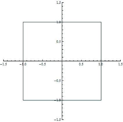
Figure 1: The square region

The statistical problem of the 2-dimensional ideal gas in this region can be solved precisely. We have the spectrum on the square region,

$$E_{n}=\epsilon_{n}=\epsilon_{n_{x},n_{y}}=\frac{\pi^{2}}{4}\left(n_{x}^{2}+n_{y}^{2}\right),$$ (4.1)

and the corresponding wave function is

$$\left|n\right\rangle=\left|n_{x},n_{y}\right\rangle=\sin\left[\frac{n_{x}\pi}{2}\left(x+1\right)\right]\sin\left[\frac{n_{y}\pi}{2}\left(y+1\right)\right].$$ (4.2)

We treat the result of the square region as the zeroth order when we deal with the following examples. We can obtain the partition function of ideal gas on this region, i.e.

$$Z\left(\beta\right) =\sum_{n_{x}}\sum_{n_{y}}\exp\left[-\beta\frac{\pi^{2}}{4}\left(n_{x}^{2}+n_{y}^{2}\right)\right]$$

$$=\frac{1}{4}\left[\vartheta_{3}\left(0,e^{-\frac{1}{4}\pi^{2}\beta}\right)-1\right]^{2},$$ (4.3)

where $\vartheta_{3}\left(0,z\right)$ is Jacobi theta function [24].

We can also calculate several thermodynamic quantities such as the internal energy using the partition function, i.e.[23]

$$U =-\frac{\partial}{\partial\beta}\ln Z\left(\beta\right)$$

$$=\frac{\pi^{2}e^{-\frac{\pi^{2}\beta}{4}}\vartheta_{3}^{(0,1)}\left(0,e^{-\frac{\pi^{2}\beta}{4}}\right)}{2\left[\vartheta_{3}\left(0,e^{-\frac{\pi^{2}\beta}{4}}\right)-1\right]}.$$ (4.4)

The specific heat of the system is given by [23], i.e.

$$C_{V} =\frac{\partial}{\partial T}U=\frac{\partial}{\partial\left(\frac{1}{\beta}\right)}U=\frac{\partial}{\left(-\frac{1}{\beta^{2}}\right)\partial\beta}U$$

$$=\frac{e^{-\frac{\pi^{2}\beta}{2}}\pi^{4}\beta^{2}}{8\left[\vartheta_{3}\left(0,e^{-\frac{\pi^{2}\beta}{4}}\right)-1\right]^{2}}\left\{-\vartheta_{3}^{(0,1)}\left(0,e^{-\frac{\pi^{2}\beta}{4}}\right)^{2}+e^{\frac{\pi^{2}\beta}{4}}\left[\vartheta_{3}\left(0,e^{-\frac{\pi^{2}\beta}{4}}\right)-1\right]\vartheta_{3}^{(0,1)}\left(0,e^{-\frac{\pi^{2}\beta}{4}}\right)\right.$$

$$+\left.\left[\vartheta_{3}\left(0,e^{-\frac{\pi^{2}\beta}{4}}\right)-1\right]\vartheta_{3}^{(0,2)}\left(0,e^{-\frac{\pi^{2}\beta}{4}}\right)\right\}.$$ (4.5)

In the sections that follow we shall consider various cases.

4.1 Transformation of $w=f\left(z\right)=z+\lambda z^{2}$

Let us consider the 2-dimensional regions $\mathcal{D}_{1}$ with complex boundary, Fig. [2]

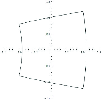
Figure 2: $\lambda=0.1$

where we set $\lambda=0.1$. After conformal transformation, we map the regions $\mathcal{D}_{1}$ onto regions $\Omega$ Fig. [1].

4.1.1 Spectrum of eigenvalue

First, we calculate the conformal factor of the transformation of $w=f\left(z\right)=z+\lambda z^{2}$, i.e.

$$\Sigma=\left|\frac{df}{dz}\right|^{2}=1+4x\lambda+4\lambda^{2}\left(x^{2}+y^{2}\right),$$ (4.6)

then we have

$$\sigma =\Sigma-1$$

$$=4\lambda x+4\lambda^{2}\left(x^{2}+y^{2}\right)$$ (4.7)

Substituting $\sigma$, zero order eigenvalue Eq. (4.1) and zero order eigenfunction Eq. (4.2) into the expression of first order correction to eigenvalue Eq. (2.13), we obtain

$$E_{n}^{\left(1\right)} =-\frac{\pi^{2}}{4}\left(n_{x}^{2}+n_{y}^{2}\right)\int_{-1}^{1}dx\int_{-1}^{1}dy\sin^{2}\left[\frac{n_{x}\pi}{2}\left(x+1\right)\right]\sin^{2}\left[\frac{n_{y}\pi}{2}\left(y+1\right)\right]\left[4\lambda x+4\lambda^{2}\left(x^{2}+y^{2}\right)\right]$$

$$=-\frac{\pi^{2}}{4}\left(n_{x}^{2}+n_{y}^{2}\right)\frac{8}{3}\lambda^{2}\left(1-\frac{3}{\pi^{2}n_{x}^{2}}-\frac{3}{\pi^{2}n_{y}^{2}}\right).$$ (4.8)

4.1.2 Partition function

Now, we calculate the partition function of 2-dimensional ideal gas on the region $\mathcal{D}_{1}$. Substituting the eigenvalue into Eq. (3.2), we have

$$Z\left(\beta\right) =\sum_{\epsilon}e^{-\beta\epsilon}$$

$$=\sum_{n_{x}}\sum_{n_{y}}\exp\left\{-\beta\frac{\pi^{2}}{4}\left(n_{x}^{2}+n_{y}^{2}\right)\left[1-\frac{8}{3}\lambda^{2}\left(1-\frac{3}{\pi^{2}n_{x}^{2}}-\frac{3}{\pi^{2}n_{y}^{2}}\right)\right]\right\}$$ (4.9)

Obviously, it is hard to give an analytical result of the sum, so we can calculate the numerical result of the sum for different $\beta$ (namely different temperature). We calculate the partition function by choosing remove different values of $\beta$. We list numerical results in the Tab. [1],

Table 1: Numerical results

$\beta$	0.01	0.02	0.03	0.04	0.05	0.06	0.07
$Z\left(\beta\right)$	27.158	12.5049	7.80701	5.5305	4.20164	3.33767	2.73481
$\beta$	0.08	0.09	0.10	0.20	0.30	0.40	0.50
$Z\left(\beta\right)$	2.29255	1.95574	1.69171	0.594704	0.288229	0.15799	0.0917356
$\beta$	0.60	0.70	0.80	0.90	1.00
$Z\left(\beta\right)$	0.0547901	0.0331811	0.0202314	0.0123765	0.00758345

In principle, we can give the numerical result for different temperature. But we still give an expression of the partition function based on the table of numerical results. The perturbation calculation is based on the square region $\Omega$, so we can set the partition function on the region $\mathcal{D}_{1}$ as same as the form of the partition function on the square region $\Omega$,

$$Z\left(\beta\right)=\frac{m}{4}\left[\vartheta_{3}\left(0,e^{-\frac{n}{4}\pi^{2}\beta}\right)-1\right]^{2}.$$ (4.10)

Taking the values from the Tab. [1], we give the fitting value of ($m,n$), as

$$m\rightarrow 1.0317,\text{ \ \ \ \ \ \ }n\rightarrow 1.004$$

so we obtain the partition function of 2-dimensional ideal gas on the region $\mathcal{D}_{1}$,

$$Z\left(\beta\right)=\frac{1.0317}{4}\left[\vartheta_{3}\left(0,e^{-\frac{1.004}{4}\pi^{2}\beta}\right)-1\right]^{2}.$$ (4.11)

The internal energy of this system is given by [23], i.e.

$$U =-\frac{\partial}{\partial\beta}\ln Z\left(\beta\right)$$

$$=\frac{1.004\pi^{2}e^{-\frac{1.004}{4}\pi^{2}\beta}\vartheta_{3}^{(0,1)}\left(3,0,e^{-\frac{1.004}{4}\pi^{2}\beta}\right)}{2\left[\vartheta_{3}\left(0,e^{-\frac{1.004}{4}\pi^{2}\beta}\right)-1\right]}.$$ (4.12)

We also have the specific heat of the system [23], i.e.

$$C_{V} =\frac{\partial}{\partial T}U=\frac{\partial}{\partial\left(\frac{1}{\beta}\right)}U=\frac{\partial}{\left(-\frac{1}{\beta^{2}}\right)\partial\beta}U$$

$$=\frac{1.004^{2}e^{-\frac{1.004}{2}\pi^{2}\beta}\pi^{4}\beta^{2}}{8\left[\vartheta_{3}\left(0,e^{-\frac{1.004}{4}\pi^{2}\beta}\right)-1\right]^{2}}\left\{-\vartheta_{3}^{(0,1)}\left(0,e^{-\frac{1.004}{4}\pi^{2}\beta}\right)^{2}+\left[\vartheta_{3}\left(0,e^{-\frac{1.004}{4}\pi^{2}\beta}\right)-1\right]\vartheta_{3}^{(0,2)}\left(0,e^{-\frac{1.004}{4}\pi^{2}\beta}\right)\right.$$

$$\left.+e^{\frac{1.004}{4}\pi^{2}\beta}\left[\vartheta_{3}\left(0,e^{-\frac{1.004}{4}\pi^{2}\beta}\right)-1\right]\vartheta_{3}^{(0,1)}\left(0,e^{-\frac{1.004}{4}\pi^{2}\beta}\right)\right\}.$$ (4.13)

The effect of the thermodynamic quantities after the transformation are shown in the Fig.[3],

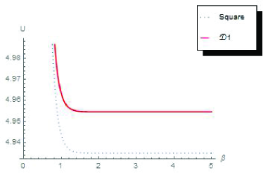
(a) The internal energy

(b) The specific heat

Figure 3: The solid line represent the thermodynamic quantities of the square region, and the dotted line represent the thermodynamic quantities of the $\mathcal{D}_{1}$.

4.2 Transformation of $w=f\left(z\right)=z+\lambda e^{z}$

Let us consider the 2-dimensional regions $\mathcal{D}_{2}$ with complex boundary Fig. [4],

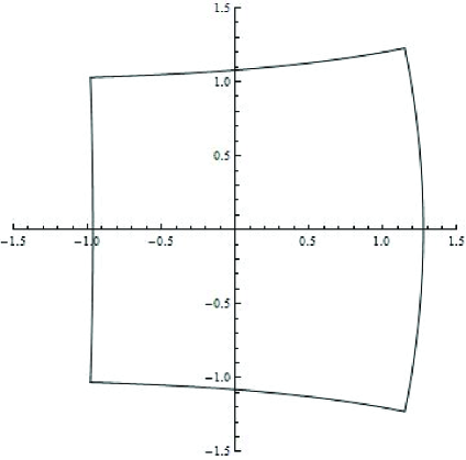
Figure 4: $\lambda=0.1$

where we set $\lambda=0.1$. After conformal transformation, we map the regions $\mathcal{D}_{2}$ onto regions $\Omega$ Fig. [1].

4.2.1 Spectrum of eigenvalue

First, we calculate the conformal factor of transformation of $w=f\left(z\right)=z+\lambda e^{z}$, i.e.

$$\Sigma=\left|\frac{df}{dz}\right|^{2}=1+2e^{x}\lambda\cos y+\lambda^{2}e^{2x},$$ (4.14)

then we have

$$\sigma =\Sigma-1$$

$$=2e^{x}\lambda\cos y+\lambda^{2}e^{2x}.$$ (4.15)

Substituting $\sigma$, zero order eigenvalue Eq. (4.1) and zero order eigenfunction Eq. (4.2) into the expression of first order correction to eigenvalue Eq. (2.13), we obtain

$$E_{n}^{\left(1\right)} =-\frac{\pi^{2}}{4}\left(n_{x}^{2}+n_{y}^{2}\right)\int_{-1}^{1}dx\int_{-1}^{1}dy\sin^{2}\left[\frac{n_{x}\pi}{2}\left(x+1\right)\right]\sin^{2}\left[\frac{n_{y}\pi}{2}\left(y+1\right)\right]\left(2\lambda e^{x}\cos y+\lambda^{2}e^{2x}\right)$$

$$=-\frac{\pi^{2}}{4}\left(n_{x}^{2}+n_{y}^{2}\right)\left[\lambda\frac{\left(e-e^{-1}\right)\pi^{4}n_{x}^{2}n_{y}^{2}\sin 1}{\left(\pi^{2}n_{x}^{2}+1\right)\left(\pi^{2}n_{y}^{2}-1\right)}+\lambda^{2}\frac{\pi^{2}n_{x}^{2}\sinh 2}{2\left(\pi^{2}n_{x}^{2}+4\right)}\right].$$ (4.16)

4.2.2 Partition function

Now, we calculate the partition function of 2-dimensional ideal gas on the region $\mathcal{D}_{2}$. Substituting the eigenvalue into Eq. (3.2), we have

$$Z\left(\beta\right) =\sum_{\epsilon}e^{-\beta\epsilon}$$

$$=\sum_{n_{x}}\sum_{n_{y}}\exp\left[-\beta\frac{\pi^{2}}{4}\left(n_{x}^{2}+n_{y}^{2}\right)\left(1-\lambda\frac{\left(e-e^{-1}\right)\pi^{4}n_{x}^{2}n_{y}^{2}\sin 1}{\left(\pi^{2}n_{x}^{2}+1\right)\left(\pi^{2}n_{y}^{2}-1\right)}-\lambda^{2}\frac{\pi^{2}n_{x}^{2}\sinh 2}{2\left(\pi^{2}n_{x}^{2}+4\right)}\right)\right].$$ (4.17)

Sililar to case 1, we calculate the numerical result of the sum for different $\beta$ and give the numerical results in the Tab. [2],

Table 2: Numerical results

$\beta$	0.01	0.02	0.03	0.04	0.05	0.06	0.07
$Z\left(\beta\right)$	34.458	16.0312	10.0942	7.20541	5.51287	4.40864	3.63556
$\beta$	0.08	0.09	0.10	0.20	0.30	0.40	0.50
$Z\left(\beta\right)$	3.06661	2.63197	2.29021	0.852253	0.437876	0.255918	0.15969
$\beta$	0.60	0.70	0.80	0.90	1.00
$Z\left(\beta\right)$	0.103308	0.0682117	0.0455631	0.0306348	0.020674

Taking the values from the Tab. [2], we obtain the partition function of 2-dimensional ideal gas on the region $\mathcal{D}_{2}$,

$$Z\left(\beta\right)=\frac{1.00614}{4}\left[\vartheta_{3}\left(0,e^{-\frac{0.788871}{4}\pi^{2}\beta}\right)-1\right]^{2}.$$ (4.18)

The internal energy of this system is given by [23], i.e.

$$U =-\frac{\partial}{\partial\beta}\ln Z\left(\beta\right)$$

$$=\frac{0.788871\pi^{2}e^{-\frac{0.788871}{4}\pi^{2}\beta}\vartheta_{3}^{(0,1)}\left(3,0,e^{-\frac{0.788871}{4}\pi^{2}\beta}\right)}{2\left[\vartheta_{3}\left(0,e^{-\frac{0.788871}{4}\pi^{2}\beta}\right)-1\right]}.$$ (4.19)

We also have the specific heat of the system [23], i.e.

$$C_{V} =\frac{\partial}{\partial T}U=\frac{\partial}{\partial\left(\frac{1}{\beta}\right)}U=\frac{\partial}{\left(-\frac{1}{\beta^{2}}\right)\partial\beta}U$$

$$=\!\frac{0.788871^{2}\!e^{-\frac{0.788871}{2}\pi^{2}\beta}\pi^{4}\beta^{2}}{8\!\left[\!\vartheta_{3}\left(0,e^{-\frac{0.788871}{4}\pi^{2}\beta}\right)\!-1\!\right]\!^{2}}\left\{\!-\!\vartheta_{3}^{(0,1)}\left(0,\!e^{-\frac{0.788871}{4}\pi^{2}\beta}\right)^{2}\!+\!\left[\!\vartheta_{3}\left(0,e^{-\frac{0.788871}{4}\pi^{2}\beta}\right)\!-1\!\right]\!\vartheta_{3}^{(0,2)}\!\left(\!0,\!e^{-\frac{0.788871}{4}\pi^{2}\beta}\!\right)\!\right.$$

$$\left.+e^{\frac{0.788871}{4}\pi^{2}\beta}\left[\vartheta_{3}\left(0,e^{-\frac{0.788871}{4}\pi^{2}\beta}\right)-1\right]\vartheta_{3}^{(0,1)}\left(0,e^{-\frac{0.788871}{4}\pi^{2}\beta}\right)\right\}.$$ (4.20)

The effect of the thermodynamic quantities after the transformation are shown in the Fig.[5],

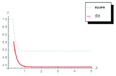
(a) The internal energy

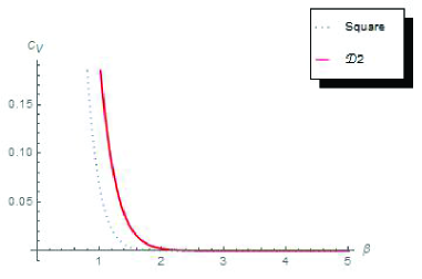
(b) The specific heat

Figure 5: The solid line represent the thermodynamic quantities of the square region, and the dotted line represent the thermodynamic quantities of the $\mathcal{D}_{2}$.

4.3 Transformation of $w=f\left(z\right)=z+\lambda\sin z$

Finally, we consider the 2-dimensional regions $\mathcal{D}_{3}$ with complex boundary Fig. [6] ,

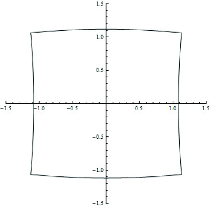
Figure 6: $\lambda=0.1$

where we set $\lambda=0.1$. After conformal transformation, we map the regions $\mathcal{D}_{3}$ onto regions $\Omega$ Fig. [1].

4.3.1 Spectrum of eigenvalue

First, we calculate the conformal factor of the transformation of $w=f\left(z\right)=z+\lambda\sin z$, i.e.

$$\Sigma=\left|\frac{df}{dz}\right|^{2}=1+2\lambda\cos x\cosh y+\frac{1}{2}\lambda^{2}\left(\cos 2x+\cosh 2y\right),$$ (4.21)

then we have

$$\sigma =\Sigma-1$$

$$=2\lambda\cos x\cosh y+\frac{1}{2}\lambda^{2}\left(\cos 2x+\cosh 2y\right).$$ (4.22)

Substituting $\sigma$, zero order eigenvalue Eq. (4.1) and zero order eigenfunction Eq. (4.2) into the expression of first order correction to eigenvalue Eq. (2.13), we obtain

$$E_{n}^{\left(1\right)} =-\frac{\pi^{2}}{4}\left(n_{x}^{2}+n_{y}^{2}\right)\int_{-1}^{1}dx\int_{-1}^{1}dy\sin^{2}\left[\frac{n_{x}\pi}{2}\left(x+1\right)\right]\sin^{2}\left[\frac{n_{y}\pi}{2}\left(y+1\right)\right]$$

$$\times\left[2\lambda\cos x\cosh y+\frac{1}{2}\lambda^{2}\left(\cos 2x+\cosh 2y\right)\right]$$

$$=-\frac{\pi^{2}}{4}\left(n_{x}^{2}+n_{y}^{2}\right)\left[\lambda\frac{\left(e-e^{-1}\right)\pi^{4}n_{x}^{2}n_{y}^{2}\sin 1}{\left(\pi^{2}n_{x}^{2}-1\right)\left(\pi^{2}n_{y}^{2}+1\right)}+\lambda^{2}\frac{\pi^{2}n_{x}^{2}\sin 2}{4\pi^{2}n_{x}^{2}-16}+\lambda^{2}\frac{\pi^{2}n_{y}^{2}\sinh 2}{4\pi^{2}n_{y}^{2}+16}\right].$$ (4.23)

4.3.2 Partition function

Now, we calculate the partition function of 2-dimensional ideal gas on the region $\mathcal{D}_{3}$. Substituting the eigenvalue into Eq. (3.2), we have

$$Z\left(\beta\right) =\sum_{\epsilon}e^{-\beta\epsilon}$$

$$=\sum_{n_{x}}\sum_{n_{y}}\exp\left[-\beta\frac{\pi^{2}}{4}\left(n_{x}^{2}+n_{y}^{2}\right)\left(1-\lambda\frac{\left(e-e^{-1}\right)\pi^{4}n_{x}^{2}n_{y}^{2}\sin 1}{\left(\pi^{2}n_{x}^{2}-1\right)\left(\pi^{2}n_{y}^{2}+1\right)}-\lambda^{2}\frac{\pi^{2}n_{x}^{2}\sin 2}{4\pi^{2}n_{x}^{2}-16}-\lambda^{2}\frac{\pi^{2}n_{y}^{2}\sinh 2}{4\pi^{2}n_{y}^{2}+16}\right)\right]$$ (4.24)

Same as case 1, we calculate the numerical result of the sum for different $\beta$ and give the numerical results in the Tab. [3],

Table 3: Numerical results

$\beta$	0.01	0.02	0.03	0.04	0.05	0.06	0.07
$Z\left(\beta\right)$	34.1644	15.8955	10.0092	7.14507	5.46694	4.37208	3.60555
$\beta$	0.08	0.09	0.10	0.20	0.30	0.40	0.50
$Z\left(\beta\right)$	3.0414	2.61042	2.27152	0.845474	0.434401	0.25384	0.158328
$\beta$	0.60	0.70	0.80	0.90	1.00
$Z\left(\beta\right)$	0.102364	0.0675327	0.0450658	0.0302677	0.0204026

Taking the values from the Tab. [3], we obtain the partition function of 2-dimensional ideal gas on the region $\mathcal{D}_{3}$,

$$Z\left(\beta\right)=\frac{0.996072}{4}\left[\vartheta_{3}\left(0,e^{-\frac{0.787783}{4}\pi^{2}\beta}\right)-1\right]^{2}.$$ (4.25)

The internal energy of this system is given by [23], i.e.

$$U =-\frac{\partial}{\partial\beta}\ln Z\left(\beta\right)$$

$$=\frac{0.787783\pi^{2}e^{-\frac{0.787783}{4}\pi^{2}\beta}\vartheta_{3}^{(0,1)}\left(3,0,e^{-\frac{0.787783}{4}\pi^{2}\beta}\right)}{2\left[\vartheta_{3}\left(0,e^{-\frac{0.787783}{4}\pi^{2}\beta}\right)-1\right]}.$$ (4.26)

We also have the specific heat of the system [23], i.e.

$$C_{V} =\frac{\partial}{\partial T}U=\frac{\partial}{\partial\left(\frac{1}{\beta}\right)}U=\frac{\partial}{\left(-\frac{1}{\beta^{2}}\right)\partial\beta}U$$

$$\!=\!\frac{0.787783^{2}\!e^{-\frac{0.787783}{2}\pi^{2}\beta}\pi^{4}\beta^{2}}{8\!\left[\!\vartheta_{3}\left(0,\!e^{-\frac{0.787783}{4}\pi^{2}\beta}\right)-1\!\right]^{2}}\left\{\!-\vartheta_{3}^{(0,1)}\left(0,\!e^{-\frac{0.787783}{4}\pi^{2}\beta}\right)^{2}+\!\left[\!\vartheta_{3}\left(0,\!e^{-\frac{0.787783}{4}\pi^{2}\beta}\!\right)\!-1\!\right]\!\vartheta_{3}^{(0,2)}\left(0,\!e^{-\frac{0.787783}{4}\pi^{2}\beta}\right)\right.$$

$$\left.+e^{\frac{0.787783}{4}\pi^{2}\beta}\left[\vartheta_{3}\left(0,e^{-\frac{0.787783}{4}\pi^{2}\beta}\right)-1\right]\vartheta_{3}^{(0,1)}\left(0,e^{-\frac{0.787783}{4}\pi^{2}\beta}\right)\right\}.$$ (4.27)

The effect of the thermodynamic quantities after the transformation are shown in the Fig.[7],

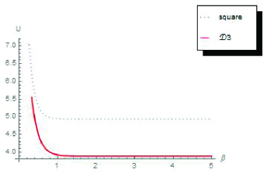
(a) The internal energy

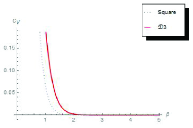
(b) The specific heat

Figure 7: The solid line represent the thermodynamic quantities of the square region, and the dotted line represent the thermodynamic quantities of the $\mathcal{D}_{3}$.

5 Conclusion

In this paper, based on the conformal mapping method and perturbation theory, we present an approach to solve the statistical problem of ideal gas within general 2-dimensional regions. We considered some example and give numerical results. For more general case, we can state the transformation as follow:

$$f\left(z\right)=z+\sum\lambda_{n}z^{n}+\sum\alpha_{n}e^{nz}+\sum\beta_{n}\sin nz.$$ (5.1)

Then we obtain the transformation by calculating the undetermined parameters $\lambda_{n}$, $\alpha_{n}$ and $\beta_{n}$. Using the approach given in this paper, we are able to solve the statistical problem of ideal gas in general 2-dimensional regions.

References

- [1] M. Robnik, Quantising a generic family of billiards with analytic boundaries Journal of Physics A: Mathematical and General 17 (1984), No. 5 1049.
- [2] P. Amore, Spectroscopy of drums and quantum billiards: Perturbative and nonperturbative results Journal of Mathematical Physics 51 (2010), No. 5 052105.
- [3] L. A. Segel, Application of conformal mapping to viscous flow between moving circular cylinders Quarterly of Applied Mathematics 18 (1961), No. 4 335–353.
- [4] L. A. Segel, Application of conformal mapping to boundary perturbation problems for the membrane equation Archive for Rational Mechanics and Analysis 8 (1961), No. 1 228–237.
- [5] K. Kodaira, A. Beardon, and T. Carne, Complex Analysis. Cambridge Studies in Advanced Mathematics. Cambridge University Press, 2007.
- [6] A. Sisman and I. Muller, The Casimir-like size effects in ideal gases Physics Letters A 320 (2004), No. 5 360–366.
- [7] A. Sisman, Surface dependency in thermodynamics of ideal gases Journal of Physics A: Mathematical and General 37 (2004), No. 47 11353.
- [8] A. Sisman, Z. Ozturk, and C. Firat, Quantum boundary layer: a non-uniform density distribution of an ideal gas in thermodynamic equilibrium Physics Letters A 362 (2007), No. 1 16–20.
- [9] C. Firat and A. Sisman, Universality of the quantum boundary layer for a Maxwellian gas Physica Scripta 79 (2009), No. 6 065002.
- [10] W.-S. Dai and M. Xie, Quantum statistics of ideal gases in confined space Physics Letters A 311 (2003), No. 4 340–346.
- [11] W.-S. Dai and M. Xie, Geometry effects in confined space Physical Review E 70 (2004), No. 1 016103.
- [12] W. Dai and M. Xie, Hard-sphere gases as ideal gases with multi-core boundaries: An approach to two-and three-dimensional interacting gases EPL (Europhysics Letters) 72 (2005), No. 6 887.
- [13] W.-S. Dai and M. Xie, Interacting quantum gases in confined space: Two-and three-dimensional equations of state Journal of Mathematical Physics 48 (2007), No. 12 123302.
- [14] H. Pang, W.-S. Dai, and M. Xie, The difference of boundary effects between Bose and Fermi systems Journal of Physics A: Mathematical and General 39 (2006), No. 11 2563.
- [15] Z. Huang, C. Ou, A. L. Méhauté, Q. A. Wang, and J. Chen, Inherent correlations between thermodynamics and statistical physics in extensive and nonextensive systems Physica A: Statistical Mechanics and its Applications 388 (2009), No. 12 2331–2336.
- [16] W.-S. Dai and M. Xie, The number of eigenstates: counting function and heat kernel Journal of High Energy Physics 2009 (2009), No. 02 033.
- [17] W.-S. Dai and M. Xie, An approach for the calculation of one-loop effective actions, vacuum energies, and spectral counting functions Journal of High Energy Physics 2010 (2010), No. 6 1–29.
- [18] Z. Ozturk and A. Sisman, Quantum size effects on the thermal and potential conductivities of ideal gases Physica Scripta 80 (2009), No. 6 065402.
- [19] G. Su and J. Chen, Bose–Einstein condensation of a finite-size Bose system European Journal of Physics 31 (2010), No. 1 143.
- [20] W. Nie and J. He, Performance analysis of a thermosize micro/nano heat engine Physics Letters A 372 (2008), No. 8 1168–1173.
- [21] W. Nie, J. He, and J. Du, Performance characteristic of a Stirling refrigeration cycle in micro/nano scale Physica A: Statistical Mechanics and its Applications 388 (2009), No. 4 318–324.
- [22] W. Nie and J. He, Quantum boundary effect on the work output of a micro-/nanoscaled Carnot cycle Journal of Applied Physics 105 (2009), No. 5 054903–054903.
- [23] R. K. Pathria, Statistical Mechanics. Butterworth Heineman, Oxford, UK, second ed., 1996.
- [24] M. Abramowitz and I. A. Stegun, Handbook of mathematical functions: with formulas, graphs, and mathematical tables. Courier Dover Publications, 2012.