Form factors of the transitions in the covariant quark model
Abstract
In the wake of exploring uncertainty in the full angular distribution of the decay caused by the presence of the intermediate scalar meson, we perform the straightforward calculation of the ( is a scalar meson) transition form factors in the full kinematical region within the covariant quark model. We restrict ourselves to the scalar mesons below 1 GeV: , , , and . As an application of the obtained results we calculate the widths of the semileptonic and rare decays , and . We compare our results with those obtained in other approaches.
pacs:
12.39.Ki,13.30.Eg,14.20.Jn,14.20.MrI Introduction
Recently, much attention has been paid to the rare flavor-changing neutral current decay . One of the reasons for this was the first measurement of form-factor-independent angular observables performed by the LHCb Collaboration Aaij:2013qta ; Aaij:2013iag . It has been claimed that there is a 3.7 deviation from the Standard Model (SM) prediction for one of the angular observables. Much effort has been spent to explain this deviation by invoking the effects of new physics (NP) (for example, see Refs. Hurth:2013ssa ; Descotes-Genon:2013vna ; Datta:2013kja ; Bobeth:2012vn ; Altmannshofer:2013foa ; Altmannshofer:2014rta ; Mandal:2014kma and references therein). The main emphasis of the above-mentioned papers was on the search for the physical observables that have low sensitivity to the form factors.
In addition to the NP effects, the uncertainties related to the presence of the intermediate scalar resonance decaying into have been intensively discussed in the literature Lu:2011jm ; Doring:2013wka ; Meissner:2013pba ; Becirevic:2012dp ; Matias:2012qz ; Blake:2012mb ; Das:2014sra . A detailed analysis of the decay in the higher kaon resonance region was done in Ref. Lu:2011jm . In many papers, the Breit-Wigner form for the mass spectra was used. However, this assumption cannot be justified for the broad scalar resonances like the meson. The improvement of the description was done in Ref. Doring:2013wka by invoking the chiral perturbation theory for the interaction. This issue was also generalized to in Ref. Meissner:2013pba .
As is well-known, short-distance physics is under control in the description of the rare decays, whereas the effects of long-distance physics described by the hadronic form factors lead to large uncertainties since they involve nonperturbative QCD. The calculation of the transition form factors have been performed in many theoretical approaches and models. We must mention some of them: light-cone QCD sum rules Ali:1999mm , QCD sum rules Colangelo:1995jv , the lattice-constrained dispersion quark model Melikhov:1997wp , the simple dipole parametrization Aliev:2001fc , perturbative QCD at large recoil region Chen:2002bq , the relativistic quark model Ebert:2010dv , and the Dyson-Schwinger equations in QCD Ivanov:2007cw .
The and to transition form factors were calculated in Ref. Yang:2005bv within an approach based on QCD sum rules. The form factors for the transition have been evaluated in the light-front quark model Chen:2007na . The form factors of rare decay were calculated in Ref. Aliev:2007rq within three-point QCD sum rules. The transition form factors have been investigated in the light-cone sum rules approach Wang:2008da . The transition form factors of -mesons decay into a scalar meson were studied in Ref. Li:2008tk within the perturbative QCD approach. With these form factors, the decay width and branching ratios of the semileptonic and rare decays have been calculated. The rare semileptonic decays and were investigated in Ref. Ghahramany:2009zz in the framework of the three-point QCD sum rules. The transition form factors were computed in Ref. Colangelo:2010bg by using light-cone QCD sum rules at leading order in the strong coupling constant and an estimate of next-to-leading-order corrections. A QCD light-cone sum rule was also used to evaluate the form factors and branching ratios in Ref. Sun:2010nv . The twist-3 light-cone distribution amplitudes (LCDAs) of the scalar mesons were investigated in Ref. Han:2013zg within the QCD sum rules. As an application of those twist-3 LCDAs, the transition form factors were studied by introducing proper chiral currents into the correlator.
Recently, the form factors for two scalar nonet mesons below and above 1 GeV were calculated in Ref. Wang:2014vra by taking into account the perturbative corrections to the twist-2 terms using the light-cone QCD sum rules. They were used in Ref. Wang:2014upa to study the semileptonic and rare decays.
In the wake of exploring uncertainty in the full angular distribution of the decay caused by the presence of the intermediate scalar meson, we perform the straightforward calculation of the ( is a scalar meson) transition form factors in the full kinematical region within the covariant quark model. We restrict ourselves to the scalar mesons below 1 GeV: , , , and Agashe:2014kda . Actually, the internal structure of these mesons is not yet well established (see Refs. Amsler:2013wea ; Amsler:2004ps for a review). We will use the simple interpretation of the low-lying scalar mesons in our calculation. The calculated form factors are used to evaluate the branching fractions of the decay , where . We compare our results with those obtained in other approaches.
The paper is organized in the following manner. In Sec. II we give the necessary theoretical framework which includes the effective Hamiltonian, its matrix element between the initial and final states, the definition of the hadronic form factors and the helicity amplitudes. In Sec. III we briefly discuss our covariant quark model and calculate the form factors of the transitions and . Finally, we present our numerical results for the differential decay distributions and branching ratios. We compare our findings with the results of other approaches.
II Effective Hamiltonian and form factors
We start with the on-shell decays which can be described by using the effective Hamiltonian for the transition Buras:1994dj ; Buchalla:1995vs . The effective Hamiltonian leads to the free-quark decay amplitude:
| (1) | |||||
where is the weak Dirac matrix, is the product of the Cabibbo-Kobayashi-Maskawa elements, and . The Wilson coefficient effectively takes into account (i) the contributions from the four-quark operators and (ii) the nonperturbative effects coming from the -resonance contributions which are as usual parametrized by a Breit-Wigner ansatz Ali:1991is :
| (2) | |||||
where , , and . Here
| (5) | |||||
where is a scale parameter and . In what follows, we will not include the long-distance contributions coming from the and resonances Ali:1991is and charm-loop effects Khodjamirian:2010vf .
We specify our choice of the momenta as with , and where and are the and momenta, and , , are the masses of the initial meson , the final meson , and the lepton , respectively. The matrix elements of the exclusive transitions are defined by
| (6) | |||||
where , .
We define dimensionless form factors by
| (7) |
where and . The matrix element in Eq (6) is written as
where the quantities are expressed through the form factors and the Wilson coefficients in the case of the spinless particle as
| (8) |
Respectively, the helicity form factors are defined in terms of the invariant form factors as Faessler:2002ut
| (9) |
The differential two-fold decay distribution may be written in terms of the bilinear combinations of the helicity amplitudes (see Ref. Faessler:2002ut ). However, it is common in the modern literature to use the transversality amplitudes and defined in Ref. Kruger:2005ep . They are related to our helicity amplitudes by
| (10) |
where the overall factor is given by
where is the momentum of the outgoing meson and is the lepton velocity, both of which are given in the rest frame of the parent meson .
The differential decay distribution then reads
| (11) | |||||
Integrating over one obtains
| (12) | |||||
where we have introduced a flip parameter .
We also calculate the differential rates for the semileptonic mode and rare decay. One has
III The transition form factors in the covariant quark model
We calculate the transition form factors in the covariant quark model. We briefly recall the basic features of this approach, which was formulated in its modern form in Ref. Branz:2009cd by taking into account the infrared confinement of quarks.
The model is based on an effective interaction Lagrangian describing the coupling of hadrons to their constituent quarks. For instance, the coupling of a meson to its constituent quarks and is described by the nonlocal Lagrangian
| (15) |
Here, is the Dirac matrix, which is chosen appropriately to describe the spin quantum numbers of the meson field . The vertex function characterizes the finite size of the meson. To satisfy translational invariance the vertex function has to obey the identity for any given four-vector . We use a specific form for the vertex function which satisfies the above translation invariance relation. One has
| (16) |
where is the correlation function of the two constituent quarks with masses and . The variable is defined by , so that . We choose a simple Gaussian form for the vertex function . The minus sign in the argument of is chosen to emphasize that we are working in Minkowski space. One has
| (17) |
where the parameter characterizes the size of the meson. Since turns into in Euclidean space the form (17) has the appropriate falloff behavior in the Euclidean region. We stress that any choice for is appropriate as long as it falls off sufficiently fast in the ultraviolet region of Euclidean space in order to render the Feynman diagrams ultraviolet finite.
In the evaluation of the quark-loop diagrams we use the free local fermion propagator for the constituent quark,
| (18) |
with an effective constituent quark mass .
The coupling constant in Eq. (15) is determined by the so-called compositeness condition suggested by Weinberg Weinberg:1962hj and Salam Salam:1962ap (for a review, see Ref. Hayashi:1967hk ) and extensively used in our studies (for details, see Ref. Efimov:1993ei ). The compositeness condition requires that the renormalization constant of the elementary meson field is set to zero, i.e.,
| (19) |
where is the derivative of the mass operator corresponding to the self–energy diagram in Fig. 1.
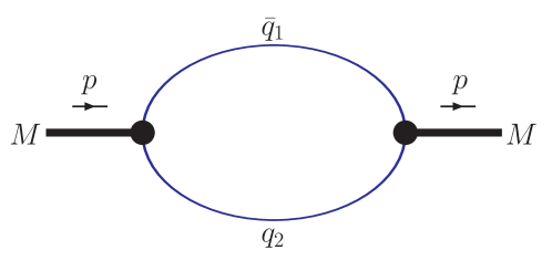
To clarify the physical meaning of the compositeness condition, we recall that the renormalization constant can also be interpreted as the matrix element between the physical state and the corresponding bare state. For it then follows that the physical state does not contain the bare one and it is therefore described as a bound state. The interaction Lagrangian (15) and the corresponding free Lagrangian describe both the constituents (quarks) and the physical particles (hadrons), which are bound states of the constituents. As a result of the interaction, the physical particle is dressed, i.e., its mass and wave function have to be renormalized. The condition also effectively excludes the constituent degrees of freedom from the space of physical states and thereby guarantees that there will be no double counting. The constituents exist in virtual states only.
The covariant quark model was applied to evaluate the form factors of the transitions in the full kinematical region of momentum transfer squared Ivanov:2011aa ; Dubnicka:2013vm This approach was extended to describe the baryons as three-quark states baryon and the exotic meson X(3872) as a tetraquark tetraquark .
A similar approach based on the compositeness condition was recently developed in Ref. Cheung:2014cka .
In this paper we evaluate the transition form factors assuming that the scalar mesons below 1 GeV are ordinary two-quark states. Some remarks should be made before performing the calculations. The internal structure of the light scalar mesons is not yet well established (for review, see Refs. Amsler:2013wea ; Amsler:2004ps ). Since they have large decay widths it is difficult to distinguish them from background. There are interpretations of these objects as four-quark states and/or gluballs. Here, we describe the scalar mesons as two-quark states and evaluate the form factors within our approach, but when we use the calculated form factors in the matrix element of the cascade decay we take into account the line shape of the , which reflects the broad width of this resonance. One can also describe the scalar mesons as four-quark states in our approach, similar to the exotic meson X(3872) tetraquark ; however, this is beyond the scope of this work.
The SU(3) nonet of scalar mesons below 1 GeV can be written in the matrix form
| (20) |
The physical scalar fields are related to the Cartesian basis in the following manner:
| (21) |
where is the octet-singlet mixing angle. The vertex is then written as
| (22) | |||||
where , with the ideal mixing angle . We will use the notation from Ref. Agashe:2014kda for the scalar mesons below 1 GeV:
-
•
, , MeV;
-
•
, , MeV;
-
•
, , MeV;
-
•
, , MeV.
Moreover, we assume that , i.e., to ensure a pure state.
The coupling constant in Eq. (15) is determined by Eq. (19), where is the derivative of the scalar meson mass operator,
| (23) | |||||
By using the calculation technique outlined in Ref. Branz:2009cd , one can easily perform the loop integration. We give the analytic result for equal quark masses ():
| (24) | |||||
Note that in the case of the branching point appears at . At this point the integral over becomes divergent as because at . By introducing an infrared cutoff on the upper limit of the scale of integration, one can avoid the appearance of the threshold singularity.
Herein our primary subjects are the transition matrix elements, which can be expressed via the dimensionless form factors defined in Refs. Ivanov:2011aa ; Dubnicka:2013vm . The diagram corresponding to these matrix elements is shown in Fig. 2.
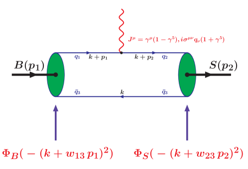
One has
| (26) |
Here, , , , and . Since there are three sorts of quarks involved in these processes, we introduce the notation with two subscripts, so that .
The first fit of the model parameters was done in the original paper Branz:2009cd , where the infrared quark confinement was implemented for the first time. The leptonic decay constants (which are known either from experiments or from lattice simulations) have been chosen as the input quantities to adjust the model parameters. A given meson in the interaction Lagrangian is characterized by the coupling constant , the size parameter and two of the four constituent quark masses, (, , , ). Moreover, there is the infrared confinement parameter , which is universal for all hadrons. Note that the physical values for the hadron masses have been used in the fit. Therefore, one has adjustable parameters for numbers of mesons. The compositeness condition provides constraints and allows one to express all coupling constants via other model parameters. The remaining parameters are determined by a fit to experimental data. The values of leptonic decay constants and some electromagnetic decay widths have been chosen as the input data. Several updated fits were done in Refs. Ivanov:2011aa ; Dubnicka:2013vm . In this paper we will use the latest fit done in Ref. Ganbold:2014pua . The fitted values of the constituent quark masses , the infrared cut-off , and the size parameters are given by Eq. (27) and Table 1.
| (27) |
| 0.87 | 1.02 | 1.71 | 1.81 | 1.96 | 2.05 | 2.50 | 2.06 | 2.95 | |
| 0.61 | 0.50 | 0.91 | 1.93 | 0.75 | 1.51 | 1.71 | 1.76 | 1.71 | 2.96 |
Our form factors are represented as three-fold integrals which are calculated by using NAG routines. The results of our numerical calculations are well approximated by the parametrization
| (28) |
We consider the following weak transitions: (charged current), and and (flavor-changing neutral currents). The values of , , and are listed in Table 2.
| 0.144 | 1.624 | 0.585 | 0.192 | 1.433 | 0.381 | ||
| 0.138 | 1.667 | 0.674 | 0.274 | 1.258 | 0.292 | ||
| 0.141 | 1.663 | 0.651 | 0.254 | 1.269 | 0.262 | ||
| 0.191 | 1.348 | 0.407 | 0.306 | 0.988 | 0.108 | ||
| 0.120 | 1.448 | 0.485 | 0.210 | 1.067 | 0.155 | ||
| 0.049 | 2.144 | 1.196 | 0.089 | 1.723 | 0.688 | ||
| 0.138 | 1.727 | 0.734 | 0.268 | 1.291 | 0.310 | ||
| 0.140 | 1.761 | 0.755 | 0.253 | 1.320 | 0.295 | ||
| 0.199 | 1.406 | 0.457 | 0.296 | 1.032 | 0.129 | ||
| 0.116 | 1.504 | 0.536 | 0.191 | 1.110 | 0.180 | ||
| 0.165 | 1.680 | 0.667 | 0.285 | 1.276 | 0.257 | ||
| 0.206 | 1.367 | 0.423 | 0.306 | 1.005 | 0.113 | ||
| 0.124 | 1.460 | 0.496 | 0.203 | 1.080 | 0.159 | ||
IV Numerical results and discussion
We use the following set of SM parameters: GeV-2, GeV, GeV, GeV, GeV, , , , a scale parameter , and the Wilson coefficients , , , , , , , , and . We take the average values of the hadron and lepton masses and the -meson lifetimes from Ref. Agashe:2014kda .
All model parameters are fixed by fitting the experimental data in our previous papers (see Refs. Ivanov:2011aa ; Dubnicka:2013vm ; Ganbold:2014pua ; baryon ). Their numerical values are shown in Eq. (27) and Table 1. The only new parameter is which characterizes the size of the scalar mesons. We allow this parameter to vary in a relatively large interval, GeV.
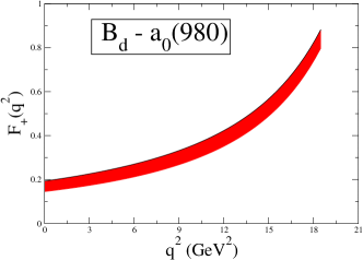
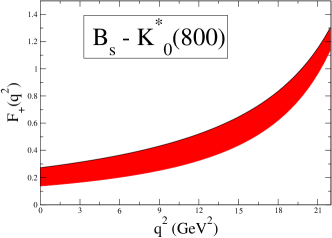
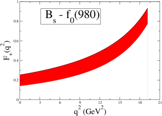
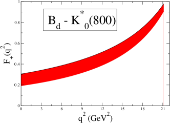
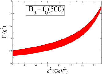
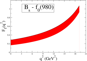
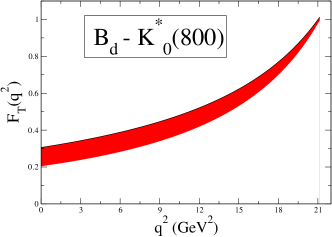
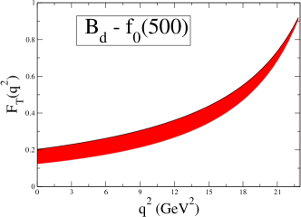
In Figs. 3 and 4, we plot our calculated and form factors in the entire kinematical range . Since the behavior of is very similar to that of , we do not display them. One can see that the form factors are more sensitive to the choice of at small and less so near zero recoil.
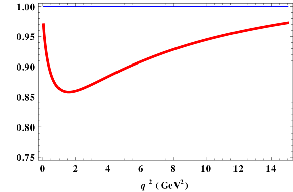
We are going to explore the influence of the intermediate scalar meson on the angular decay distribution of the cascade decay . Therefore, we give the maximum values of the form factors in Table 3 and the branching ratios in Table 4 obtained for GeV. The results for the mode are almost identical to those of the mode and will not be shown separately. Since the ratio is relatively small we do not show the branching ratios of the decays with the transition. We compare the obtained results with those from other approaches. One can see that our values for the branching ratios are almost half of those from other approaches.
Let us briefly discuss the impact of the scalar resonance on decay. As is well known, the narrow vector resonance is described by a Breit-Wigner parametrization and the given cascade decay can be calculated by using the narrow-width approximation. But this is not true in the case of the broad scalar meson. There are several parametrizations of the line shapes in the literature; see, for instance, the discussion in Ref. Doring:2013wka . For the time being we will use the parametrization accepted in Ref. Meissner:2013pba , the integrated value of which in the -resonance region is equal to
| (29) |
Then, we scale the calculated value for the differential decay rate by this factor and compare it with that for decay. We display the behavior of the ratio
| (30) |
in Fig.5, which may be compared with the finding of Ref. Becirevic:2012dp . The integrated ratio (the numerator and denominator are integrated separately in the full kinematical region of ) gives a size for the -wave pollution to the branching ratio of the decay of about 6.
| This work | Wang:2014vra | Sun:2010nv | Colangelo:1995jv | Li:2008tk | Ghahramany:2009zz | ElBennich:2008xy | ||
| 0.192 | 0.58 | 0.56 | ||||||
| 0.274 | 0.44 | 0.53 | ||||||
| 0.254 | 0.45 | 0.44 | 0.19 | 0.35 | 0.12 | 0.40 | ||
| 0.285 | 0.60 | 0.58 | 0.23 | 0.40 | -0.08 | |||
| 0.306 | 0.50 | 0.46 | ||||||
| 0.306 | 0.67 | 0.58 | ||||||
| 0.210 | ||||||||
| 0.203 |
| Decay modes | Branching fractions | |||
|---|---|---|---|---|
| This work | Wang:2014upa | Colangelo:1995jv | Li:2008tk | |
| ( GeV) | ||||
.
Acknowledgments
We thank Pietro Santorelli for providing us with the last fit of the parameters in the covariant quark model. We would also like to thank Juergen Körner and Valery Lyubovitskij for many useful discussions of -physics facets related to the subject of this paper. We are grateful to Wei Wang and David Straub for pointing out the relevant references.
References
- (1) R. Aaij et al. [LHCb Collaboration], Phys. Rev. Lett. 111, 191801 (2013) [arXiv:1308.1707 [hep-ex]].
- (2) R. Aaij et al. [LHCb Collaboration], J. High Energy Phys. 08 (2013) 131 [arXiv:1304.6325 [hep-ex]].
- (3) T. Hurth and F. Mahmoudi, J. High Energy Phys. 04 (2014) 097 [arXiv:1312.5267 [hep-ph]].
- (4) S. Descotes-Genon, T. Hurth, J. Matias and J. Virto, J. High Energy Phys. 05 (2013) 137 [arXiv:1303.5794 [hep-ph]].
- (5) A. Datta, M. Duraisamy and D. Ghosh, Phys. Rev. D 89, 071501 (2014) [arXiv:1310.1937 [hep-ph]].
- (6) C. Bobeth, G. Hiller, and D. van Dyk, Phys. Rev. D 87, 034016 (2013) [arXiv:1212.2321 [hep-ph]].
- (7) W. Altmannshofer and D. M. Straub, Eur. Phys. J. C 73, 2646 (2013) [arXiv:1308.1501 [hep-ph]].
- (8) W. Altmannshofer and D. M. Straub, State of new physics in transitions, [arXiv:1411.3161 [hep-ph]].
- (9) R. Mandal, R. Sinha, and D. Das, Phys. Rev. D 90, 096006 (2014) [arXiv:1409.3088 [hep-ph]].
- (10) C. D. Lu and W. Wang, Phys. Rev. D 85, 034014 (2012) [arXiv:1111.1513 [hep-ph]].
- (11) M. Döring, U. G. Meissner, and W. Wang, J. High Energy Phys. 10 (2013) 011 [arXiv:1307.0947 [hep-ph]].
- (12) U. G. Meissner and W. Wang, J. High Energy Phys. 01 (2014) 107 [arXiv:1311.5420 [hep-ph]].
- (13) D. Becirevic and A. Tayduganov, Nucl. Phys. B868, 368 (2013) [arXiv:1207.4004 [hep-ph]].
- (14) J. Matias, Phys. Rev. D 86, 094024 (2012) [arXiv:1209.1525 [hep-ph]].
- (15) T. Blake, U. Egede, and A. Shires, J. High Energy Phys. 03 (2013) 027 [arXiv:1210.5279 [hep-ph]].
- (16) D. Das, G. Hiller, M. Jung, and A. Shires, J. High Energy Phys. 09 (2014) 109 [arXiv:1406.6681 [hep-ph]].
- (17) A. Ali, P. Ball, L. T. Handoko, and G. Hiller, Phys. Rev. D 61, 074024 (2000) [hep-ph/9910221].
- (18) P. Colangelo, F. De Fazio, P. Santorelli, and E. Scrimieri, Phys. Rev. D 53, 3672 (1996); Phys. Rev. D 57, 3186(E) (1998)
- (19) D. Melikhov, N. Nikitin, and S. Simula, Phys. Rev. D 57, 6814 (1998)
- (20) T. M. Aliev, A. Ozpineci, and M. Savci, Phys. Lett. B 511, 49 (2001)
- (21) C. H. Chen and C. Q. Geng, Nucl. Phys. B636, 338 (2002)
- (22) D. Ebert, R. N. Faustov, and V. O. Galkin, Phys. Rev. D 82, 034032 (2010) [arXiv:1006.4231 [hep-ph]].
- (23) M. A. Ivanov, J. G. Körner, S. G. Kovalenko, and C. D. Roberts, Phys. Rev. D 76, 034018 (2007)
- (24) K. A. Olive et al. [Particle Data Group Collaboration], Chin. Phys. C 38, 090001 (2014).
- (25) C. Amsler, S. Eidelman, T. Gutsche, C. Hanhart, S. Spanier, and N. A. Tornqvist, Note on Scalar Mesons below 2 GeV in Ref. Agashe:2014kda .
- (26) C. Amsler and N. A. Tornqvist, Phys. Rep. 389, 61 (2004).
- (27) M. Z. Yang, Phys. Rev. D 73, 034027 (2006); Phys. Rev. D 73, 079901(E) (2006)
- (28) C. H. Chen, C. Q. Geng, C. C. Lih, and C. C. Liu, Phys. Rev. D 75, 074010 (2007)
- (29) T. M. Aliev, K. Azizi, and M. Savci, Phys. Rev. D 76, 074017 (2007) [arXiv:0710.1508 [hep-ph]].
- (30) Y. M. Wang, M. J. Aslam, and C. D. Lu, Phys. Rev. D 78, 014006 (2008) [arXiv:0804.2204 [hep-ph]].
- (31) R. H. Li, C. D. Lu, W. Wang, and X. X. Wang, Phys. Rev. D 79, 014013 (2009) [arXiv:0811.2648 [hep-ph]].
- (32) N. Ghahramany and R. Khosravi, Phys. Rev. D 80, 016009 (2009).
- (33) P. Colangelo, F. De Fazio, and W. Wang, Phys. Rev. D 81, 074001 (2010) [arXiv:1002.2880 [hep-ph]].
- (34) Y. J. Sun, Z. H. Li, and T. Huang, Phys. Rev. D 83, 025024 (2011) [arXiv:1011.3901 [hep-ph]].
- (35) H. Y. Han, X. G. Wu, H. B. Fu, Q. L. Zhang, and T. Zhong, Eur. Phys. J. A 49, 78 (2013) [arXiv:1301.3978 [hep-ph]].
- (36) Z. G. Wang, Eur. Phys. J. C 75, 50 (2015) [arXiv:1409.6449 [hep-ph]].
- (37) Z. G. Wang, Semi-leptonic decays in the standard model and in the universal extra dimension model, [arXiv:1411.7961 [hep-ph]].
- (38) A. J. Buras and M. Munz, Phys. Rev. D 52, 186 (1995) [hep-ph/9501281].
- (39) G. Buchalla, A. J. Buras, and M. E. Lautenbacher, Rev. Mod. Phys. 68, 1125 (1996) [hep-ph/9512380].
- (40) A. Ali, T. Mannel, and T. Morozumi, Phys. Lett. B 273, 505 (1991).
- (41) A. Khodjamirian, T. Mannel, A. A. Pivovarov, and Y.-M. Wang, J. High Energy Phys. 09, (2010) 089 [arXiv:1006.4945 [hep-ph]].
-
(42)
A. Faessler, T. Gutsche, M. A. Ivanov, J. G. Körner, and V. E. Lyubovitskij,
Eur. Phys. J. direct C 4, 18 (2002) [hep-ph/0205287]. - (43) F. Kruger and J. Matias, Phys. Rev. D 71, 094009 (2005) [hep-ph/0502060].
- (44) T. Branz, A. Faessler, T. Gutsche, M. A. Ivanov, J. G. Körner, and V. E. Lyubovitskij, Phys. Rev. D 81, 034010 (2010) [arXiv:0912.3710 [hep-ph]].
- (45) S. Weinberg, Phys. Rev. 130, 776 (1963).
- (46) A. Salam, Nuovo Cimento 25, 224 (1962).
- (47) K. Hayashi, M. Hirayama, T. Muta, N. Seto, and T. Shirafuji, Fortsch. Phys. 15, 625 (1967).
- (48) G. V. Efimov and M. A. Ivanov, The Quark Confinement Model of Hadrons, (CRC Press, Boca Raton, 1993).
- (49) M. A. Ivanov, J. G. Körner, S. G. Kovalenko, P. Santorelli, and G. G. Saidullaeva, Phys. Rev. D 85, 034004 (2012) [arXiv:1112.3536 [hep-ph]].
- (50) S. Dubnicka, A. Z. Dubnickova, M. A. Ivanov, and A. Liptaj, Phys. Rev. D 87, 074201 (2013) [arXiv:1301.0738 [hep-ph]].
- (51) T. Gutsche, M. A. Ivanov, J. G. Körner, V. E. Lyubovitskij, and P. Santorelli, Phys. Rev. D 86, 074013 (2012) [arXiv:1207.7052 [hep-ph]]; Phys. Rev. D 87, 074031 (2013) [arXiv:1301.3737 [hep-ph]]; Phys. Rev. D 88, no. 11, 114018 (2013) [arXiv:1309.7879 [hep-ph]]; Phys. Rev. D 90, no. 11, 114033 (2014) [arXiv:1410.6043 [hep-ph]].
- (52) S. Dubnicka, A. Z. Dubnickova, M. A. Ivanov, and J. G. Körner, Phys. Rev. D 81, 114007 (2010) [arXiv:1004.1291 [hep-ph]]; S. Dubnicka, A. Z. Dubnickova, M. A. Ivanov, J. G. Koerner, P. Santorelli, and G. G. Saidullaeva, Phys. Rev. D 84, 014006 (2011) [arXiv:1104.3974 [hep-ph]].
- (53) C. Y. Cheung and C. W. Hwang, J. High Energy Phys. 04, (2014) 177 [arXiv:1401.3917 [hep-ph]].
- (54) G. Ganbold, T. Gutsche, M. A. Ivanov, and V. E. Lyubovitskij, On the meson mass spectrum in the covariant confined quark model, [arXiv:1410.3741 [hep-ph]].
- (55) B. El-Bennich, O. Leitner, J.-P. Dedonder, and B. Loiseau, Phys. Rev. D 79, 076004 (2009) [arXiv:0810.5771 [hep-ph]].
 |
|
 |
|
 |
 |
|
 |