How predictable is technological progress?

Abstract

Recently it has become clear that many technologies follow a generalized version of Moore’s law, i.e. costs tend to drop exponentially, at different rates that depend on the technology. Here we formulate Moore’s law as a correlated geometric random walk with drift, and apply it to historical data on 53 technologies. We derive a closed form expression approximating the distribution of forecast errors as a function of time. Based on hind-casting experiments we show that this works well, making it possible to collapse the forecast errors for many different technologies at different time horizons onto the same universal distribution. This is valuable because it allows us to make forecasts for any given technology with a clear understanding of the quality of the forecasts. As a practical demonstration we make distributional forecasts at different time horizons for solar photovoltaic modules, and show how our method can be used to estimate the probability that a given technology will outperform another technology at a given point in the future.

Keywords: forecasting, technological progress, Moore’s law, solar energy.

JEL codes: C53, O30, Q47.

1 Introduction

Technological progress is widely acknowledged as the main driver of economic growth, and thus any method for improved technological forecasting is potentially very useful. Given that technological progress depends on innovation, which is generally thought of as something new and unanticipated, forecasting it might seem to be an oxymoron. In fact there are several postulated laws for technological improvement, such as Moore’s law and Wright’s law, that have been used to make predictions about technology cost and performance. But how well do these methods work?

Predictions are useful because they allow us to plan, but to form good plans it is necessary to know probabilities of possible outcomes. Point forecasts are of limited value unless they are very accurate, and when uncertainties are large they can even be dangerous if they are taken too seriously. At the very least one needs error bars, or better yet, a distributional forecast, estimating the likelihood of different future outcomes. Although there are now a few papers testing technological forecasts there is as yet no method that gives distributional forecasts based on an empirically validated stochastic process. In this paper we remedy this situation by deriving the distributional errors for a simple forecasting method and testing our predictions on empirical data on technology costs. To motivate the problem that we address, consider three technologies related to electricity generation: coal mining, nuclear power and photovoltaic modules. Fig. 1 compares their long-term historical prices. Over the last 150 years the inflation-adjusted price of coal has fluctuated by a factor of three or so, but shows no long term trend, and indeed from the historical time series one cannot reject the null hypothesis of a random walk with no drift (McNerney et al., 2011). Nuclear power and solar photovoltaic electricity, in contrast, are both new technologies that emerged at roughly the same time. The first commercial nuclear power plant opened in 1956 and the first practical use of solar photovoltaics was as a power supply for the Vanguard I satellite in 1958. The cost of electricity generated by nuclear power is highly variable, but has generally increased by a factor of two or three during the period shown here. In contrast, a watt of solar photovoltaic capacity cost $256 in 1956 (Perlin, 1999) (about $1910 in 2013 dollars) vs. $0.82 in 2013, dropping in price by a factor of about 2,330. Since 1980 photovoltaic modules have decreased in cost at an average rate of about $10\%$ per year.

In giving this example we are not trying to make a head-to-head comparison of the full system costs for generating electricity. Instead we are comparing three different technologies, coal mining, nuclear power and photovoltaic manufacture. Generating electricity with coal requires plant construction (whose historical cost has dropped considerably since the first plants came online at the beginning of the 20th century). Generating electricity via solar photovoltaics has balance of system costs that have not dropped as fast as that of modules in recent years. Our point here is that different technologies can decrease in cost at very different rates.

Predicting the rate of technological improvement is obviously very useful for planning and investment. But how consistent are such trends? In response to a forecast that the trends above will continue, a skeptic would rightfully respond, “How do we know that the historical trend will continue? Isn’t it possible that things will reverse, and over the next 20 years coal will drop in price dramatically and solar will go back up?".

Our paper provides a quantitative answer to this question. We put ourselves in the past, pretend we don’t know the future, and use a simple method to forecast the costs of 53 different technologies. Actually going through the exercise of making out-of-sample forecasts rather than simply doing in-sample regressions has the essential advantage that it fully mimics the process of making forecasts and allows us to say precisely how well forecasts would have performed. Out-of-sample testing such as we do here is particularly important when models are mis-specified, which one expects for a complicated phenomenon such as technological improvement.

We show how one can combine the experience from forecasting many technologies to make reliable distributional forecasts for a given technology. For solar PV modules, for example, we can say, “Based on experience with many other technologies, the probability is roughly $5\%$ that in 2030 the price of solar PV modules will be greater than or equal to their current (2013) price". We can assign a probability to different price levels at different points in the future, as is done later in Fig. 10 (where we show that very likely the price will drop significantly). We can also compare different technologies to assess the likelihood of different future scenarios for their relative prices, as is done in Fig. 11.

Technological costs occasionally experience structural breaks where trends change. Indeed there are several clear examples in our historical data, and although we have not explicitly modeled this, their effect on forecast errors is included in the empirical analysis we have done here. The point is that, while such structural breaks happen, they are not so large and so common as to over-ride our ability to forecast. Every technology has its own story, its own specific set of causes and effects, that explain why costs went up or down in any given year. Nonetheless, as we demonstrate here, the long term trends tend to be consistent, and can be captured via historical time series methods with no direct information about the underlying technology-specific stories.

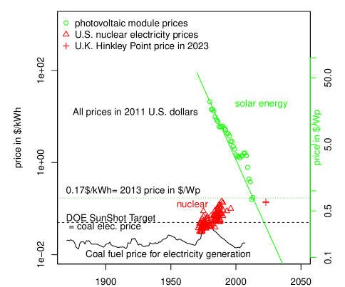
Figure 1: A comparison of long-term price trends for coal, nuclear power and solar photovoltaic modules. Prices for coal and nuclear power are costs in the US in dollars per kilowatt hour (scale on the left) whereas solar modules are in dollars per watt-peak, i.e. the cost for the capacity to generate a watt of electricity in full sunlight (scale on the right). For coal we use units of the cost of the coal that would need to be burned in a modern US plant if it were necessary to buy the coal at its inflation-adjusted price at different points in the past. Nuclear prices are Busbar costs for US nuclear plants in the year in which they became operational (from Cooper (2009)). The alignment of the left and right vertical axes is purely suggestive; based on recent estimates of levelized costs, we took $\$0.177/\mbox{kWh}=\$0.82/\mbox{Wp}$ in 2013 (2013$). The number $0.177/kWh is a global value produced as a projection for 2013 by the International Energy Agency (Table 4 in International Energy Agency (2014)). We note that it is compatible with estimated values (Table 1 in Baker et al. (2013), Fig. 4 in International Energy Agency (2014)). The red cross is the agreed price for the planned UK Nuclear power plant at Hinkley Point which is scheduled to come online in 2023 (£0.0925 $\approx$ $0.14). The dashed line corresponds to an earlier target of $\$0.05/\mbox{kWh}$ set by the the U.S. Department of Energy.

In this paper we use a very simple approach to forecasting that was originally motivated by Moore’s Law. As everyone knows, Intel’s ex-CEO, Gordon Moore, famously predicted that the number of transistors on integrated circuits would double every two years, i.e. at an annual rate of about 40%. Making transistors smaller also brings along a variety of other benefits, such as increased speed, decreased power consumption, and less expensive manufacture costs per unit of computation. As a result it quickly became clear that Moore’s law applies more broadly, for example, implying a doubling of computational speed every 18 months.

Moore’s law stimulated others to look at related data more carefully, and they discovered that exponential improvement is a reasonable approximation for other types of computer hardware as well, such as hard drives. Since the performance of hard drives depends on physical factors that are unrelated to transistor density this is an independent fact, though of course the fact that mass storage is essential for computation causes a tight coupling between the two technologies. Lienhard, Koh and Magee, and others examined data for other products, including many that have nothing to do with computation or information processing, and postulated that exponential improvement is a much more general phenomenon that applies to many different technologies, even if in most cases the exponential rates are much slower.

Although Moore’s law is traditionally applied as a regression of the log of the cost on a deterministic time trend, we reformulate it here as a geometric random walk with drift. This has several advantages. On average it results in more accurate forecasts, especially at short horizons, indicating that it is indeed a better model. In addition, this allows us to use standard results from the time series forecasting literature. The technology time series in our sample are typically rather short, often only 15 or 20 points long, so to test hypotheses it is essential to pool the data. Because the geometric random walk is so simple it is possible to derive formulas for the forecast errors in closed form. This makes it possible to estimate the forecast errors as a function of both sample size and forecasting horizon, and to combine data from many different technologies into a single analysis. This allows us to get highly statistically significant results. And most importantly, because this allows us to systematically test the method on data for many different technologies, this allows us to make distributional forecasts for a single technology and have confidence in the results.

Motivated by structure we find in the data, we further extend Moore’s law to allow for the possibility that changes in price are positively autocorrelated in time. We assume that the logarithm of the cost follows a random walk with drift and autocorrelated noise, more specifically an Integrated Moving Average process of order (1,1), i.e. an IMA(1,1) model. Under the assumption of sufficiently large autocorrelation this method produces a good fit to the empirically observed forecasting errors. We derive a formula for the errors of this more general model, assuming that all technologies have the same autocorrelation parameter and the forecasts are made using the simple random walk model. We use this to forecast the likely distribution of the price of photovoltaic solar modules, and to estimate the probability that solar modules will undercut a competing technology at a given date in the future.

We want to stress that we do not mean to claim that the generalizations of Moore’s law explored here provide the most accurate possible forecasts for technological progress. There is a large literature on experience curves, studying the relationship between cost and cumulative production originally suggested by Wright (1936), and many authors have proposed alternatives and generalizations. Nagy et al. (2013) tested these alternatives using a data set that is very close to ours and found that Moore’s and Wright’s laws were roughly tied for first place in terms of their forecasting performance. An important caveat is that Nagy et al.’s study was based on a trend stationary model, and as we argue here, the difference stationary model is superior, both for forecasting and for statistical testing. It seems likely that methods using auxiliary data such as production, patent activity, or R&D can be used to make forecasts for technological progress that incorporate more factors, and that such methods should yield improvements over the simple method we use here.

The key assumption made here is that all technologies follow the same random process, even if the drift and volatility parameters of the random process are technology specific. This allows us to develop distributional forecasts in a highly parsimonious manner and efficiently test them out of sample. We restrict ourselves to forecasting unit cost in this paper, for the simple reason that we have data for it and it is comparable across different technologies. The work presented here provides a simple benchmark against which to compare forecasts of future technological performance based on other methods.

The approach of basing technological forecasts on historical data that we pursue here stands in sharp contrast to the most widely used method, which is based on expert opinions. The use of expert opinions is clearly valuable, and we do not suggest that it should be supplanted, but it has several serious drawbacks. Expert opinions are subjective and can be biased for a variety of reasons (Albright, 2002), including common information, herding, or vested interest. Forecasts for the costs of nuclear power in the US, for example, were for several decades consistently low by roughly a factor of three (Cooper, 2009). A second problem is that it is very hard to assess the accuracy of expert forecasts. In contrast the method we develop here is objective and the quality of the forecasts is known. Nonetheless we believe that both methods are valuable and that they should be used side-by-side.

The remainder of the paper develops as follows: In Section 2 we derive the error distribution for forecasts based on the geometric random walk as a function of time horizon and other parameters and show how the data for different technologies and time horizons should be collapsed. We also show how this can be generalized to allow for autocorrelations in the data and derive similar (approximate) formulas. In Section 3 we describe our data set and present an empirical relationship between the variance of the noise and the improvement rate for different technologies. In Section 4 we describe our method of testing the models against the data, and present the results in Section 5. We then apply our method to give a distributional forecast for solar module prices in Section 6 and show how this can be used to forecast the likelihood that one technology will overtake another. Finally we give some concluding remarks in Section 7. A variety of technical results are given in the appendices.

2 Models

2.1 Geometric random walk

In this section we discuss how to formulate Moore’s law in the presence of noise and argue that the best method is the geometric random walk with drift. We then present a formula for the distribution of expected errors as a function of the time horizon and the other parameters of the model, and generalize the formula to allow for autocorrelation in the data generating process. This allows us to pool the errors for many different technologies. This is extremely useful because it makes it possible to test the validity of these results using many short time series (such as the data we have here).

The generalized version of Moore’s law we study here is a postulated relationship which in its deterministic form is

$$p_{t}=p_{0}e^{\mu t},$$

where $p_{t}$ is either the unit cost or the unit price of a technology at time $t$; we will hereafter refer to it as the cost. $p_{0}$ is the initial cost and $\mu$ is the exponential rate of change. (If the technology is improving then $\mu<0$.) In order to fit this to data one has to allow for the possibility of errors and make an assumption about the structure of the errors. Typically the literature has treated Moore’s law using a trend stationary model, minimizing squared errors to fit a model of the form

$$y_{t}=y_{0}+\mu t+e_{t},$$ (1)

where $y_{t}=\log(p_{t})$. From the point of view of the regression, $y_{0}$ is the intercept, $\mu$ is the slope and $e_{t}$ is independent and identically distributed (IID) noise.

But records of technological performance such as those we study here are time series, giving the costs $p_{jt}$ for technology $j$ at successive times $t=1,2,\ldots,T_{j}$. It is therefore more natural to use a time series model. The simplest possible choice that yields Moore’s law in the deterministic limit is the geometric random walk with drift,

$$y_{t}=y_{t-1}+\mu+n_{t}.$$ (2)

As before $\mu$ is the drift and $n_{t}$ is an IID noise process. Letting the noise go to zero recovers the deterministic version of Moore’s law in either case. When the noise is nonzero, however, the models behave quite differently. For the trend stationary model the shocks are purely transitory, i.e. they do not accumulate. In contrast, if $y_{0}$ is the cost at time $t=0$, Eq. (2) can be iterated and written in the form

$$y_{t}=y_{0}+\mu t+\sum_{i=1}^{t}n_{i}.$$ (3)

This is equivalent to Eq. (1) except for the last term. While in the regression model of Eq. (1) the value of $y_{t}$ depends only on the current noise and the slope $\mu$, in the random walk model (Eq. 2) it depends on the sum of previous shocks. Hence shocks in the random walk model accumulate and the forecasting errors grow with time horizon as one would expect, even if the parameters of the model are perfectly estimated..

For time series models a key question is whether the process has a unit root. Most of our time series are much too short for unit root tests to be effective (Blough, 1992). Nonetheless, we found that our time series forecasts are consistent with the hypothesis of a unit root and that they perform better than several alternatives.

2.2 Prediction of forecast errors

We now derive a formula for the forecast errors of the geometric random walk as a function of time horizon. We assume that all technologies follow the geometric random walk, i.e. our noisy version of Moore’s law, but with technology-specific parameters. Rewriting Eq. (2) slightly, it becomes

$$y_{jt}=y_{j,(t-1)}+\mu_{j}+n_{jt},$$

where the index $j$ indicates technology $j$. For convenience we assume that noise $n_{jt}$ is IID normal, i.e. $n_{jt}\sim\mathcal{N}(0,K_{j}^{2})$. This means that technology $j$ is characterized by a drift $\mu_{j}$ and the standard deviation of the noise increments $K_{j}$. We will typically not include the indices for the technology unless we want to emphasize the dependence on the technology.

We now derive the expected error distribution for Eq. (2) as a function of the time horizon $\tau$. Eq. (2) implies that

$$y_{t+\tau}=y_{t}+\mu\tau+\sum_{i=t+1}^{t+\tau}n_{i}.$$ (4)

The point forecast $\tau$ steps ahead is

$$\hat{y}_{t+\tau}=y_{t}+\hat{\mu}\tau,$$ (5)

where $\hat{\mu}$ is the estimated $\mu$. The forecast error is defined as

$$\mathcal{E}=y_{t+\tau}-\hat{y}_{t+\tau}.$$ (6)

Putting Eqs. (4) and (5) into Eq. (6) gives

$$\mathcal{E}=\tau(\mu-\hat{\mu})+\sum_{i=t+1}^{t+\tau}n_{i},$$ (7)

which separates the error into two parts. The first term is the error due to the fact that the mean is an estimated parameter and the second term represents the error due to the fact that unpredictable random shocks accumulate (Sampson, 1991). Assuming that the noise increments are i.i.d normal and that the estimation of the parameters is based on a trailing sample of $m$ data points, in Appendix B.1 we derive the scaling of the errors with $m$, $\tau$ and $\hat{K}$, where $\hat{K}^{2}$ is the estimated variance.

Because we want to aggregate forecast errors for technologies with different volatilities, to study how the errors grow as a function of $\tau$ we use the normalized mean squared forecast error $\Xi(\tau)$. Assuming $m>3$ it is

$$\Xi(\tau)\equiv E\left[\left(\frac{\mathcal{E}}{\hat{K}}\right)^{2}\right]=\frac{m-1}{m-3}\hskip 2.84526pt\left(\tau+\frac{\tau^{2}}{m}\right),$$ (8)

where $E$ represents the expectation.

This formula makes intuitive sense. The diffusion term $\tau$ is due to the accumulation of noisy fluctuations through time. This term is present even in the limit $m\to\infty$, where the estimation is perfect. The $\tau^{2}/m$ term is due to estimation error in the mean. The need to estimate the variance causes the prefactor $(m-1)/(m-3)$ and also means that the distribution is Student $t$ rather than normal, i.e.

$$\epsilon=\frac{1}{\sqrt{A}}\left(\frac{\mathcal{E}}{\hat{K}}\right)\sim t(m-1),$$ (9)

with

$$A=\tau+\tau^{2}/m.$$ (10)

Eq. (9) is universal in the sense that the right hand side is independent of $\hat{\mu}_{j}$, $\hat{K}_{j}$, and $\tau$. It depends neither on the properties of the technology nor on the time horizon. As a result we can pool forecast errors for different technologies at different time horizons. This property is extremely useful for statistical testing and can also be used to construct distributional forecasts for a given technology.

2.3 Generalization for autocorrelation

We now generalize the formula above to allow for autocorrelations in the error terms. Although the uncorrelated random walk model above does surprisingly well, there is good evidence that there are positive autocorrelations in the data. In order to incorporate this structure we extend the results above for an ARIMA(0,1,1) (autoregressive integrated moving average) model. The zero indicates that we do not use the autoregressive part, so we will abbreviate this as an IMA(1,1) model in what follows. The IMA(1,1) model is of the form

$$y_{t}-y_{t-1}=\mu+v_{t}+\theta v_{t-1},$$ (11)

with the noise $v_{t}\sim\mathcal{N}(0,\sigma^{2})$. This model is also a geometric random walk, but with correlated increments when $\theta\neq 0$ (the autocorrelations of the time series are positive when $\theta>0$).

We chose this model rather than other alternatives mainly for its simplicity. Moreover, our data are often time-aggregated, that is, our yearly observations are averages of the observed costs over the year. It has been shown that if the true process is a random walk with drift then aggregation can lead to substantial autocorrelation (Working, 1960). In any case, while every technology certainly follows an idiosyncratic pattern and may have a complex autocorrelation structure and specific measurement errors, using the IMA(1,1) as a universal model allows us to parsimoniously understand the empirical forecast errors and generate robust prediction intervals.

A key quantity for pooling the data is the variance, which by analogy with the previous model we call $K$ for this model as well. It is easy to show that

$$K^{2}\equiv var(y_{t}-y_{t-1})=var(v_{t}+\theta v_{t-1})=(1+\theta^{2})\sigma^{2},$$

see e.g. Box & Jenkins (1970). The relevant formulas for this case are derived in Appendix B.2. We make the same point forecasts as before given by Eq. (5). If the variance is known the distribution of forecast errors is

$$\mathcal{E}\sim\mathcal{N}(0,\sigma^{2}A^{*}),$$ (12)

with

$$A^{*}=-2\theta+\left(1+\frac{2(m-1)\theta}{m}+\theta^{2}\right)\left(\tau+\frac{\tau^{2}}{m}\right).$$ (13)

Note that we recover Eq. (10) when $\theta=0$. In the usual case where the variance has to be estimated, we derive an approximate formula for the growth and distribution of the forecast errors by assuming that $\hat{K}$ and $\mathcal{E}$ are independent. The expected mean squared normalized error is

$$\Xi(\tau)\equiv E\left[\left(\frac{\mathcal{E}}{\hat{K}}\right)^{2}\right]=\frac{m-1}{m-3}\hskip 2.84526pt\frac{A^{*}}{1+\theta^{2}},$$ (14)

and the distribution of rescaled normalized forecast errors is

$$\epsilon^{*}=\frac{1}{\sqrt{A^{*}/(1+\theta^{2})}}\left(\frac{\mathcal{E}}{\hat{K}}\right)\sim t(m-1).$$ (15)

These formulas are only approximations so we compare them to more exact results obtained through simulations in Appendix B.2 – see in particular Fig. 12. For $m>30$ the approximation is excellent, but there are discrepancies for small values of $m$.

As before the right hand side is independent of all the parameters of the technology as well as the time horizon. Eq. (15) can be viewed as the distribution of errors around a point forecast, which makes it possible to collapse many technologies onto a single distribution. This property is extremely useful for statistical testing, i.e. for determining the quality of the model. But its greatest use, as we demonstrate in Section 6, is that it makes it possible to formulate a distributional forecast for the future costs of a given technology.

When $m$ is sufficiently large the Student $t$ distribution is well-approximated by a standard normal. Using the mean given by Eq. (5) and the variance determined by Eqs. (12-13), the distributional forecast for the future logarithm of the cost $y_{t+\tau}$ conditioned on $(y_{t},\ldots,y_{t-m+1})$ is

$$y_{t+\tau}\sim\mathcal{N}(y_{t}+\hat{\mu}\tau,\hat{K}^{2}A^{*}/(1+\theta^{2})).$$ (16)

We will return later to the estimation of $\theta$.

2.4 Alternative hypotheses

In addition to autocorrelation we investigated other ways to generalize the model, such as heavy tails and long-memory. As discussed in Appendix C.4, based on forecast errors we found little evidence for heavy tails. Long-memory is in a sense an extreme version of the autocorrelation hypothesis, which produces errors that grow faster as a function of the forecasting horizon $\tau$ than a random walk. Given that long-memory is a natural result of nonstationarity, which is commonly associated with technological change, our prior was that it was a highly plausible alternative. However, as we will see, the geometric random walk with normal noise increments and autocorrelations seems to give good agreement for the time scaling of forecasting errors, so we did not investigate long-memory further.

3 Data

3.1 Data collection

The bulk of our data on technology costs comes from the Santa Fe Institute’s Performance Curve DataBase, which was originally developed by Bela Nagy and collaborators; we augment it with a few other datasets. These data were collected via literature search, with the principal criterion for selection being availability. Fig. 2 plots the time series for each data set. The motley character of our dataset is clear: The time series for different technologies are of different lengths and they start and stop at different times. The sharp cutoff for the chemical data, for example, reflects the fact that it comes from a book published by the Boston Consulting Group in 1972. Table 1 gives a summary of the properties of the data and more description of the sources can be found in Appendix A. This plot also makes it clear that technologies improve at very different rates.

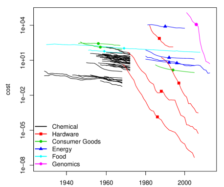
Figure 2: Cost vs. time for each technology in our dataset. This shows the 53 technologies out of the original set of 66 that have a significant rate of cost improvement (DNA sequencing is divided by 1000 to fit on the plot; the $y$-axis is in log scale). More details can be found in Table 1 and Appendix A.

A ubiquitous problem in forecasting technological progress is finding invariant units. A favorable example is electricity. The cost of generating electricity can be measured in dollars per kWh, making it possible to sensibly compare competing technologies and measure their progress through time. Even in this favorable example, however, making electricity cleaner and safer has a cost, which has affected historical prices for technologies such as coal and nuclear power in recent years, and means that their costs are difficult to compare to clean and safe but intermittent sources of power such as solar energy. To take an unfavorable example, our dataset contains appliances such as television sets, that have dramatically increased in quality through time. Yet another problem is that some of them are potentially subject to scarcity constraints, which might potentially introduce additional trends and fluctuations.

One should therefore regard our results here as a lower bound on what is possible, in the sense that performing the analysis with better data in which all technologies had invariant units would very likely improve the quality of the forecasts. We would love to be able to make appropriate normalizations but the work involved is prohibitive; if we dropped all questionable examples we would end with little remaining data. Most of the data are costs, but in a few cases they are prices; again, this adds noise but if we were able to be consistent that should only improve our results. We have done various tests removing data and the basic results are not sensitive to what is included and what is omitted (see Fig. 14 in the appendix).

We have removed some technologies that are too similar to each other from the Performance Curve Database. For instance, when we have two datasets for the same technology, we keep only one of them. Our choice was based on data quality and length of the time series. This selection left us with 66 technologies belonging to different sectors that we label as chemistry, genomics, energy, hardware, consumer durables and food.

3.2 Data selection and descriptive statistics

In this paper we are interested in technologies that are improving, so we restrict our analysis to those technologies whose rate of improvement is statistically significant based on the available sample. We used a simple one-sided $t$-test on the first-difference (log) series and removed all technologies for which the $p$-value indicates that we can’t reject the null that $\mu_{j}=0$ at a 10% confidence level.

Technology	Industry	T	$\tilde{\mu}$	$p$ value	$\tilde{K}$	$\tilde{\theta}$
Transistor	Hardware	38	-0.50	0.00	0.24	0.19
Geothermal.Electricity	Energy	26	-0.05	0.00	0.02	0.15
Milk..US.	Food	79	-0.02	0.00	0.02	0.04
DRAM	Hardware	37	-0.45	0.00	0.38	0.14
Hard.Disk.Drive	Hardware	20	-0.58	0.00	0.32	-0.15
Automotive..US.	Cons. Goods	21	-0.08	0.00	0.05	1.00
Low.Density.Polyethylene	Chemical	17	-0.10	0.00	0.06	0.46
Polyvinylchloride	Chemical	23	-0.07	0.00	0.06	0.32
Ethanolamine	Chemical	18	-0.06	0.00	0.04	0.36
Concentrating.Solar	Energy	26	-0.07	0.00	0.07	0.91
AcrylicFiber	Chemical	13	-0.10	0.00	0.06	0.02
Styrene	Chemical	15	-0.07	0.00	0.05	0.74
Titanium.Sponge	Chemical	19	-0.10	0.00	0.10	0.61
VinylChloride	Chemical	11	-0.08	0.00	0.05	-0.22
Photovoltaics	Energy	34	-0.10	0.00	0.15	0.05
PolyethyleneHD	Chemical	15	-0.09	0.00	0.08	0.12
VinylAcetate	Chemical	13	-0.08	0.00	0.06	0.33
Cyclohexane	Chemical	17	-0.05	0.00	0.05	0.38
BisphenolA	Chemical	14	-0.06	0.00	0.05	-0.03
Monochrome.Television	Cons. Goods	22	-0.07	0.00	0.08	0.02
PolyethyleneLD	Chemical	15	-0.08	0.00	0.08	0.88
Laser.Diode	Hardware	13	-0.36	0.00	0.29	0.37
PolyesterFiber	Chemical	13	-0.12	0.00	0.10	-0.16
Caprolactam	Chemical	11	-0.10	0.00	0.08	0.40
IsopropylAlcohol	Chemical	9	-0.04	0.00	0.02	-0.24
Polystyrene	Chemical	26	-0.06	0.00	0.09	-0.04
Polypropylene	Chemical	10	-0.10	0.00	0.07	0.26
Pentaerythritol	Chemical	21	-0.05	0.00	0.07	0.30
Ethylene	Chemical	13	-0.06	0.00	0.06	-0.26
Wind.Turbine..Denmark.	Energy	20	-0.04	0.00	0.05	0.75
Paraxylene	Chemical	12	-0.10	0.00	0.09	-1.00
DNA.Sequencing	Genomics	13	-0.84	0.00	0.83	0.26
NeopreneRubber	Chemical	13	-0.02	0.00	0.02	0.83
Formaldehyde	Chemical	11	-0.07	0.00	0.06	0.36
SodiumChlorate	Chemical	15	-0.03	0.00	0.04	0.85
Phenol	Chemical	14	-0.08	0.00	0.09	-1.00
Acrylonitrile	Chemical	14	-0.08	0.01	0.11	1.00
Beer..Japan.	Food	18	-0.03	0.01	0.05	-1.00
Primary.Magnesium	Chemical	40	-0.04	0.01	0.09	0.24
Ammonia	Chemical	13	-0.07	0.02	0.10	1.00
Aniline	Chemical	12	-0.07	0.02	0.10	0.75
Benzene	Chemical	17	-0.05	0.02	0.09	-0.10
Sodium	Chemical	16	-0.01	0.02	0.02	0.42
Methanol	Chemical	16	-0.08	0.02	0.14	0.29
MaleicAnhydride	Chemical	14	-0.07	0.03	0.11	0.73
Urea	Chemical	12	-0.06	0.03	0.09	0.04
Electric.Range	Cons. Goods	22	-0.02	0.03	0.04	-0.14
PhthalicAnhydride	Chemical	18	-0.08	0.03	0.15	0.31
CarbonBlack	Chemical	9	-0.01	0.03	0.02	-1.00
Titanium.Dioxide	Chemical	9	-0.04	0.04	0.05	-0.41
Primary.Aluminum	Chemical	40	-0.02	0.06	0.08	0.39
Sorbitol	Chemical	8	-0.03	0.06	0.05	-1.00
Aluminum	Chemical	17	-0.02	0.09	0.04	0.73
Free.Standing.Gas.Range	Cons. Goods	22	-0.01	0.10	0.04	-0.30
CarbonDisulfide	Chemical	10	-0.03	0.12	0.06	-0.04
Ethanol..Brazil.	Energy	25	-0.05	0.13	0.22	-0.62
Refined.Cane.Sugar	Food	34	-0.01	0.23	0.06	-1.00
CCGT.Power	Energy	10	-0.04	0.25	0.15	-1.00
HydrofluoricAcid	Chemical	11	-0.01	0.25	0.04	0.13
SodiumHydrosulfite	Chemical	9	-0.01	0.29	0.07	-1.00
Corn..US.	Food	34	-0.02	0.30	0.17	-1.00
Onshore.Gas.Pipeline	Energy	14	-0.02	0.31	0.14	0.62
Motor.Gasoline	Energy	23	-0.00	0.47	0.05	0.43
Magnesium	Chemical	19	-0.00	0.47	0.04	0.58
Crude.Oil	Energy	23	0.01	0.66	0.07	0.63
Nuclear.Electricity	Energy	20	0.13	0.99	0.22	-0.13

Table 1: Descriptive statistics and parameter estimates (using the full sample) for all available technologies. They are ordered by the $p$-value of a one-sided $t$-test for $\tilde{\mu}$, i.e. based on how strong the evidence is that they are improving. The improvement of the last 13 technologies is not statistically significant and so they are dropped from further analysis – see the discussion in the text.

Table 1 reports the $p$-values for the one sided $t$-tests and the bottom of the table shows the technologies that are excluded as a result. Table 1 also shows the estimated drift $\tilde{\mu}_{j}$ and the estimated standard deviation $\tilde{K_{j}}$ based on the full sample for each technology $j$. (Throughout the paper we use a hat to denote estimates performed within an estimation window of size $m$ and a tilde to denote the estimates made using the full sample). Histograms of $\tilde{\mu}_{j}$, $\tilde{K}_{j}$, sample size $T_{j}$ and $\tilde{\theta}_{j}$ are given in Fig. 3.

Figure 3: Histogram for the estimated parameters for each technology $i$ based on the full sample (see also Table 1). $\tilde{\mu}_{j}$ is the annual logarithmic rate of decrease in cost, $\tilde{K}_{j}$ is the standard deviation of the noise, $T_{j}$ is the number of available years of data and $\tilde{\theta}_{j}$ is the autocorrelation.

3.3 Relation between drift and volatility

Fig. 4 shows a scatter plot of the estimated standard deviation $\tilde{K}_{j}$ for technology $j$ vs. the estimated improvement rate $-\tilde{\mu}_{j}$. A linear fit gives $\tilde{K}=0.02-0.76\tilde{\mu}$ with $R^{2}=0.87$ and standard errors of $0.008$ for the intercept and $0.04$ for the slope, as shown in the figure. A log-log fit gives $\tilde{K}=e^{-0.68}(-\tilde{\mu})^{0.72}$ with $R^{2}=0.73$ and standard errors for the scaling constant of $0.18$ and for the exponent of $0.06$. This indicates that on average the uncertainty $\tilde{K}_{j}$ gets bigger as the improvement rate $-\tilde{\mu_{j}}$ increases. There is no reason that we are aware of to expect this a priori. One possible interpretation is that for technological investment there is a trade-off between risk and returns. Another possibility is that faster improvement amplifies fluctuations.

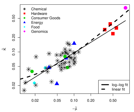
Figure 4: Scatter plot of the estimated standard deviation $\tilde{K_{j}}$ for technology $j$ against its estimated improvement rate $-\tilde{\mu}_{j}$. The dashed line shows a linear fit (which is curved when represented in log scale); the solid line is a log-log fit. Technologies with a faster rate of improvement have higher uncertainty in their improvement.

4 Estimation procedures

4.1 Statistical validation

We use hindcasting for statistical validation, i.e. for each technology we pretend to be at a given date in the past and make forecasts for dates in the future relative to the chosen date. We have chosen this procedure for several reasons. First, it directly tests the predictive power of the model rather than its goodness of fit to the data, and so is resistant to overfitting. Second, it mimics the same procedure that one would follow in making real predictions, and third, it makes efficient use of the data available for testing.

We fit the model at each time step to the $m$ most recent changes in cost (i.e. the most recent $m+1$ years of data). We use the same value of $m$ for all technologies and for all forecasts. Because most of the time series in our dataset are quite short, and because we are more concerned here with testing the procedure we have developed rather than with making optimal forecasts, unless otherwise noted we choose $m=5$. This is admittedly very small, but it has the advantage that it allows us to make a large number of forecasts. We will return later to discuss the question of which value of $m$ makes the best forecasts.

We perform hindcasting exhaustively in the sense that we make as many forecasts as possible given the choice of $m$. For technology $j$, the cost data $y_{t}=\log p_{t}$ exists in years $t=1,2,\ldots,T_{j}$. We then make forecasts for each feasible year and each feasible time horizon, i.e. we make forecasts $\hat{y}_{t_{0}+\tau}(t_{0})$ rooted in years $t_{0}=(m+1,\ldots,T_{j}-1)$ with forecast horizon $\tau=(1,\ldots,T_{j}-t_{0})$.

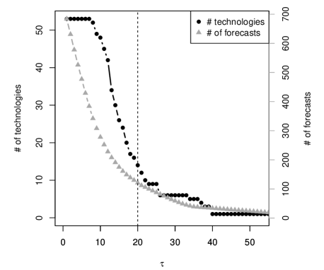
Figure 5: Data available for testing as a function of the forecast time horizon. Here # of technologies refers to the number of technology time series that are long enough to make at least one forecast at a given time horizon $\tau$, which is measured in years. Similarly # of forecasts refers to the total number of forecasts that can be made at time horizon $\tau$. The horizontal line at $\tau=20$ years indicates our (somewhat arbitrary) choice of a maximum time horizon.

Since our dataset includes technology time series of different length (see Table 1 and Fig. 2) the number of possible forecasts that can be made with a given historical window $m$ is highest for $\tau=1$ and decreases for longer horizons. Fig. 5 shows the total number of possible forecasts that can be made with our dataset at a given horizon $\tau$ and the number of technology time series that are long enough to make at least one forecast at horizon $\tau$. This shows that the amount of available data decreases dramatically for large forecast horizons. We somewhat arbitrarily impose an upper bound of $\tau_{max}=20$, but find this makes very little difference in the results (see Appendix C.3). There are a total of 8212 possible forecasts that can be made with an historical window of $m=5$, and 6391 forecasts that can be made with $\tau\leq 20$.

To test for statistical significance we use a surrogate data procedure (explained below). There are three reasons for doing this: The first is that, although we derived approximate formulas for the forecast errors in Eq. (14) and (15), when $\theta\neq 0$ the approximation is not very good for $m=5$. The second is that the rolling window approach we use for hindcasting implies overlaps in both the historical sample used to estimate parameters at each time $t_{0}$ and overlapping intervals in the future for horizons with $\tau>1$. This implies substantial correlation in the empirical forecast errors, which complicates statistical testing. The third reason is that, even if the formulas were exact, we expect finite sample fluctuations. That is, with a limited number of technologies and short time series, we do not expect to find the predicted result exactly; the question is then whether the deviation that we observe is consistent with what is expected.

The surrogate data procedure estimates a null distribution for the normalized mean squared forecast error under the hypothesized model. This is done by simulating both the model and the forecasting procedure to create a replica of the dataset and the forecasts. This is repeated for many different realizations of the noise process in order to generate the null distribution. More specifically, for each technology we generate $T_{j}$ pseudo cost data points using Eq. (11) with $\mu=\tilde{\mu}_{j}$, $K=\tilde{K}_{j}$ and a given value of $\theta$, thereby mimicking the structure of the data set. We then estimate the parameters and perform hindcasting just as we did for the real data, generating the same number of forecasts and computing the mean squared forecast error. This process is then repeated many times with different random number seeds to estimate the distribution. This same method can be used to estimate expected deviations for any quantity, e.g. we also use this to estimate the expected deviation of the finite sample distribution from the predicted distribution of forecast errors.

4.2 Parameter estimation

We estimate the mean and the variance for each technology dynamically, using a rolling window approach to fit the parameters based on the $m+1$ most recent data points. In each year $t_{0}$ for which forecasts are made the drift $\hat{\mu}_{t_{0}}$ is estimated as the sample mean of the first differences,

$$\hat{\mu}_{t_{0}}=\frac{1}{m}\sum_{i=t_{0}-m}^{t_{0}-1}(y_{i+1}-y_{i})=\frac{y_{t_{0}}-y_{t_{0}-m}}{m},$$ (17)

where the last equality follows from the fact that the sum is telescopic, and implies that only two points are needed to estimate the drift. The volatility is estimated using the unbiased estimator

$$\hat{K}^{2}_{t_{0}}=\frac{1}{m-1}\sum_{i=t_{0}-m}^{t_{0}-1}[(y_{i+1}-y_{i})-\hat{\mu}_{t_{0}}]^{2}.$$ (18)

This procedure gives us a variable number of forecasts for each technology $j$ and time horizon $\tau$ rooted at all feasible times $t_{0}$. We record the forecasting errors $\mathcal{E}_{t_{0},\tau}=y_{t+\tau}(t_{0})-\hat{y}_{t+\tau}(t_{0})$ and the associated values of $\hat{K}_{t_{0}}$ for all $t_{0}$ and all $\tau$ where we can make forecasts.

The autocorrelation parameter $\theta$ for the generalized model has to be treated differently. Our time series are simply too short to make reasonable rolling window, technology-specific estimates for $\theta$. With such small values of $m$ the estimated autocorrelations are highly unreliable.

Our solution is to use a global value of $\theta$, i.e. we use the same value for all technologies and all points in time. It may well be that $\theta$ is technology specific, but given the short amount of data it is necessary to make a choice that performs well under forecasting. This is a classic bias-variance trade-off, where the variance introduced by statistical estimation of a parameter is so large that the forecasts produced by a biased model with this parameter fixed are superior. With very long time series this could potentially be avoided. This procedure seems to work well. It leaves us with a parameter that has to be estimated in-sample, but since this is only one parameter estimated from a sample of more than $6,000$ forecasts the resulting estimate should be reasonably reliable.

Evidence concerning autocorrelations is given in Fig. 3, where we present a histogram for the values of $\tilde{\theta}_{j}$ for each technology $j$ based on the full sample. The results are highly variable. Excluding eight likely outliers where $\tilde{\theta}_{j}=\pm 1$, the mean across the sample is $0.27$, and 35 out of the remaining 45 improving technologies have positive values of $\tilde{\theta}_{j}$. This seems to suggest that $\theta$ tends to be positive.

We use two different methods for estimating a global value of $\theta$. The first method takes advantage of the fact that the magnitude of the forecast errors is an increasing function of $\theta$ (we assume $\theta>0$) and chooses $\theta_{m}$ ($m$ as in “matched”) to match the empirically observed forecast errors, leading to $\theta_{m}=0.63$ as described in the next section. The second method takes a weighted average $\theta_{w}$ ($w$ as in “weighted”) calculated as follows. We exclude all technologies for which the estimate of $\theta$ reveals specification or estimation issues ($\theta\approx 1$ or $\theta\approx-1$). Then at each horizon we compute a weighted average, with the weights proportional to the number of forecasts made with that technology. Finally we take the average of the first 20 horizon-specific estimated values of $\theta$, leading to $\theta_{w}=0.25$. See Appendix D.

5 Comparison of models to data

In comparing the model to data we address the following five questions:

1. Is the scaling law for the increase in forecasting errors as a function of time derived in Eqs. (8) and (14) consistent with the data?

2. Does there exist a value of $\theta$ such that the null hypothesis of the model is not rejected? If so, what is this value, and how strong is the evidence that it is positive?

3. When the normalized errors for different technologies at different time horizons are collapsed onto a single distribution, does this agree with the Student distribution as predicted by Eq. (15)?

4. Do the errors scale with the trailing sample size $m$ as predicted under the assumption that the random process is stationary (i.e. that parameters are not changing in time)?

5. Is the model well-specified?

We will see that we get clear affirmative answers to the first four questions but we are unable to answer question (5).

5.1 Normalized forecast errors as a function of $\tau$

To answer the first question we compute the sample estimate of the mean squared normalized forecast error $\Xi(\tau)$, averaging over all available forecasts for all technologies at each time horizon with $\tau\leq 20$ (see Eq. (14)). Fig. 6 compares the empirical results to the model with three different values of the autocorrelation parameter $\theta$. Because the approximate error estimates derived in Eq. (14) break down for small values of $m$, for each value of $\theta$ we estimate the expected mean squared errors under the null hypothesis of the model via the surrogate data procedure described in Section 4.1.

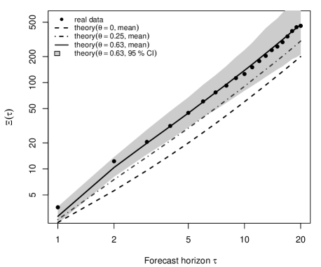
Figure 6: Growth of the mean squared normalized forecast error $\Xi(\tau)$ for the empirical forecasts compared to predictions using different values of $\theta$. The empirical value of the normalised error $\Xi(\tau)$ is shown by black dots. The grey area corresponds to the $95\%$ confidence intervals for the case $\theta=\theta_{m}$. The dashed line represents the predicted squared normalized error with $\theta=0$, the dot-dash line is for $\theta_{w}=0.25$ and the solid line is for $\theta_{m}=0.63$.

The model does a good job of predicting the scaling of the forecast errors as a function of the time horizon $\tau$. The errors are predicted to grow approximately proportional to $(\tau+\tau^{2}/m)$; at long horizons the error growth at each value of $\theta$ closely parallels that for the empirical forecasts. This suggests that this scaling is correct, and that there is no strong support for modifications such as long-memory that would predict alternative rates of error growth.

Using $\theta_{m}=0.63$ gives a good match to the empirical data across the entire range of time horizons. Note that even though we chose $\theta_{m}$ in order to get the best possible match, given that we are rescaling data for different technologies by the empirically measured sample standard deviations over very short samples of length $m=5$, and that we are predicting across 20 different time horizons simultaneously, the ability to find a value of the parameter $\theta$ that matches this well was far from guaranteed. (It is completely possible, for example, that there would simply not exist a value of $\theta<1$ yielding errors that were sufficiently large).

To test the statistical significance of the results for different values of $\theta$ and $\tau$ we use the surrogate data procedure described at the end of Section 4.1. For $\theta_{m}=0.63$ we indicate error bars by showing in grey the region containing the 95% of the simulated realizations with errors closest to the mean. For $\tau=1$ and $\tau=2$ the predicted errors are visibly below the empirical observations, but the difference is within the error bars (though on the edge of the error bars for $\tau=1$); the agreement is very good at all other values of $\tau$. The autocorrelation parameter $\theta_{w}=0.25$ is weakly rejected for $\tau$ between 1 and 6 and weakly accepted elsewhere, indicating that it is very roughly the lowest value of $\theta$ that is consistent with the data at the two standard deviation level. In contrast the case $\theta=0$, which gives normalized error predictions that are lower by about a factor of two, is clearly well outside of the error bars (note the logarithmic scale). This strongly indicates that a positive value of $\theta$ is required to match the observed errors, satisfying $\theta>\theta_{w}=0.25$.

5.2 Distribution of forecast errors

We now address question (3) by testing whether we correctly predict the distribution of forecast errors. Fig. 7 shows the distribution of rescaled forecast errors using $\theta_{m}=0.63$ with Eq. (15) to rescale the errors. Different values of $\tau$ are plotted separately, and each is compared to the predicted Student distribution. Overall, the fit is good but at longer horizons forecast errors tend to be positive, that is, realized technological progress is slightly slower than predicted. We have tested to see if this forecast bias is significant, and for $\tau\leq 11$ we cannot reject the null that there is no bias even at the $10\%$ level. At higher horizons there is evidence of forecast bias, but we have to remember that at these horizons we have much less data (and fewer technologies) available for testing.

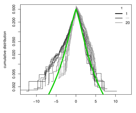
Figure 7: Cumulative distribution of empirical rescaled normalized forecast errors at different forecast horizons $\tau$. The forecast errors for each technology $j$ are collapsed using Eq. (15) with $\theta=\theta_{m}=0.63$. This is done for each forecast horizon $\tau=1,2,\ldots,20$ as indicated in the legend. The green thick curve is the theoretical prediction. The positive and negative errors are plotted separately. For the positive errors we compute the number of errors greater than a given value $X$ and divide by the total number of errors to estimate the cumulative probability and plot in semi-log scale. For the negative errors we do the same except that we take the absolute value of the error and plot against $-X$.

Fig. 8 shows the empirical distribution with all values of $\tau$ pooled together, using rescalings corresponding to $\theta=0$, $\theta_{w}$, and $\theta_{m}$. The predicted distribution is fairly close to the theoretical prediction, and as expected the fit with $\theta_{m}=0.63$ is better than with $\theta_{w}=0.25$ or $\theta=0$.

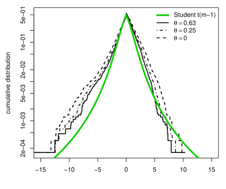
Figure 8: Cumulative distribution of empirical rescaled normalized forecast errors with all $\tau$ pooled together for three different values of the autocorrelation parameter, $\theta=0$ (dashed line), $\theta=0.25$ (dot-dash line) and $\theta=0.63$ (solid line). See the caption of Fig. 7 for a description of how the cumulative distributions are computed and plotted.

To test whether the observed deviations of the empirical error distribution from the predicted distribution are significant we once again use the surrogate data approach described at the end of Section 4.1. As before we generate many replicas of the dataset and forecasts. For each replica of the dataset and forecasts we compute a set of renormalized errors $\epsilon^{*}$ and construct their distribution. We then measure the average distance between the surrogate distribution and the Student distribution as described in Appendix E. Repeating this process 10,000 times results in the sampling distribution of the deviations from the Student distribution under the null hypothesis that the model is correct. We then compare this to the corresponding value of the average distance between the real data and the Student distribution, which gives us a $p$-value under the null hypothesis. We find that the model with $\theta_{m}=0.63$ is accepted. In contrast $\theta_{w}=0.25$ is rejected with $p$-values ranging from $1\%$ to $0.1\%$, depending on the way in which the average distance is computed. The case with $\theta=0$ is very strongly rejected.

These results make it clear that the positive autocorrelations are both statistically significant and important. The statistical testing shows that $\theta=0.63$ provides a good estimate for the observed forecasting errors across a large range of time horizons, with normalized forecasting errors that are well-described by the Student distribution.

5.3 Dependence on sample size $m$

So far we have used only a small fraction of the data to make each forecast. The choice for the trailing sample of $m=5$ was for testing purposes, allowing us to generate a large number of forecasts and test our method for estimating their accuracy.

We now address the question of the optimal value of $m$. If the process is stationary in the sense that the parameters $(\mu,K,\theta)$ are constant, one should always use the largest possible value of $m$. If the process is nonstationary, however, it can be advantageous to use a smaller value of $m$, or alternatively a weighted average that decays as it goes into the past. How stationary is the process generating technology costs, and what is the best choice of $m$?

We experimented with increasing $m$, as shown in Fig. 9, and compared this to the model with $\theta_{m}=0.63$. We find that the errors drop as $m$ increases roughly as one would expect if the process were stationary and that the model does a reasonably good job of forecasting the errors (see also Appendix C.1). This indicates that the best choice is the largest possible value of $m$, which in this case is $m=16$. However we should emphasize that it is entirely possible that testing on a sample with longer time series might yield an optimal value of $m>16$.

Figure 9: Mean squared normalized forecast error $\Xi$ as a function of the forecast horizon $\tau$ for different sizes of the trailing sample size $m$. This is done for $m=(4,8,12,16)$, as shown in the legend. The corresponding theoretical predictions are made using $\theta_{m}=0.63$, and are shown as solid curves ordered in the obvious way from top ($m=4$) to bottom ($m=16$).

5.4 Is the model well-specified?

Because most of our time series are so short it is difficult to say whether or not the model is well-specified. As already noted, for such short series it is impossible to usefully estimate technology-specific values of the parameter $\theta$, which has forced us to use a global value for all technologies. Averaging over the raw samples suggests a relatively low value $\theta_{w}=0.25$, but a much higher value $\theta_{m}=0.63$ is needed to match the empirically observed errors. However we should emphasize that with such short series $\theta$ is poorly estimated, and it is not clear that averaging across different technologies is sufficient to fix this problem.

In our view it would be surprising if there are not technology-specific variations in $\theta$; after all $\mu_{j}$ and $K_{j}$ vary significantly across technologies. So from this point of view it seems likely that the model with a global $\theta$ is mis-specified. It is not clear whether this would be true if we were able to measure technology-specific values of $\theta_{j}$. It is remarkable that such a simple model can represent a complicated process such as technological improvement as well as it does, and in any case, as we have shown, using $\theta=\theta_{m}$ does a good job of matching the empirically observed forecasting errors. Nonetheless, testing with more data is clearly desirable.

6 Application to solar PV modules

In this section we provide a distributional forecast for the price of solar photovoltaic modules. We then show how this can be used to make a comparison to a hypothetical competing technology in order to estimate the probability that one technology will be less expensive than another at a given time horizon.

6.1 A distributional forecast for solar energy

We have shown that the autocorrelated geometric random walk can be used to forecast technological cost improvement and that the formula we have derived for the distribution of forecast errors works well when applied to many different technologies. We now demonstrate how this can be used to make a distributional forecast for the cost improvement of a given technology. The fact that the method has been extensively tested on many technologies in the previous section gives us some confidence that this forecast is reliable.

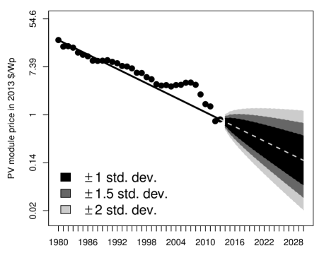
Figure 10: Forecast for the cost of photovoltaic modules in 2013 $/Wp. The point forecasts and the error bars are produced using Eq. (19) and the parameters discussed in the text. Shading indicates the quantiles of the distribution corresponding to 1, 1.5 and 2 standard deviations.

We make the forecast using Eq. (16). We use all available years of past data ($m=33$) to fit the parameters $\hat{\mu}_{S}=\tilde{\mu}_{S}=-0.10$ and $\hat{K}_{S}=\tilde{K}_{S}=0.15$, and we used $\theta=\theta_{m}=0.63$. The forecast is given by Eq. (16) with appropriate substitutions of parameters, i.e.

$$y_{S}(t+\tau)\sim\mathcal{N}(y_{S}(t)+\tilde{\mu}_{S}\tau,\tilde{K}_{S}^{2}A^{*}/(1+{\theta_{m}}^{2})),$$ (19)

where $A^{*}(\theta_{m})$ is defined in Eq. (13). Fig. 10 shows the predicted distribution of likely prices for solar photovoltaic modules for time horizons up to 2030. The intervals corresponding to plus or minus two standard deviations in Fig. 10 are 95% prediction intervals.

The prediction says that it is likely that solar PV modules will continue to drop in cost at the roughly $10\%$ rate that they have in the past. Nonetheless there is a small probability (about $5\%$) that the price in 2030 will be higher than it was in 2013 . While it might seem remarkable to forecast 15 years ahead with only 33 years of past data, note that throughout most of the paper we were forecasting up to 20 years ahead with only six years of data. As one uses more past data, the width of the distributional forecast decreases. In addition there are considerable variations in the standard deviations $\tilde{K}_{j}$ of the technologies in Table 1; these variations are reflected in the width of the distribution at any given forecasting horizon. The large deviation from the trend line that solar module costs made in the early part of the millennium cause the estimated future variance to be fairly large.

Except for the estimation of $\theta$ no data from other technologies was used in this forecast. Nonetheless, data from other technologies were key in giving us confidence that the distributional forecast is reliable.

6.2 Estimating the probability that one technology will be less expensive than another

Suppose we want to compute the probability that a given technology will be less expensive than another competing technology at a given point in the future. We illustrate how this can be done by comparing the log cost of photovoltaic modules $y_{S}$ with the log cost of a hypothetical alternative technology $y_{C}$. Both the cost of photovoltaic modules and technology C are assumed to follow Eq. (19), but for the sake of argument we assume that, like coal, technology $C$ has historically on average had a constant cost, i.e. $\tilde{\mu}_{C}=0$. We also assume that the estimation period is the same, and that $\theta_{C}=\theta_{S}=\theta_{m}$. We want to compute the probability that $\tau$ steps ahead $y_{S}<y_{C}$. The probability that $y_{S}<y_{C}$ is the probability that the random variable $Z=y_{C}-y_{S}$ is positive. Since $y_{S}$ and $y_{C}$ are normal, assuming they are independent their difference is normal, i.e.

$$Z\sim\mathcal{N}\left(\mu_{Z},\sigma_{Z}^{2}\right),$$

where $\mu_{Z}=(y_{C}(t)-y_{S}(t))+\tau(\tilde{\mu}_{C}-\tilde{\mu}_{S})$ and $\sigma^{2}_{Z}=(A^{*}/(1+\theta_{m}^{2}))(\tilde{K}_{S}^{2}+\tilde{K}_{C}^{2})$. The probability that $y_{S}<y_{C}$ is the integral for the positive part, which is expressed in terms of the error function

$$\begin{split}Pr(y_{S}<y_{C})&=\int_{0}^{\infty}f_{Z}(z)dz\\ &=\frac{1}{2}\left[1+\text{Erf}\left(\frac{\mu_{Z}}{\sqrt{2}\hskip 2.84526pt\sigma_{Z}}\right)\right].\end{split}$$ (20)

In Fig. 11 we plot this function using the parameters estimated for photovoltaics, assuming that the cost of the competing technology is a third that of solar at the starting date in 2013, and that it is on average not dropping in cost, i.e. $\mu_{C}=0$. We consider three different levels of the noise parameter $\tilde{K}_{C}$ for technology $C$. Note that changing the noise parameter does not change the expected time when the curves cross.

The main point of this discussion is that with our method we can reliably forecast the probability that a given technology will surpass a competitor.

Figure 11: Probability that solar photovoltaic modules become less expensive than a hypothetical competing technology $C$ whose initial cost is one third that of solar but is on average not improving, i.e. $\tilde{\mu}_{C}=0$. The curves show Eq. (20) using $\tilde{\mu}_{S}=-0.10$, $\tilde{K}_{S}=0.15$, $m=33$ for solar PV and three different values of the noise parameter $\tilde{K_{C}}$ for technology $C$. The crossing point is at $\tau\approx 11$ (2024) in all three cases.

6.3 Discussion of PV relative to coal-fired electricity and nuclear power

In the above discussion we have carefully avoided discussing a particular competing technology. A forecast for the full cost of solar PV electricity requires predicting the balance of system costs, for which we lack consistent historical data, and unlike module costs, the full cost depends on factors such as insolation, interest rates and local installation costs. As solar PV grows to be a significant portion of the energy supply the cost of storage will become very important. Nonetheless, it is useful to discuss it in relation to the two competitors mentioned in the introduction.

An analysis of coal-fired electricity, breaking down costs into their components and examining each of the trends separately, has been made by McNerney et al. (2011). They show that while coal plant costs (which are currently roughly $40\%$ of total cost) dropped historically, this trend reversed circa 1980. Even if the recent trend reverses and plant construction cost drops dramatically in the future, the cost of coal is likely to eventually dominate the total cost of coal-fired electricity. As mentioned before, this is because the historical cost of coal is consistent with a random walk without drift, and currently fuel is about $40\%$ of total costs. If coal remains constant in cost (except for random fluctuations up or down) then this places a hard bound on how much the total cost of coal-fired electricity can decrease. Since typical plants have efficiencies the order of $1/3$ there is not much room for making the burning of coal more efficient – even a spectacular efficiency improvement to $2/3$ of the theoretical limit is only an improvement of a factor of two, corresponding to the average progress PV modules make in about 7.5 years. Similar arguments apply to oil and natural gas.

Because historical nuclear power costs have tended to increase, not just in the US but worldwide, even a forecast that they will remain constant seems optimistic. Levelized costs for solar PV powerplants in 2013 were as low as 0.078-0.142 Euro/kWh (0.09-0.16$) in Germany (Kost et al., 2013), and in 2014 solar PV reached a new record low with an accepted bid of $0.06/kWh for a plant in Dubai. When these are compared to the projected cost of $0.14/kWh in 2023 for the Hinkley Point nuclear reactor, it appears that the two technologies already have roughly equal costs, though of course a direct comparison is difficult due to factors such as intermittency, waste disposal, insurance costs, etc.

As a final note, skeptics have claimed that solar PV cannot be ramped up quickly enough to play a significant role in combatting global warming. A simple trend extrapolation of the growth of solar energy (PV and solar thermal) suggests that it could represent 20% of the energy consumption by 2027. In contrast the "hi-Ren" (high renewable) scenario of the International Energy Agency, which is presumably based on expert analysis, assumes that PV will generate $16\%$ of total electricity in 2050. Thus even in their optimistic forecast they assume PV will take 25 years longer than the historical trend suggests (to hit a lower target). We hope in the future to formulate similar methods for forecasting production so that we can better assess the reliability of such forecasts. See Appendix F and Fig. 20 in particular.

7 Conclusion

Many technologies follow a similar pattern of progress but with very different rates. In this paper we have proposed a simple method based on the autocorrelated geometric random walk to provide robust predictions for technological progress that are stated as distributions of outcomes rather than point forecasts. We assume that all technologies follow a similar process except for their rates of improvement and volatility. Under this assumption we can pool forecast errors of different technologies to obtain an empirical estimation of the distribution of forecast errors.

One of the essential points of this paper is that the use of many technologies allows us to make a better forecast for a given technology, such as solar PV modules. Although using many technologies does not affect our point forecast, it is the essential element that allowed us to test our distributional forecasts in order to ensure that they are reliable. The point is that by treating all technologies as essentially the same except for their parameters, and collapsing all the data onto a single distribution, we can pool data from many technologies to gain confidence in and calibrate our method for a given technology. It is of course a bold assumption to say that all technologies follow a random process with the same form, but the empirical results indicate that this a good hypothesis.

We do not want to suggest in this paper that we think that Moore’s law provides an optimal forecasting method. Quite the contrary, we believe that by gathering more historical data, and by adding other auxiliary variables such as production, R&D, patent activity, there should be considerable room for improving forecasting power. In the future we anticipate that theories will eventually provide causal explanations for why technologies improve at such different rates and this will result in better forecasts. Nonetheless, in the meantime the method we have introduced here provides a benchmark against which other approaches can be measured. It provides a proof of principle that technologies can be successfully forecast and that the errors in the forecasts can be reliably predicted.

From a policy perspective we believe that our method can be used to provide an objective point of comparison to expert forecasts, which are often biased by vested interests and other factors. The fact that we can associate uncertainties with our predictions makes them far more useful than simple point forecasts. The example of solar PV modules illustrates that differences in the improvement rate of competing technologies can be dramatic, and that an underdog can begin far behind the pack and quickly emerge as a front-runner. Given the urgency of limiting greenhouse gas emissions, it is fortuitous that a green technology also happens to have such a rapid improvement rate, and is likely to eventually surpass its competition within $10-20$ years. In a context where limited resources for technology investment constrain policy makers to focus on a few technologies that have a real chance to eventually achieve and even exceed grid parity, the ability to have improved forecasts and know how accurate they are should prove particularly useful.

Appendix

Appendix A Data

The data are mostly taken from the Santa-Fe Performance Curve DataBase, accessible at pcdb.santafe.edu. The database has been constructed from personal communications and from Colpier & Cornland (2002); Goldemberg et al. (2004); Lieberman (1984); Lipman & Sperling (1999); Zhao (1999); McDonald & Schrattenholzer (2001); Neij et al. (2003); Moore (2006); Nemet (2006); Schilling & Esmundo (2009). The data on photovoltaic prices has been collected from public releases of Strategies Unlimited, Navigant and SPV Market Research. The data on nuclear energy is from Koomey & Hultman (2007) and Cooper (2009). The DNA sequencing data is from Wetterstrand (2015) (cost per human-size genome), and for each year we took the last available month (September for 2001-2002 and October afterwards) and corrected for inflation using the US GDP deflator.

Appendix B Distribution of forecast errors

B.1 Random walk with drift

This section derives the distribution of forecast errors. Note that by definition $y_{t+1}-y_{t}=\Delta y\sim\mathcal{N}(\mu,K^{2})$. To obtain $\hat{\mu}$ we assume $m$ sequential independent observations of $\Delta y$, and compute the average. The sampling distribution of the mean of a normal variable is

$$\hat{\mu}\sim\mathcal{N}(\mu,K^{2}/m).$$ (21)

Moreover, $n_{t}\sim\mathcal{N}(0,K^{2})$ implies

$$\sum_{i=t+1}^{t+\tau}n_{i}\sim\mathcal{N}(0,\tau K^{2}).$$ (22)

Using Eqs. (21) and (22) in Eq. (7) we see that the distribution of forecast errors is Gaussian

$$\mathcal{E}=\tau(\mu-\hat{\mu})+\sum_{i=t+1}^{t+\tau}n_{i}\sim\mathcal{N}(0,K^{2}A),$$ (23)

where $A=\tau+\tau^{2}/m$ (10). Eq. 23 implies

$$\frac{1}{\sqrt{A}}\frac{\mathcal{E}}{K}\sim\mathcal{N}(0,1).$$ (24)

Eq. (23) leads to $E[\mathcal{E}^{2}]=K^{2}(\tau+\tau^{2}/m)$, which appears in more general form in Sampson (1991). However we also have to account for the fact that we have to estimate the variance. Since $\hat{K}^{2}$ is the sample variance of a normally distributed random variable, the following standard result holds

$$\frac{(m-1)\hat{K}^{2}}{K^{2}}\sim\chi^{2}(m-1).$$ (25)

If $Z\sim\mathcal{N}(0,1)$, $U\sim\chi^{2}(r)$, and $Z$ and $U$ are independent, then $Z/\sqrt{U/r}\sim t(r)$. Taking $Z$ from Eq. (24), $U$ from Eq. (25) and assuming independence, we find that the rescaled normalized forecast errors have a Student $t$ distribution

$$\frac{1}{\sqrt{A}}\frac{\mathcal{E}}{\hat{K}}\sim t(m-1).$$ (26)

Note that the $t$ distribution has mean 0 but variance $df/(df-2)$, where $df$ are the degrees of freedom. Hence the expected squared rescaled normalized forecast error is

$$E\left[\left(\frac{1}{\sqrt{A}}\frac{\mathcal{E}}{\hat{K}}\right)^{2}\right]=0+Var\left[\frac{1}{\sqrt{A}}\frac{\mathcal{E}}{\hat{K}}\right]=\frac{m-1}{m-3},$$

leading to Eq. (8) in the main text.

B.2 Integrated Moving Average

Here we derive the distribution of forecast errors given that the true process is an IMA(1,1) with known $\theta$, $\mu$ and $K$ are estimated assuming that the process is a random walk with drift, and the forecasts are made as if the process was a random walk with drift. First note that, from Eq. (11),

$$y_{t+\tau}=y_{t}+\mu\tau+\sum_{i=t+1}^{t+\tau}[v_{i}+\theta v_{i-1}].$$

Using Eq. (5) to make the prediction implies that

$$\mathcal{E}=y_{t+\tau}-\hat{y}_{t+\tau}=\tau(\mu-\hat{\mu})+\sum_{i=t+1}^{t+\tau}[v_{i}+\theta v_{i-1}].$$

Now we can substitute

$$\hat{\mu}=\frac{1}{m}\sum_{i=t-m}^{t-1}(y_{i+1}-y_{i})=\mu+\frac{1}{m}\sum_{i=t-m}^{t-1}[v_{i+1}+\theta v_{i}]$$

to obtain

$$\mathcal{E}=\frac{\tau}{m}\left(-\sum_{i=t-m}^{t-1}[v_{i+1}+\theta v_{i}]\right)+\sum_{i=t+1}^{t+\tau}[v_{i}+\theta v_{i-1}].$$

Expanding the two sums, this can be rewritten

$$\begin{split}\mathcal{E}=&-\frac{\tau\theta}{m}v_{t-m}-\frac{\tau(1+\theta)}{m}\sum_{i=t-m+1}^{t-1}v_{i}\\ &+\left(\theta-\frac{\tau}{m}\right)v_{t}+(1+\theta)\sum_{i=t+1}^{t+\tau-1}v_{i}+v_{t+\tau}.\end{split}$$

Note that the term $v_{t}$ enters in the forecast error both because it has an effect on parameter estimation and because of its effect on future noise. Now that we have separated the terms we are left with a sum of independent normal random variables. Hence we can obtain $\mathcal{E}\sim\mathcal{N}(0,\sigma^{2}A^{*})$, where

$$\begin{split}A^{*}\equiv&\left(\frac{\tau\theta}{m}\right)^{2}+(m-1)\left(\frac{\tau(1+\theta)}{m}\right)^{2}\\ &+\left(\theta-\frac{\tau}{m}\right)^{2}+(\tau-1)(1+\theta)^{2}+1.\end{split}$$

can be simplified as (13) in the main text.

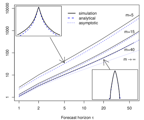
Figure 12: Error growth for large simulations of a IMA(1,1) process, to check Eq. (14) and (15). Simulations are done using 5000 time series of 100 periods, all with with $\mu=0.04$, $K=0.05$, $\theta=0.6$. The insets show the distribution of forecast errors, as in Fig. 8, for $m=5,40$

To obtain the results with estimated (instead of true) variance (Eq. (14) and (15)), we follow the same procedure as in Appendix B.1, which assumes independence between the error and the estimated variance. Fig. 12 shows that the result is not exact but works reasonably well if $m>15$.

Appendix C Robustness checks

C.1 Size of the learning window

As a check on the results presented in Section 5.3 we test the dependence of the forecast errors on the sample window $m$ for several different forecast horizons. The results are robust to a change of the size of learning window $m$. It is not possible to go below $m=4$ because when $m=3$ the Student distribution has $m-1=2$ degrees of freedom, hence an infinite variance. Note that to make forecasts using a large $m$ only the datasets which are long enough can be included. The results for a few values of $m$ are shown in Fig. 9. Fig. 13 shows that the normalized mean squared forecast error consistently decreases as the learning window increases.

Figure 13: Empirical mean squared normalized forecast errors as a function of the size of learning window for different forecast horizons. The dots are the empirical errors and the plain lines are those expected if the true model was an IMA(1,1) with $\theta_{m}=0.63$.

C.2 Data selection

We have checked how the results change when about half of the technologies are randomly selected and removed from the dataset. The shape of the normalized mean squared forecast error growth does not change and is shown in Fig. 14. The procedure is based on 10000 random trials selecting half the technologies.

Figure 14: Robustness to dataset selection. Mean squared normalized forecast errors as a function of $\tau$ when using only half of the technologies (26 out 53), chosen at random. The 95% confidence intervals, shown as dashed lines, are for the mean squared normalized forecast errors when we randomly select 26 technologies.

C.3 Increasing $\tau_{max}$

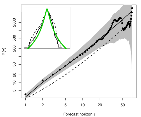
Figure 15: Robustness to increasing $\tau_{max}$. Main results (i.e as in Fig. 6 and 8) using $\tau_{max}=73$. We use $\theta=0$ and $\theta=0.63$.

In the main text we have shown the results for a forecast horizon up to $\tau_{max}=20$. Moreover, we have used only the forecast errors up to $\tau_{max}$ to construct the empirical distribution of forecast errors in Fig. 8 and to estimate $\theta$ in Appendix D. Fig. 15 shows that if we use all the forecast errors up to the maximum with $\tau=73$ the results do not change significantly.

C.4 Heavy tail innovations

To check the effect of non-normal noise increments on $\Xi(\tau)$ we simulated random walks with drift with noise increments drawn from a Student distribution with 3 or 7 degrees of freedom. Fig. 16 shows that fat tail noise increments do not change the long horizon errors very much. While the IMA(1,1) model produces a parallel shift of the errors at medium to long horizons, the Student noise increments generate larger errors mostly at short horizons. Thus fat-tail innovations are not the most important source of discrepancy between the geometric random walk model and the empirical data.

Figure 16: Effect of fat tail innovations on error growth. The figure shows the growth of the mean squared normalized forecast errors for four models, showing that introducing fat tail innovations in a random walk with drift (RWD) mostly increases errors only at short horizons.

Appendix D Procedure for selecting the autocorrelation parameter $\theta$

Figure 17: Estimation of $\theta$ as a global parameter

Figure 18: Using the IMA model to make better forecasts. The right panel uses $\theta=0.25$

We select $\theta$ in several ways. The first method is to compute a variety of weighted means for the $\tilde{\theta}_{j}$ estimated on individual series. The main problem with this approach is that for some technology series the estimated $\theta$ was very close to 1 or -1, indicating mis-specification or estimation problems. After removing these 8 technologies the mean with equal weights for each technology is $0.27$ with standard deviation $0.35$. We can also compute the weighted mean at each forecast horizon, with the weights being equal to the share of each technology in the number of forecast errors available at a given forecast horizon. In this case the weighted mean $\theta_{w}(\tau)$ will not necessarily be constant over time. Fig. 17 (right) shows that $\theta_{w}(\tau)$ oscillates between 0.24 and 0.26. Taking the average over the first 20 periods gives $\theta_{w}=\frac{1}{20}\sum_{\tau=1}^{20}\theta_{w}(\tau)=0.25$. When doing this we do not mean to imply that our formulas are valid for a system with heterogenous $\theta_{j}$; we simply propose a best guess for a universal $\theta$.

The second approach is to select $\theta$ in order to match the errors. As before we generate many artificial data sets using the IMA(1,1) model. Larger values of $\theta$ imply that using the simple random walk model to make the forecasts will result in higher forecast errors. Denote by $\Xi(\tau)_{empi}$ the empirical mean squared normalized forecast error as depicted in Fig. 6, and by $\Xi(\tau)_{sim,\theta}$ the expected mean squared normalized forecast error obtained by simulating IMA(1,1) datasets 3,000 times with a particular global value of $\theta$ and taking the average. We study the ratio of these two, averaged over all $1\dots\tau_{max}=20$ periods, i.e. $Z(\theta)=\frac{1}{20}\sum_{\tau=1}^{20}\frac{\Xi(\tau)_{empi}}{\Xi(\tau)_{sim,\theta}}.$ The values are shown in Fig. 17 (left). The value at which $|Z-1|$ is minimum is at $\theta_{m}=0.63$.

We also tried to make forecasts using the IMA model to check that forecasts are improved: which value of $\theta$ allows the IMA model to produce better forecasts? We apply the IMA(1,1) model with different values of $\theta$ to make forecasts (with the usual estimate of the drift term $\hat{\mu}$) and study the normalized error as a function of $\theta$. We record the mean squared normalized error and repeat this exercise for a range of values of $\theta$. The results for horizons 1,2, and 10 are reported in Fig. 18 (left). This shows that the best value of $\theta$ depends on the time horizon $\tau$. The curve shows the mean squared normalized forecast error at a given forecast horizon as a function of the value of $\theta$ assumed to make the forecasts. The vertical lines show the minima at 0.26, 0.40, and 0.66. Given that the mean squared normalized forecast error increases with $\tau$, to make the curves fit on the plot the values are normalized by the mean squared normalized forecast error using $\theta=0$. We also see that as the forecast horizon increases the improvement from taking the autocorrelation into account decreases (Fig. 18, right), as expected theoretically from an IMA process. Note that the improvement in forecasting error is only a few percent, even for $\tau=1$, indicating that this makes little difference.

Appendix E Comparison of the empirical distribution of rescaled errors to the predicted Student distribution

In this section we check whether the deviations of the empirical forecast errors from the predicted theoretical distribution shown in Fig. 8 are consistent with statistical sampling error. For a given value of $\theta$ we generate a surrogate data set and surrogate forecasts mimicking our empirical data as described at the end of Section 4.1. We then construct a sample surrogate (cumulative) distribution $P_{k}$ for the pooled rescaled errors $\epsilon^{*}$ of Eq. (15). We measure the distribution $P_{k}$ over 1,000 equally spaced values $x_{k}$ on the interval $[-15;15]$. $P_{k}$ is estimated by simply counting the number of observations less than $x_{k}$. This is then compared to the predicted Student distribution $t_{k}$ by computing the difference $\Delta_{k}=P_{k}-t_{k}$ between the surrogate distribution and the Student distribution in each interval. We measure the overall deviation between the surrogate and the Student using three different measures of deviation: $\sum_{k}|\Delta_{k}|$, $\sum_{k}(\Delta_{k})^{2}$, and $\max\Delta_{k}$. We then repeat this process 10,000 times to generate a histogram for each of the measures above, and compare this to the measured value of the deviation for the real data.

Results for doing this for $\theta_{w}=0.25$ and $\theta_{m}=0.63$ are reported in Fig. 19. For $\theta_{w}$ the resulting $p$-values (the shares of random datasets with a deviation higher than the empirical deviation) are $(0.001,0.002,0.011)$ respectively using $(\sum_{k}|\Delta_{k}|$, $\sum_{k}(\Delta_{k})^{2}$, $\max\Delta_{k})$ to measure the deviation. In contrast for $\theta_{m}=0.63$ the $p$-values are $(0.21,0.16,0.20)$. Thus $\theta_{m}=0.63$ is accepted and $\theta_{w}=0.25$ is rejected. The uncorrelated case $\theta=0$ is rejected even more strongly.

Figure 19: Expected deviations of the distribution of the rescaled variable $\epsilon^{*}$ of Eq. (15) from the Student distribution for hindcasting experiments as we do here using a dataset with the same properties as ours. The histograms show the sampling distribution of a given statistic and the thick black line shows the empirical value on real data. The simulations use $\theta=0.25$ (3 upper panels) and $\theta=0.63$ (3 lower panels).

Appendix F A trend extrapolation of solar energy capacity

In this paper we have been concerned with forecasting costs. For some applications it is also useful to forecast production. Our exploratory work so far suggests that, while the same basic methods can be applied, production seems more likely to deviate systematically from increasing exponentially. Nonetheless, Nagy et al. (2013) found that as a rough approximation most of the technologies in our data set can be crudely (but usefully) approximated as having exponentially increasing production for a long span of their development cycle, and solar PV is no exception. Trend extrapolation can add perspective, even if it comes without good error estimates, and the example we present below motivates the need for more work to formulate better methods for assessing the reliability of production forecasts (for an example, see Shlyakhter et al. (1994)).

Many analysts have expressed concerns about the time required to build the needed capacity for solar energy to play a role in reducing greenhouse gas emissions. The "hi-Ren" (high renewable) scenario of the International Energy Agency assumes that PV will generate $16\%$ of total electricity in 2050; this was recently increased from the previous estimate of only $11\%$. As a point of comparison, what do past trends suggest?

Though estimates vary, over the last ten years cumulative installed capacity of PV has grown at an impressive rate. According to BP’s Statistical Review of World Energy 2014, during the period from 1983-2013 solar energy as a whole grew at an annual rate of 42.5% and in 2014 represented about 0.22% of total primary energy consumption, as shown in Fig. 20. By comparison total primary energy consumption grew at an annual rate of 2.6% over the period 1965-2013. Given that solar energy is an intermittent source, it is much easier for it to contribute when it supplies only a minority of energy: new supporting technologies will be required once it becomes a major player. If we somewhat arbitrarily pick $20\%$ as a target, assuming both these trends continue unaltered, a simple calculation shows that this would be achieved in about 13.7 years. That is, under these assumptions in 2027 solar would represent $20\%$ of energy consumption. Of course this is only an extrapolation, but it puts into perspective claims that solar energy cannot play an essential role in mitigating global warming on a relatively short timescale.

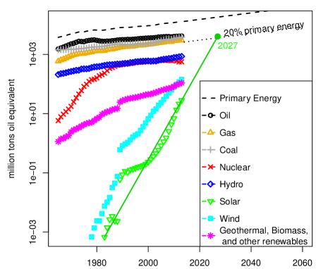
Figure 20: Global energy consumption due to each of the major sources from BP Statistical Review of World Energy (BP, 2014). Under a projection for solar energy obtained by fitting to the historical data the target of $20\%$ of global primary energy is achieved in 2027.

Of course the usual caveats apply, and the limitations of such forecasting is evident in the historical series of Fig. 20. The increase of solar is far from smooth, wind has a rather dramatic break in its slope in roughly 1988, and a forecast for nuclear power made in 1980 based on production alone would have been far more optimistic than one today. It would be interesting to use a richer economic model to forecast cost and production simultaneously, but this is beyond the scope of this paper. The point here was simply to show that if growth trends continue as they have in the past significant contributions by solar are achievable.

References

- (1)
- Alberth (2008) Alberth, S. (2008), ‘Forecasting technology costs via the experience curve: Myth or magic?’, Technological Forecasting and Social Change 75(7), 952–983.
- Albright (2002) Albright, R. E. (2002), ‘What can past technology forecasts tell us about the future?’, Technological Forecasting and Social Change 69(5), 443–464.
- Alchian (1963) Alchian, A. (1963), ‘Reliability of progress curves in airframe production’, Econometrica 31(4), 679–693.
- Argote & Epple (1990) Argote, L. & Epple, D. (1990), ‘Learning curves in manufacturing’, Science 247(4945), 920–924.
- Arrow (1962) Arrow, K. J. (1962), ‘The economic implications of learning by doing’, The Review of Economic Studies 29(3), 155–173.
- Ayres (1969) Ayres, R. U. (1969), ‘Technological forecasting and long-range planning’.
- Bailey et al. (2012) Bailey, A., Bui, Q. M., Farmer, J., Margolis, R. & Ramesh, R. (2012), Forecasting technological innovation, in ‘ARCS Workshops (ARCS), 2012’, pp. 1–6.
- Baker et al. (2013) Baker, E., Fowlie, M., Lemoine, D. & Reynolds, S. S. (2013), ‘The economics of solar electricity’, Annual Review of Resource Economics 5, 387–426.
- Barbose et al. (2014) Barbose, G., Darghouth, N., Weaver, S. & Wiser, R. (2014), Tracking the Sun VI: An Historical Summary of the Installed Price of Photovoltaics in the United States from 1998 to 2012, NREL.
- Benson & Magee (2014a) Benson, C. L. & Magee, C. L. (2014a), ‘On improvement rates for renewable energy technologies: Solar PV, wind turbines, capacitors, and batteries’, Renewable Energy 68, 745–751.
- Benson & Magee (2014b) Benson, C. L. & Magee, C. L. (2014b), ‘Quantitative determination of technological improvement from patent data’, ESD Working Paper Series 2014-29.
- Blough (1992) Blough, S. R. (1992), ‘The relationship between power and level for generic unit root tests in finite samples’, Journal of Applied Econometrics 7(3), 295–308.
- Bosetti et al. (2012) Bosetti, V., Catenacci, M., Fiorese, G. & Verdolini, E. (2012), ‘The future prospect of pv and csp solar technologies: An expert elicitation survey’, Energy Policy 49, 308–317.
- Boston Consulting Group (1972) Boston Consulting Group (1972), Perspectives on Experience, 3 edn, The Boston Consulting Group, Inc., One Boston Place, Boston, Massachusetts 02106.
- Box & Jenkins (1970) Box, G. E. & Jenkins, G. M. (1970), Time Series Analysis: Forecasting and Control, Holden-Day, San Francisco.
-
BP (2014)
BP (2014), ‘BP statistical review of world
energy’.
http://www.bp.com/en/global/corporate/about-bp/energy-economics/statistical-review-of-world-energy.html - Chatfield (1993) Chatfield, C. (1993), ‘Calculating interval forecasts’, Journal of Business & Economic Statistics 11(2), 121–135.
- Clements & Hendry (2001) Clements, M. P. & Hendry, D. F. (2001), ‘Forecasting with difference-stationary and trend-stationary models’, Econometrics Journal 4(1), 1–19.
- Colpier & Cornland (2002) Colpier, U. C. & Cornland, D. (2002), ‘The economics of the combined cycle gas turbine, an experience curve analysis’, Energy Policy 30(4), 309–316.
- Cooper (2009) Cooper, M. (2009), The economics of nuclear reactors: Renaissance or relapse, Technical report, Vermont Law School.
- Curtright et al. (2008) Curtright, A. E., Morgan, M. G. & Keith, D. W. (2008), ‘Expert assessments of future photovoltaic technologies’, Environmental Science & Technology 42(24), 9031–9038.
- Dutton & Thomas (1984) Dutton, J. M. & Thomas, A. (1984), ‘Treating progress functions as a managerial opportunity’, Academy of Management Review 9(2), 235–247.
- Funk (2013) Funk, J. L. (2013), ‘What drives exponential improvements?’, California Management Review 55(3), 134–155.
- Funk & Magee (2014) Funk, J. L. & Magee, C. L. (2014), ‘Rapid improvements with no commercial production: How do the improvements occur?’, Research Policy .
- Goddard (1982) Goddard, C. (1982), ‘Debunking the learning curve’, Components, Hybrids, and Manufacturing Technology, IEEE Transactions on 5(4), 328–335.
- Goldemberg et al. (2004) Goldemberg, J., Coelho, S. T., Nastari, P. M. & Lucon, O. (2004), ‘Ethanol learning curve, the Brazilian experience’, Biomass and Bioenergy 26(3), 301–304.
- Gordon (1990) Gordon, R. J. (1990), The Measurement of Durable Goods Prices, University of Chicago Press.
- International Energy Agency (2014) International Energy Agency (2014), Technology roadmap: Solar photovoltaic energy (2014 ed.), Technical report, OECD/IEA, Paris.
- Jamasb (2007) Jamasb, T. (2007), ‘Technical change theory and learning curves: patterns of progress in electricity generation technologies’, The Energy Journal 28(3), 51–71.
- Jantsch (1967) Jantsch, E. (1967), Technological forecasting in perspective, OCDE.
- Koh & Magee (2006) Koh, H. & Magee, C. L. (2006), ‘A functional approach for studying technological progress: Application to information technology’, Technological Forecasting and Social Change 73(9), 1061–1083.
- Koh & Magee (2008) Koh, H. & Magee, C. L. (2008), ‘A functional approach for studying technological progress: Extension to energy technology’, Technological Forecasting and Social Change 75(6), 735–758.
- Koomey & Hultman (2007) Koomey, J. & Hultman, N. E. (2007), ‘A reactor-level analysis of busbar costs for US nuclear plants, 1970–2005’, Energy Policy 35(11), 5630 – 5642.
- Kost et al. (2013) Kost, C., Mayer, J., Thomsen, J., Hartmann, N., Senkpiel, C., Philipps, S., Nold, S., Lude, S., Saad, N. & Schleg, T. L. (2013), Levelized cost of electricity: Renewable energy technologies., Technical report, Fraunhofer Institute for Solar Energy Systems.
- Lee & Scholtes (2014) Lee, Y. S. & Scholtes, S. (2014), ‘Empirical prediction intervals revisited’, International Journal of Forecasting 30(2), 217–234.
- Lieberman (1984) Lieberman, M. B. (1984), ‘The learning curve and pricing in the chemical processing industries’, The RAND Journal of Economics 15(2), 213–228.
- Lienhard (2006) Lienhard, J. H. (2006), How invention begins: Echoes of old voices in the rise of new machines, Oxford University Press.
- Lipman & Sperling (1999) Lipman, T. E. & Sperling, D. (1999), ‘Experience curves for policy making: the case of energy technologies’.
- Makridakis & Winkler (1989) Makridakis, S. & Winkler, R. L. (1989), ‘Sampling distributions of post-sample forecasting errors’, Applied Statistics 38(2), 331–342.
- Martino (1993) Martino, J. P. (1993), Technological forecasting for decision making, McGraw-Hill, Inc.
- McDonald & Schrattenholzer (2001) McDonald, A. & Schrattenholzer, L. (2001), ‘Learning rates for energy technologies’, Energy Policy 29(4), 255–261.
- McNerney et al. (2011) McNerney, J., Farmer, J. D. & Trancik, J. E. (2011), ‘Historical costs of coal-fired electricity and implications for the future’, Energy Policy 39(6), 3042–3054.
- Moore (2006) Moore, G. E. (2006), ‘Behind the ubiquitous microchip’.
- Nagy et al. (2013) Nagy, B., Farmer, J. D., Bui, Q. M. & Trancik, J. E. (2013), ‘Statistical basis for predicting technological progress’, PloS one 8(2), e52669.
- Nagy et al. (2011) Nagy, B., Farmer, J. D., Trancik, J. E. & Gonzales, J. P. (2011), ‘Superexponential long-term trends in information technology’, Technological Forecasting and Social Change 78(8), 1356–1364.
- National Research Council (2009) National Research Council (2009), Persistent Forecasting of Disruptive Technologies., The National Academies Press.
- Neij et al. (2003) Neij, L., Andersen, P. D., Durstewitz, M., Helby, P., Hoppe-Kilpper, M. & Morthorst, P. (2003), Experience curves: A tool for energy policy assessment, Environmental and Energy Systems Studies, Univ.
- Nemet (2006) Nemet, G. F. (2006), ‘Beyond the learning curve: factors influencing cost reductions in photovoltaics’, Energy Policy 34(17), 3218–3232.
- Nordhaus (2007) Nordhaus, W. D. (2007), ‘Two centuries of productivity growth in computing’, The Journal of Economic History 67(01), 128–159.
- Nordhaus (2009) Nordhaus, W. D. (2009), The perils of the learning model for modeling endogenous technological change, Technical report, National Bureau of Economic Research.
- Perlin (1999) Perlin, J. (1999), From space to earth: the story of solar electricity, Earthscan.
- Sampson (1991) Sampson, M. (1991), ‘The effect of parameter uncertainty on forecast variances and confidence intervals for unit root and trend stationary time-series models’, Journal of Applied Econometrics 6(1), 67–76.
- Schilling & Esmundo (2009) Schilling, M. A. & Esmundo, M. (2009), ‘Technology s-curves in renewable energy alternatives: Analysis and implications for industry and government’, Energy Policy 37(5), 1767 – 1781.
- Shlyakhter et al. (1994) Shlyakhter, A. I., Kammen, D. M., Broido, C. L. & Wilson, R. (1994), ‘Quantifying the credibility of energy projections from trends in past data: The us energy sector’, Energy Policy 22(2), 119–130.
- Sinclair et al. (2000) Sinclair, G., Klepper, S. & Cohen, W. (2000), ‘What’s experience got to do with it? sources of cost reduction in a large specialty chemicals producer’, Management Science 46(1), 28–45.
- Taylor & Bunn (1999) Taylor, J. W. & Bunn, D. W. (1999), ‘A quantile regression approach to generating prediction intervals’, Management Science 45(2), 225–237.
- Thompson (2012) Thompson, P. (2012), ‘The relationship between unit cost and cumulative quantity and the evidence for organizational learning-by-doing’, The Journal of Economic Perspectives 26(3), 203–224.
-
Wetterstrand (2015)
Wetterstrand, K. (2015), ‘DNA sequencing
costs: Data from the NHGRI genome sequencing program (GSP)’.
www.genome.gov/sequencingcosts - Williams & Goodman (1971) Williams, W. & Goodman, M. (1971), ‘A simple method for the construction of empirical confidence limits for economic forecasts’, Journal of the American Statistical Association 66(336), 752–754.
- Working (1960) Working, H. (1960), ‘Note on the correlation of first differences of averages in a random chain’, Econometrica 28(4), pp. 916–918.
- Wright (1936) Wright, T. P. (1936), ‘Factors affecting the cost of airplanes’, Journal of the Aeronautical Sciences 3(4), 122—128.
- Zhao (1999) Zhao, J. (1999), ‘The diffusion and costs of natural gas infrastructures’.