Antiferromagnetic metal phases in double perovskites having strong antisite defect concentrations

Abstract

Recently an antiferromagnetic metal phase has been proposed in double perovskites materials like Sr₂FeMoO₆ (SFMO), when electron doped. This material has been found to change from half-metallic ferromagnet to antiferromagnetic metal (AFM) upon La-overdoping. The original proposition of such an AFM phase was made for clean samples, but the experimental realization of La-overdoped SFMO has been found to contain a substantial fraction of antisite defects. A phase segregation into alternate Fe and Mo rich regions was observed. In this paper we propose a possible scenario in which this type of strong antisite concentration can still result in an antiferromagnetic metal phase, by a novel hopping driven mechanism. Using variational calculations, we find that proliferation of such phase segregated domain regions can also result in the stabilization of an A-type AFM over the G-type AFM based on kinetic energy considerations.

I Introduction

Double perovskites, with the general formula A₂BB^′O₆, A=alkaline/rare-earth metals and B/B^′=transition metals, are being studied extensively in recent years due to their half-metallic properties tomioka ; TSD , and their importance in spintronic applications. A prominent member, Sr₂FeMoO₆, is ferromagnetic in the pure state with a $T_{c}$ as high as 410K. SFMO ; DDreview . Substantial tunnelling magnetoresistance is also obtained in powdered samples of these compounds at low temperatures.  SFMO ; Mag-Res1 ; Mag-Res2 ; MRpaper . There is a kind of defect which is possible in double perovskite materials called antisite defects in which a B-atom (Fe) and a B${}^{{}^{\prime}}$ atom (Mo) can interchange position, thereby bringing two B (Fe) atoms next to each other. Such defect regions tend to be antiferromagnetic and insulating, and decrease the overall magnetization. While tunneling across grain boundaries, rather than antisite regions dominates as the main mechanism for magnetoresistance, the magnitude of the magnetoresistance does get affected quite dramatically by the antisite defect concentration. MRpaper . Attempts have been made to electron dope this compound (SFMO) hoping to enhance the $T_{c}$ and hence the polarization at room temperature and thereby improve the magnetoresistance. JAP ; ES ; Navarro ; photoemission . While a slight increase in $T_{c}$ is indeed observed for low dopings Navarro ; p21n , but for overdoping ($x>1$), the $T_{c}$ is found to decrease,as shown in mePinaki ; LSFMO , and the ferromagnetism gets replaced by antiferromagnetic phases. These antiferromagnetic phases are however, metallic, and are stabilized over the ferromagnetic phase due to a kinetic energy-driven mechanism. This was derived using a model Hamiltonian in the clean limit without antisite defects, using analytical as well as numerical methods mePinaki . Further confirmation was obtained using abinitio methods, by considering the Sr_2-xLa_xFeMoO₆ series LSFMO , for the overdoped case ($x>1$). In the actual experimental preparation of this proposed series of materials, however, substantial concentration of antisite defects was found to be present Sugatapriv . In fact, a microscopic phase segregation situation was encountered, where the sample phase segregated into alternate Fe-rich and Mo-rich regions, forming a patchy structure. In this paper, using a variational approach, we reconsider the stability of magnetic phases in presence of antisite defects, and in particular in the phase segregation scenario where alternate Fe-rich and Mo-rich regions are present. We find that antiferromagnetic metal phases are still stabilized kinetically for large regions of filling. The exact nature of the kinetically stabilized antiferromagnetic phase, however, changes from the clean limit to the alternate Fe-Mo rich phase segregated scenario. We confirm this change using numerical simulations based on exact diagonalization, where phase segregated Fe-Mo domains are allowed to proliferate over an otherwise clean sample. Our results are in consonance with those of an earlier study in presence of antisite defects using a different method, where it was found that antiferromagnetic phases do survive even in presence of antisite disorder VSinghPinaki . Although they considered correlated antisite disorder, they did not consider alternate Fe-Mo rich regions or phase segregation. We have obtained analytical results in the phase segregated limit, using a variational approach. The organization of the paper is as follows. In the next section, we shall briefly summarize the experimental results for the Sr_2-xLa_xFeMoO₆ series (i.e., cataion site substitution), and the role of antisite defects. Next, we discuss a Hamiltonian suitable for analyzing this problem including antisite defects. In the next section, we consider the results. First we consider a fully phase segregated situation with alternate Fe-rich and Mo-rich segments, using analytical variational methods. Then we proceed to consider a generic situation where Fe-rich and Mo-rich domains are allowed to form inside an otherwise clean sample with rocksalt structure. Using exact diagomalization methods, we then consider the proliferation of such domains inside the sample.

II Experimental data on La-doped SFMO: Brief summary

Experimental attempts at electron doping Sr₂FeMoO₆ by substituting Sr²⁺ with La³⁺ had been ongoing for a while JAP ; Navarro . This results in the series of compounds Sr_2-xLa_xFeMoO₆. While some of these authors have reported that the samples retained tetragonal symmetry (I4/mmm) upon electron doping from x=0 all the way upto x=1, others report a change to monoclinic symmetry (P2₁/n) upon doping beyond x=0.4. However, all the authors consent on the fact that the cell parameters increase upon doping, and the antisite defect concentration increases, thereby reducing the degree and extent of ordering. This can be understood by considering the behaviour of the saturation magnetization, and comparing with abinitio calculations. Such calculations indicate that the half-metallic behaviour persists from Sr₂FeMoO₆ till SrLaFeMoO₆ (LSFMO) JAP ; LSFMO , and the total moment changes from 4$\mu_{B}$/f.u. to 3$\mu_{B}/f.u.$, i.e., a reduction in moment by 1$\mu_{B}/f.u.$ by doping by $x=1$, in the clean limit. This is due to the fact that a replacement of Sr²⁺ ion by La³⁺ ion due to La-doping results in the addition of an electron into the cell, and since LSFMO is half-metallic, the extra electron goes into the minority spin band, reducing the moment by exactly 1$\mu_{B}$. The experimental reduction, on the other hand, is by 2$\mu_{B}$/f.u. JAP , for example, clearly indicating the increase in concentration of antisite defects, along with the electron doping effect. Such increase in antisite defect concentration has been confirmed in almost all the studies, even leading to a concentration level of $0.5$ in some cases for $x>0.8$ Navarro , where a phase separation scenario is possible.

Recently, there has been a study of La-overdoping of Sr₂FeMoO₆, where the regime above $x>1$ is investigated Sugatapriv . As before, increase in antisite disorder with increasing doping is observed. However, the sample is found to phase segregate into alternate Sr,Mo-rich and La,Fe-rich short range patches, which is confirmed by X-ray spectra analysis. The number of Mo-O-Mo connections, which should be 0 for a perfectly ordered arrangement, 3 for a random situation, and 6 for a phase segregation scenario, was found to be more than 3, while the samples crystallized to a space group of P$2_{1}$/n, indicating a patchy structure as mentioned before. Interestingly, even with this heavy concentration of antisite disorder, the samples remained metallic, although there was a transition from ferromagnetic to antiferromagnetic phase, as evidenced from magnetization hysteresis data. Thus, a rare antiferromagnetic metallic phase appears to be stabilized for an overdoped, phase-segregated sample of SFMO. In this paper we provide a plausible explanation to such a situation using model Hamiltonian methods. While a crossover from ferromagnetic metal phase to an antiferromagnetic metal phase has already been predicted in the clean limit without antisites mePinaki ; LSFMO , in this paper we consider the case with antisite defects, in particular a phase segregation scenario, and justify how this crossover can continue to hold even in this scenario.

III Hamiltonian

A Hamiltonian suitable for considering general Fe-Mo configurations with antisite defects can be obtained in the following way vivekanand ; VSinghPinaki , by considering a local binary variable $\eta_{i}$ which is $1$ or $0$ depending on whether the site is Fe or Mo:

$$H=\epsilon_{Fe}\sum_{i,\sigma}\eta_{i}f_{i\sigma}^{\dagger}f_{i\sigma}+\epsilon_{Mo}\sum_{i,\sigma}(1-\eta_{i})m_{i\sigma}^{\dagger}m_{i\sigma}$$

$$+t_{FF}\sum_{<ij>\sigma}\eta_{i}\eta_{j}f_{i\sigma}^{\dagger}f_{j\sigma}+t_{MM}\sum_{<ij>\sigma}(1-\eta_{i})(1-\eta_{j})m_{i\sigma}^{\dagger}m_{j\sigma}$$

$$+t_{FM}\sum_{<ij>\sigma}(\eta_{i}+\eta_{j}-2\eta_{i}\eta_{j})f_{i\sigma}^{\dagger}m_{j\sigma}$$

$$+J\sum_{i\alpha\beta}\eta_{i}{\bf S}_{i}\cdot f_{i\alpha}^{\dagger}\vec{\sigma}_{\alpha\beta}f_{i\beta}+J_{AF}\sum_{<ij>}\eta_{i}\eta_{j}S_{i}\cdot S_{j}$$ (1)

The $f$’s refer to the Fe sites and the $m$’s to the Mo sites. $t_{FM}$, $t_{MM}$, $t_{FF}$ represent the nearest neighbor Fe-Mo, Mo-Mo and Fe-Fe hoppings respectively. $\sigma$ is the spin index. The difference between the ionic levels, ${\tilde{\Delta}}=\epsilon_{Fe}-\epsilon_{Mo}$, defines the charge transfer energy. The ${\bf S}_{i}$ are ‘classical’ (large $S$) core spins at the B site, coupled to the itinerant B electrons through a coupling $J\gg t_{FM}$. Each $\{\eta_{i}\}$ realization corresponds to a configuration of antisite disorder; in particular, the ordered configuration (without antisite defects) corresponds to a checkerboard, or $[\pi,\pi]$ configuration of $\eta_{i}$ on a 2D lattice. The model then coincides with the two-sublattice Kondo lattice model which has been considered by several authors Millis ; Avignon ; Guinea1 ; Guinea2 in the context of ordered double perovskites. If one considers the limit $J\rightarrow\infty$, then the model given by Eq 1 simplifies to a model with “spinless” Fe degrees of freedom Guinea1 ; Guinea2 :

$$H = t_{FM}\sum_{<ij>\alpha}(\eta_{i}+\eta_{j}-2\eta_{i}\eta_{j})(sin(\frac{\theta_{i}}{2})\tilde{f}_{i}^{\dagger}m_{j\uparrow}$$ (7)

$$-e^{i\phi_{i}}cos(\frac{\theta_{i}}{2})\tilde{f}^{\dagger}_{i}m_{j\downarrow})$$

$$+h.c.+t_{MM}\sum_{<ij>}(1-\eta_{i})(1-\eta_{j})m_{i\sigma}^{\dagger}m_{j\sigma}$$

$$+t_{FF}\sum_{<ij>}\eta_{i}\eta_{j}cos(\theta_{ij}/2)(\tilde{f}_{i}^{\dagger}\tilde{f}_{j})$$

$$+\tilde{\epsilon_{Fe}}\sum_{i}\eta_{i}\tilde{f}_{i}^{\dagger}\tilde{f}_{i}+\epsilon_{Mo}\sum_{i\sigma}(1-\eta_{i})m_{i\sigma}^{\dagger}m_{i\sigma}$$

$$+J_{AF}\sum_{<ij>}\eta_{i}\eta_{j}S_{i}\cdot S_{j}$$

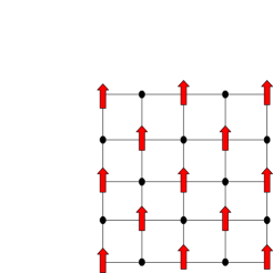
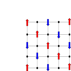
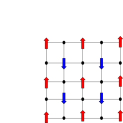
Figure 1: The three magnetic phases in the ordered 2D model. Arrows represent Fe sites, and dots Mo sites.
Left: ferromagnetic (FM), center: antiferromagnet (AFM1), right: antiferromagnet (AFM2). The moments are on the B sites.

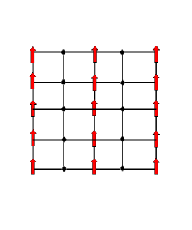
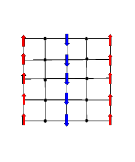
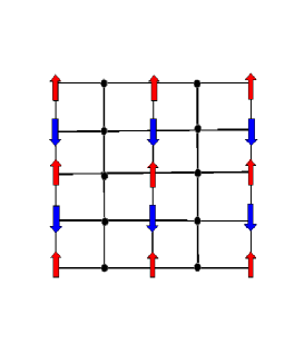
Figure 2: The three magnetic phases in the phase segregated case: alternate Fe and Mo-rich regions. Arrows represent Fe sites, and the dots Mo sites.
Left: ferromagnetic (FM), center: antiferromagnet (AFM1), right: antiferromagnet (AFM2).

In the ordered case, this model has been studied as a function of filling of the Fe and Mo degrees of freedom, using various analytical and numerical methods mePinaki . It was found that while a ferromagnetic phase was stable for low fillings $n<1$, it became unstable to antiferromagnetic phases for larger filling $n>1$. There appeared to be two main types of antiferromagnetic phases: A type ($0-\pi$) or AFM1, and G type ($\pi-\pi$) phases, or AFM2. A schematic of these three phases are shown in Fig 1.

IV Alternate Phase segregated case

Samples of La-overdoped SFMO are found to order in a patchy structure Sugatapriv where phase segregation occurs into alternate Fe-rich and Mo-rich regions. This leads to a substantial amount of antisite defects. The simplest model for this situation can be considered in 2D as follows. Let us consider strips of Fe and Mo atoms arranged alternately as shown in Fig 2, or in the bottom panel of Fig 4. This would mean alternate lines of antisite defects separated from each other by patches where Fe and Mo are nearest neighbour. Such a patchy structure can be used to effectively describe the samples of Sr_2-xLa_xFeMoO₆. This configuration can be thought to be realized from an ordered checkerboard configuration of Fe, Mo by proliferation of domain line-defects of Fe and Mo combined. Accordingly, the ferromagnetic, A type antiferromagnet and G type antiferromagnet can be realized in the the form shown in Fig 2. In this case, the dispersions in the three phases can be calculated as follows. In the fully ferromagnetic case, the dispersion is given by:

$$\epsilon_{k} = \frac{[\epsilon_{Fe}+\epsilon_{Mo}+2(t_{FF}+t_{MM})cosky]\pm\sqrt{[(\epsilon_{Fe}+2t_{FF}cosky)-(\epsilon_{Mo}+2t_{MM}cosky)]^{2}+16t_{FM}^{2}cos^{2}kx}}{2}$$ (8)

If we put $t_{FF}=t_{MM}=0$, then

$$\epsilon_{k}=\frac{(\epsilon_{Fe}+\epsilon_{Mo})\pm\sqrt{(\epsilon_{Fe}-\epsilon_{Mo})^{2}+16t_{FM}^{2}cos^{2}kx}}{2}$$ (9)

which is just the band structure of a 1D binary lattice, appropriate for the isolated Fe-Mo alternating chains in the x-direction (to the right). If $\epsilon_{Fe}=\epsilon_{Mo}=0$, then $\epsilon_{k}=\pm 2t_{FM}coskx$, revealing the 1D character. If we put $t_{FM}=0$, then we get, for $\epsilon_{Fe}=\epsilon_{Mo}=0$, $\epsilon_{k}^{+}=2t_{FF}cosky$ and $\epsilon_{k}^{-}=2t_{MM}cosky$, once again 1D band structures, this time in the y direction, as expected.

For the antiferromagnetic cases, the dispersions are obtained in the following manner. For the A-type antiferromagnet, there are alternate ferromagnetic chains arranged antiferromagnetically. This can be obtained in the phase segregated limit by considering the fact that in the ordered phase (as shown in the central panel of Fig 1), the up and down spins alternate on the Fe sites on any line along the x-direction, separated by an Mo site. Since this structure is preserved by a Fe-Mo line domain shift in the x-direction, the resulting phase is as shown in the central panel of Fig 2. The dispersion is given by $\epsilon_{k}=\epsilon_{Mo}+2t_{MM}cosky$ and

$$\epsilon_{k}=\frac{[\epsilon_{Fe}+\epsilon_{Mo}+2(t_{FF}+t_{MM})cosky]\pm\sqrt{[(\epsilon_{Fe}+2t_{FF}cosky)-(\epsilon_{Mo}+2t_{MM}cosky)]^{2}+8t_{FM}^{2}}}{2}$$ (10)

If we consider $t_{FF}=t_{MM}=0$, and $\epsilon_{Fe}=\epsilon_{Mo}=0$, then the dispersion simplifies to just three possible values: $0,\pm\sqrt{2}t_{FM}$ appropriate for a triatomic molecule, as expected for an Mo-Fe-Mo trimer. If $t_{FM}=0$, then it gives the 1D dispersions $\epsilon_{Fe}+2t_{FF}cosky$ and $\epsilon_{Mo}+2t_{MM}cosky$, corresponding to 1D Fe chains and Mo chains in the y-direction as expected.

The G-type antiferromagnet, which corresponds to the $\pi-\pi$ antiferromagnet for the ordered lattice, can be realized in this antisite disordered case by considering the fact that along a line in the x-direction, in the ordered phase, the Iron spins all remain parallel (see right panel of Fig 1). Since this is once again preserved during a Fe-Mo line domain shift in the x-direction, hence the spin configuration that is realized is as shown in the right panel of Fig 2. Here the Iron spins are parallel along the x-direction, while they alternate antiparallely along the y-direction. In this case, the dispersion is obtained as the roots of a cubic equation:

$$(\epsilon_{Fe}-\epsilon_{k})(\epsilon_{Mo}-\epsilon_{k})^{2}-(\epsilon_{Fe}-\epsilon_{k})t_{MM}^{2}(2+2cosky)-t_{FM}^{2}(2+2coskx)(\epsilon_{Mo}-\epsilon_{k})=0$$ (11)

The limits can be obtained exactly. For example if $t_{MM}=0$, $\epsilon_{k}=\epsilon_{Mo}$ (the isolated Mo level) and

$$\epsilon_{k}=\frac{(\epsilon_{Fe}+\epsilon_{Mo})\pm\sqrt{(\epsilon_{Fe}-\epsilon_{Mo})^{2}+16t_{FM}^{2}cos^{2}kx/2}}{2}$$ (12)

If we put $\epsilon_{Fe}=\epsilon_{Mo}=0$, this emerges as a 1D band structure $\epsilon_{k}=\pm 2t_{FM}coskx/2$, as the structure reduces to isolated binary Fe-Mo chains in the x-direction. If, on the other hand, we put $t_{FM}=0$, then the band structure reduces to $\epsilon_{k}=\epsilon_{Fe}$, the isolated Fe level, and the 1D bands $\epsilon_{k}=\epsilon_{Mo}\pm 2t_{MM}cosky/2$ in the y-direction, as expected.

V Results

The DOS for the three phases (ferro, A-type AFM, G-type AFM) as a function of energy are presented in Fig 3, on the upper side of the y-axis. On the lower side, the total energy of the three phases are given as a function of energy, now to be interpreted as chemical potential $\mu$. It is observed that the bandwidth of the ferro phase is the maximum, while that of the two antiferro phases are close to each other, although that of the A-type phase is slightly larger. Both the antiferromagnetic phases have Van Hove singularities revealing their lower dimensional character. The energy of the ferro phase is lowest for small values of filling simply because of the large bandwidth of the ferro phase. This means that the ferro phase would be most stable for low electron filling. However, as the filling increases, for large regions of $\mu$, the A-type antiferromagnetic phase is energetically more stable than the ferro phase. Since this is a kinetic energy driven stabilization, hence this means that an antiferromagnetic metal phase would be stabilized for large regions of filling. Except of course the small portion of chemical potential where there is a gap in the DOS, arising from the charge transfer energy $\Delta=\epsilon_{Fe}-\epsilon_{Mo}$, which we have deliberately considered to be finite. This small portion of filling would represent the only insulating behaviour. The dominant region of filling, for large enough filling, continues to be antiferromagnetic metallic, thereby underlining that the same kinetic energy driven mechanism which works for the ordered phase continues to stabilize this AFM phase even in the presence of antisite defects, in a phase segregated scenario.

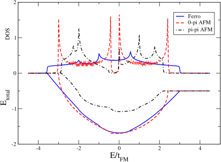
Figure 3: DOS for the three phases (top) and total energy of the three phases (bottom) plotted vs. energy/chemical potential

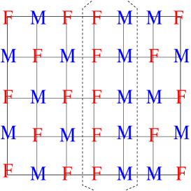
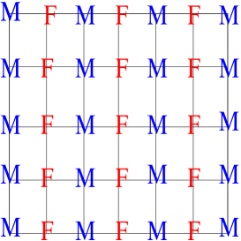
Figure 4: Top: A single domain line (combined Fe-Mo) antisite region in an otherwise ordered sample. F-srepresent the Iron atoms,and M-s the Molybdenum atoms. Bottom: Proliferation of such domains can result in the alternate Fe-Mo rich antisite structure depicted in Fig 2.

Interestingly, though, the remnant of the G-type antiferromagnet, most stable for large filling in the ordered phase mePinaki , is not found to be stabilized kinetically in any part of the filling in this phase segregated case.

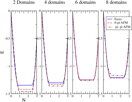
Figure 5: Energy vs filling for the three phases, compared for configurations with 2,4,6 and 8 domain Fe-Mo antisite defects.

In order to investigate how the kinetic energy driven stabilization behaviour changes from the ordered phase to the phase segregated phase with antisite defects, we have also considered intermediate phases with a combined Fe-Mo domain structure which is linear in the y direction (Fig 4). Using Exact Diagonalization calculations in real space, we have obtained the energies of the three phases, variationally, as a function of filling. Parameters used are $t_{FM}=1$,$t_{MM}=0.75$,$t_{FF}=0.5$ and $\Delta=0.5$. We considered intermediate configurations with 2,4, 6 and 8 domains in a $16\times 16$ lattice. This symbolizes propagation of the linear domains in the x direction. It is observed (Fig 5) that the antiferromagnetic phases slowly interchange their stability behaviour as the domains propagate through the lattice. There is a smooth transition from stabilization of the G-type phase in the low domain case to the stabilization of the A-type phase in the case with large number of domains. Thus a smooth interpolation is obtained from the ordered phase to the phase segregated phase, proving the scenario proposed earlier, and showing the continued kinetic energy induced stabilization of an antiferromagnetic metal phase for large filling; only the character of the antiferromagnetic phase changes. Although the G type phase is no longer stabilized kinetically, the superexchange, being nearest neighbour for the phase segregated case, and antiferromagnetic, can stabilize it, and bring its energy close to that of the A-type phase, even possibly surpassing it at some filling superex . Such a scenario can however, occur only for a small region of filling, as the G-type phase has the lowest bandwidth. Even then, the ground state continues to be an antiferromagnetic metal at high filling; either A type or G type, depending in the filling. It is interesting to note that even from kinetic energy considerations, the energy difference between the ferro and the ground state antiferromagnetic phase is much larger for the ordered case rather than in the phase segregated limit, as can be understood by comparing the figures for 2 domains and 8 domains. This can provide a plausible explanation to the signature of phase coexistence observed in the actual experiment using the phase segregated samples. Sugatapriv .

VI Summary and Outlook

We have considered the simplest model of phase segregation of B-site (Fe) and B$\prime$ site (Mo) in double perovskite Sr₂FeMoO₆, leading to antisite regions. Using variational methods, we have shown that an antiferromagnetic metal phase can still be stabilized in large regions of filling. The nature of the antiferromagnetic phase that is kinetically stabilized, is however, found to change as the system goes from ordered to phase segregated. Using extensive simulations in the intermediate phases involving antisite domains, we have verified that this transition is smooth, and the system remains an antiferromagnetic metal throughout for large regions of the filling, only the nature of the antiferromagnet changes from the ordered to the phase segregated limit.

VII Acknowledgment

The author gratefully acknowledges discussions with P. Majumdar, S.ray and T. Saha Dasgupta.

References

- (1) Y. Tomioka, T. Okuda, Y. Okimoto, R. Kumai, K.-I. Kobayashi, Y. Tokura, Phys. Rev. B 61, 422 (2000).
- (2) D.D. Sarma, P. Mahadevan, T. Saha Dasgupta, S. Ray, A. Kumar, Phys. Rev. Lett., 85, 2549 (2000)
- (3) K.-I. Kobayashi, T. Kimura, H. Sawada, K. Terakura, and Y. Tokura, Nature (London) 395, 677 (1998),
- (4) D.D. Sarma, Current Opinion in Solid State and Materials Science, 5, 261 (2001). .
- (5) B. Garcia Landa et al, Solid State Comm., 110, 435 (1999).
- (6) J. Navarro, L. Balcells, F. Sandiumenge, M. Bibes, A Roig, B Martinez and J. Fontcuberta, J. Phys.: Condens. Matter 13, 8481 (2001).
- (7) D. D. Sarma, S. Ray, K. Tanaka, M. Kobayashi, A. Fujimori, P. Sanyal, H.R. Krishnamurthy and C. Dasgupta, Phys. Rev. Lett., 98, 157205 (2007).
- (8) A. Kahoul, A. Azizi, S. Colis, D. Stoeffler, R. Moubah, G. Schmerber, C. Leuvrey, and A. Dinia, J. Appl. Phys. 104, 123903 (2008).
- (9) T. Saitoh, M. Nakatake, H. Nakajima, O. Morimoto, A. Kakizaki, Sh. Xu, Y. Moritomo, N. Hamada, Y. Aiura, Journal of Electron Spectroscopy and Related Phenomena 144-147, 601 (2005).
- (10) J. Navarro, C. Frontera, Ll. Balcells, B. Martnez, and J. Fontcuberta, Phys. Rev. B 64, 092411 (2001).
- (11) J. Navarro, J. Fontcuberta, M. Izquierdo, J. Avila, M.C. Asensio, Phys. Rev. B,70,054423 (2004).
- (12) Carlos Frontera, Diego Rubi, Jose Navarro, Jose Luis Garcia-Munoz, and Josep Fontcuberta, Phys. Rev. B 68, 012412 (2003).
- (13) Prabuddha Sanyal and Pinaki Majumdar, Phys. Rev. B, 80, 054411 (2009).
- (14) P. Sanyal, H.Das and T. Saha Dasgupta, Phys. Rev. B, 80, 224412 (2009).
- (15) S. Jana, C. Meneghini, P. Sanyal, S. Sarkar, T. Saha-Dasgupta, S. Ray, Phys. Rev. B, 86, 054433 (2012).
- (16) V. Singh and P.Majumdar, J. Phys. Condens. Matter, 26, 296001 (2014).
- (17) V.N. Singh, P. Majumdar, Europhys. Lett., 94, 47004 (2011).
- (18) A. Chattopadhyay and A. J. Millis, Phys. Rev. B 64, 024424 (2001).
- (19) O. Navarro, E. Carvajal, B. Aguilar, M. Avignon, Physica B 384, 110 (2006).
- (20) L. Brey, M. J. Caldern, S. Das Sarma and F. Guinea, Phys. Rev. B 74, 094429 (2006).
- (21) J.L.Alonso,L.A. Fernandez, F. Guinea, F. Lesmes, and V. Martin-Mayor, Phys. Rev. B, 67, 214423 (2003).
- (22) The nearest neighbour superexchange (active in antisite regions) affects the ferromagnetic phase and the A-type antiferromagnetic phase in the same way, and hence does not change their relative energies. Only the G type phase gets affected differently.