redrgb1,0,0 \definecolorgreenrgb0,1,0 \definecolorbluergb0,0,1
The Langevin Approach: a simple stochastic method for complex phenomena
Abstract
We describe a simple stochastic method, so-called Langevin approach, which enables one to extract evolution equations of stochastic variables from a set of measurements. Our method is parameter free and it is based on the nonlinear Langevin equation. Moreover, it can be applied not only to processes in time, but also to processes in scale, given that the data available shows ergodicity. This chapter introduces the mathematical foundations of this Langevin approach and describes how to implement it numerically. In addition, we present an application of the method to a turbulent velocity field measured in laboratory, retrieving the corresponding energy cascade and comparing with the results from a computer fluid dynamics (CFD) simulation of that experiment. Finally, we describe extensions of the method for time series reconstruction and applications to other fields such as finance, medicine, geophysics and renewable energies.
1 Introduction
”The present state of the universe is an effect of its past states and causes its future one”. Such a claim is a fundamental assumption in every physical approach to our surrounding nature and was mathematically defended for the first time two centuries ago, in 1814, by Simon Laplace. Laplace had a dream laplace , one where ”an intellect at a certain moment would know all forces that set nature in motion, and all positions of all items of which nature is composed, […] vast enough to submit these data to analysis […], to embrace in a single formula [all movements of the universe]”. Why was this a dream? Because there are strong arguments against it, such as thermodynamic irreversibility, quantic indeterminacy and nonlinear sensitivity to initial states. But there is also a practical reason: such a high-dimensional problem, due to its huge number of variables, would only be computable if one would take as model of reality the reality itself, an approach which is pointless. To model reality one needs simplifications and stochastic methods enables one to simplify reality in several adequate ways. In this chapter we describe one of such ways, which, in the last fifteen years, has been successfully applied in several fields physrepreview .
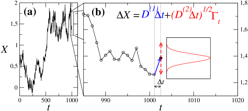
As an illustration we address the problem of turbulence, one of the central open problems in physics turbulencebook . A turbulent fluid is governed by the so-called Navier-Stokes equations which cannot be approached analytically in all their detail. Therefore one handles Navier-Stokes equations numerically, developing discretization schemes which yield the solution of one specific problem. Such discretization in space and time corresponds in general to high-dimensional problems which, in the limit of infinitely small discrete elements, leads to infinite many degrees of freedom. Such numerical approaches to the equations governing turbulence enabled rather successful insight and modeling approaches for fundamental physics and engineering applications turbulencebook .
However, the Navier-Stokes equations, which are purely deterministic, could be substituted by a stochastic approach, using only a few – the essential – variables, say () and incorporating the rest of the degrees of freedom in a “stochastic bag”. In this way one arrives to evolution equations of the type:
| (1) |
where function is a deterministic function depending on each variable and function depends not only on variables but also on stochastic forces (). For , equation (1) reduces to a deterministic dynamical system and for one can take it as a deterministic dynamical system subjected to small noise of constant amplitude nontimeseries .
In general however, not only function cannot be neglected but it possesses a much more complicated (nonlinear) dependence on the accounted variables. Such functional dependence of is important, for instance when one intends to describe physical features of a process underlying a set of data or when aiming at predicting or reconstructing a set of observations.
Having properly defined an equation such as equation (1), it should be possible to reconstruct series of values of one variable, say in a statistical sense, i.e. it should be possible to derive the conditional probability:
| (2) |
for each set of values with . See sketch in Fig. 1.
In this chapter we will describe in detail how to derive an evolution equation such as equation (1) from a set of measurements. Our method, so-called Langevin approach, is fully introduced in Sec. 2. In in Sec. 3 the Langevin approach is applied to turbulence by using the data gained from an experimental study in Sec. 3.1. Furthermore, the Langevin approach is applied to a numerical simulation of the experimental study in Sec. 3.2. A comparative analysis, discussing the results obtained in the experiments and simulations is given in Sec. 3.3. Section 4 concludes this chapter, discussing briefly recent trends in the Langevin approach and other possible fields and topics where it can be successfully applied.
2 The Langevin approach
To introduce the Langevin approach, we first explain in Sec. 2.1 what processes in scale111In statistics such processes are also known as branching processes. are and relate them with the usual processes in time. In Sec. 2.2, the necessary conditions under which the Langevin approach is applied are given together with a brief description of how to verify these conditions in empirical and simulated data. Section 2.3 describes the derivation of the deterministic and stochastic contributions with a given set of measurements taken from a process in scale. Finally, in Sec. 2.4 we derive the stochastic evolution equation describing a process in scale. A particular example is described, namely the ”Brownian motion” in scale, using the Galton box as an illustration, which complements the usual Brownian motion described by Einstein einstein1905 and Langevin Langevin1908 .
2.1 Processes in scale
There is a famous poem by Richardson turbulencebook about turbulence which summarizes his important paper from 1920 richardson : ”a turbulent fluid is composed by a few big eddies that decay into smaller eddies, these ones into even smaller eddies, and so on to viscosity”. The energy that feeds the turbulent fluid enters the system on large scales – through the largest eddies – and travels towards smaller and smaller scales up to a minimum scale where it leaves the system by means of dissipation. In each of these steps the energy of the larger eddy is randomly distributed between the smaller “child” eddies. Such a pictorial view of turbulent energy traveling through a hierarchical succession of length scales leads to the concept of the turbulent energy cascade evolving in the spatial length scale as the independent variable.
One may ask if it would be possible to extract such energy cascade from empirical data, e.g. from a set of velocity measurements at one specific point of the fluid. In the following we show that indeed it is possible friedrich1997 ; renner2001 ; physrepreview . Describing how a property behaves across an ordered series of different spatial scales is analogous to the more common description of the evolution of a property in time, with the important difference that instead of the time-propagator in equation (2) one has now a “scale-propagator”.
Assuming that one has a non-negligible stochastic contribution, the aim is to derive an equation analogous to equation (1) where the spatial scale plays the role of time . Since the independent variable accounts for the size of some structure, like an eddy, we choose for the dependent variable the difference of an observable at two distinct positions, separated by , namely the increment
| (3) |
with being a specific location in the system. Thus, the scale-propagator describes how this increment – or difference – changes when the distance increases or decreases as follows:
| (4) |
Four important remarks are due here. First, the scale increment in equation (4) can in general be positive or negative. In fact, as we will see in the next sections, the energy in turbulence flows from the largest scales, of the size of the system itself, toward the smallest scale at which dissipation takes place. Therefore, in turbulence one considers a scale-propagator as in (4) with .
Second, one should define a proper metric for the scale . Is the spatial distance the best choice? Or is there a more appropriate functional of spatial distances? A process in time evolves according to an iteration from to . The same should occur for processes in scale. However, when ”iterating” from one scale to the ”next”, one iterates in a multiplicative way, i.e., from one scale to the next one one multiplies the previous scale by some constant , yielding a succession of scales . A suitable choice of an additive scale, similar to the additive time iteration, is the logarithmic scale , since in this case one has . This logarithm scale is of importance to understand the concept of self-similarity, which is closely related to processes in scale. Self-similarity is the property that a phenomenon may manifest, by showing invariance under multiplicative changes of scale, as observed in turbulent flows. Indeed, following Richardson’s poem, eddies are self-similar objects, since multiplying or dividing their size by a proper scaling factor we obtain an eddy again. With the logarithmic scale we “convert” the multiplicative changes into additive ones.
Third, when analyzing processes in scale, ideally one would consider a field of measurements taken simultaneously within a spatially extended region. What one typically has, contrastingly, is a set of measurements in time taken at a particular location. To extract processes in scale from single time series, one requires the property being measured to be ergodic: the system should display the same behaviour averaged either over time or over the space of all the system’s states. In the particular case of a turbulent fluid, ergodicity reduces to the so-called Taylor hypothesis turbulencebook .
Fourth, while the derivation of a propagator in scale may be helpful for uncovering phenomena such as the energy cascade in turbulence, one may also aim to bridge from the derived propagator in scale to a propagator in time which would enable time-series reconstruction. As shown in previous works Nawroth2010 , our Langevin approach enables such bridging from scale to time.
Henceforth, we will consider a process in scale, i.e. a succession of increments of a measurable property , with:
| (5) |
taking values from (largest scale ) to at the smallest scale . Notice that, and therefore, for one arrives again at a positive scale increment.
2.2 Necessary conditions: stationarity and the Markov property
To apply our method, two important features must be met. First, the set of measures from which one extracts the succession of increments in scale must be a stationary process. Second, the process in scale must be Markovian.
For the process to be stationary, the corresponding conditional probability in equation (2) should be invariant under a translation in time, , . Numerically such property cannot be tested in sets of measurements. As an alternative, one usually divides the set of measurements in subsets of data points and computes the first four centred moments. In case the centred moments do not vary significantly from one subset to the next one, the set of measurements is taken as stationary.
The Markov condition of the scale process reads vankampen :
| (6) |
Notice that, an important consequence of the Markov condition is that any -point statistics on can be extracted from the two-point statistics risken on the increments, , i.e. three-point statistics on . The two-point joint distribution of the increments contains all the information of the scale process.
Equation (6) tells us that, any conditional probability distribution from the process conditioned to an arbitrarily large number of previous observations equals the condition probability conditioned to the single previous observation solely. Again, such condition is not possible to ascertain in all its mathematical detail. A weaker version of equation (6) suitable for numerical implementation is:
| (7) |
Both conditions in equations (6) and (7) are equivalent under the physically reasonable assumption that the dependency of the future state on previous states decreases monotonically with the time-lag. The equality in equation (7) can be qualitatively verified by plotting contour plots in the range of observed values for and , and fixing . It can also be quantitatively tested through the Wilcoxon test wilcoxon , -test, or by computing a Kullback-Leibler distance between both conditional distributions statisticalbook .
2.3 The Fokker-Planck equation for increments
Once the stationarity of our measures as well as the Markov condition for their increments are fulfilled, we are able to determine multipoint statistics for our increments. Since the process is Markovian in scale, it can be easily proven that for any integer one has:
| (8) | |||||
| , | (10) |
and
| (11) |
for all . Thus, all information of our process is incorporated in the two-point statistics of the increments.
It is known that risken , the conditional probability distributions obeys the so-called Kramers-Moyal (KM) equation:
| (12) |
with functions , so-called KM coefficients, being defined through conditional moments in the limit of small scale increments, namely:
| (13a) | |||||
| (13b) | |||||
Notice that, from equation (13a), one can see that mathematically each KM coefficient of order , apart a multiplicative constant , is the derivative of the conditional moment of the same order .
Numerically, there are two ways for deriving KM coefficients. One is by computing the conditional moments for a range of observed values of and , which is divided in a certain number of bins, and repeating the computation for several values of . In the case where the conditional moments depend linearly on , at least for the lower range of values, the KM coefficients are taken as the slope of the linear interpolation of the corresponding conditional moment in that range of values. In case such linear dependency is not observed, a second procedure is possible: one computes at once the entire fraction within the limit in equation (13a) again for a range of observed values of and , divided in a proper number of bins, but this time one takes the range of smallest values of and through a linear interpolates infers the projection in the plane .
The error for are just given by the linear interpolation of the corresponding conditional moments as functions of . The errors of each value , necessary for computing the errors of the linear interpolation, are given by lind2010 :
| (14) |
The KM equation (12) also holds for the single probability distribution, since multiplying both sides by and integrating in yields the same equation for .
An important simplification in equation (12) follows if the fourth KM coefficient vanishes or is sufficiently small compared to the first two KM coefficients. Such simplification is based on Pawula’s Theorem which states that if then all coefficients in equation (12) are identically zero except the first two. Consequently the Kramers-Moyal equation reduces to the so-called Fokker-Planck equation:
| (15) |
For such differential equation of the single probability function one can derive differential equations for the structure functions of the increments renner2001 . Uncertainties in equation (13a) can be overcome, namely when estimating the limit, by considering a subsequent optimization of and . This optimization procedure is based in a cost function derived from the conditional probability density functions, which are deduced from both the experimental data and from Kramers-Moyal coefficients directly Kleinhans ; Nawroth .
2.4 Langevin processes in scale
The Fokker-Planck equation (15) above describes the evolution of the conditional probability density function for a process in scale which can be generated by a Langevin equation of the form:
| (16) |
where is a -correlated noise (in scale ) with and .
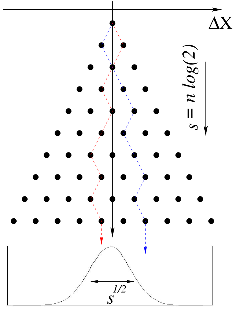
To illustrate the Langevin process in scale described by equation (16), we consider the particular case of and constant , reducing the general Langevin equation to the particular case of Brownian motion ”in scale”.
What is the Brownian motion in scale? Though more abstract than the usual Brownian motion Langevin1908 , Brownian motion in scale can be illustrated by a Galton Box Galton , as sketched in figure 2. The Galton box is an apparatus consisting of a vertical board with interleaved rows of pins, typically with a constant distance between neighbouring pins. Balls are dropped from the top, and each time they hit a pin, they bounce, left or right, downwards. At the bottom, balls are collected in several columns separated from each other.
In a Galton box, the horizontal rows of pins represent the succession of scales, , with a constant distance between adjacent rows, representing the scale increment . From one scale to the next one the possible ways a ball can bounce doubles. Since is in fact a logarithmic scale of , , and therefore scales linearly with the vertical distance to the starting point.
As for the horizontal distance from the centred vertical line, it represents the increments . We recall that for processes in scale one has a scale playing the role of time and one has increments instead of single values of the observable . Thus, similarly to the solution of the original Langevin equation for Brownian motion, in this case one also obtains a Gaussian distribution of increment values centred at and with a variance proportional to . Note that the normal approximation of this binomial distribution is .
Such illustration of a process in scale is a very simple one. To properly imagine a picture of general scale processes in turbulence two important differences must be considered. First, the energy (i.e. velocity increments) flow from the largest to the smallest scales, which is opposite to the illustration with the Galton box. Second, the KM coefficients for the Galton box are those of the simplest situation that we named as Brownian motion in scale, due to its straightforward parallel with usual Brownian motion. Here the KM coefficients do not depend on scale . In turbulence, as we will see, not only the dependency on the increments is more complicated, but there is an important dependence on the scale .
3 Applying the Langevin approach to turbulence
3.1 The Langevin approach in laboratory turbulence
The experiments were conducted in a closed loop wind tunnel with test section dimensions of 200 cm x 25 cm x 25 cm (length x width x height) at the University of Oldenburg. The wind tunnel has a background turbulence intensity of approximately for m/s. The inlet velocity was set to 10 m/s, which corresponds to a Reynolds number related to the biggest grid bar length of about , where is the kinematic viscosity. Constant temperature anemometry measurements of the velocity were performed using (Dantec 55P01 platinum-plated tungsten wire) single-hot-wire with a wire sensing length of about mm and a diameter of which corresponds to a length-to-diameter ratio of . A StreamLine measurement system by Dantec in combination with CTA Modules 90C10 and the StreamWare version 3.50.0.9 was used for the measurements. The hot-wire was calibrated with Dantec Dynamics Hot-Wire Calibrator. The overheat ratio was set to 0.8. In the streamwise direction, measurements were performed on the centerline in the range between 5 cm 176 cm distance to the grid. The data was sampled with kHz with a NI PXI 1042 AD-converter and 3.6 million samples were collected per measurement point, representing 60 seconds of measurements data. To satisfy the Nyquist condition, the data were low-pass filtered at frequency kHz.
For the present work, a fractal grid was placed at the inlet of the wind tunnel, see figure 3. In general, fractal grids are constructed from a multiscale collection of obstacles which are based on a single pattern which is repeated in increasingly numerous copies with different scales. The pattern our fractal grid is based on is a square shape with fractal iterations. The fractal iterations parameter is the number the square shape is repeated at different scales. At each iteration , the number of squares is four times higher than in the iteration . Each scale iteration is defined by a length and a thickness of the squares bars constituting the grid. The thickness of the square bars in the streamwise direction is constant. The dimensions of the square patterns are related by the ratio of the length of subsequent iterations and by the ratio of the thickness of subsequent iterations ; respectively. The geometry of the fractal grid we used (also called the space filling fractal grid Hurst07 ) is completely characterized by two further parameters namely the ratio of the length of the first iteration to the last one and the ratio of the thickness of the first iteration to the last one .
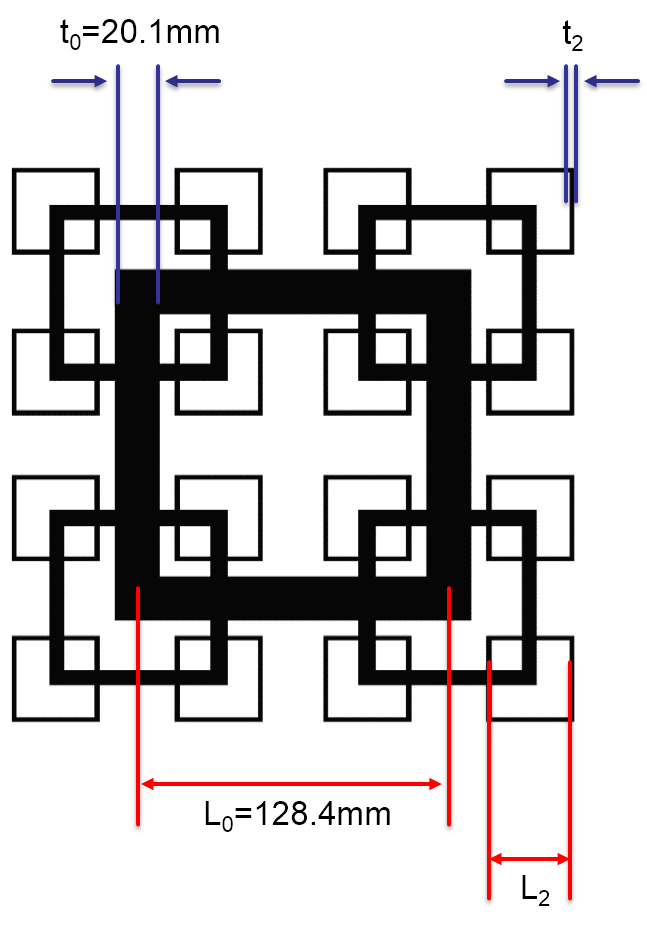
Contrary to classical grids, fractal grids do not have a well-defined mesh size . However, an equivalent effective mesh size was defined in Hurst07 . A complete quantitative description of the N3 fractal grid we used in this study is reported in table 1.
| 3 | 36.4 |
|---|
3.2 The Langevin approach in simulated turbulence
The flow over a fractal grid is described by the three dimensional, incompressible Navier-Stokes equations. The equations are discretized and solved using a turbulence model. In this investigation, the Delayed Detached Eddy Simulation (DDES) Spalart_Strelets_1997 with a Spalart-Allmaras background turbulence model Spalart_Allmaras_1994 , commonly referred to as SA-DDES is used. DDES is a hybrid method stemming from the Detached Eddy Simulation method (DES) Spalart_Strelets_1997 , which involves the use of Reynolds Averaged Navier-Stokes Simulation (RANS) at the wall and Large Eddy Simulation (LES) away from it. This method combines the simplicity of the RANS formulation and the accuracy of LES, with the advantage of being less expensive, in terms of computational time, when compared with pure LES. DDES is an improvement of the original DES formulation, where the so called ”modelled stress depletion” (or MSD), is treated Menter_2004 ; Spalart_2006 .
The numerical simulation was set up analogous to the experiments in order to compare the results in a consistent manner. The open source code OpenFOAM OpenFOAM:website was used to solve the incompressible Navier-Stokes equations. OpenFOAM is based on the finite volume method, and it consists of a collection of libraries written in C++, which can be used to simulate a large class of flow problems. For more information about the available solvers and turbulence models, refer to the official documentation OpenFOAM:website . The solver used in this investigation is the transient solver pimpleFoam, which is a merging between the PISO (Pressure implicit with splitting of operator) and SIMPLE (Semi-Implicit Method for Pressure Linked Equation) algorithms. A second order central-differencing scheme is used for spatial discretization, and a backward, second-order time advancing schemes was used. The solver is parallelized using the Message-Passing Interface (MPI), which is necessary for problems of this size.
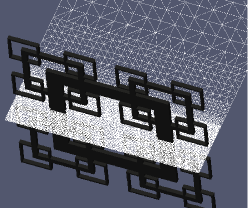
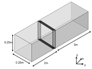
The numerical mesh was generated using the built-in OpenFOAM meshing tools blockMesh and snappyHexMesh OpenFOAM:website . As a result, an unstructured mesh of 24 million cells is obtained, where regions of interest in the wake are refined, as shown in Fig. 4. The fractal grid is simulated in a domain with similar dimensions as the real wind tunnel. The domain begins 2 m upstream of the fractal grid and covers a distance of 2 m downstream (see Fig. 5). The flow-parallel boundaries are treated as frictionless walls, where the slip boundary condition was applied for all flow variables. At the inflow boundary, Neumann boundary condition was used for the pressure, and Dirichlet condition for the velocity. At the outflow boundary, the pressure was set to be equal to the static pressure and a Neumann boundary condition was used for the velocity. On the fractal grid, a wall function is used for the modified viscosity , with the size of the first cell of the mesh in terms of the dimensionless wall distance is whiteCFD . For each simulation, 480 processors were used, and for each time step 4.5 of data was collected for post-processing. The data sampling frequency was 60 , chosen to match the experimental one. It took approximatively 72 hours to simulate one second of data and a total of 20 seconds of numerical data were collected. The data was collected in the same positions as for the experimental study. The numerical simulations were conducted on the computer cluster of the ForWind Group FLOW01:website .
3.3 Comparative analysis
| KM coeff. | Data | ||||
|---|---|---|---|---|---|
| exp. | |||||
| Sim. | |||||
| Exp. | |||||
| Sim. | |||||
| Exp. | |||||
| Sim. |
(a)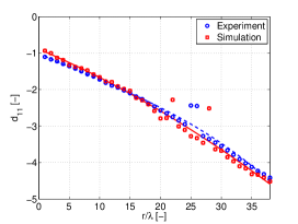 (b)
(b)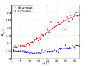 (c)
(c)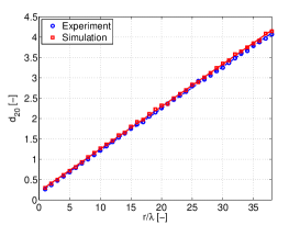
We estimate the Kramers-Moyal coefficients for the experimental and simulated data. The coefficients are commonly parametrized as follows:
| (17) | |||||
| (18) | |||||
| (19) |
The results of in terms of , , and are shown in table 2, for the downstream position . Note that the coefficients strongly depend on the downstream position . We present and discuss all scales in units of Taylors microscale .
Figure 6 presents Kramers-Moyal coefficients in terms of , and vs. the scale . The coefficient are calculated within the inertial range. We chose this range, because the DDES simulations treat flow structures of this size as universal and simplify the turbulent flow properties by means of a sub-grid model, which is in this case the Spalart-Allmaras model. Therefore, a validation with the experimental data within the inertial range is of particular interest. Common limits of this region are (small scale) and the integral length scale (large scale).
The development of the drift term within the inertial range is shown in figure 6(a). Comparing the experimental and the simulated data no significant differences can be observed. Both curves indicate a stronger drift term with increasing scale, as usual for turbulent flows. The four outliers are most likely due to the optimization procedure. Rarely, local minimum are found instate of the global.
The development of the diffusion term within the inertial range is shown in figure 6(b) and (c). Figure 6(b) shows the curvature of the diffusion term , a very small and sensitive term. Here the experimental and the simulated data differ in their development. At large scales the curvature differ significantly (). At small scales the developments draw near, but do not converge. The magnitude of is common, and shows why some studies neglect . Figure 6(c) presents the diffusion term offset within the inertial range. Such as the drift term, no essential differences between the experimental and the simulated data can be observed. The linear increasing of the offset is typical for the inertial range, it indicates the growth of the increments (velocity difference) or vortices, respectively, with scale, cf. equation (16).
4 Discussion and Conclusions
In this chapter we described the so-called Langevin approach, a stochastic method that enables deriving evolution equations of stochastic observables, providing important physical insight about the underlying system.
The method was applied to the problem of turbulence, addressed experimentally and by means of simulations by extracting the velocity increment time series, one recorded in a wind tunnel experiment and one simulated by a delayed detached large eddy simulation (DDES). For each case we extracted the functions defining the stochastic evolution equation, the so-called Kramers-Moyal coefficients, and parametrized them through polynomials of the scale.
The results show on the one hand good consistency in the two dominating terms, namely the linear term of the first KM coefficient (drift) and the independent term of the second KM coefficient (diffusion). Other terms, such as the quadratic term for the diffusion, may present deviations that appeal for further investigation, which will carried out for a forthcoming study focusing on this specific experiment.
Concerning the Langevin approach as a stochastic method on its own, three points are worth of mention. First, the method can also be applied to the usual processes in time physrepreview . For that, one should simply interchange scale and increments in equations (12) and (16) by time and observable values respectively.
Second, while the method implies the fulfilment of two important conditions, namely stationarity and markovianity (see Sec. 2.2), the method can still be adapted to a more general situation where one or both this conditions are dropped. In case the data series is not stationary, the Langevin approach can be applied to time-windows within which the series can be taken as stationary silvio . As a result, one derives a set of KM coefficients as function of time, one for each time-window. In the case the data series is not Markovian, for instance due to measurement (additive) noise an extension is still possible lind2010 ; boettcher2006 .
Finally, the Langevin approach can be applied to a broad panoply of different situations in topics ranging technical applications to biological, geophysical and financial systems, e.g. electric circuits, wind energy converters, traffic flow, cosmic microwave background radiation, granular flows, porous media, heart rhythms, brain diseases such as Parkinson and epilepsy, meteorological data, seismic time series, nanocrystalline thin films and biological macromolecules. For a review on these topics see Ref. physrepreview .
5 Acknowledgement
We gratefully acknowledge the computer time provided by the Facility for Large-Scale Computations in Wind Energy Research (FLOW) of the university of Oldenburg. WM thanks the German Bundesministerium für Umwelt, Naturschutz und Reaktorsicherheit (BMU), which financed this project. PGL thanks German Federal Ministry of Economic Affairs and Energy (BMWi) as part of the research project “OWEA Loads” under grant number 0325577B.
References
- (1) D. Hurst, J.V.: Scalings and decay of fractal-generated turbulence. Physics of Fluids 19, 035,103 (2007)
- (2) Einstein, A.: über die von der molekularkinetischen theorie der wärme geforderte bewegung von in ruhenden flüssigkeiten suspendierten teilchen. Annalen der Physik 17, 549–560 (1905)
- (3) F.Boettcher, J.Peinke, D.Kleinhans, R.Friedrich, P.G.Lind, M.Haase: Reconstruction of complex dynamical systems affected by strong measurement noise. Phys. Rev. Lett. 97, 090,603 (2006)
- (4) Flow01: Facility for large-scale computations in wind energy research (2013). http://www.fk5.uni-oldenburg.de/57249.html
- (5) Friedrich, R., Peinke, J.: Description of a turbulent cascade by a fokker-planck equation. Phys. Rev. Lett. 78, 863 (1997)
- (6) Friedrich, R., Peinke, J., Sahimi, M., Tabar, M.: Approaching complexity by stochastic methods: From biological systems to turbulence. Phys. Rep. 506, 87 (2011)
- (7) Galton, F.: Natural Inheritance. Macmillan (1894)
- (8) van Kampen, N.: Stochastic Processes in Physics and Chemistry. North-Holland (1999)
- (9) Kleinhans, D., Friedrich, R., Nawroth, A.P., Peinke, J.: An iterative procedure for the estimation of drift and diffusion coefficients of langevin processes. Phys. Letters A 346, 42–46 (2005)
- (10) Langevin, P.: On the theory of brownian motion. C. R. Acad. Sci. 146, 530–533 (1908)
- (11) Laplace, P.: A Philosophical Essay on Probabilities. Dover Publications 1951 (1814)
- (12) Lind, P., Haase, M., Boettcher, F., Peinke, J., Kleinhans, D., Friedrich, R.: Extracting strong measurement noise from stochastic series: applications to empirical data. Phys. Rev. E 81, 041,125 (2010)
- (13) Lowry, R.: Concepts and Applications of Inferential Statistics. available at http://vassarstats.net/textbook/ (2011)
- (14) Menter, F.R., Kuntz, M.: The Aerodynamics of Heavy Vehicles: Trucks, Buses, and Trains. In: Volume 19 of Lecture notes in Applied and Computational Mechanics (2004)
- (15) Nawroth, A.P., Friedrich, R., Peinke, P.: Multi-scale description and prediction of financial time series. New Journal of Physics 12, 083,021 (2010)
- (16) Nawroth, A.P., Peinke, J., Kleinhans, D., Friedrich, R.: Improved estimation of fokker-planck equations through optimisation. Phys. Rev. E. 76(056102) (2007)
- (17) OpenFOAM: The open source computational fluid dynamics toolbox (2013). http://www.openfoam.com/
- (18) Pope, S.: Turbulence Flows. Cambridge Univ. Press (2000)
- (19) Renner, C., Peinke, J., Friedrich, R.: Experimental indications for markov properties of small-scale turbulence. J. Fluid Mech. 433, 383–409 (2001)
- (20) Richardson, L.F.: The supply of energy from and to atmospheric eddies. Proc.nR. Soc. Lond. A 97, 354–376 (1920)
- (21) Risken, H.: The Fokker-Planck Equation. Springer, Heidelberg (1984)
- (22) S.Camargo, Queirós, S., C.Anteneodo: Nonparametric segmentation of nonstationary time series. Phys. Rev. E 84, 046,702 (2006)
- (23) Schreiber, T., Kantz, H.: Nonlinear Time-series Analysis. Cambridge Univ. Press, Cambridge (1999)
- (24) Spalart, P., Deck, S., Shur, M., Squires, K., Strelets, M., Travin, A.: A new version of detached-eddy simulation, resistant to ambiguous grid densities. Theoretical and Computational Fluid Dynamics 20(3), 181–195 (2006)
- (25) Spalart, P.R., Allmara, S.R.: A One-Equation Turbulence Model for Aerodynamic Flows. La Recherche Aerospatiale 1, 5–21 (1994)
- (26) Spalart, P.R., Strelets, M., Allmara, S.R.: Comments on the feasibility of LES for wings, and on a hybrid RANS/LES approach. Advances in DES/LES 1, 137–147 (1997)
- (27) White, F.: Fluid Mechanics. McGraw-Hill Higher Education 1998 (1998)
- (28) Wilcoxon, F.: Individual comparisons by ranking methods. Biometrics Bulletin 1, 80–83 (1945)