To understand the rare decay $B_{s}\to\pi^{+}\pi^{-}\ell^{+}\ell^{-}$

Abstract

Motivated by the LHCb measurement, we analyze the $B_{s}\to\pi^{+}\pi^{-}\ell^{+}\ell^{-}$ decay in the kinematics region where the pion pairs have invariant mass in the range $0.5$-$1.3$ GeV and muon pairs do not originate from a resonance. The scalar $\pi^{+}\pi^{-}$ form factor induced by the strange $\bar{s}s$ current is predicted by the unitarized approach rooted in the chiral perturbation theory. Using the two-hadron light-cone distribution amplitude, we then can derive the $B_{s}\to\pi^{+}\pi^{-}$ transition form factor in the light-cone sum rules approach. Merging these quantities, we present our results for differential decay width which can generally agree with the experimental data. More accurate measurements at the LHC and KEKB in future are helpful to validate our formalism and determine the inputs in this approach.

Very recently, the LHCb has performed an analysis of rare $B_{s}$ decays into the $\pi^{+}\pi^{-}\mu^{+}\mu^{-}$ final state Aaij:2014lba and the branching fraction is measured as

$${\cal B}(B_{s}\to\pi^{+}\pi^{-}\mu^{+}\mu^{-})=(8.6\pm 1.5\pm 0.7\pm 0.7)\times 10^{-8},$$ (1)

where the first two errors are statistical, and systematic respectively. The third error is due to uncertainties on the normalization, i.e. the branching fraction of the $B^{0}\to J/\psi(\to\mu^{+}\mu^{-})K^{*}(\to K^{+}\pi^{-})$. The branching fraction for $B_{s}\to f_{0}(980)\mu^{+}\mu^{-}$ Aaij:2014lba is determined as:

$${\cal B}(B_{s}\to f_{0}(980)(\to\pi^{+}\pi^{-})\mu^{+}\mu^{-})=(8.3\pm 1.7)\times 10^{-8},$$ (2)

which lies in the vicinity of the total branching fraction in Eq. (1). Despite the errors, the closeness of the two branching fractions and the differential distribution as shown later in Fig. (4b) may indicate the dominance of the $f_{0}(980)$ contributions in the $B_{s}\to\pi^{+}\pi^{-}\mu^{+}\mu^{-}$.

The $B_{s}\to\pi^{+}\pi^{-}\mu^{+}\mu^{-}$ is a four-body process. Its decay amplitude shows two distinctive features. On the one side, the $\pi^{+}\pi^{-}$ final state interaction is constrained by unitarity and analyticity. On the other side, the $b$ mass scale is much higher than the hadronic scale $\Lambda_{\rm QCD}$, which allows an expansion of the hard-scattering kernels in terms of the strong coupling constant $\alpha_{s}$ and the dimensionless power-scaling parameter $\Lambda_{\rm QCD}/m_{b}$. In Refs. Meissner:2013hya ; Meissner:2013pba ; Doring:2013wka , we have developed a formalism that makes use of these two advantages. This approach was also pioneered in Ref. Gardner:2001gc ; Maul:2001zn , and see also Refs. Chen:2002th ; Chen:2004az ; Wang:2014ira ; Wang:2014qya for applications to charmless three-body $B$ decays. In doing this, the new formalism can simultaneously merge the perturbation theory at the $m_{b}$ scale and the low-energy effective theory based on the chiral symmetry to describe the S-wave $\pi\pi$ scattering. The aim of this work is to further examine this formalism by confronting this theoretical framework with the recent data on $B_{s}\to\pi^{+}\pi^{-}\mu^{+}\mu^{-}$. An independent analysis that is based on the perturbative QCD approach is also under progress Wang:2015uea

We start with the differential decay width for $B_{s}\to\pi^{+}\pi^{-}\ell^{+}\ell^{-}$. The effective Hamiltonian for the transition $b\to s\ell^{+}\ell^{-}$

$${\cal H}_{\rm{eff}}=-\frac{G_{F}}{\sqrt{2}}V_{tb}V^{*}_{ts}\sum_{i=1}^{10}C_{i}(\mu)O_{i}(\mu)$$

involves various four-quark and the magnetic penguin operators $O_{i}$. the $C_{i}(\mu)$ are the corresponding Wilson coefficients for these local operators $O_{i}$. $G_{F}$ is the Fermi constant, and $V_{tb}=0.99914\pm 0.00005$ and $V_{ts}=-0.0405^{+0.011}_{-0.012}$ Agashe:2014kda are the CKM matrix elements. The $b$ and $s$ quark masses are $m_{b}=(4.66\pm 0.03)$GeV and $m_{s}=(0.095\pm 0.005)$GeV Agashe:2014kda . The $b\to sl^{+}l^{-}$ transition has the decay amplitude

$$i{\cal M}(b\to s\ell^{+}\ell^{-}) = iN_{1}\times\bigg{\{}({C_{9}+C_{10}})[\bar{s}b]_{V-A}[\bar{\ell}\ell]_{V+A}+({C_{9}-C_{10}})[\bar{s}b]_{V-A}[\bar{\ell}\ell]_{V-A}$$ (3)

$$+4C_{7L}m_{b}[\bar{s}i\sigma_{\mu\nu}(1+\gamma_{5})b]\frac{q^{\mu}}{q^{2}}\times[\bar{\ell}\gamma^{\nu}\ell]+4C_{7R}m_{b}[\bar{s}i\sigma_{\mu\nu}(1-\gamma_{5})b]\frac{q^{\mu}}{q^{2}}\times[\bar{\ell}\gamma^{\nu}\ell]\bigg{\}},$$

where $C_{7L}=C_{7}$ and $C_{7R}=C_{7L}{m_{s}}/{m_{b}}$, and

$$N_{1}=\frac{G_{F}}{4\sqrt{2}}\frac{\alpha_{\rm em}}{\pi}V_{tb}V_{ts}^{*}.$$ (4)

The $B\to M_{1}M_{2}\ell^{+}\ell^{-}$ is a four-body decay mode, whose decay amplitude can be obtained by sandwiching Eq. (3) between the initial and final hadronic states. The spinor product $[\bar{s}b]$ will be replaced by corresponding hadronic matrix elements. A general differential decay width for $B\to M_{1}M_{2}\ell^{+}\ell^{-}$ with various partial wave contributions has been derived using the helicity amplitude in Ref. Lu:2011jm . In the $B_{s}\to\pi^{+}\pi^{-}\mu^{+}\mu^{-}$ case, the S-wave contribution will dominate and thus the angular distribution is derived as

$$\frac{d^{3}\Gamma}{dm_{\pi\pi}^{2}dq^{2}d\cos\theta_{l}} = \frac{3}{8}\Big{[}J_{1}^{c}+J_{2}^{c}\cos(2\theta_{l})\Big{]},$$ (5)

where $\theta_{l}$ is the polar angle between the $\mu^{-}$ and the $B_{s}$ moving direction in the lepton pair rest frame. The angular coefficients are given by

$$J_{1}^{c} = \bigg{\{}|{\cal A}^{0}_{L0}|^{2}+|{\cal A}^{0}_{R0}|^{2}+8\hat{m}_{l}^{2}|{\cal A}^{0}_{L0}{\cal A}^{0*}_{R0}|\cos(\delta_{L0}^{0}-\delta_{R0}^{0})+4\hat{m}_{l}^{2}|{\cal A}_{t}^{0}|^{2}\bigg{\}},$$ (6)

$$J_{2}^{c} = -\beta_{l}^{2}\bigg{\{}|{\cal A}^{0}_{L0}|^{2}+|{\cal A}^{0}_{R0}|^{2}\bigg{\}}.$$ (7)

In the above equations, $\beta_{\ell}=\sqrt{1-4m_{\ell}^{2}/q^{2}}$, and $\hat{m}_{\ell}=m_{\ell}/\sqrt{q^{2}}$. The helicity amplitude is

$${\cal A}_{L/R,0}^{0} = \sqrt{N_{2}}i\frac{1}{m_{\pi\pi}}\Bigg{[}(C_{9}\mp C_{10})\frac{\sqrt{\lambda}}{\sqrt{q^{2}}}{\cal F}_{1}(q^{2})+2(C_{7L}-C_{7R})\frac{\sqrt{\lambda}m_{b}}{\sqrt{q^{2}}(m_{B}+m_{\pi\pi})}{\cal F}_{T}(q^{2})\Bigg{]},$$

$${\cal A}_{L/R,t}^{0} = \sqrt{N_{2}}i\frac{1}{m_{\pi\pi}}\Bigg{[}(C_{9}\mp C_{10})\frac{m_{B}^{2}-m_{\pi\pi}^{2}}{\sqrt{q^{2}}}{\cal F}_{0}(q^{2})\Bigg{]},$$ (8)

where

$$N_{2}=\frac{1}{16\pi^{2}}N_{1}N_{\pi\pi}\sqrt{1-4m_{\pi}^{2}/m_{\pi\pi}^{2}},\ N_{\pi\pi}=\sqrt{\frac{8}{3}}\frac{\sqrt{\lambda}{q^{2}}\beta_{\ell}}{256\pi^{3}m_{B}^{3}}.$$ (9)

Here the script $t$ denotes the time-like component of a virtual state decays into a lepton pair. The function $\lambda$ is related to the magnitude of the $\pi^{+}\pi^{-}$ momentum in $B_{s}$ meson rest frame: $\lambda\equiv\lambda(m^{2}_{B_{s}},m^{2}_{\pi^{+}\pi^{-}},q^{2})$, and $\lambda(a^{2},b^{2},c^{2})=(a^{2}-b^{2}-c^{2})^{2}-4b^{2}c^{2}$. The combination of the time-like decay amplitude is introduced in the differential distribution

$${\cal A}_{t}^{0} = {\cal A}_{R,t}^{0}-{\cal A}_{L,t}^{0}=2\sqrt{N_{2}}C_{10}i\frac{1}{m_{\pi\pi}}\Bigg{[}\frac{m_{B_{s}}^{2}-m_{\pi\pi}^{2}}{\sqrt{q^{2}}}{\cal F}_{0}(q^{2})\Bigg{]}.$$ (10)

The $B_{s}\to\pi\pi$ form factors used in Eq. (8) are defined by

$$\langle(\pi^{+}\pi^{-})_{S}(p_{\pi\pi})|\bar{s}\gamma_{\mu}\gamma_{5}b|\overline{B}_{s}(p_{B_{s}})\rangle = -i\frac{1}{m_{\pi\pi}}\bigg{\{}\bigg{[}P_{\mu}-\frac{m_{B}^{2}-m_{\pi\pi}^{2}}{q^{2}}q_{\mu}\bigg{]}{\cal F}_{1}(m_{\pi\pi}^{2},q^{2})+\frac{m_{B}^{2}-m_{\pi\pi}^{2}}{q^{2}}q_{\mu}{\cal F}_{0}(m_{\pi\pi}^{2},q^{2})\bigg{\}},$$

$$\langle(\pi^{+}\pi^{-})_{S}(p_{\pi\pi})|\bar{s}\sigma_{\mu\nu}q^{\nu}\gamma_{5}b|\overline{B}_{s}(p_{B_{s}})\rangle = \frac{{\cal F}_{T}(m_{\pi\pi}^{2},q^{2})}{m_{\pi\pi}(m_{B}+m_{\pi\pi})}\bigg{[}({m_{B}^{2}-m_{\pi\pi}^{2}})q_{\mu}-q^{2}P_{\mu}\bigg{]}.$$ (11)

Table 1: The $B_{s}\to f_{0}(980)$ form factors in the light-cone sum rules at LO and NLO in $\alpha_{s}$ Colangelo:2010bg .

LO	$F(0)$	$a_{F}$	$b_{F}$	NLO	$F(0)$	$a_{F}$	$b_{F}$
$F_{1}$	$0.185\pm 0.029$	$1.44^{+0.13}_{-0.09}$	$0.59^{+0.07}_{-0.05}$	$F_{1}$	$0.238\pm 0.036$	$1.50^{+0.13}_{-0.09}$	$0.58^{+0.09}_{-0.07}$
$F_{0}$	$0.185\pm 0.029$	$0.47^{+0.12}_{-0.09}$	$0.01^{+0.08}_{-0.09}$	$F_{0}$	$0.238\pm 0.036$	$0.53^{+0.14}_{-0.10}$	$-0.36^{+0.09}_{-0.08}$
$F_{T}$	$0.228\pm 0.036$	$1.42^{+0.13}_{-0.10}$	$0.60^{+0.06}_{-0.05}$	$F_{T}$	$0.308\pm 0.049$	$1.46^{+0.14}_{-0.10}$	$0.58^{+0.09}_{-0.07}$ [b]

As we have shown in Ref. Meissner:2013hya , an explicit calculation of the $B_{s}\to\pi^{+}\pi^{-}$ form factors requests the knowledge on generalised light-cone distribution amplitudes Mueller:1998fv ; Diehl:1998dk ; Polyakov:1998ze ; Kivel:1999sd ; Diehl:2003ny ; Hagler:2002nh ; Pire:2008xe . The expressions in the light-cone sum rules are given as Meissner:2013hya ,

$${\cal F}_{1}(m_{\pi\pi}^{2},q^{2}) = N_{F}\bigg{\{}\int_{u_{0}}^{1}\frac{du}{u}{\rm exp}\left[-\frac{m_{b}^{2}+u\bar{u}m_{\pi\pi}^{2}-\bar{u}q^{2}}{uM^{2}}\right]\bigg{[}-m_{b}\Phi_{\pi\pi}(u)+um_{\pi\pi}\Phi_{\pi\pi}^{s}(u)+\frac{1}{3}m_{\pi\pi}\Phi_{\pi\pi}^{\sigma}(u)$$ (12)

$$+\frac{m_{b}^{2}+q^{2}-u^{2}m_{\pi\pi}^{2}}{uM^{2}}\frac{m_{\pi\pi}\Phi_{\pi\pi}^{\sigma}(u)}{6}\bigg{]}+\exp{[-s_{0}/M^{2}]}\frac{m_{\pi\pi}\Phi_{\pi\pi}^{\sigma}(u_{0})}{6}\frac{m_{b}^{2}-u_{0}^{2}m_{\pi\pi}^{2}+q^{2}}{m_{b}^{2}+u_{0}^{2}m_{\pi\pi}^{2}-q^{2}}\bigg{\}},$$

$${\cal F}_{-}(m_{\pi\pi}^{2},q^{2}) = N_{F}\left\{\int_{u_{0}}^{1}\frac{du}{u}{\rm exp}\left[-\frac{m_{b}^{2}+u\bar{u}m_{\pi\pi}^{2}-\bar{u}q^{2}}{uM^{2}}\right]\bigg{[}m_{b}\Phi_{\pi\pi}(u)+(2-u)m_{\pi\pi}\Phi_{\pi\pi}^{s}(u)\right.$$ (13)

$$\;\;\;\left.+\frac{1-u}{3u}m_{\pi\pi}\Phi_{\pi\pi}^{\sigma}(u)-\frac{u({m_{b}^{2}+q^{2}-u^{2}m_{\pi\pi}^{2}})+2(m_{b}^{2}-q^{2}+u^{2}m_{\pi\pi}^{2})}{u^{2}M^{2}}\frac{m_{\pi\pi}\Phi_{\pi\pi}^{\sigma}(u)}{6}\bigg{]}\right.$$

$$\left.-\frac{u_{0}({m_{b}^{2}+q^{2}-u_{0}^{2}m_{f_{0}}^{2}})+2(m_{b}^{2}-q^{2}+u_{0}^{2}m_{\pi\pi}^{2})}{u_{0}(m_{b}^{2}+u_{0}^{2}m_{\pi\pi}^{2}-q^{2})}\exp{[-s_{0}/M^{2}]}\frac{m_{\pi\pi}\Phi_{\pi\pi}^{\sigma}(u_{0})}{6}\right\},$$

$${\cal F}_{0}(m_{\pi\pi}^{2},q^{2}) = {\cal F}_{1}(m_{\pi\pi}^{2},q^{2})+\frac{q^{2}}{m_{B_{s}}^{2}-m_{\pi\pi}^{2}}{\cal F}_{-}(m_{\pi\pi}^{2},q^{2})$$ (14)

$${\cal F}_{T}(m_{\pi\pi}^{2},q^{2}) = 2N_{F}(m_{B_{s}}+m_{\pi\pi})\bigg{\{}\int_{u_{0}}^{1}\frac{du}{u}{\rm exp}\left[-\frac{(m_{b}^{2}-\bar{u}q^{2}+u\bar{u}m_{\pi\pi}^{2})}{uM^{2}}\right]\left[-\frac{\Phi_{\pi\pi}(u)}{2}+m_{b}\frac{m_{\pi\pi}\Phi_{\pi\pi}^{\sigma}(u)}{6uM^{2}}\right]$$ (15)

$$+m_{b}\frac{m_{\pi\pi}\Phi_{\pi\pi}^{\sigma}(u_{0})}{6}\frac{\exp[-s_{0}/M^{2}]}{m_{b}^{2}-q^{2}+u_{0}^{2}m_{\pi\pi}^{2}}\bigg{\}},$$

where

$$N_{F} = B_{0}F_{\pi\pi}(m_{\pi\pi}^{2})\frac{m_{b}+m_{s}}{2m_{B_{s}}^{2}f_{B}}{\rm exp}\left[\frac{m_{B_{s}}^{2}}{M^{2}}\right],$$

$$u_{0} = \frac{m_{\pi\pi}^{2}+q^{2}-s_{0}+\sqrt{(m_{\pi\pi}^{2}+q^{2}-s_{0})^{2}+4m_{\pi\pi}^{2}(m_{b}^{2}-q^{2})}}{2m_{\pi\pi}^{2}}~{}.$$ (16)

In the above the scalar $\pi\pi$ form factor is defined as

$$\langle 0|\bar{s}s|\pi^{+}\pi^{-}\rangle=B_{0}\,F_{\pi\pi}(m_{\pi\pi}^{2}),$$ (17)

and the $B_{0}$ is the QCD condensate parameter:

$$\langle 0|\bar{q}q|0\rangle\equiv-f_{\pi}^{2}B_{0},$$ (18)

with $f_{\pi}$ MeV being the pion decay constant at LO. For the numerics, we use $f_{\pi}=91.4$MeV and $\langle 0|\bar{q}q|0\rangle=-(0.24\pm 0.01){\rm GeV}^{3}$ (for a review see Ref. Colangelo:2000dp ), which corresponds to $B_{0}=(1.7\pm 0.2)$ GeV. The $M$ is a Borel parameter introduced to suppress higher twist contributions. Our formulae can be compared to the results for the $B_{s}\to f_{0}(980)$ transition Colangelo:2010bg , with the correspondence

$$m_{f_{0}}\leftrightarrow m_{\pi\pi},\;\;\;\Phi_{f_{0}}^{i}(u)\leftrightarrow\Phi_{\pi\pi}^{i}(u),\;\;\;f_{f_{0}}\leftrightarrow B_{0}F_{\pi\pi}(m_{\pi\pi}^{2}),$$ (19)

where $f_{f_{0}}$ is the decay constant of $f_{0}(980)$ defined by the scalar current. The twist-3 distribution amplitudes, $\Phi_{\pi\pi}^{s}(u)$ and $\Phi_{\pi\pi}^{\sigma}(u)$, for the scalar $\pi\pi$ state have the same asymptotic forms with the ones for a scalar resonance Cheng:2005nb , while the twist ones can be similarly expanded in terms of the Gegenbauer moments. Inspired by this similarity, we can plausibly introduce an intuitive matching:

$${\cal F}_{i}^{B_{s}\to\pi\pi}(m_{\pi\pi}^{2},q^{2})=\frac{1}{f_{f_{0}}}B_{0}F_{\pi\pi}(m_{\pi\pi}^{2})F_{i}^{B_{s}\to f_{0}}(q^{2}).$$ (20)

Here we have assumed the dominance of the $f_{0}(980)$ which is justified in the $B_{s}\to\pi^{+}\pi^{-}\mu^{+}\mu^{-}$ as shown in the data in Eq. (2) and Eq. (1).

The $B_{s}\to f_{0}(980)$ form factors have been calculated in the light-cone sum rules at leading order (LO) and next-to-leading order (NLO) in $\alpha_{s}$ Colangelo:2010bg ; Sun:2010nv ; Han:2013zg ; Wang:2014vra , and in the perturbative QCD approach Keum:2000ph ; Keum:2000wi ; Kurimoto:2001zj ; Lu:2000em ; Lu:2000hj ; Lu:2002ny in Ref. Li:2008tk . The momentum distribution in the form factors has been parametrized in the form:

$$F_{i}(q^{2})=\frac{F_{i}(0)}{1-a_{i}q^{2}/m_{B_{s}^{2}}+b_{i}(q^{2}/m_{B_{s}}^{2})}.$$ (21)

Numerical results for these quantities where $f_{f_{0}}=(0.18\pm 0.015)$ GeV DeFazio:2001uc are taken from Ref. Colangelo:2010bg and are collected in Tab. 1. Using a different value for $f_{f_{0}}$ for instance in Ref. Cheng:2005nb ; Cheng:2013fba will not induce any difference to the generalized form factor, since such effects will cancel as demonstrated in Eq. (20). In the following calculation, we will use the NLO results for the $B_{s}\to f_{0}$ transition. Using the LO results can reduce the differential decay width by about $40\%$.

Figure 1: Feynman diagrams for the scalar form factor at tree-level and one-loop level in CHPT. The wave function renormalization diagrams are not shown here.

The scalar $\pi\pi$ form factor $F_{\pi\pi}(m_{\pi\pi}^{2})$ has been calculated within a variety of approaches using (unitarized) chiral perturbation theory (CHPT) Gasser:1990bv ; Meissner:2000bc ; Bijnens:2003uy ; Lahde:2006wr ; Guo:2012yt ; Gasser:1983yg ; Gasser:1984gg ; Gasser:1984ux and dispersion relations Donoghue:1990xh . In terms of the isoscalar $S$-wave states

$$|\pi\pi\rangle_{\mathrm{I=0}} = \frac{1}{\sqrt{3}}\left|\pi^{+}\pi^{-}\right\rangle+\frac{1}{\sqrt{6}}\left|\pi^{0}\pi^{0}\right\rangle,$$ (22)

$$|K\bar{K}\rangle_{\mathrm{I=0}} = \frac{1}{\sqrt{2}}\left|K^{+}K^{-}\right\rangle+\frac{1}{\sqrt{2}}\left|K^{0}\bar{K}^{0}\right\rangle,$$ (23)

the scalar form factors are defined as

$$\sqrt{2}B_{0}\,F^{s}_{1}(s) = \langle 0|\bar{s}s|\pi\pi\rangle_{\mathrm{I=0}},$$ (24)

$$\sqrt{2}B_{0}\,F^{s}_{2}(s) = \langle 0|\bar{s}s|K\bar{K}\rangle_{\mathrm{I=0}},$$ (25)

where the notation ($\pi$ = 1, $K$ = 2) has been introduced for simplicity, and the convention $F_{\pi\pi}(m_{\pi\pi}^{2})=2/\sqrt{3}F^{s}_{1}(m_{\pi\pi}^{2})$. In the CHPT, expressions have already been derived by calculating the diagrams in Fig. 1 up to NLO Gasser:1983yg ; Gasser:1984gg ; Gasser:1984ux ; Meissner:2000bc :

$$F_{1}^{\rm CHPT}(s)\>\>= \frac{\sqrt{3}}{\>2}\left[\frac{16m_{\pi}^{2}}{f^{2}}\left(2L_{6}^{r}-L_{4}^{r}\right)+\frac{8s}{f^{2}}L_{4}^{r}+\frac{s}{2f^{2}}J^{r}_{KK}(s)+\frac{2}{9}\frac{m_{\pi}^{2}}{f^{2}}J^{r}_{\eta\eta}(s)\right],$$ (27)

$$F_{2}^{\rm CHPT}(s)\>\>= 1+\frac{8L_{4}^{r}}{f^{2}}\left(s-m_{\pi}^{2}-4m_{K}^{2}\right)+\frac{4L_{5}^{r}}{f^{2}}\left(s-4m_{K}^{2}\right)+\frac{16L_{6}^{r}}{f^{2}}\left(4m_{K}^{2}+m_{\pi}^{2}\right)+\frac{32L_{8}^{r}}{f^{2}}\,m_{K}^{2}+\frac{2}{3}\mu_{\eta}$$

$$+\left(\frac{9s-8m_{K}^{2}}{18f^{2}}\right)J^{r}_{\eta\eta}(s)+\frac{3s}{4f^{2}}J^{r}_{KK}(s).$$

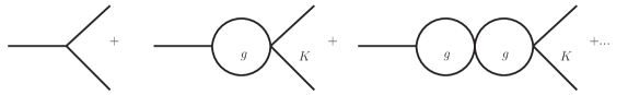
Figure 2: The s-channel diagrams to the scalar $\pi\pi$ form factors in CHPT. With the increase of the $\pi\pi$ invariant mass, higher-order contributions may become important. In the unitarized approach Oller:1998hw , these diagrams can be summed.

With the increase of the invariant mass of the $\pi\pi$ system, higher order contributions become more important. It has been proposed that the unitarized approach which can sum higher order corrections and extend the applicability to the scale around 1 GeV Oller:1998hw . A sketch of the resummation scheme is shown in Fig. 2. In this figure, the $K(s)$ is the $S$-wave projected kernel of meson-meson scattering amplitudes Gasser:1983yg ; Gasser:1984gg :

$$K(s)=\left(\begin{array}[]{cc}K_{11}&K_{12}\\ K_{21}&K_{22}\end{array}\right),$$ (30)

$$K_{11}=\frac{2s-m_{\pi}^{2}}{2f^{2}},\quad K_{12}=K_{21}=\frac{\sqrt{3}s}{4f^{2}},\;\;\;K_{22}=\frac{3s}{4f^{2}},$$ (31)

where the subscript $1,2$ denotes the $\pi\pi$ and $K\bar{K}$ state respectively. The function $g(s)$ is the loop integral which can be calculated in the cutoff-regularization scheme with $q_{\rm max}\sim 1$GeV being the cutoff [cf. Erratum of Ref. Oller:1998hw ] or in dimensional regularization. In the latter scheme, the meson loop function $g_{ii}(s)$ is given by

$$J_{ii}^{r}(s)\! \equiv \!\frac{1}{16\pi^{2}}\left[1-\log\left(\frac{m_{i}^{2}}{\mu^{2}}\right)-\sigma_{i}(s)\log\left(\frac{\sigma_{i}(s)+1}{\sigma_{i}(s)-1}\right)\right]=-g_{ii}(s).$$ (32)

with $\sigma_{i}(s)=\sqrt{1-{4m_{i}^{2}}/{s}}$. Imposing the unitarity constraints, the scalar form factor can be expressed in terms of the algebraic coupled-channel equation Meissner:2000bc ; Lahde:2006wr

$$F(s) = R(s)[I+g(s)K(s)]^{-1}$$ (33)

$$= R(s)[I-g(s)K(s)]\>+\>\mathcal{O}(p^{6}),$$

where the above equation has been expanded up to NLO in the chiral expansion. The $R(s)=(R_{1}(s),R_{2}(s))$ includes both tree-level contributions, and other higher order corrections that have not been summed. Thus this function has no right-hand cut, and can be obtained by matching onto the CHPT results in Eqs. (27,27) Oller:1997ti ; Lahde:2006wr :

$$R_{1}(s)\>\>= \frac{\sqrt{3}}{\>2}\left\{\frac{16m_{\pi}^{2}}{f^{2}}\left(2L_{6}^{r}-L_{4}^{r}\right)+\frac{8s}{f^{2}}L_{4}^{r}-\frac{m_{\pi}^{2}}{72\pi^{2}f^{2}}\left[1+\log\left(\frac{m_{\eta}^{2}}{\mu^{2}}\right)\right]\right\},$$ (35)

$$R_{2}(s)\>\>= 1+\frac{8L_{4}^{r}}{f^{2}}\left(s-4m_{K}^{2}-m_{\pi}^{2}\right)+\frac{4L_{5}^{r}}{f^{2}}\left(s-4m_{K}^{2}\right)+\frac{16L_{6}^{r}}{f^{2}}\left(4m_{K}^{2}+m_{\pi}^{2}\right)+\frac{32L_{8}^{r}}{f^{2}}m_{K}^{2}+\frac{2}{3}\mu_{\eta}$$

$$+\frac{m_{K}^{2}}{36\pi^{2}f^{2}}\left[1+\log\left(\frac{m_{\eta}^{2}}{\mu^{2}}\right)\right].$$

With the above formulae and the fitted results for the low-energy constants $L_{i}^{r}$ in Ref. Lahde:2006wr (evolved from $m_{\rho}$ to the scale $\mu=2q_{\rm max}/\sqrt{e}$), we show the strange $\pi\pi$ form factor in Fig. 3. The modulus, real part and imaginary part are shown as solid, dashed and dotted curves.

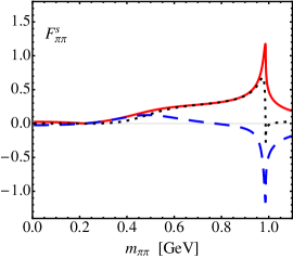
Figure 3: The $\pi\pi$ scalar form factor obtained in the unitarized chiral perturbation theory. The modulus, real part and imaginary part are shown in solid, dashed and dotted curves.

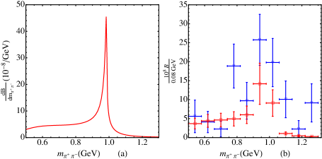
Figure 4: The differential branching ratio for the $B_{s}\to\pi^{+}\pi^{-}\ell^{+}\ell^{-}$. The experimental data (with triangle markers) has been normalized to the central value of the branching fraction: ${\cal B}(B_{s}^{0}\to\pi^{+}\pi^{-}\mu^{+}\mu^{-})=(8.6\pm 1.5\pm 0.7\pm 0.7)\times 10^{-8}$. Theoretical predictions (with square markers) are based on the result for the time-like scalar form factors derived in the unitarized CHPT.

Equipped with the results for scalar form factor and heavy to light transition, we can explore the differential branching fraction for the $B_{s}\to\pi^{+}\pi^{-}\mu^{+}\mu^{-}$. Our theoretical results for $d{\cal B}/dm_{\pi\pi}$ is given in the left panel of Fig. 4. This clearly shows the peak corresponding to the $f_{0}(980)$. In order to compare with the experimental data, we also give the binned results on the right panel in Fig. 4 from $0.5$ GeV to $1.3$ GeV. Theoretical errors shown in this panel arise from the ones in the form factors. The experimental data (with triangle markers) has been normalized to the central value given in Eq. (1). The comparison in this panel shows a general agreement between our theoretical prediction and the experimental data except in a few bins. This agreement is very encouraging.

In spite of the agreement, there exist some differences in our results and data. For instance our theoretical result does not show the enhancement at $m_{\pi\pi}\simeq(800,1100,1250)$MeV as given in the data. The excess at $800$ MeV may come from the tail of the $B_{s}\to\eta(\to\pi^{+}\pi^{-}\pi^{0},\pi^{+}\pi^{-}\gamma)\mu^{+}\mu^{-}$, while in the range above 1GeV, the contribution from the $f_{0}(1370)$ may not be negligible.

Integrating out the $m_{\pi\pi}$, we have the branching fraction:

$${\cal B}(B_{s}\to f_{0}(980)(\to\pi^{+}\pi^{-})\mu^{+}\mu^{-})=(4.1\pm 1.6)\times 10^{-8},$$ (36)

which deviates from the data by about $2\sigma$. However, one expects the experimental result in Eq. (2) would get somewhat reduced. This can be witnessed by the $B^{-}\to J/\psi K^{-}$ and $B^{-}\to K^{-}\mu^{+}\mu^{-}$ Agashe:2014kda

$$\frac{{\cal B}(B^{-}\to K^{-}\mu^{+}\mu^{-})}{{\cal B}(B^{-}\to J/\psi K^{-})}=\frac{(4.49\pm 0.23)\times 10^{-7}}{(1.027\pm 0.031)\times 10^{-3}}\sim 4.4\times 10^{-4}.$$ (37)

If this ratio were not sensitive the light meson in the final state which is true in most cases, the branching fraction for the $B_{s}\to J/\psi f_{0}(980)$ Agashe:2014kda

$${\cal B}(B_{s}\to J/\psi f_{0})=(1.39\pm 0.14)\times 10^{-4},$$

would indicate

$${\cal B}(B_{s}\to f_{0}(980)\mu^{+}\mu^{-})\sim 6.1\times 10^{-8}.$$ (38)

This value is smaller by about $30\%$ than the central value given in Eq. (1), and is more consistent with our theoretical result. The future measurement with more data at the experimental facilities like LHC and KEKB will be able to clarify this point, and thus to examine our theoretical formalism more precisely. We strongly encourage our experimental colleagues to conduct such measurements.

In summary, in this work we have analyzed the $B_{s}\to\pi^{+}\pi^{-}\ell^{+}\ell^{-}$ that has focused on the region where the pion pairs have invariant mass in the range $0.5$-$1.3$ GeV and muon pairs do not originate from a resonance. We have adopted the approach proposed in our previous work Meissner:2013hya ; Meissner:2013pba ; Doring:2013wka (see also Ref. Wang:2014sba for an overview) which makes uses of the two-hadron light-cone distribution amplitude. The scalar $\pi^{+}\pi^{-}$ form factor induced by the strange $\bar{s}s$ current is predicted by the unitarized chiral perturbation theory. The heavy to light transition can then be handled by the light-cone sum rules approach. Merging these quantities, we have presented our theoretical results for differential decay width and compared with the experimental data. Except in a few bins, our theoretical results are in alignment with the data. We have also discussed the disagreement and given our expectation. More accurate measurements at the LHC and KEKB in future are helpful to validate/falsify our formalism and determine the inputs in this approach.

Acknowledgements: The authors thank Michael Döring, Feng-Kun Guo, Bastian Kubis, Hsiang-Nan Li, Cai-Dian Lü, Ulf-G. Meissner, Eulogio Oset, Wen-Fei Wang for enlightening discussions. This work was supported in part by a key laboratory grant from the Office of Science and Technology, Shanghai Municipal Government (No. 11DZ2260700), and by Shanghai Natural Science Foundation under Grant No.15ZR1423100.

References

• (1) R. Aaij et al. [LHCb Collaboration], arXiv:1412.6433 [hep-ex].
• (2) U. G. Meißner and W. Wang, Phys. Lett. B 730, 336 (2014) [arXiv:1312.3087 [hep-ph]].
• (3) U. G. Meißner and W. Wang, JHEP 1401, 107 (2014) [arXiv:1311.5420 [hep-ph]].
• (4) M. Döring, U. G. Meißner and W. Wang, JHEP 1310, 011 (2013) [arXiv:1307.0947 [hep-ph]].
• (5) W. Wang, Int. J. Mod. Phys. A 29, 1430040 (2014) [arXiv:1407.6868 [hep-ph]].
• (6) S. Gardner and U. G. Meißner, Phys. Rev. D 65, 094004 (2002) [hep-ph/0112281].
• (7) M. Maul, Eur. Phys. J. C 21, 115 (2001) [hep-ph/0104078].
• (8) C. H. Chen and H. n. Li, Phys. Lett. B 561, 258 (2003) [hep-ph/0209043].
• (9) C. H. Chen and H. n. Li, Phys. Rev. D 70, 054006 (2004) [hep-ph/0404097].
• (10) W. F. Wang, H. C. Hu, H. n. Li and C. D. Lü, Phys. Rev. D 89, 074031 (2014) [arXiv:1402.5280 [hep-ph]].
• (11) H. s. Wang, S. m. Liu, J. Cao, X. Liu and Z. j. Xiao, Nucl. Phys. A (2014).
• (12) W. F. Wang, H. n. Li, W. Wang and C. D. L , arXiv:1502.05483 [hep-ph].
• (13) K. A. Olive et al. [Particle Data Group Collaboration], Chin. Phys. C 38, 090001 (2014).
• (14) C. D. Lu and W. Wang, Phys. Rev. D 85, 034014 (2012) [arXiv:1111.1513 [hep-ph]].
• (15) P. Colangelo, F. De Fazio and W. Wang, Phys. Rev. D 81, 074001 (2010) [arXiv:1002.2880 [hep-ph]].
• (16) D. Müller, D. Robaschik, B. Geyer, F.-M. Dittes and J. Ho?ej i, Fortsch. Phys.  42, 101 (1994) [hep-ph/9812448].
• (17) M. Diehl, T. Gousset, B. Pire and O. Teryaev, Phys. Rev. Lett.  81, 1782 (1998) [hep-ph/9805380].
• (18) M. V. Polyakov, Nucl. Phys. B 555, 231 (1999) [hep-ph/9809483].
• (19) N. Kivel, L. Mankiewicz and M. V. Polyakov, Phys. Lett. B 467, 263 (1999) [hep-ph/9908334].
• (20) M. Diehl, Phys. Rept.  388, 41 (2003) [hep-ph/0307382].
• (21) P. Hagler, B. Pire, L. Szymanowski and O. V. Teryaev, Phys. Lett. B 535, 117 (2002) [Erratum-ibid. B 540, 324 (2002)] [hep-ph/0202231].
• (22) B. Pire, F. Schwennsen, L. Szymanowski and S. Wallon, Phys. Rev. D 78, 094009 (2008) [arXiv:0810.3817 [hep-ph]].
• (23) P. Colangelo and A. Khodjamirian, In *Shifman, M. (ed.): At the frontier of particle physics, vol. 3* 1495-1576 [hep-ph/0010175].
• (24) H. Y. Cheng, C. K. Chua and K. C. Yang, Phys. Rev. D 73, 014017 (2006) [hep-ph/0508104].
• (25) Y. J. Sun, Z. H. Li and T. Huang, Phys. Rev. D 83, 025024 (2011) [arXiv:1011.3901 [hep-ph]].
• (26) H. Y. Han, X. G. Wu, H. B. Fu, Q. L. Zhang and T. Zhong, Eur. Phys. J. A 49, 78 (2013) [arXiv:1301.3978 [hep-ph]].
• (27) Z. G. Wang, arXiv:1409.6449 [hep-ph].
• (28) Y. Y. Keum, H. n. Li and A. I. Sanda, Phys. Lett. B 504, 6 (2001) [hep-ph/0004004].
• (29) Y. Y. Keum, H. N. Li and A. I. Sanda, Phys. Rev. D 63, 054008 (2001) [hep-ph/0004173].
• (30) T. Kurimoto, H. n. Li and A. I. Sanda, Phys. Rev. D 65, 014007 (2002) [hep-ph/0105003].
• (31) C. D. Lu, K. Ukai and M. Z. Yang, Phys. Rev. D 63, 074009 (2001) [hep-ph/0004213].
• (32) C. D. Lu and M. Z. Yang, Eur. Phys. J. C 23, 275 (2002) [hep-ph/0011238].
• (33) C. D. Lu and M. Z. Yang, Eur. Phys. J. C 28, 515 (2003) [hep-ph/0212373].
• (34) R. H. Li, C. D. Lu, W. Wang and X. X. Wang, Phys. Rev. D 79, 014013 (2009) [arXiv:0811.2648 [hep-ph]].
• (35) F. De Fazio and M. R. Pennington, Phys. Lett. B 521, 15 (2001) [hep-ph/0104289].
• (36) H. Y. Cheng, C. K. Chua, K. C. Yang and Z. Q. Zhang, Phys. Rev. D 87, no. 11, 114001 (2013) [arXiv:1303.4403 [hep-ph]].
• (37) J. Gasser and U. G. Meißner, Nucl. Phys. B 357, 90 (1991).
• (38) U. G. Meißner and J. A. Oller, Nucl. Phys. A 679, 671 (2001) [hep-ph/0005253].
• (39) J. Bijnens and P. Talavera, Nucl. Phys. B 669, 341 (2003) [hep-ph/0303103].
• (40) T. A. Lahde and U. G. Meißner, Phys. Rev. D 74, 034021 (2006) [hep-ph/0606133].
• (41) Z. H. Guo, J. A. Oller and J. Ruiz de Elvira, Phys. Rev. D 86, 054006 (2012) [arXiv:1206.4163 [hep-ph]].
• (42) J. Gasser and H. Leutwyler, Annals Phys.  158, 142 (1984).
• (43) J. Gasser and H. Leutwyler, Nucl. Phys. B 250, 465 (1985).
• (44) J. Gasser and H. Leutwyler, Nucl. Phys. B 250, 517 (1985).
• (45) J. F. Donoghue, J. Gasser and H. Leutwyler, Nucl. Phys. B 343, 341 (1990).
• (46) J. A. Oller, E. Oset and J. R. Pelaez, Phys. Rev. D 59, 074001 (1999) [Erratum-ibid. D 60, 099906 (1999)] [Erratum-ibid. D 75, 099903 (2007)] [hep-ph/9804209].
• (47) J. A. Oller and E. Oset, Nucl. Phys. A 620, 438 (1997) [Erratum-ibid. A 652, 407 (1999)] [hep-ph/9702314].