Chandra and XMM-Newton Observations of the Bimodal Planck SZ-detected Cluster PLCKG345.40-39.34 (A3716) with High and Low Entropy Subcluster Cores

Abstract

We present results from Chandra, XMM-Newton, and ROSAT observations of the Planck SZ-detected cluster A3716 (PLCKG345.40-39.34 – G345). We show that G345 is, in fact, two subclusters separated on the sky by 400 kpc. We measure the subclusters’ gas temperatures ($\sim$ 2–3 keV), total ($\sim$ 1–2 $\times 10^{14}~{}M_{\odot}$) and gas ($\sim$ 1–2 $\times 10^{13}~{}M_{\odot}$) masses, gas mass fraction within $r_{500}$, entropy profiles, and X-ray luminosities ($\sim 10^{43}\rm~{}erg~{}s^{-1}$). Using the gas density and temperature profiles for both subclusters, we show that there is good ($0.8\sigma$) agreement between the expected Sunyaev-Zel’dovich signal predicted from the X-ray data and that measured from the Planck mission, and better agreement within $0.6\sigma$ when we re-computed the Planck value assuming a two component cluster model, with relative amplitudes fixed based on the X-ray data. Dynamical analysis shows that the two galaxy subclusters are very likely ($>97\%$ probability) gravitationally bound, and in the most likely scenario, the subclusters will undergo core passage in $500\pm 200$ Myr. The northern subcluster is centrally peaked and has a low entropy core, while the southern subcluster has a high central entropy. The high central entropy in the southern subcluster can be explained either by the mergers of several groups, as suggested by the presence of five giant ellipticals or by AGN energy injection, as suggested by the presence of a strong radio source in one of its massive elliptical galaxies, or by a combination of both processes.

1. Introduction

Clusters of galaxies are the largest gravitationally bound structures in the Universe to have reached virial equilibrium. In the standard $\Lambda$CDM cosmology, massive halos dominated by dark matter assemble by accretion of smaller groups and clusters. Under the influence of gravity, uncollapsed matter and smaller collapsed halos fall into larger halos and, occasionally, halos of comparable mass merge with one another. Observations of substructures in clusters of galaxies (e.g., Jones & Forman, 1984, 1999; Mohr et al., 1995; Buote & Tsai, 1996; Jeltema et al., 2005; Laganá et al., 2010; Andrade-Santos et al., 2012, 2013) and the growth of structure (Vikhlinin et al., 2009) strongly suggest that clusters formed recently (Forman & Jones, 1982; Richstone et al., 1992). To better understand the evolution of the Universe, it is important to identify and characterize these large structures.

The first catalog of 189 Sunyaev-Zel’dovich (SZ) clusters detected by the Planck mission was released in early 2011 (Planck Collaboration et al., 2011). Through a Chandra XVP (X-ray Visionary Program – PI: Christine Jones) and HRC Guaranteed Time Observations (PI: Stephen S. Murray), which comprise the Chandra-Planck Legacy Program for Massive Clusters of Galaxies, we are obtaining Chandra exposures sufficient to collect at least 10,000 source counts for each of the ESZ Planck clusters at $z\leq 0.35$. PLCKG345.40-39.34 (hereafter G345 - RA = 20:52:16.8, DEC = -52:49:30.7) is a nearby cluster (z = 0.045). G345 was the first cluster observed as part of the Chandra XVP, which revealed it to be a double cluster (we distinguish the north and south subclusters as G345N and G345S, respectively).

Historically, Abell et al. (1989) had catalogued a single cluster of galaxies (A3716 – cross mark in Figure 1) located $\sim 6^{\prime}$ northwest of G345S and $\sim 6^{\prime}$ southwest of G345N.

Figure 1.— Left: 0.5–2.0 keV XMM-Newton image of G345. Right: ESO DSS-Red optical image of the same sky region presented in the left panel. Isointensity X-ray contours are shown in both panels. The cross indicates the Abell et al. (1989) catalogue position for A3716.

In Section 2 of this paper we present the Chandra, XMM-Newton, and ROSAT observations and data reduction. In Section 3 we describe the X-ray spatial and spectral analysis. The total mass and gas mass for each subcluster are presented in Section 4, and the entropy profiles of both subclusters are computed in Section 5. In Section 6 we compute the expected Sunyaev-Zel’dovich signal from the X-ray data, as well as a comparison between the X-ray emission and the Planck reconstructed Sunyaev-Zel’dovich map. Finally, we present a dynamical model for the two subclusters in Section 7 and the conclusions in Section 8.

We assume a standard $\Lambda$CDM cosmology with $\Omega_{\rm M}=0.3$, $\Omega_{\Lambda}=0.7$ and $H_{0}=70$ km s^-1Mpc^-1, implying a linear scale of $0.89\rm\ kpc\ arcsec^{-1}$ at the G345 luminosity distance of 199 Mpc ($z=0.045$).

Table 1Best Fit Parameters for the $\beta$-Model and central density.

Subcluster	$r_{\rm c}$	$\beta$	$n_{\rm e,0}$	$\rho_{0}$
	(kpc)		($\rm cm^{-3}$)	($\rm g~{}cm^{-3}$)
G345N	118 $\pm$ 9	0.54 $\pm$ 0.02	$(3.19\pm 0.28)\times 10^{-3}$	$(6.21\pm 0.54)\times 10^{-27}$
G345S	228 $\pm$ 12	0.48 $\pm$ 0.01	$(8.96\pm 0.51)\times 10^{-4}$	$(1.74\pm 0.10)\times 10^{-27}$

Note. — Columns list subclusters’ names, determination and 1$\sigma$ uncertainties for the core radius, $\beta$ (Equation (1)), and central electron number and gas mass densities (Equation (4)).

Table 2Comparison Between the Best Fit Parameters for the $\beta$-Model Using Different Data Sets.

Telescope	Subcluster	$r_{\rm c}$	$\beta$	$\chi^{2}_{\rm red}$
		(kpc)
Chandra	G345N	$82\pm 23$	$0.44\pm 0.08$	0.83
	G345S	$228\pm 49$	$0.44\pm 0.04$	1.37
XMM-Newton	G345N	$91\pm 33$	$0.46\pm 0.10$	1.05
	G345S	$199\pm 20$	$0.45\pm 0.02$	1.73
Chandra + XMM-Newton + ROSAT	G345N	118 $\pm$ 9	0.54 $\pm$ 0.02	1.07
	G345S	228 $\pm$ 12	0.48 $\pm$ 0.01	1.31

Note. — Columns list telescope data used for fitting the surface brightness profile, subclusters names, best fit for the core radius, $\beta$ (Equation (1)), and reduced $\chi$-square.

2. X-ray Observations and data reduction

2.1. Chandra

We observed G345 on November 21 and 26, 2012, with the Chandra X-ray Observatory (ACIS-I detectors, VF mode, ObsIds 15133 (catalog ADS/Sa.CXO#obs/15133) – 15 ks – and 15583 (catalog ADS/Sa.CXO#obs/15583) – 15 ks – see center panel of Figure 2). The data were reduced following the processing described in Vikhlinin et al. (2005), applying the calibration files CALDB 4.5.3. The data processing includes corrections for the time dependence of the charge transfer inefficiency and gain, and a check for periods of high background (none were found). Also, readout artifacts were subtracted and standard blank sky background files were used for background subtraction.

2.2. XMM-Newton

We observed G345 on April 2, 2013, with the XMM-Newton  Observatory for 22.7 ks (ObsId 0692930101). We used the images script from the XMM-Newton website to create exposure corrected images of the cluster in the 0.5–2.0 keV energy band. This script removes periods of high background, as well as bad pixels and columns, spatially smooths and exposure corrects the data and merges PN and MOS observations (see Figure 1 left panel and Figure 2 right panel).

2.3. ROSAT

G345 was observed on April 2, 1991 for 2.7 ks (ObsId RP800042A00) and on April 1, 1992 for 1.6 ks (ObsId RP800042A01) with the ROSAT PSPC. We used available hard band (0.4–2.4 keV) images, background, and exposure maps to create a background subtracted, exposure corrected image of the cluster that we used to constrain the subclusters’ surface brightness profiles at large radii (see Figure 2 left panel).

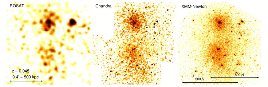
Figure 2.— Left: The 0.4–2.4 keV ROSAT PSPC image of G345. Center: The 0.5–2.0 keV Chandra image of G345. Right: The 0.5–2.0 keV XMM-Newton image of G345 showing $r_{500}$ for each subcluster. All three images have the same spatial scale.

3. Spatial and Spectral Analysis

3.1. X-ray Surface Brightness Radial Profiles

The surface brightness is the projection of the plasma emissivity along the line of sight. We fit the X-ray surface brightness radial profile of each G345 subcluster with a $\beta$-model (Cavaliere & Fusco-Femiano, 1976) which is well suited for non-cool-core relaxed clusters. This model is defined as:

$$S(r)=S_{0}\left[1+\left(\frac{r}{r_{c}}\right)^{2}\right]^{-3\beta+0.5},$$ (1)

where $r_{c}$ is the core radius, $\beta$ is the shape parameter, and $S_{0}$ is the central surface brightness. Figure 3 shows the surface brightness profiles for the northern (left panel) and southern (right panel) subclusters, along with the best $\beta$-model fits. We detect X-ray emission from Chandra and XMM-Newton to a radius of $\sim$ 700 kpc for the northern component and to $\sim$ 1 Mpc for the southern one. The background level is $(1.70\pm 0.13)\times 10^{-7}\rm~{}counts~{}s^{-1}~{}arcsec^{-2}$ (normalized to the Chandra ACIS-I count rate sensitivity in the 0.5–2.0 keV energy band). For G345N, we modeled the X-ray surface brightness with the addition of a Gaussian function to describe the X-ray emission associated with the central giant elliptical (ESO 187-G026). The Gaussian function in the Chandra fit describes the bright core, whereas in the case of XMM-Newton fit, the Gaussian function is broader due to the telescope’s larger PSF compared to Chandra. With Chandra, we extracted a spectrum from a circle of 7 kpc (7.9^′′) in radius centered on ESO 187-G026 to estimate the gas temperature of the bright central region (using the spectrum from an annulus with inner and outer radii of 7 (7.9^′′) and 27 kpc (30.5^′′) respectively, as the background component to properly subtract the cluster emission). For the galaxy, we obtain $kT=0.92^{+0.13}_{-0.15}$ keV and $L_{\rm X}=2.62^{+0.02}_{-1.16}\times 10^{41}\rm~{}erg~{}s^{-1}$. In the Appendix we show that the (stellar + LMXB) luminosity of this galaxy is $L_{\rm 0.5-2.0~{}keV}=1.74\times 10^{40}\rm~{}erg~{}s^{-1}$ which is only $\sim 7\%$ of the total 0.5–2.0 keV luminosity within 7 kpc (7.9^′′) of its center. Thus, the majority of the X-ray emission comes from diffuse gas. In a similar way, Vikhlinin et al. (2001) showed that there are $\sim$ 3 kpc cores of 1–2 keV gas in both giant ellipticals (NGC4874 and NGC4889) in the massive and hot ($kT\sim 8$ keV) Coma cluster, and Sun et al. (2007) presented a systematic investigation of X-ray thermal coronae in a survey of 25 nearby clusters. They showed that cool galactic coronae ($kT$ = 0.5–1.0 keV generally) are common in cluster cores. Using ROSAT’s larger field of view to better constrain the background level along with Chandra and XMM-Newton observations, we fitted each subcluster X-ray surface brightness to a $\beta$-model profile and determined $\beta$ and $r_{\rm c}$ (the background level for each surface brightness profile (Chandra, XMM-Newton, and ROSAT) was free to vary independently, while $r_{\rm c}$ and $\beta$ were tied to a single best fit value). For G345N, we obtained $\beta$ = 0.54 $\pm$ 0.02  and $r_{\rm c}$ = 118 $\pm$ 9  kpc ($\chi^{2}_{\rm red}=1.07$), and for G345S, we obtained $\beta$ = 0.48 $\pm$ 0.01  and $r_{\rm c}$ = 228 $\pm$ 12  kpc ($\chi^{2}_{\rm red}=1.31$). We also fit the Chandra and XMM-Newton profiles individually and found consistent $\beta$ and $r_{\rm c}$. The best fit parameters are summarized in Table 1. The southern subcluster has a flatter $\beta$ and a larger core radius than the northern subcluster, which along with the poorer $\beta$-model fit and higher central entropy of G345S (the entropy profiles for each subcluster will be discussed in Section 5) suggest this subcluster is still in the process of forming. However, visual inspection of Figure 3 as well as the best fit reduced $\chi^{2}$ show that the $\beta$-model describes well the X-ray surface brightness profiles of G345N (with the exception of the central region due to the central galaxy’s cool galactic corona X-ray emission) and G345S, validating the assumption that the gas density defined by the surface brightness follows this model.

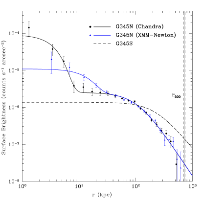
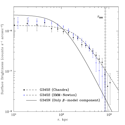
Figure 3.— Left: X-ray background-subtracted surface brightness profiles and fits for G345N (solid lines), along with the surface brightness fit for G345S (dashed line). The difference between the profiles in the core is due to the XMM-Newton poorer angular resolution compared to that of Chandra. The Gaussian function in the Chandra fit describes the cool galactic corona. For XMM-Newton the Gaussian function to describe the core is broader, corresponding to the telescope’s larger PSF. Right: X-ray surface brightness profile of G345S (dashed line), along with the surface brightness fit for the G345N cluster component (solid line) for comparison. For each profile, regions in the direction of the other subcluster are excluded. For display purpose, the XMM-Newton central surface brightness in the $\beta$-model was normalized to match the central surface brightness in the Chandra fit. The background level is $(1.70\pm 0.13)\times 10^{-7}\rm~{}counts~{}s^{-1}~{}arcsec^{-2}$ (normalized to the Chandra ACIS-I count rate sensitivity in the 0.5–2.0 keV energy band).

3.2. Gas Density Radial Profiles

The $\beta$-model gas density distribution that corresponds to the surface brightness distribution given by Equation (1) is:

$$\rho_{\rm g}(r)=\rho_{\rm g,0}\left[1+\left(\frac{r}{r_{\rm c}}\right)^{2}\right]^{-3\beta/2},$$ (2)

where $\rho_{\rm g,0}$ is the central gas density. The core radius, $r_{\rm c}$, and $\beta$ are constrained from fitting the X-ray surface brightness profile.

The gas mass within $r_{500}$ (the radius defining a sphere whose interior mean mass density is 500 times the critical density at the cluster redshift – see Section 4) is then given by:

$$M_{\rm g,500} =4\pi\rho_{g,0}\int_{0}^{r_{500}}\left[1+\left(\frac{r}{r_{\rm c}}\right)^{2}\right]^{-3\beta/2}r^{2}dr$$ (3)

$$=\frac{4\pi}{3}\rho_{g,0}r_{500}^{3}~{}_{2}F_{1}(3/2,3\beta/2;5/2;-y^{2}),$$

where $y=r_{500}/r_{\rm c}$ and ${}_{2}F_{1}(a,b;c;d)$ is the Gauss hypergeometric function. For a plasma with a given electron to hydrogen number densities ratio $n_{\rm e}/n_{\rm H}$, the central electron number density, $n_{\rm e,0}$ is calculated as:

$$n_{\rm e,0}=\left(\frac{K(n_{\rm e}/n_{\rm H})[D_{\rm A}(1+z)]^{2}(6\beta-3)\times 10^{14}}{2^{6\beta-3}r_{\rm c}^{3}B(3\beta-1/2,3\beta-1/2)}\right)^{1/2}\times$$

$$\left(\left[1+\left(\frac{R_{\rm i}}{r_{c}}\right)^{2}\right]^{-3\beta+3/2}-\left[1+\left(\frac{R_{\rm f}}{r_{c}}\right)^{2}\right]^{-3\beta+3/2}\right)^{-1/2}$$ (4)

where $D_{\rm A}$ is the angular distance of the cluster, $B(a,b)$ $a,b\in$ $\mathbb{R}$ is the Euler $\beta$ function, $R_{\rm i}$ and $R_{\rm f}$ are the projected initial and final radii of the annulus for which the spectrum has been fit and the normalization, $K$, was computed using the apec model in XSPEC. The relation between the gas density and electron number density is given by $\rho_{\rm g}=\mu_{\rm e}n_{\rm e}m_{\rm a}$, where $\mu_{\rm e}$ is the mean molecular weight per electron and $m_{\rm a}$ is the atomic mass unit. For a metallicity of 0.3 $Z_{\odot}$, using the reference values from Anders & Grevesse (1989) we obtain $\mu_{\rm e}=1.1706$ and $n_{\rm e}/n_{\rm H}=1.1995$. The central electron number and gas densities for G345N are approximately four times higher than those for G345S. These are given in Table 1.

3.3. Gas Temperature Radial Profiles

The temperature profiles of most clusters have a broad peak within 0.1–0.2 $r_{200}$ and decreases at larger radii, reaching approximately 50% of the peak value near $0.5\,r_{200}$ (Vikhlinin et al., 2006). In cool-core clusters there is also a temperature decline toward the cluster center due to radiative cooling. The analytic model constructed by Vikhlinin et al. (2006) for the 3D temperature profile describes these general features. However, due to the quality of our data, we employed a simplified form of this temperature profile with some of the parameters fixed (the universal temperature profile from Vikhlinin et al. (2006), but with the transition radius, $r_{t}$, allowed to vary). Thus

$$T_{\rm 3D}(r)=\frac{T_{0}}{[1+(r/r_{t})^{2}]}\times\frac{[r/(0.075r_{t})]^{1.9}+0.45}{[r/(0.075r_{t})]^{1.9}+1}.$$ (5)

Monte-Carlo simulations were performed to estimate the uncertainties in the best fit values for the parameters in this analytical model. This analytic model for $T_{\rm 3D}(r)$ (Equation (5)), allows very steep temperature gradients. In some realizations, such profiles are formally consistent with the observed projected temperatures because projection flattens steep gradients. However, steep values of $dT/dr$ often lead to unphysical mass estimates, for example, profiles with negative dark matter density at some radii. We addressed this problem in the Monte-Carlo simulations by accepting only those realizations in which the best-fit $T(r)$ leads to $\rho_{\rm tot}>\rho_{\rm gas}$ in the radial range $r\leq 1.5\,r_{500}$. Finally, in the same radial range, we verified that the temperature profiles corresponding to the mass uncertainty interval are all convectively stable, i.e., $d\ln T/d\ln\rho_{g}<2/3$.

Using XMM-Newton observations, we extracted spectra in three half annuli subtending 180 degrees on the side opposite to the companion subcluster, centered on each subcluster in the radial range from from 0 to $\sim$ 400–600 kpc for each subcluster. Each half annulus has at least 3000 source counts. We fit these with an absorbed apec model. The measured Galactic hydrogen column density in the direction of the cluster is $N_{\rm H}=2.51\times 10^{20}{\rm~{}cm^{-2}}$, which was kept fixed while fitting the spectra. We then followed the procedures described below to obtain the 2D and 3D temperature profiles. The measured 2D, fitted 2D, and 3D temperature profiles are presented in the left panel of Figure 4. The 2D temperature profile was computed by projecting the 3D temperature weighted by gas density using the spectroscopic-like temperature (a formula for the temperature which matches the spectroscopically measured temperature within a few percent, Mazzotta et al., 2004):

$$T_{\rm 2D}=T_{\rm spec}\equiv\frac{\int\rho_{\rm g}^{2}T_{\rm 3D}^{1/4}dz}{\int\rho_{\rm g}^{2}T_{\rm 3D}^{-3/4}dz}$$ (6)

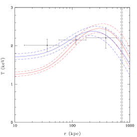
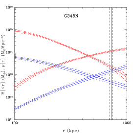
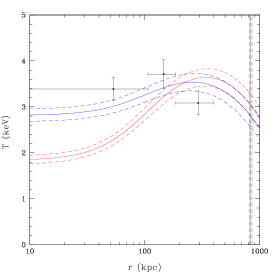
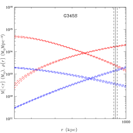
Figure 4.— Top: G345N. Bottom: G345S. Left: Temperature profiles. Measured projected temperatures are shown by circles with error bars. Solid red and blue lines show the best fit 3D model and the corresponding projected profile, respectively. Center: Mass and density profiles ($M(<r)$ increases with radius while $\rho(r)$ decreases). Red and blue lines show the results for the total mass and gas mass, respectively. Right: Gas mass fraction as a function of radius. Solid line shows the enclosed $f_{\rm gas}=M_{\rm g}(<r)/M_{\rm tot}(<r)$. The vertical line shows the radius $r_{500}$ derived from the best fit mass model assuming hydrostatic equilibrium. The dashed lines show the 68$\%$ confidence level limits for the best fits.

The spectroscopic-like temperature was also computed in the (0.15 – 1) $r_{500}$ range using the model for the 3D temperature and the gas density profile. For G345N, we found $kT=~{}$$2.11\pm 0.16$ keV, and for G345S, $kT=~{}$$2.85\pm 0.20$ keV.

Table 3Temperature Determination

Subcluster	$r$ (kpc)	$kT$ (keV)	Subcluster	$r$ (kpc)	$kT$ (keV)
	14.5 – 58.5	$2.01\pm 0.15$		0 – 106.8	$3.39\pm 0.25$
G345N	58.5 – 172.7	$2.15\pm 0.11$	G345S	106.8 – 186.0	$3.71\pm 0.31$
	172.7 – 591.5	$2.21\pm 0.27$		186.0 – 398.4	$3.08\pm 0.26$

Note. — Columns give subclusters’ names, radial range for the annuli used for temperature extraction, and the measured temperatures with 1$\sigma$ uncertainties.

Table 4Parameters for the Temperature Profile

Subcluster	$T_{0}$	$r_{\rm t}$
	(keV)	(kpc)
G345N	2.74 $\pm$ 0.14	1266 $\pm$ 243
G345S	4.07 $\pm$ 0.22	1459 $\pm$ 141

Note. — Columns list best fit values for $T_{0}$ and $r_{\rm t}$ given by Equation (5).

4. Total and Gas Masses of Subclusters

Given the three-dimensional models for the gas density and temperature profiles, the total mass within a radius $r$ can be computed for each subcluster from the equation for hydrostatic equilibrium (e.g., Sarazin 1988),

$$M(r) = \frac{-kTr}{\mu m_{H}G}\left(\frac{d\ln\rho_{\rm g}}{d\ln r}+\frac{d\ln T}{d\ln r}\right)$$ (7)

$$= -3.67\times 10^{13}~{}M_{\odot}kTr\left(\frac{d\ln\rho_{\rm g}}{d\ln r}+\frac{d\ln T}{d\ln r}\right),$$

where $k$ is the Boltzmann constant, $T$ is the gas temperature in units of K, and $r$ is in units of Mpc (the normalization corresponds to $\mu=0.6107$, appropriate for 0.3 $Z_{\odot}$).

Using Equation (7), $r_{500}$ is computed by solving

$$M(r_{500})=500\rho_{c}(4\pi/3)r_{500}^{3},$$ (8)

where $\rho_{c}$ is the critical density of the Universe at the cluster redshift. For G345N, we obtain $r_{500}=~{}$$724\pm 23$ kpc and a corresponding hydrostatic mass of $M_{\rm 500,hyd}=~{}$$(1.13\pm 0.11)\times 10^{14}$$M_{\odot}$. For G345S, we find $r_{500}=~{}$$836\pm 25$ kpc with a corresponding hydrostatic mass of $M_{\rm 500,hyd}=~{}$$(1.73\pm 0.15)\times 10^{14}$$M_{\odot}$. Using the best fit parameters for the $\beta$-model (see Table 1), we compute a gas mass within $r_{500}$ of $M_{\rm g,500}=~{}$$(1.45\pm 0.23)\times 10^{13}$$M_{\odot}$ for G345N, and $M_{\rm g,500}=~{}$$(1.45\pm 0.14)\times 10^{13}$$M_{\odot}$ for G345S.

The gas and total masses and density profiles, as well as the gas mass fractions within $r_{500}$ for both G345N and G345S are shown in the center and right panels of Figure 4. The gas mass fraction within $r_{500}$ is $f_{\rm g}=~{}$$0.084\pm 0.008$ for G345S and is in agreement with the expected value from Vikhlinin et al. (2006) for clusters $\sim$ 1–2 $\times 10^{14}M_{\odot}$ ($f_{\rm g}\sim 0.09$), whereas the gas mass fraction for G345N is slightly larger, $f_{\rm g}=$$0.130\pm 0.023$. We measure the X-ray luminosity within 245 kpc and extrapolate to $r_{500}$ for both subclusters, using the best fit $\beta$-model parameters. For G345N, we obtain a bolometric X-ray luminosity $L_{X,r_{500}}=(2.65\pm 0.37)\times 10^{43}\rm~{}erg~{}s^{-1}$, and for G345S, we obtain $L_{X,r_{500}}=(3.72\pm 0.51)\times 10^{43}\rm~{}erg~{}s^{-1}$. These results are summarized in Table 5.

Alternatively, if we use the gas mass and temperature, the total mass can be estimated from the $Y_{X}$–$M$ scaling relation of Vikhlinin et al. (2009),

$$M_{\rm 500,Y_{X}}=E(z)^{-2/5}A_{\rm YM}\left(\frac{Y_{\rm X}}{3\times 10^{14}M_{\odot}{\rm keV}}\right)^{B_{\rm YM}},$$

(9)

where $Y_{\rm X}=M_{\rm g,500}\times kT_{\rm X}$, $M_{\rm g,500}$ is given by Equation (3), and $T_{\rm X}$ is the spectroscopic-like temperature (see Equation (6)) in the (0.15–1) $\times~{}r_{500}$ range, computed based on the model for the gas density and 3D temperature profiles. $A_{\rm YM}=5.77\times 10^{14}h^{1/2}M_{\odot}$ and $B_{\rm YM}=0.57$ (Maughan et al., 2012). Here, $M_{\rm Y_{X},500}$ is the total mass within $r_{500}$, and $E(z)=[\Omega_{\rm M}(1+z)^{3}+(1-\Omega_{\rm M}-\Omega_{\Lambda})(1+z)^{2}+\Omega_{\Lambda}]^{1/2}$ is the function describing the redshift evolution of the Hubble parameter. As for the mass determination assuming hydrostatic equilibrium, we estimated 1$\sigma$ uncertainties in the $Y_{\rm X}$ derived quantities using Monte Carlo simulations. We also added to the Monte Carlo procedure a 1$\sigma$ systematic uncertainty of 9% in the mass determination, as discussed by Vikhlinin et al. (2009).

Using Equations (8) and (9), we compute $r_{\rm 500,Y_{x}}$ = $771\pm 47$ kpc for G345N with a corresponding total mass of $M_{\rm 500,Y_{x}}=$$(1.37\pm 0.25)\times 10^{14}$$M_{\odot}$ and gas mass $M_{\rm g,500,Y_{X}}=~{}$$(1.62\pm 0.38)\times 10^{13}$$M_{\odot}$. For G345S, we obtain $r_{\rm 500,Y_{x}}$ = $793\pm 42$  kpc with a corresponding total mass of $M_{\rm 500,Y_{x}}=~{}$$(1.48\pm 0.24)\times 10^{14}$$M_{\odot}$, and gas mass $M_{\rm g,500,Y_{X}}=~{}$$(1.33\pm 0.21)\times 10^{13}$$M_{\odot}$, in agreement with results obtained assuming the cluster to be in hydrostatic equilibrium.

Using the $Y_{\rm X}$ relation, the gas mass fractions within $r_{500}$ are $f_{\rm g}=~{}$$0.117\pm 0.015$ for G345N and $f_{\rm g}=~{}$$0.090\pm 0.007$ for G345S. These values are consistent with gas fractions computed above assuming hydrostatic equilibrium. These results are summarized in Table 6.

Table 5Physical Properties Derived Assuming Hydrostatic Equilibrium

Subcluster	$r_{\rm 500,hyd}$	$M_{\rm g,500,hyd}$	$M_{\rm 500,hyd}$	$f_{\rm gas,hyd}$	$kT_{\rm spec}$	$L_{\rm X,245}$	$L_{\rm X,r_{500}}$
	(kpc)	($M_{\odot}$)	($M_{\odot}$)		(keV)	($10^{43}\rm~{}erg~{}s^{-1}$)	($10^{43}\rm~{}erg~{}s^{-1}$)
G345N	$724\pm 23$	$(1.45\pm 0.23)\times 10^{13}$	$(1.13\pm 0.11)\times 10^{14}$	$0.130\pm 0.023$	$2.11\pm 0.16$	$1.35\pm 0.08$	$2.65\pm 0.37$
G345S	$836\pm 25$	$(1.45\pm 0.14)\times 10^{13}$	$(1.73\pm 0.15)\times 10^{14}$	$0.084\pm 0.008$	$2.85\pm 0.20$	$1.01\pm 0.06$	$3.72\pm 0.51$

Note. — Columns list the cluster $r_{500}$, gas mass, total mass derived from the hydrostatic equilibrium equation (Equation (7)), gas fraction, spectroscopic-like temperature within (0.15 – 1) $\times~{}r_{\rm 500}$, and bolometric X-ray luminosities within 245 kpc radii and extrapolated to within $r_{500}$.

Table 6Physical Properties Derived from the $Y_{\rm X}$–$M$ scaling relation

Subcluster	$r_{\rm 500,Y_{X}}$	$M_{\rm g,500,Y_{X}}$	$M_{\rm 500,Y_{X}}$	$f_{\rm gas,Y_{X}}$	$kT_{\rm spec}$	$L_{\rm X,245}$	$L_{\rm X,r_{500}}$
	(kpc)	($M_{\odot}$)	($M_{\odot}$)		(keV)	($10^{43}\rm~{}erg~{}s^{-1}$)	($10^{43}\rm~{}erg~{}s^{-1}$)
G345N	$771\pm 47$	$(1.62\pm 0.38)\times 10^{13}$	$(1.37\pm 0.25)\times 10^{14}$	$0.117\pm 0.015$	$2.08\pm 0.17$	$1.35\pm 0.08$	$2.72\pm 0.44$
G345S	$793\pm 42$	$(1.33\pm 0.21)\times 10^{13}$	$(1.48\pm 0.24)\times 10^{14}$	$0.090\pm 0.007$	$2.90\pm 0.21$	$1.01\pm 0.06$	$3.58\pm 0.48$

Note. — Columns list the cluster $r_{500}$, gas mass, total mass derived from the $Y_{X}$ parameter (Equation (9)), gas fraction, spectroscopic-like temperature within (0.15 – 1) $\times~{}r_{\rm 500}$, and bolometric X-ray luminosities within 245 kpc radii and extrapolated to within $r_{500}$.

5. Subcluster Entropy Profiles

The entropy index of the intracluster gas is defined as

$$K=\frac{kT}{n_{\rm e}^{2/3}},$$ (10)

where $k$ is the Boltzmann constant, $T$ is the gas temperature, and $n_{\rm e}$ is the electron density. The entropy profile reflects the thermodynamic history of the cluster. The entropy increases when heat energy is deposited into the ICM, and decreases when radiative cooling carries heat energy away (Voit et al., 2005).

To better understand the thermodynamic history of the G345 subclusters, we computed their entropy profiles, which are presented in Figure 5. They are remarkably different. G345S has extremely high entropy in its core ($\sim 200\rm~{}keV~{}cm^{2}$) due to the extremely low gas density for its observed $\sim$ 3 keV temperature (typically, the central entropy of a relaxed cluster with $\sim 3$ keV gas temperature would be $\sim$ 10–30 $\rm~{}keV~{}cm^{2}$, Voit et al., 2005; McDonald et al., 2013).

Figure 5.— Left: Entropy profiles for G345N and G345S. They are remarkably different. G345S presents a very high central entropy profile. The corona of the central galaxy has been removed from the profile for G345N. Right: Dimensionless entropy profiles for G345N and G345S. We see that the entropy index of G345N is very close to the scaling relation $K/K_{500}=1.42(r/r_{500})^{1.1}$ at $r_{500}$. On the other hand, G345S exceeds this value at $r_{500}$, suggesting that non-gravitational processes are playing a significant role in the thermodynamics of the ICM even at large distances from the center of the cluster.

Here, we present two heating mechanisms that could explain an entropy increase in the ICM. In the first, clusters that have experienced recent major mergers can have high central entropies due to energy deposited in the ICM through shocks during the merger. The shock heating will produce an entropy increase, in the case of a merger of clusters of similar masses, that can be directly related to the Mach number by:

$$\ln\left(\frac{K_{\rm f}}{K_{\rm i}}\right) = \ln\left[1+\frac{2\gamma(M^{2}-1)}{\gamma+1}\right]$$ (11)

$$- \gamma\ln\left[\frac{(\gamma+1)M^{2}}{(\gamma+1)+(\gamma-1)(M^{2}-1)}\right],$$

where $K_{\rm i}$ and $K_{\rm f}$ are the initial and final entropies, respectively (Zel’dovich & Raizer, 1967).

Assuming that the central entropy index of G345S was similar to that of G345N before it was perturbed, one can put a well-defined requirement on the shock strength in the core to boost the central entropy by a factor of 3.47 (ratio of central entropies between the southern and northern subclusters). Inserting this entropy ratio into Equation (11), one obtains a high Mach number of $M=4.8$, which corresponds to $\sim 4300\rm~{}km~{}s^{-1}$ for a 3 keV cluster. This result is implausibly high (assuming that the mass density profile of G345S is described by a NFW profile with concentration parameter of 4, a point mass falling from infinity would arrive in the center of G345S with a velocity of $\sim 2600\rm~{}km~{}s^{-1}$). However, shocks are not the only way to raise the entropy in a merger. Dissipation of turbulence also can play an important role. In the case in which the gas entropy enhancement of the southern subcluster had been caused by a first violent encounter with the northern subcluster, the cool core ($kT\sim 0.9$ keV – as presented in Section 3.1) in the central galaxy of G345N (ESO 187-G026) could be the gas that survived core passage after a collision with the southern subcluster. However, such a high velocity encounter would have highly disturbed the X-ray morphologies of both G345 subclusters, which is not observed.

For comparison, we searched for other clusters that present a similar high central gas entropy ($K_{0}\geq 150\rm~{}keV~{}cm^{2}$) and low temperature ($kT\leq 3.2$ keV) in the work of Cavagnolo et al. (2009), and found: A160, A193, A400, A562, A2125, and ZWCL 1215. Each cluster shows evidence of recent merger activity. A160 ($z=0.0447$) has two giant ellipticals in the core, that probably are in the process of merging. A193 ($z=0.0485$) has a central galaxy with a triple nucleus (IC 1695, Seigar et al., 2003). Since the typical time scale for multiple nuclei to merge into a single one is on the order of a Gyr (Seigar et al., 2003), observing a triple nucleus is a strong indication of recent merger activity. A400 ($z=0.024$) is a well studied system which presents indications of merger activity (Beers et al., 1992). A562 ($z=0.11$) has a Wide Angle Tail (WAT – radio lobes which are bent due to ram pressure as the host galaxy moves through the intracluster gas, Douglass et al., 2011). This is also a strong indicator of merger activity. Chandra observations, together with multiwavelength data, indicate that the A2125 complex ($z=0.2465$) is probably undergoing major mergers (Wang et al., 2004). Finally, inspecting the VLA FIRST image of ZWCL 1215 ($z=0.075$), we notice a disturbed radio morphology associated with a galaxy (4C+04.41) that is probably merging from the southwest. However this is not strong evidence of a major merger.

Five of the six clusters with high central gas entropy and low temperature show strong indications of recent or ongoing merger activity which is likely responsible for the enhancement of the central gas entropy through shocks. This may suggest that the high central gas entropy of G345S also was caused by a recent merger. However, if this were a merger with the northern subcluster, we would expect to observe an increase in the central entropy of the northern subcluster, which is not observed, therefore making this scenario unlikely.

The core of G345S hosts five giant ellipticals (see Figure 1) (unlike G345N, which has a single dominant giant elliptical), suggesting that we are witnessing the formation of the southern subcluster as groups of galaxies are in the process of merging. This scenario can explain the high central entropy of G345S, as the merging of the groups heats the gas through shocks.

As an alternative to multiple mergers of groups, less violent and frequent energy deposition into the ICM could also produce a significant entropy enhancement. Isobaric heating is a reasonable approximation for a less violent energy deposition where the gas pressure remains roughly constant while part of the energy is converted into $pdV$ work, causing expansion of the gas, and part is transferred to internal energy, heating the gas. For isobaric heating, the added heat $\delta Q$ is related to the entropy increase by

$$\delta Q = \frac{5kT_{\rm f}m_{\rm heated}}{2\mu m_{\rm H}}\left[1-\left(\frac{K_{\rm i}}{K_{\rm f}}\right)^{3/5}\right]=7.9\times 10^{61}{\rm erg}\times$$ (12)

$$\left(\frac{kT_{\rm f}}{1{\rm keV}}\right)\left(\frac{0.6}{\mu}\right)\left(\frac{m_{\rm heated}}{10^{13}M_{\odot}}\right)\left[1-\left(\frac{K_{\rm i}}{K_{\rm f}}\right)^{3/5}\right],$$

where $m_{\rm heated}$ is the gas mass that has been heated (for isobaric heating, the heat increment equals the enthalpy increment and $T_{\rm i}/T_{\rm f}=(K_{\rm i}/K_{\rm f})^{3/5}$, giving the equation above).

A less violent and steady source of energy that could explain the high central entropy could be energy injection into the ICM from an internal source such as an AGN. We can estimate a global entropy by weighting the entropy by gas density:

$$<K>=\frac{\int K\rho_{\rm g}~{}dV}{\int\rho_{\rm g}~{}dV}.$$ (13)

Within $r_{500}\sim$ 800 kpc the ratio of $<K>$ between G345S and G345N is $\sim$ 1.8. From Equation (12), we compute that the added heat necessary to increase the entropy of G345S is $\sim 1.0\times 10^{62}\rm~{}erg$, which corresponds to an AGN power of $\sim 3.3\times 10^{45}$–$10^{46}\rm~{}erg~{}s^{-1}$ if all this energy has been injected into the ICM within 1 – 0.1 Gyr, respectively. The 843 MHz radio image from the SUMSS survey (Bock et al., 1999) of the G345 field shows a bright radio source associated with one of the elliptical galaxies (ESO 187-IG 025 NED05 in G345S). Its radio power is $P_{\rm 1.4~{}GHz}=1.4\times 10^{24}\rm~{}W~{}Hz^{-1}$, which corresponds to a cavity power of roughly $10^{43}$–$\times 10^{46}\rm~{}erg~{}s^{-1}$ (Bîrzan et al., 2008; O’Sullivan et al., 2011). Such an AGN would need to inject energy into the ICM for a couple of Gyrs to enhance the central gas entropy by a factor of 1.8, which also makes this scenario possible. Thus, either an AGN sustained over a few Gyrs or the merger of groups could increase the central entropy of G345S.

Departure from the scaling relation $K/K_{500}=1.42(r/r_{500})^{1.1}$ (Pratt et al., 2010) is indicative of non-gravitational processes, where $K_{500}$ is computed by:

$$K_{500} = 106~{}{\rm keVcm^{2}}\left(\frac{M_{500}}{10^{14}h_{70}^{-1}M_{\odot}}\right)^{2/3}\left(\frac{1}{f_{\rm b}}\right)^{2/3}$$

$$\times E(z)^{-2/3}h_{70}^{-4/3},$$

where $f_{\rm b}=0.15$ is the baryon fraction (this is the assumed value for the baryon fraction in the work of Pratt et al., 2010). The right panel of Figure 5 shows the dimensionless entropy profile of both G345 subclusters. We see that the entropy index of G345N is very close to the scaling relation $K/K_{500}=1.42(r/r_{500})^{1.1}$ around $r_{500}$. On the other hand, G345S largely exceeds this value at $r_{500}$, suggesting that non-gravitational processes are playing a significant role in the thermodynamics of the ICM even at $r_{500}$, supporting the scenario that multiple mergers of groups have boosted the entropy index of G345S through shocks.

6. Planck Determined and Expected Sunyaev-Zel’dovich Signals

In this section, we compare the measured and expected Sunyaev-Zel’dovich signals from G345.

The total Sunyaev-Zel’dovich signal is given by the integral of the Compton parameter, $Y=\int y~{}d\Omega$, where $\Omega$ is the solid angle, and the Compton parameter $y$ is given by:

$$y=\frac{\sigma_{\rm T}}{m_{\rm e}c^{2}}\int_{l}kT_{\rm e}(r)n_{\rm e}(r)~{}dl,$$ (15)

where $\sigma_{\rm T}$ is the Thomson cross section, $m_{\rm e}c^{2}$ is the electron rest mass energy, $l$ is the distance along the line of sight, and $k$ is the Boltzmann constant. The total Sunyaev-Zel’dovich signal also can be expressed as:

$$Y=\frac{\sigma_{\rm T}}{D_{\rm A}^{2}m_{\rm e}c^{2}}\int_{V}P~{}dV,$$ (16)

where $D_{\rm A}$ is the angular size distance of the cluster, and $P$ is the electron pressure, $P=n_{\rm e}kT_{\rm e}$. The spherical Sunyaev-Zel’dovich signal measured by the Planck mission is $Y=0.0109\pm 0.0032\rm~{}arcmin^{2}$ within an angular size of $\theta=5\times\theta_{500}=118.59\rm~{}arcmin$, where $\theta_{500}$ is the angular size corresponding to $r_{500}$ (Planck Collaboration et al., 2011). $\theta$ corresponds to 6.3 Mpc at the cluster redshift, which leads to $r_{500}=1260$ kpc, and $M_{500}=5.94\times 10^{14}M_{\odot}$ for the entire cluster. Based on the X-ray data, we compute $r_{500}\sim$ 700–800 kpc and $M_{500}\sim 1$–$2\times 10^{14}M_{\odot}$ for each subcluster.

Figure 6 shows the Planck-reconstructed $Y_{SZ}$ map of G345, overlaid with the X-ray isointensity contours. Although we see a clear off-set between the X-ray and the Sunyaev-Zel’dovich signal peaks, this is consistent with Planck’s much courser spatial resolution and higher instrumental noise compared to Chandra. Planck Collaboration et al. (2013) showed that an off-set as large as 5^′ between the X-ray and Sunyaev-Zel’dovich signal peaks can be expected in the reconstructed $y$-map for low significance objects, due to astrophysical contributions and noise fluctuations. They also showed that the SZ signal can be better reconstructed assuming priors from other wavelengths, such as position, relative intensity between the subclusters, and size.

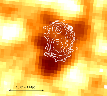
Figure 6.— Planck-reconstructed $Y_{SZ}$ map of G345, overlaid with the XMM-Newton X-ray isointensity contours. Although we see a clear offset of $\sim 10^{\prime}$ between the X-ray and the Sunyaev-Zel’dovich signal peaks, this is consistent with Planck’s much courser spatial resolution and noise, compared to Chandra.

To estimate the expected integrated Compton parameter, we used the electron density and temperature profiles we determined for both subclusters to estimate the electron pressure which we integrate along the line of sight, $P=n_{\rm e,N}kT_{\rm e,N}+n_{\rm e,S}kT_{\rm e,S}$, where the indices N and S correspond to G345N and G345S. The centers of the subclusters are separated by 400 kpc on the sky to match the X-ray observations. We computed the integrated Compton parameter over a sphere of 1260 kpc (the $r_{500}$ given by the Planck Collaboration) centered between the two subclusters (the resulting 2D map is presented in Figure 7). The Planck Collaboration et al. (2011) determines the integrated Compton parameter within $5r_{500}$ to be $Y_{5R_{500}}=1.81Y_{500}$, where $Y_{500}$ is the integrated Compton parameter within $r_{500}$. Using the X-ray derived parameters for the gas temperature and density, we computed a $Y$ Compton parameter of $Y=0.0136\pm 0.0011\rm~{}arcmin^{2}$, which is consistent within $\sim~{}0.8\sigma$ of the Planck Collaboration measured value of $Y=0.0109\pm 0.0032\rm~{}arcmin^{2}$.

We also modified the pressure model from the universal profile (Arnaud et al., 2010) that was used to compute $Y$ by the Planck Collaboration to a two component model that keeps the relative amplitude of the two components fixed to our X-ray model. Using the Matched Multi Filters extraction algorithm, we obtained $Y=0.0119\pm 0.0025\rm~{}arcmin^{2}$, which is consistent within $\sim~{}0.6\sigma$ of our X-ray measured value. This value is also consistent with the previous Sunyaev-Zel’dovich signal measured assuming a universal pressure profile.

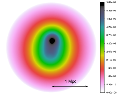
Figure 7.— 2.52 Mpc $\times$ 2.52 Mpc image of the spherically integrated Compton parameter $Y$ with 1 kpc $\times$ 1 kpc resolution. The values are in units of arcmin². The centers of the subclusters were separated by 400 kpc on the sky to match the X-ray observations. We see that most of the Sunyaev-Zel’dovich signal comes from the northern component, since its gas density (and therefore pressure) is considerably higher than that of G345S.

7. A dynamical model for the G345 System

In this section we apply the dynamical model presented by Beers et al. (1982) to the G345N and G345S system to evaluate the dynamical state of the subclusters.

For the case where the subclusters are gravitationally bound, we write the equations of motion in the following parametric form:

$$R=\frac{R_{\rm m}}{2}(1-\cos\chi),$$ (17)

$$t=\left(\frac{R_{\rm m}^{3}}{8GM}\right)^{1/2}(\chi-\sin\chi),$$ (18)

$$V=\left(\frac{2GM}{R_{\rm m}}\right)^{1/2}\frac{\sin\chi}{(1-\cos\chi)},$$ (19)

where $R_{\rm m}$ is the separation of the subclusters at maximum expansion, $M$ is the total mass of the system, and $\chi$ is the development angle used to parametrize the equations. For the case where the subclusters are not gravitationally bound, the parametric equations are:

$$R=\frac{GM}{V_{\infty}^{2}}(\cosh\chi-1),$$ (20)

$$t=\frac{GM}{V_{\infty}^{3}}(\sinh\chi-\chi),$$ (21)

$$V=V_{\infty}\frac{\sinh\chi}{(\cosh\chi-1)},$$ (22)

where $V_{\infty}$ is the asymptotic expansion velocity. The radial velocity difference, $V_{r}$, and the projected distance, $R_{p}$, are related to the system parameters by

$$V_{\rm r}=V~{}\sin\alpha,~{}R_{\rm p}=R~{}\cos\alpha.$$ (23)

The total mass of the system is $M=(4.03\pm 0.33)\times 10^{14}~{}M_{\odot}$ (sum of the masses of both subclusters within $r_{200}$). We assume that the subclusters’ velocities are the line of sight velocities of their central dominant galaxies. We take $R_{\rm p}$ = 0.4 Mpc, the projected distance on the plane of the sky between the dominant galaxies of each subcluster (see Figure 1). The redshift difference between these galaxies yields a radial velocity difference of $V_{r}=1134\pm 66{\rm~{}km~{}s^{-1}}$ (the giant elliptical in G345N is ESO 187-G026, at $z=0.047176\pm 0.000143$, and in G345S the giant elliptical is ESO 187-IG025 NED04, at $z=0.043223\pm 0.000180$, Smith et al., 2004). We close the system of equations by setting $t$ = 12.86 Gyr, the age of the Universe at the redshift of these clusters ($z=0.045$). These equations are then solved via an iterative procedure, which determines the radial velocity difference $V_{\rm r}$ as a function of the projection angle $\alpha$.

Simple energy considerations specify the limits of the bound solutions:

$$V_{\rm r}^{2}R_{\rm p}\leq 2GM~{}{\sin^{2}\alpha\cos\alpha}.$$ (24)

Figure 8 shows the projection angle $\alpha$ as a function of the radial velocity difference $V_{\rm r}$ between the subclusters. The uncertainties in the measured line-of-sight velocity and total mass of the system lead to a range in the solutions for the inclination angles ($\alpha_{\rm inf}$ and $\alpha_{\rm sup}$). The relative probabilities of these solutions are then computed by:

$$p_{i}=\int_{\alpha_{{\rm inf},i}}^{\alpha_{{\rm sup},i}}\cos\alpha~{}d\alpha,$$ (25)

where the index $i$ represents each solution. Finally, the probabilities can be normalized by $P_{i}=p_{i}/(\sum_{i}p_{i})$.

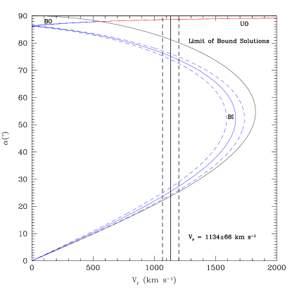
Figure 8.— Projection angle $\alpha$ as a function of the radial velocity difference $V_{\rm r}$ between the subclusters. BO, BI, and UO stand for Bound Outgoing, Bound Incoming, and Unbound Outgoing solutions, respectively. Solid blue and red lines correspond to bound and unbound solutions, respectively. The vertical solid line corresponds to the radial velocity difference between the giant ellipticals. Dashed lines correspond to 68$\%$ confidence ranges.

The radial velocity difference of the subclusters $V_{r}=1134\pm 66{\rm~{}km~{}s^{-1}}$ yields two bound solutions and one unbound solution for $\alpha$. For the bound solutions, the subclusters are either approaching each other at 1173 km s^-1 (17$\%$ probability) or at 2636 km s^-1 (83$\%$ probability). The former solution corresponds to an encounter in less than 1.2 Gyr, given their separation of $\sim$ 1.56 Mpc. The latter corresponds to an encounter in less than 170 Myr, given their separation of $\sim$ 440 kpc. The unbound solution (0.05$\%$ probability) corresponds to a separation of $\sim$ 17 Mpc. These solutions are presented in Tables 7 and 8. Given its low probability, the unbound solution can be neglected, while the bound solution in which the separation between the clusters is $\sim$ 440 kpc is highly favored ($83\%$ probability).

We note, that the dynamical analysis method from Beers et al. (1982) assumes a purely radial infall (no angular momentum). Also, the way the probabilities are computed favors small angle solutions. The small angle bound solution ($25.48^{\circ}$) is highly favored ($P=83\%$) compared to the other bound solution ($75.13^{\circ}$ – $P=17\%$), despite its supersonic infalling velocity ($\sim 2600\rm~{}km~{}s^{-1}$ – the sound speed of a 3 keV cluster is $\sim 900\rm~{}km~{}s^{-1}$, therefore $2600\rm~{}km~{}s^{-1}$ corresponds to a Mach number of $\sim$ 3). The virial radius of these subclusters is roughly 1.2 Mpc. If, indeed, they were separated by only $\sim$ 440 kpc, moving at $\sim 2600\rm~{}km~{}s^{-1}$, shock discontinuities in the X-ray surface brightness would be seen in the region between their cores. Furthermore, fitting the spectrum in a rectangular region (105 kpc $\times$ 345 kpc) between the subclusters gives ${\rm k}T=3.30_{-0.53}^{+0.84}$ at 68% confidence, providing no evidence of shock heated gas between the subclusters. In this analysis, the probabilities for the bound solutions should be treated with caution, as we have no information about the angular momentum of this system.

Table 7Best Fit Parameters for the Bound Incoming Solutions of the Dynamical Model.

$\chi$	$\alpha$	$R$	$R_{\rm m}$	$V$	$P$
(rad)	(degrees)	(kpc)	(kpc)	($\rm km~{}s^{-1}$)	($\%$)
4.952	75.13	1559.5	4089.6	1173.1	17
5.600	25.48	443.1	3952.9	2635.6	83

Note. — Columns list best fit for the $\chi$ and $\alpha$ for the bound solutions of the dynamical model, and the corresponding values for $R$, $R_{\rm m}$, $V$, and probability of each solution.

Table 8Best Fit Parameters for the Unbound Outgoing Solution of the Dynamical Model.

$\chi$	$\alpha$	$R$	$V$	$V_{\infty}$	$P$
(rad)	(degrees)	(kpc)	($\rm km~{}s^{-1}$)	($\rm km~{}s^{-1}$)	($\%$)
3.157	88.67	17213.7	1134.1	1041.5	0.05

Note. — Columns list best fit for the $\chi$ and $\alpha$ for the unbound solution of the dynamical model, and the corresponding values for $R$, $V$, $V_{\infty}$, and probability of this solution.

7.1. A Modified Dynamical Model

Since the Beers et al. (1982) dynamical model is based on the timing argument (see e.g.  Kahn & Woltjer, 1959), which Li & White (2008) have shown to be biased and over-constrained (failing to reproduce the scatter observed in N-body simulations), we also investigate G345 using a modified version of the Dawson (2013) Monte Carlo dynamic analysis method. The Dawson (2013) method relaxes many of the constraints in the timing argument and examines all merger scenarios consistent with the observed state, enabling it to capture the observed scatter in the N-body simulations. Additionally this method models the two subclusters as NFW halos (Navarro et al., 1996) so we can more accurately estimate the time-till-collision ($TTC$), the period between collisions ($T$), and the eventual relative collision velocity ($V_{\rm 3D}(t_{\rm col})$) (for a precise definition of these quantities, please refer to Dawson, 2013). We modified the Dawson (2013) method slightly, since it is designed for post-merger systems and there is strong evidence that G345 is a pre-merger system. We removed the prior that the time-since-collision ($TSC$) be less than the age of the Universe, since $TSC$ is now recast as the $TTC$. We also now allow for unbound scenarios, see Equation (24), however we require that $V_{\rm r}$ be less than the line-of-sight Hubble flow velocity for the unbound realization to be considered valid,

$$V_{\rm r}\leq V_{\rm r,Hubble}=H(\bar{z})R\sin(\alpha),$$ (26)

where $H(\bar{z})$ is the Hubble parameter at the average redshift of the two subclusters. We summarize the results of this analysis in Table 9.

From Figure 9 it can be seen that the large relative velocity and small separation highly favored by the Beers et al. (1982) dynamic model are disfavored by the modified Dawson (2013) dynamic model, as well as being inconsistent with the observed gas properties. However, there are still a number of realizations in the Monte Carlo analysis where effects of the merger on the gas might be expected. In principle these also could be excluded from the posterior distributions. Based on this analysis, we find that the subclusters are likely to collide in 0.5 $\pm$ 0.2 Gyr with a relative collision velocity of 2000 $\pm$ 100 km s^-1, see Figure 10. Based on this dynamic analysis, there is a slightly larger probability (2.6% vs. 0.05%) that the subclusters are unbound, but this scenario is still unlikely. The unbound parameter estimates are also summarized in Table 9.

Table 9Parameter Estimates from Modified Dawson (2013) Dynamics Analysis

Parameter	Units	Bound Scenarios ($\mathcal{L}$=97.4%)			Unbound Scenarios ($\mathcal{L}$=2.6%)
		Location	68% LCL–UCL	95% LCL–UCL	Location	68% LCL–UCL	95% LCL–UCL
M200,N	$10^{14}$ M☉	1.6	1.4 – 1.8	1.1 – 2.0	1.6	1.3 – 1.8	1.1 – 2.0
M200,S	$10^{14}$ M☉	2.5	2.3 – 2.8	2.0 – 3.0	2.5	2.3 – 2.7	2.0 – 3.0
$z_{\rm N}$		0.0472	0.0470 – 0.0473	0.0469 – 0.0474	0.0472	0.0470 – 0.0473	0.0469 – 0.0475
$z_{\rm S}$		0.0433	0.0431 – 0.0434	0.0429 – 0.0436	0.0432	0.0430 – 0.0434	0.0429 – 0.0436
$R_{\rm p}$	Mpc	0.40	0.36 – 0.44	0.32 – 0.48	0.41	0.37 – 0.45	0.33 – 0.50
$\alpha$	degree	59	46 – 70	37 – 77	89	89 – 90	89 – 90
$R$	Mpc	0.81	0.60 –1.3	0.48 –2.0	30	20 – 70	15 – 160
$R_{\rm m}$	Mpc	2.0	1.6 – 2.9	1.4 –5.7	$\cdots$	$\cdots$	$\cdots$
$V_{\rm 3D}(t_{\rm obs})$	km s-1	1300	1200 – 1600	1100 – 1900	1100	1100 – 1200	1000 – 1300
$V_{\rm 3D}(t_{\rm col})$	km s-1	2000	1900 – 2100	1800 – 2300	$\cdots$	$\cdots$	$\cdots$
$TTC$	Gyr	0.5	0.3 – 0.7	0.2 – 1.1	$\cdots$	$\cdots$	$\cdots$
$T$	Gyr	4.9	3.7 –7.8	3.1 – 15	$\cdots$	$\cdots$	$\cdots$

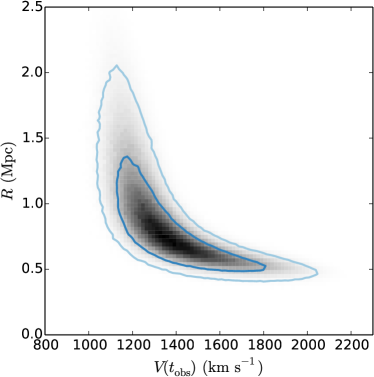
Figure 9.— The marginal posterior of the three-dimensional subcluster separation $d_{\rm 3D}$ and relative velocity $v_{\rm 3D}$ in the observed state $t_{\rm obs}$, inferred from the modified Dawson (2013) dynamics analysis. Dark and light blue contours represent the 68% and 95% confidence regions, respectively.

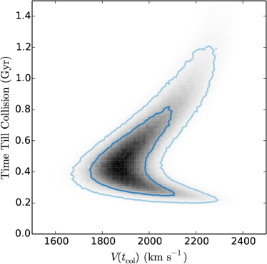
Figure 10.— The marginal posterior of the relative three-dimensional subcluster velocity at the time of collision $v_{\rm 3D}(t_{\rm col})$ and the time it will take to collide given their observed state, inferred from the modified Dawson (2013) dynamics analysis. Dark and light blue contours represent the 68% and 95% confidence regions, respectively.

8. Conclusions

We have presented Chandra, XMM-Newton, and ROSAT observations of G345, a Planck detected double cluster, and provided measurements of temperature, gas and total masses, gas fraction, entropy profiles, expected Sunyaev-Zel’dovich signal, and X-ray luminosities. Both the north and south subclusters have X-ray surface brightnesses that are well described by a $\beta$-model within $r_{500}$, with $\beta\sim 0.5$. Both subclusters have gas masses in the range 1–2 $\times 10^{13}M_{\odot}$ and total masses in the range 1–2 $\times 10^{14}M_{\odot}$, and gas mass fractions in agreement, within the confidence range, of those found by Vikhlinin et al. (2006) for clusters with similar total mass ($0.12\pm 0.02$ for the northern subcluster and $0.09\pm 0.01$ for the southern one). We show that the G345 subclusters that are very likely ($>97\%$ probability) gravitationally bound and infalling and will collide in $500\pm 200$ Gyr. We show that there is good ($0.8\sigma$) agreement between the expected Sunyaev-Zel’dovich signal predicted from the X-ray data and the measured value from the Planck mission, and $0.6\sigma$ agreement when the Planck value is re-computed assuming a two component pressure model, with relative amplitudes fixed using the X-ray results. The high central entropy in G345S can be explained either by the mergers of several groups, as suggested by the presence of five massive elliptical galaxies or by AGN energy injection, as suggested by the presence of a bright radio source in the massive elliptical galaxy ESO 187-IG 025 NED05, or by a combination of both processes.

Appendix A Stellar and Low Mass X-ray Binary Contributions to the X-ray Luminosity of Elliptical Galaxies

A.1. Stellar Contribution

Revnivtsev et al. (2007) showed that the unresolved X-ray halo in M32 can be best explained by the cumulative emission from cataclysmic variables and coronally active stars. In a following work, Revnivtsev et al. (2008) used deep Chandra observations to measure the unresolved X-ray emission in the elliptical galaxy NGC 3379. They suggested that the old stellar populations in all galaxies can be described by a universal value of X-ray emissivity per unit stellar mass or K-band luminosity.

From the 2MASS K-band image of the giant elliptical in G345N (ESO 187-G026), we extract its K-band luminosity and determine its stellar mass. The K-band luminosity measured within 7 kpc from the center of ESO 187-G026 (for comparison with the galaxy’s X-ray luminosity measured within the same region) is $L_{\rm K}=1.6\times 10^{43}\rm~{}erg~{}s^{-1}$. Bell et al. (2003) showed that the relation between the K-band luminosity and the stellar mass is given by:

$${\rm log}\left(\frac{M}{L_{K}}\right)=a_{\rm K}+b_{\rm K}\times(\rm color)$$ (A1)

where the $M/L$ ratio is given in solar units. For the $B-R$ color, $a_{\rm K}$ = -0.264 and $b_{\rm K}$ = 0.138 (Bell et al., 2003). We calculate $B-R$ = 1.63 for ESO 187-G026, which gives $M=1.78\times 10^{11}M_{\odot}$.

The X-ray luminosity in the soft (0.5 – 2.0 keV) band due to stellar emission from ESO 187-G026 can now be computed using the relation given by Revnivtsev et al. (2007):

$$L_{\rm 0.5-2.0~{}keV}=7\times 10^{38}\left(\frac{M}{10^{11}M_{\odot}}\right)\rm erg~{}s^{-1}$$ (A2)

Using Equation (A2) we compute a soft X-ray luminosity of $L_{\rm 0.5-2.0~{}keV}=1.25\times 10^{39}\rm~{}erg~{}s^{-1}$, $\sim$ 0.5 % of the total X-ray emission of the galaxy.

A.2. Low Mass X-ray Binaries

Low mass X-ray binaries (LMXB) also contribute to the unresolved X-ray emission of galaxies. Gilfanov (2004) showed that the distribution of near-infrared light in all galaxies closely traces the azimuthally averaged spatial distribution of LXMBs. To describe it quantitatively, they defined a template for the X-ray luminosity function as a power law with two breaks:

$$\frac{dN}{dL_{38}}=\left\{\begin{array}[]{ll}K_{1}\left(L_{38}/L_{b,1}\right)^{-\alpha_{1}},&\mbox{\hskip 25.6073pt $L_{38}<L_{b,1}$}\\ K_{2}\left(L_{38}/L_{b,2}\right)^{-\alpha_{2}},&\mbox{$L_{b,1}<L_{38}<L_{b,2}$}\\ K_{3}\left(L_{38}/L_{cut}\right)^{-\alpha_{3}},&\mbox{$L_{b,2}<L_{38}<L_{\rm cut}$}\\ 0,&\mbox{\hskip 25.6073pt $L_{38}>L_{\rm cut}$}\\ \end{array}\right.$$ (A7)

where $L_{38}=L_{X}/10^{38}\rm~{}erg~{}s^{-1}$ and normalizations $K_{1},K_{2},$ and $K_{3}$ are related by

$$K_{2}=K_{1}\left(L_{b,1}/L_{b,2}\right)^{\alpha_{2}}$$

$$K_{3}=K_{2}\left(L_{b,2}/L_{\rm cut}\right)^{\alpha_{3}}$$ (A8)

They fixed the value of the high luminosity cut-off at $L_{\rm cut}=500\times 10^{38}\rm~{}erg~{}s^{-1}$. Due to the steep slope of the luminosity function above $L_{b,2}$, the results are insensitive to the actual value of $L_{\rm cut}$. Typically, for nearby galaxies, the source detection threshold defines the luminosity cut-off. However, for ESO 187-G026 we cannot resolve any point sources, so the luminosity cut-off is set to their fixed maximum value of $L_{\rm cut}=500\times 10^{38}\rm~{}erg~{}s^{-1}$.

Gilfanov (2004) provides the best fit value for the average normalization of $K_{1}=440.4$ per $10^{11}~{}M_{\odot}$, and the best fits to the parameters of the luminosity distribution of $\alpha_{1}=1.0$, $\alpha_{2}=1.86$, $\alpha_{3}=4.8$, $L_{\rm b,1}=0.19$, and $L_{\rm b,2}=5.0$.

We can now compute the cumulative number of sources using:

$$N_{\rm X}(>L)=\int_{L}^{L_{\rm cut}}\frac{dN}{dL_{38}}~{}dL_{38},$$ (A9)

and the total luminosity by:

$$L_{\rm X}(>L)=\int_{L}^{L_{\rm cut}}\frac{dN}{dL_{38}}~{}L_{38}~{}dL_{38},$$ (A10)

which yields $L_{\rm 0.5-2.0~{}keV}(>10^{35}\rm~{}erg~{}s^{-1})=1.62\times 10^{40}~{}erg~{}s^{-1}$ for ESO 187-G026. This leads to a (stellar + LMXB) luminosity of $L_{\rm 0.5-2.0~{}keV}=1.74\times 10^{40}\rm~{}erg~{}s^{-1}$, which corresponds to $\sim 7\%$ of the galaxy’s total 0.5–2.0 keV measured X-ray luminosity within 7 kpc of its center.

References

- Abell et al. (1989) Abell, G. O., Corwin, H. G., Jr., & Olowin, R. P. 1989, ApJS, 70, 1
- Anders & Grevesse (1989) Anders, E., & Grevesse, N. 1989, Geochim. Cosmochim. Acta, 53, 197
- Andrade-Santos et al. (2012) Andrade-Santos, F., Lima Neto, G. B., & Laganá, T. F. 2012, ApJ, 746, 139
- Andrade-Santos et al. (2013) Andrade-Santos, F., Nulsen, P. E. J., Kraft, R. P., et al. 2013, ApJ, 766, 107
- Arnaud et al. (2010) Arnaud, M., Pratt, G. W., Piffaretti, R., et al. 2010, A&A, 517, A92
- Beers et al. (1982) Beers, T. C., Geller, M. J., & Huchra, J. P. 1982, ApJ, 257, 23
- Beers et al. (1990) Beers, T. C., Flynn, K., & Gebhardt, K. 1990, AJ, 100, 32
- Beers et al. (1992) Beers, T. C., Gebhardt, K., Huchra, J. P., et al. 1992, ApJ, 400, 410
- Bell et al. (2003) Bell, E. F., McIntosh, D. H., Katz, N., & Weinberg, M. D. 2003, ApJS, 149, 289
- Bîrzan et al. (2008) Bîrzan, L., McNamara, B. R., Nulsen, P. E. J., Carilli, C. L., & Wise, M. W. 2008, ApJ, 686, 859
- Bock et al. (1999) Bock, D. C.-J., Large, M. I., & Sadler, E. M. 1999, AJ, 117, 1578
- Buote & Tsai (1996) Buote, D. A., & Tsai, J. C. 1996, ApJ, 458, 27
- Cavagnolo et al. (2009) Cavagnolo, K. W., Donahue, M., Voit, G. M., & Sun, M. 2009, ApJS, 182, 12
- Cavagnolo et al. (2010) Cavagnolo, K. W., McNamara, B. R., Nulsen, P. E. J., et al. 2010, ApJ, 720, 1066
- Cavaliere & Fusco-Femiano (1976) Cavaliere, A., & Fusco-Femiano, R. 1976, A&A, 49, 137
- Dawson (2013) Dawson, W. A. 2013, ApJ, 772, 131
- Dawson (2014) Dawson, W. A. 2014, Astrophysics Source Code Library, 7004
- Douglass et al. (2011) Douglass, E. M., Blanton, E. L., Clarke, T. E., Randall, S. W., & Wing, J. D. 2011, ApJ, 743, 199
- Forman & Jones (1982) Forman, W., & Jones, C. 1982, ARA&A, 20, 547
- Gilfanov (2004) Gilfanov, M. 2004, MNRAS, 349, 146
- Jeltema et al. (2005) Jeltema, T. E., Canizares, C. R., Bautz, M. W., & Buote, D. A. 2005, ApJ, 624, 606
- Jones & Forman (1984) Jones, C., & Forman, W. 1984, ApJ, 276, 38
- Jones & Forman (1999) Jones, C., & Forman, W. 1999, ApJ, 511, 65
- Kahn & Woltjer (1959) Kahn, F. D., & Woltjer, L. 1959, ApJ, 130, 705
- Laganá et al. (2010) Laganá, T. F., Andrade-Santos, F., & Lima Neto, G. B. 2010, A&A, 511, A15
- Li & White (2008) Li, Y.-S., & White, S. D. M. 2008, MNRAS, 384, 1459
- Maughan et al. (2012) Maughan, B. J., Giles, P. A., Randall, S. W., Jones, C., & Forman, W. R. 2012, MNRAS, 421, 1583
- Mazzotta et al. (2004) Mazzotta, P., Rasia, E., Moscardini, L., & Tormen, G. 2004, MNRAS, 354, 10
- McDonald et al. (2013) McDonald, M., Benson, B. A., Vikhlinin, A., et al. 2013, ApJ, 774, 23
- Mohr et al. (1995) Mohr, J. J., Evrard, A. E., Fabricant, D. G., & Geller, M. J. 1995, ApJ, 447, 8
- Navarro et al. (1996) Navarro, J. F., Frenk, C. S., & White, S. D. M. 1996, ApJ, 462, 563
- O’Sullivan et al. (2011) O’Sullivan, E., Giacintucci, S., David, L. P., et al. 2011, ApJ, 735, 11
- Revnivtsev et al. (2007) Revnivtsev, M., Churazov, E., Sazonov, S., Forman, W., & Jones, C. 2007, A&A, 473, 783
- Revnivtsev et al. (2008) Revnivtsev, M., Churazov, E., Sazonov, S., Forman, W., & Jones, C. 2008, A&A, 490, 37
- Richstone et al. (1992) Richstone, D., Loeb, A., & Turner, E. L. 1992, ApJ, 393, 477
- Planck Collaboration et al. (2011) Planck Collaboration, Ade, P. A. R., Aghanim, N., et al. 2011, A&A, 536, A8
- Planck Collaboration et al. (2013) Planck Collaboration, Ade, P. A. R., Aghanim, N., et al. 2013, A&A, 550, A132
- Pratt et al. (2010) Pratt, G. W., Arnaud, M., Piffaretti, R., et al. 2010, A&A, 511, A85
- Seigar et al. (2003) Seigar, M. S., Lynam, P. D., & Chorney, N. E. 2003, MNRAS, 344, 110
- Smith et al. (2004) Smith, R. J., Hudson, M. J., Nelan, J. E., et al. 2004, AJ, 128, 1558
- Sun et al. (2007) Sun, M., Jones, C., Forman, W., et al. 2007, ApJ, 657, 197
- Vikhlinin et al. (2001) Vikhlinin, A., Markevitch, M., Forman, W., & Jones, C. 2001, ApJ, 555, L87
- Vikhlinin et al. (2005) Vikhlinin, A., Markevitch, M., Murray, S. S., et al. 2005, ApJ, 628, 655
- Vikhlinin et al. (2006) Vikhlinin, A., Kravtsov, A., Forman, W., et al. 2006, ApJ, 640, 691
- Vikhlinin et al. (2009) Vikhlinin, A., Burenin, R. A., Ebeling, H., et al. 2009, ApJ, 692, 1033
- Vikhlinin et al. (2009) Vikhlinin, A., Kravtsov, A. V., Burenin, R. A., et al. 2009, ApJ, 692, 1060
- Voit et al. (2005) Voit, G. M., Kay, S. T., & Bryan, G. L. 2005, MNRAS, 364, 909
- Wang et al. (2004) Wang, Q. D., Owen, F., & Ledlow, M. 2004, ApJ, 611, 821
- Zel’dovich & Raizer (1967) Zel’dovich, Y. B., & Raizer, Y. P. 1967, New York: Academic Press, 1966/1967, edited by Hayes, W.D.; Probstein, Ronald F.,