The Complex North Transition Region of Centaurus A: Radio Structure

Abstract

We present deep radio images of the inner $\sim 50$ kpc of Centaurus A, taken with the Karl G. Jansky Very Large Array (VLA) at 90 cm. We focus on the Transition Regions between the inner galaxy – including the active nucleus, inner radio lobes and star-forming disk – and the outer radio lobes. We detect previously unknown extended emission around the Inner Lobes, including radio emission from the star-forming disk. We find that the radio-loud part of the North Transition Region, known as the North Middle Lobe, is significantly overpressured relative to the surrounding ISM. We see no evidence for a collimated flow from the Active Galactic Nucleus (AGN) through this region. Our images show that the structure identified by Morganti et al. (1999) as a possible large-scale jet appears to be part of a narrow ridge of emission within the broader, diffuse, radio-loud region. This knotty radio ridge is coincident with other striking phenomena: compact X-ray knots, ionized gas filaments, and streams of young stars. Several short-lived phenomena in the North Transition Region, as well as the frequent re-energization required by the Outer Lobes, suggest that energy must be flowing through both Transition Regions at the present epoch. We suggest that the energy flow is in the form of a galactic wind.

1. Introduction

The radio source Centaurus A (“Cen A”) and its parent galaxy, NGC 5128, form an important active-galaxy system which can reveal the interplay between the history of the parent galaxy and the development of the radio source it creates. Only 3.8 Mpc away, (Harris et al. 2010; $1\arcmin\simeq 1.14$ kpc ), Cen A/NGC 5128 can be studied with a level of detail unavailable in other systems. Interestingly – or perhaps because the system is so close – both the stellar galaxy and the radio source show details that we do not normally expect.

NGC 5128 is fundamentally a normal elliptical galaxy, dominated by an old stellar population with kinematic signatures typical of other massive ellipticals. The galaxy’s optical appearance is, however, somewhat unusual, being dominated by the iconic central dust band, which is thought to be the result of a merger with a smaller gas-rich system. Other remnants of the merger may include cold HI still orbiting the galaxy and a ribbon of young stars and emission-line gas clouds (e.g., Graham 1998, Mould et al. 2000, Struve et al. 2010). In a companion paper (Neff, Eilek, & Owen 2014, Paper 2), we show that ribbon extends to $\sim 35$ kpc from the galaxy, is coincident with a complex, knotty structure seen in radio and X-rays, and is probably energized by a galactic wind moving through the middle regions of the radio source.

Our focus in this paper is the radio structure of the inner $\sim 50$ kpc of Cen A. We present new VLA 90 cm observations, and discuss their implications for the astrophysics of the region and the overall energy flow in the system. In Section 2, we review relevant background information on the Cen A / NGC 5128 system and present a first look at our results. Section 3 describes our radio observations and imaging methods. Section 4 presents our 90 cm image, and discusses its limitations. Section 5 compares our image to the 20 cm results from Morganti et al. , 1999 (“M99”). In Sections 6 and 7, we present and analyze various components of the Inner and Transition regions. In Section 8, we discuss the need for energy flow through the Transition Regions and argue that those regions are dominated by a wind rather than jets. Section 9 summarizes our results.

2. Cen A: Setting the Stage

We begin with the three spatial scales of the system – small, large and intermediate, as summarized in Figure 1 and Table 1 – and continue with an introduction to key aspects of the system. All distances within Cen A are given in projection on the sky.

Figure 1a (from Junkes et al. 1993), shows the entire radio source, including the bright Inner Lobes, the relatively bright North Middle Lobe, and the extended Outer Lobes. We note there is no southern counterpart to the North Middle Lobe. Figures 1b and 1c are from this paper. Most of our focus in this paper is Figure 1b: we present a new look at the base of the North Middle Lobe. Our VLA observations show new detail around the Inner lobes and the base of the North Middle Lobe, leading to a new interpreation of these phenemona. We will present newly detected diffuse emission around the Inner Lobes, including emission from the starburst in the central gas/dust disk in NGC 5128. We see no evidence of the “large-scale jet”, reported by M99 as extending beyond the North Inner Lobe (in Section 5 we compare our results to the M99 image). Because our images beyond the base of the North Middle Lobe are contaminated by emission from the outer lobes, our focus will be on the region shown in Figure 1b.

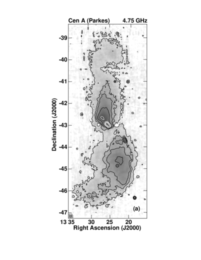
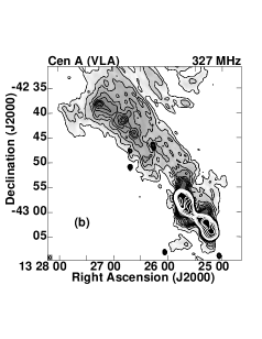
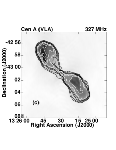
Figure 1.— The three scales of Cen A as seen in radio. Left (a), the large-scale Outer Lobes (also known as “giant” lobes); 5-GHz Parkes image (Junkes et al.   (1993), kindly provided by N. Junkes). Contour levels 0.1, 0.3, 0.5, 1, 3, 10, 30, 60 $\times~{}624$ mJy/beam. Upper Right (b), our 327-MHz image showing 35 kpc of the intermediate-scale North Middle Lobe. Contour levels 6, 8, 10, 12, 14, 16, 18, 20, 40, 70, 100, 200, 400, 700, 1000, 2000 $\times~{}10$ mJy/beam. Lower Right (c), our 327-MHz image of the small-scale, 15-kpc Inner Lobes. Contour levels 1, 2, 4, 6, 10, 20, 40, 60  $\times~{}100$ mJy/beam.

Table 1Specialized acronyms related to Cen A

Acronym	Definition	Scalea
		(kpc)
(N,S)ILs	(North, South) Inner radio Lobes	$\sim 7$, $\sim 5.5$
(N,S)TRs	(North, South) Transition Regions	$10-40$
NMLb	North Middle radio Lobe	$10-40$
(N,S)OLs	(North, South) Outer radio Lobes	$40-300$

^a Spatial scales give approximate distance from AGN, in projection.
^b We use “North Middle Lobe” only when referring to radio emission from the North Transition Region.

2.1. Large scales: the outer lobes

Cen A is perhaps best known for its large-scale, double-lobed, FRI radio source, extending $\sim 600$ kpc end-to-end (Figure 1a, also Junkes et al. 1993, Feain et al. 2011). In addition to being radio-loud, the Outer Lobes are extended $\gamma$-ray sources (e.g., Yang et al. 2012). The North and South Outer Lobes are generally similar, but differ in detail. The North Outer Lobe is straighter and extends $\sim 4.5^{\circ}$ ($\sim 270\arcmin$) on the sky, while the South Outer Lobe bends from south to east and extends $\sim 4^{\circ}$ ($\sim 240\arcmin$).

The Outer Lobes are relatively old. Eilek (2014; “E14”) argues, based on dynamical models, that the age of the large-scale radio structure is on the order of 1 Gyr and is no younger than $\sim 400$ Myr old. Because this age is much greater than the radiative lifetimes of electrons in the Outer Lobes (at most $\sim 80$ Myr for radio-loud electrons, and only $\sim 1$ Myr for the electrons creating the $\gamma$-rays by inverse Compton scattering of the Cosmic Microwave Background Radiation; e.g., E14), it is clear that the outer lobes are not “dead”. Rather, they must have been energized quite recently in order to keep shining, especially in $\gamma$-rays. E14 argues that MHD turbulence within the lobes can provide the necessary in situ energization, but that the turbulence itself will decay in no more than $\sim 30$ Myr unless it is resupplied from the Active Galactic Nucleus (AGN). Thus, the outer lobes cannot have been disconnected from any driver for more than a few tens of Myr.

2.2. Small scales: the AGN and the central galaxy

The inner few kpc of the galaxy contains two sources of power, both of which are quite young compared to the $\sim$Gyr age of the outer radio lobes.

The massive black hole in the nucleus of NGC 5128 is active right now, driving out pc-scale jets (e.g., Muller et al. 2011). Plasma from the nuclear jets accumulates in two inner radio lobes, which extend $\sim 7$ kpc NE and $\sim 5.5$ kpc SW of the radio core (Figure 1c). The northern jet can be traced continuously in radio (Burns et al. 1983) and X-rays (Schreier et al. 1981) from the galactic core out to $\sim 5$ kpc, where it bends, loses collimation, and expands to create the North Inner Lobe (NIL). No kpc-scale jet has been found in the South Inner Lobe (SIL), although a few compact knots SW of the core may indicate an unseen jet (Goodger et al. 2009), and filamentary structure within the SIL suggests an ordered flow.

X-ray observations show that NGC 5128’s interstellar medium (ISM) is disturbed by, and interacting with, the radio jet and Inner Lobes. Two X-ray bright patches (Kraft et al. 2007) suggest an interaction of the North Inner Lobe with the local ISM, and a discontinuity in X-ray emission appears to coincide with the jet decollimation (Kraft et al. 2008). To the south, X-ray images show the expanding South Inner Lobe is driving a shock into the ISM. Because the shock strength can be related to the expansion speed of the South Inner Lobe, these data show that the Inner Lobes are only a few Myr old (Section 8.1, also Croston et al. 2009).

A starburst is currently underway in the core of NGC 5128. The central, warped gas and dust lane contains young stars (e.g., Dufour et al. 1979), young clusters (Minitti et al. 2004), and HII regions (Bland et al. 1987), all of which indicate ongoing active star formation in the disk. This starburst has continued for at least 50 Myr, and probably longer. In Paper 2 we argue the starburst and AGN together are driving a wind which carries energy into and through the middle regions of the radio source.

2.3. Intermediate scales: the transition regions

Our focus in this paper is the regions between the inner and outer radio lobes. We refer to these regions, $\sim$10$-$40 kpc north and south of the galaxy, as the North and South Transition Regions (NTR, STR).

Radio emission in the transition regions

To the north, low-resolution radio images (e.g., Figure 1a, from Junkes et al. 1993; also Hardcastle et al. 2009) show a conspicuous bright structure that appears to connect the north end of the North Inner Lobe to the inner part of the North Outer Lobe. This structure extends to at least $\sim 40$ kpc from the active core of NGC 5128 and is the region of highest radio surface brightness after the inner lobes. It is situated where the larger-scale radio source gradually bends from the NE orientation of the northern jet and North Inner Lobe, towards the NW and thence into the North Outer Lobe. This structure is known as the North Middle Lobe in the literature, and we follow that tradition in this paper when we refer to the radio-loud part of the North Transition Region. Figure 1b shows our new 90-cm image, which we discuss in detail in Section 6.

No comparable feature exists to the south; there is no “South Middle Lobe”. Junkes et al. (1993) detect a diffuse bridge of faint radio emission connecting the South Outer Lobe to the core and South Inner Lobe, $\sim 10$ times fainter surface brightness than the corresponding region to the north. This diffuse emission is resolved out in higher-resolution radio images (e.g., Feain et al. 2011, also our new images in Section 6).

M99 explored the North Middle Lobe at higher resolution ($56\arcsec\times 30\arcsec$). Their 1.4-GHz image shows a quasi-linear structure, which starts at the outer edge of the North Inner lobe, extends $\sim 10$ kpc to the NE, and then broadens out to make up part of the diffuse structure known as the North Middle Lobe. M99 referred to the linear structure as a “large-scale jet”, to distinguish it from the few-kpc inner jet, but also emphasized that its true nature is unclear. We discuss this linear feature, which we do not see in our images, at length from an imaging point of view in Section 5 and from the point of view of the energy flow in Section 8.3.

X-ray-loud ISM

The quiescent ISM of NGC 5128 can be traced to $\sim 30$ kpc from the galaxy, both to the NW and the SE (e.g., Feigelson et al. 1981, Kraft et al. 2009; “K09”). An X-ray “hole” north of the galaxy (Kraft, 2009) appears to be coincident with the NML, suggesting that radio-loud plasma has created a cavity in the ISM of NGC 5128 similar to those seen in other radio galaxies. Feigelson et al. (1981) found an X-ray ridge near the SE edge of the North Middle Lobe, close to the apparent boundary between the hot, thermal ISM of the galaxy (SE of the ridge) and the nonthermal plasma of the NML (NW of the ridge). XMM-Newton observations (K09) show that the X-ray ridge contains several compact, X-ray-loud knots. In Section 7.2 we show this knotty X-ray ridge is closely related to the radio-bright ridge we describe in Section 6.

“Weather” in the north transition region

In addition to the unusual radio and X-ray emission, the North Transition Region contains a string of optical emission-line filaments and recently formed stars (Graham & Price 1981, Graham 1998, Mould et al. 2000, Crockett et al. 2012). In Paper 2 we show that the emission line region extends to $\sim 35$ kpc from the center of the galaxy, and this structure is also detected in H$\alpha$ and Far-UV emission. By analogy to terrestrial weather, where memorable events (e.g., tornadoes and cyclones) can be dramatic local consequences of atmospheric flows, we refer to this complex mixture of radio and X-ray emission, disturbed multiphase ISM, and star formation as the “weather system.” We explore this system in greater detail in Paper 2.

2.4. Models for the transition regions

The astrophysics of the transition regions is not well understood. The radio loudness of the North Middle Lobe and the emission line filaments in the North Transition Region have received the most attention to date.

Radio loudness of the North Middle Lobe

Although a number of models have been advanced to explain the radio-loudness and structure of the NML, none has emerged as definitive, and none explains all aspects of the region.

Several authors have argued that the linear feature seen by M99 is, indeed, a steady jet which extends past the northern edge of the North Inner Lobe and creates the North Middle Lobe. Junkes et al. (1993) suggested the NML is the region where a large-scale jet first loses energy and creates an expanding plasma cloud. Romero et al. (1996) suggested the NML is a “working surface” where a supersonic jet bends as it runs into the local ISM. Gopal-Krishna and Wiita (2010) suggested that the NML results from an interaction between a jet and gas clouds associated with a stellar shell. All of these suggestions are challenged by our lack of detection (at 90 cm) of a narrow collimated jet within the NML region.

Another common theme holds that the North Middle Lobe was created by a time-variable active nucleus. Saxton et al. (2001) model the NML as a buoyant plasma bubble, formed by a previous outburst of the central radio jet, which has pulled a stream of plasma from the north inner lobe as it rises. Similarly, K09 argue that a bubble was created in an earlier activity cycle, and the bubble is now being energized by plasma outflow from the current AGN outburst and thus seen as the radio-loud NML. These models are challenged by the disparity between the long time necessary for the slowly-rising bouyant bubble to reach the North Transition Region ($\sim 140$ Myr, Saxton et al. 2001) and the many short-lived features seen in the region (as we describe in Section 8.2).

The “missing” South Middle Lobe

We have found surprisingly little discussion of the north-south asymmetry of the middle-scale regions. Haynes et al. (1983) pointed out that relativistic beaming could cause a radio asymmetry, but did not comment on why such beaming would not also affect the inner lobes. Hardcastle et al. (2009) argued that the absence of a bright South Middle Lobe means there is currently no energy flow into the South Outer Lobe. This argument is challenged, however, by the ongoing re-energization required to keep the South Outer Lobe shining in $\gamma$-rays and high-frequency radio emission (e.g., E14). We note that a useful model of the source must explain the brightness difference between the North and South Transition Regions, as well as clarify other features in the northern weather system.

Star formation and emission line filaments

There is a general consensus in the literature that an outflow, usually presumed to be from the AGN, is causally related to the emission-line clouds and young stars in the weather system. Several authors have argued that the narrow feature seen by M99 is a collimated jet which has energized the emission-line clouds and/or induced star formation within the NE weather system. Models include weak shocks in dense clouds photoionizing the ambient gas (Sutherland et al. 1993), or shocks causing cloud fragmentation and collapse with subsequent star formation (e.g., Fragile et al. 2004, Croft et al. 2006). These models for the weather system are challenged by the apparent lack of a jet in the region, as well as by substantial distance offsets of the emission line features from the putative outer jet. However, we will argue that many effects attributed to a jet-cloud interaction can equally well be caused by a wind-cloud interaction. In Paper 2 we return to the galactic wind and explore its likely connection to weather in the North Transition Region, and to differences between the North and South Transition Regions.

3. Observations, Reduction and Imaging

Motivated by the M99 results, we wanted to obtain a better image of the linear feature in their image, which was suggested as a possible large-scale jet. The relatively faint radio emission outside the inner double is difficult to image at 20 cm or shorter wavelengths, because of the extremely bright inner lobes and core. We therefore observed at 90 cm, where we expected the diffuse emission and possible outer jet to be brighter and the central double to be less dominant.

Table 2Observing Runs Summary

Configuration	Date	Time on-source
		(hours)
BnA	2005 January 23	3.28
BnA	2005 January 25	3.28
BnA	2005 February 03	3.31
BnA	2005 February 12	3.27
CnB	2005 June 21	3.28

Table 3Images of Centaurus A at 90 cm

Image	Restoring beam	total flux	rms	Figures	Note
	B${}_{maj}\times$ B${}_{min}\times$ P.A.	(Jy)	( mJy/beam)
Middle Lobes:
combined model	$28\arcsec\times 17\arcsec\times 11^{\circ}$	1389	3.0	—	(a)
convolve35	$35\arcsec\times 25\arcsec\times 0^{\circ}$	1389	5.3	2,3
convolve40	$40\arcsec\times 30\arcsec\times 0^{\circ}$	1389	7.2	—	(c)
High Pass Filtered	$40.0\arcsec\times 30.0\arcsec\times 0.0^{\circ}$	723	–	7, 8	(d)
Inner Double
combined model	$21.5\arcsec\times 11.4\arcsec\times 3.5^{\circ}$	991	3.7	—	(a)
convolve22	$22\arcsec\times 12\arcsec\times 0^{\circ}$	991	4.4	6(a)	(b)
convolve25	$25\arcsec\times 20\arcsec\times 0^{\circ}$	991	8.0	6(b)	(b)
ATCA 21 cm	$60.5\arcsec\times 36.25\arcsec\times 2.88^{\circ}$	46	5.4	4, 5	(e)
Matched VLA 90 cm	$60.5\arcsec\times 36.25\arcsec\times 2.88^{\circ}$	624	28	4, 5	(e)

(a) Image is weighted average of images made for each of the 4 band/polarization combined-day datasets.
(b) Restoring beams used for images and measurements are indicated in captions.
(c) Image used as starting point for High-pass filtered image.
(d) Open-filtered image, made from image with restoring beam $40\arcsec\times 30\arcsec\times 0^{\circ}$, to highlight structure on scales less than $\sim 2.7\arcmin$.
(e) ATCA image kindly provided by R. Morganti. Matched VLA 90 cm image convolved to identical resolution. Neither of these images contain all of the inner double source; total fluxes indicate what is in the images and do not measure the source’s total flux density.

We observed with the VLA in BnA, and CnB configurations for a total of 16.4 hours on-source between January and June 2005, as shown in Table 2. We observed mainly at night, to avoid ionospheric phase destabilization and to minimize radio interference from terrestrial orgins. Observations were centered on the active nucleus, at J2000.0 coordinates 13^h25^m27.6^s, -43^∘01′09″. The VLA was tuned to two bands centered at 321.5 and 327.5 MHz; each band received both left-circular and right circular polarization, giving us a total of four band/polarization (“band/pol”) pairs. Data from each band/pol pair were collected in spectral line mode, with 15 channels covering a bandwidth of 5.86 MHz, for a total bandwidth of 11.7 MHz. The narrow individual channel observations helped avoid bandwidth smearing of regions away from the field center (beam smearing increases linearly as a function of distance from the field center and at $30\arcmin$ from the center is $\sim 2\arcsec$, very much less than our synthesized beam), and also proved helpful in excising Radio Frequency Interference (RFI).

3.1. Calibration & Editing

All reductions were done using the Astronomical Imaging Processing System (AIPS) package (Greisen 2003). For each day’s observation, we first split a bright point source calibrator from the raw database and applied a phase self-calibration. Then we used this otherwise uncalibrated source to calculate a bandpass correction which was used to flatten the spectral response. After initial examination of the data, one channel in the lower band was deleted from all data because of persistent strong RFI. The data were calibrated in the standard way, using the AIPS task SETJY with 3C286, and assuming the VLA-determined 1999.2 flux scale. An initial data flagging pass was run to remove obvious RFI.

3.2. Imaging & Self-calibration

Each of the four combinations of band and polarization, on each of the five observation days, was treated separately. We made three or four passes through each data set, with a sequence of imaging (CLEAN algorithm), flagging for RFI, and self-calibration. For these iterations, we imaged a single field $68\arcmin$ across.

Because radio emission from the North Middle Lobe is very low surface brightness, we were concerned that our imaging might be corrupted by nearby sources in the sidelobes of the primary beam. To counter this possible problem, we subtracted our source model for Cen A from the visibility data, and made a large mosaiced image extending to $4^{\circ}$ from the pointing center. (For comparison, the FWHM of the primary beam of a VLA antenna is $\sim 2.25^{\circ}$ at 90 cm, or a radius of $\sim 1.1^{\circ}$). We CLEANed each facet of this mosaic to remove all small-scale sources outside the central $\sim 17\arcmin$. A bright radio galaxy, MRC1318-434B (at $13^{\rm h}21^{\rm m}15^{\rm s}$, -43^∘41′21″) was imaged and removed from the visibility data; other sources were faint and most were unresolved. After the confusing sources were subtracted, the Cen A source model was added back into the visibility data. A few compact sources remained in the central field, projected on or embedded in the Cen A radio emission, and are visible in our images.

The complicated structure with the bright inner lobes proved too complex for a good restoration with the clean algorithm, as we have found for other complex sources such as M87. We therefore moved to the Maximum Entropy (MEM) algorithm implemented in the AIPS program VTESS (Cornwell & Evans, 1985), in order to produce a higher-fidelity image of the diffuse emission from the NML.

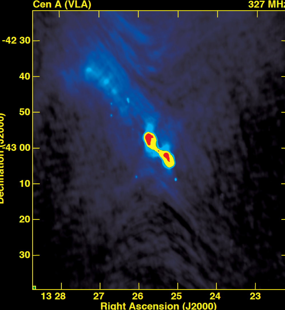
Figure 2.— Our full-field VLA image at 90 cm/327 MHz, covering the NTR and STR regions in addition to bright inner lobes. Diffuse emission is apparent throughout the northern half of the image, comprising the base of what has been called the North Middle Lobe (NML). No comparable emission is seen to the south. Three bright radio knots occur along a faint ridge of emission, both embedded in a broader region of more diffuse emission. We see no indication of a large-scale jet. Emission is also detected beyond the previously-known edges of the inner radio lobes (see Figure 6). Refer to Figure 3 for details of features we believe to be real and/or spurious. The restoring beam for this image is $35\arcsec\times 25\arcsec\times 0^{\circ}$.

We continued with several further cycles of MEM imaging and self-calibration using the MEM model. Final images were produced using VTESS. The four band/pol combinations were each imaged separately, combined with appropriate weighting and convolved with a beam just slightly larger than the fits to the individual dirty beams (array response functions). Two images were produced from the final calibrated data: one of a larger field including the full region occupied by the North Middle Lobe and any southern counterpart, the other focusing on the central double source and inner jet. The images were corrected for the primary beam response of the telescopes. Table 3 lists the properties of the final images used in the paper.

We also produced a spatially filtered image following the method of Rudnick (2002), to help in the analysis of small-scale structures within the North Middle Lobe, without contamination form the diffuse background emission We used the AIPS task MWFLT to produce an “open” filtered image, which contains all emission from structures larger than $\sim 2.7\arcmin$. The open filtered image was then subtracted from the original image, leaving only emission from scales smaller than $\sim 2.7\arcmin$ in the high-pass filtered image. We return to this topic in Section 7.

4. Radio structure of the region at 90 cm

In Figure 2 we show the inner $\sim 90$ kpc of Cen A. The bright inner lobes are clearly seen, although overexposed. The broad, diffuse emission to the NE is the base of the North Middle Lobe as seen at 90 cm. In the top panel of Figure 3 we present the same image, but with a deeper stretch, and we label significant features in our image which we believe are real and which are discussed in detail later in the paper. These figures reveal key points about the region.

$\bullet$ We detect diffuse emission outside of, but close to, the Inner Lobes which has not been reported before. As indicated in the top panel of Figure 3, we see emission extending north from the outer edge of the North Inner Lobe. We also detect extended emission almost perpendicular to the Inner Lobes. We call this latter region “the ruff” and we suggest it is radio emission from the star-forming disk. We discuss these features in more detail in Section 6.2.

$\bullet$ In agreement with previous, lower-resolution work (Section 2.3), we detect the base of the North Middle Lobe as a broad, diffuse structure, extending $\sim 10-40\arcmin$ ($\sim 11-45$ kpc) from the North Inner Lobe to the lower region of the North Outer Lobe. It has a well-defined edge to the SE, in agreement with the 20-cm image from M99. The SE edge is roughly coincident with the NW edge of the X-ray emission from the galactic ISM; as noted above (Section 2.3), this edge is probably where the thermal ISM abuts the nonthermal plasma in the North Transition Region. We discuss this diffuse emission further in Section 6.3.

$\bullet$ We see no evidence for collimated outflow beyond the North Inner Lobe as suggested by M99. We do, however, see diffuse emission extending directly north from the North Inner Lobe which blends into the general North Middle Lobe. We also see a relatively bright, curved line of emission, which contains three bright radio knots; we refer to this feature as the “ridge” or “knotty ridge”. Both of these features are labelled in the top panel of Figure 3. The south end of the knotty ridge overlaps the north end of the linear feature identified by M99. This structure lies close to the SE edge of the North Middle Lobe. We discuss it further in Section 7, and we show in Paper 2 that it is spatially coincident with the complex ribbon of optical emission lines, young stars, Far-UV, and X-ray emission which we call the weather system.

$\bullet$ We do not detect any emission from the South Transition Region, down to our sensitivity limit. As previous authors have noted, while faint diffuse emission does exist in this region, (e.g., Junkes et al. 1993), there is no strong southern counterpart to the North Middle Lobe.

4.1. Limitations of our observations

There are particular challenges to observing a source so far south with the VLA. The source is never more than $12^{\circ}$ above the horizon; at very low elevations the VLA antennas shadow one another and/or pick up interfering signals from foreground telescopes; loss of coherence due to the ionosphere is exacerbated at low elevations. Given the difficulties inherent in these observations, we identify several effects which may affect image quality, as follows.

Contamination by emission from the outer lobes.

All of the structures presented here, including the inner and transition regions of Cen A, are embedded in much larger ($\sim 8^{\circ}$) outer lobes. Because the outer lobes are introduced into the imaging through the outer parts of primary beam, they can appear as peculiar structures in the images. We suspect this is the cause of some of the noticeable artifacts in our images, which we were unable to remove. However, the signatures of these artifacts are readily recognized and thus unlikely to be mistaken for source structures (as discussed in Section 4.2).

Primary beam effects.

The shape of the 90 cm response from VLA antennas is asymmetric and does not fall to a full null; rather the sensitivity falls off gradually for many degrees. In addition, the primary beam is not circularly symmetric, which causes structures far from the field center to be modulated as the parallactic angle changes. Because the Outer Lobes of Cen A are bright at 90 cm, significant brightness on large scales will be detected in the outer parts of the primary beam, which cannot be fully removed due to the modulation. This large-scale, sidelobe-detected emission, collected from an asymmetric beam pattern, appears in the images as low-level texture in the image background.

Limited uv coverage.

The arrays we used for these observations are sensitive to structures of size up to $\sim 1.25^{\circ}$. The field that was imaged is $\sim 2^{\circ}$, in each dimension, but the largest images of the North Middle Lobe shown in this paper are $\sim 1^{\circ}$ across. Therefore, the structures we show and discuss are not affected by missing short uv spacings. However, we are unable to image larger-scale emission, because we do not have data sensitive to the scales of the outer lobes, as well as the other issues with the Outer Lobes discussed above. Further, the images are affected by missing uv samples at certain angles in the outer part of the uv-plane, which arise because of the low declination and limited viewing time of the source.

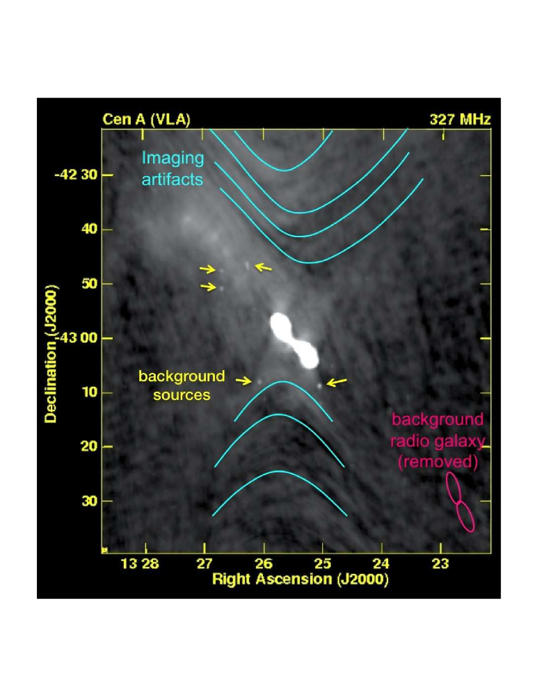
Figure 3.— Lines overlaid on our full-field, 327-MHz image showing which features are where, and indicating their reality (or not). Upper figure, what we believe: in addition to extended diffuse emission from the North Middle Lobe, we detect a knotty ridge towards the SE edge of the North Middle Lobe, and extended emission close to, but outside of, the Inner Lobes. Lower figure: imaging artifacts, as discussed in Section 4.2, and background sources. This is the same image as in Figure 2, with a different stretch. The restoring beam is $35\arcsec\times 25\arcsec\times 0^{\circ}$.

Imaging a large field.

Because the MEM algorithm implemented in AIPS (or CASA) does not allow mosaicing of multiple fields on a correct 3D grid, we could not account for the curvature of the sky near the edges of the large image. Point sources will be noticeably distorted and therefore poorly represented beyond a distance of $\sim 0.3^{\circ}$ from the field center, and emission on scales $\sim 1\arcmin$ will be affected if it is further from the field center than $\sim 0.7^{\circ}$. We addressed the possible issue for small sources by making a multifaceted image and subtracting the point sources found further than $\sim 8\arcmin$ from the field center, as described in section 2.2. We avoided problems possibly affecting larger structures by imaging fields smaller than the scales that would be affected.

4.2. Artifacts in our image

In the lower panel of Figure 3 we indicate schematically which features in the image we do not believe. The V-shaped dark gaps swooping across the field, and the parallel stripes extending diagonally from SW to NE roughly parallel to the North Middle Lobe’s structure, are very likely artifacts of the image reconstruction, due to the low elevation and resultant foreshortened visibility of Cen A when viewed from the VLA. We also do not believe the dark gap on the NW edge of the North Middle Lobe is physical. Based on previous observations (as mentioned in Section 2.3), we think it likely that the diffuse, North Middle Lobe emission continues smoothly to the north, becoming fainter as as it merges into the northern outer lobe and fades below our detection limits. The mottling seen in the background of Figure 3 probably results from sidelobe detections of the bright Outer Lobes.

5. Comparison to Morganti (1999)

Our 90-cm JVLA image of the North Middle Lobe is significantly different from the 20-cm image from the Australia Telescope Compact Array (ATCA), presented by M99. In Figure 4 we show both images, side by side, to highlight the similarities and differences. The images are convolved to the same resolution and show identical fields. The stretch for the 20-cm image was chosen to approximate the figures in M99 and to avoid showing unphysical areas of negative flux.

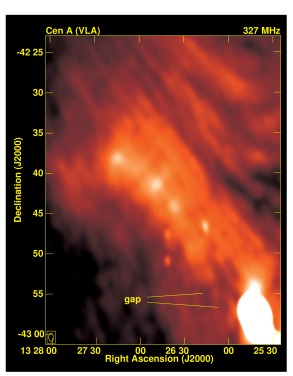
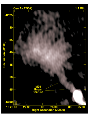
Figure 4.— The North Middle Lobe, as seen by the VLA at 90 cm (left), and by ATCA at 20 cm (right; image kindly provided by R. Morganti). Both images have a beam $60.5\arcsec\times 36.25\arcsec\times 2.88^{\circ}$. This comparison shows that the string of bright knots can be seen at 90 and 20 cm, as can the diffuse emission to the NE of the bright ridge. However, the linear structure connecting the North Inner Lobe to the North Middle Lobe in the 20-cm image is not seen at 90 cm; instead we see a gap just north of the North Inner Lobe, past which the radio ridge begins.

Although there are broad similarities between the two images, they disagree in several details. Both images detect extended diffuse emission from the North Middle Lobe, but that emission is much more extended in our 90-cm image than it is in the 20-cm ATCA image. Our 90-cm image shows no sign of the quasi-linear feature, immediately beyond the edge of the North Inner Lobe, which is seen in the 20-cm image. Instead, our image actually shows a gap – a region of faint but non-zero emission – at the same location as the inner part of the linear 20-cm feature. We also see a broad band of emission extending directly north from the North Inner Lobe and connecting to the broad NML emission. Going outwards, the 90-cm knotty ridge can be seen out to $\sim 30\arcmin$ from the nucleus, after which it bends to the east and disperses. By contrast, the linear structure in the 20-cm image is difficult to follow beyond $\sim 15$′  from the nucleus; past there it disappears into the North Middle Lobe. Looking inwards, the ridge in our 90-cm image does not appear to connect the North Middle Lobe to the North Inner Lobe, but appears instead to bend slightly toward the south and then fade out. The north end of the linear M99 feature can be seen in our observations, but only as a faint enhancement within a much larger region of bright, diffuse emission.

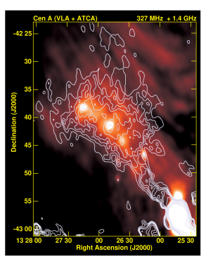
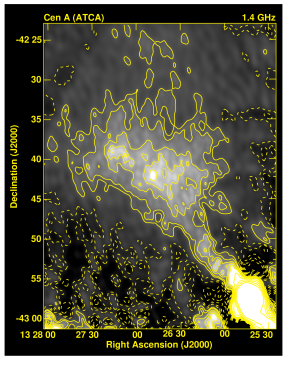
Figure 5.— Comparing the North Middle Lobe at 20 and 90 cm. Left: contours from 20-cm ATCA image (from R. Morganti) overlaid on our 90-cm VLA image. This shows the relation of the linear M99 feature to the broad band of emission, and the string of bright knots, apparent in our 90-cm image. Contour levels are 1, 2, 3, 4, 6, 8, 16, 32, 64, 128 $\times 12.5$ mJy/beam. Right: the 20-cm ATCA image, showing regions of positive and (unphysical) negative flux. Contour levels are -8, -6, -4, -2, -1, 1, 2, 4, 6, 8, 18, 32, 64, 128 $\times 12.5$ mJy/beam; dotted contours show negative fluxes. Both images have the same beam as in Figure 4. $60.5\arcsec\times 36.25\arcsec\times 2.88^{\circ}$.

In Figure 5 we further compare the two images. In the left panel of Figure 5 we show 20-cm contours overlaid on our 90-cm image. This shows that the linear M99 feature lies to the east of the broad emission band we detect at 90 cm, and directly on top of the gap in the 90-cm emission. This figure also shows that the M99 feature appears to connect directly to the knotty ridge we see in the 90-cm image. In the right panel of Figure 5 we show the 20-cm image with stretch and contours chosen to display negative as well as positive fluxes. This figure reveals strong negative fluxes in the 20-cm image on either side of the linear M99 feature. We particularly note a deep negative hole immediately north of the North Inner Lobe, at the point where we see a bright 90-cm feature (labelled “diffuse emission” in Figure 3) which forms the base of the broad emission band to the north.

In the rest of this section we discuss possible reasons for the differences between these two images.

5.1. Observing and imaging differences

Differences in the telescope responses of the VLA and the ATCA are likely to be important in the differences between the way diffuse, relatively faint, emission is detected in our images and those of M99. In particular, accurate detection of faint, diffuse emission in the ATCA image may have been hampered by the lower dynamic range of that image. The central radio source is very bright relative to the North Middle Lobe at 20cm, and ATCA is a relatively sparse array, which can make image reconstruction challenging, even when the source is not at extreme elevations.

Clearly the deep negative fluxes in ATCA image (right panel of Figure 5) are unphysical; we note the ratio of the brightest part of the linear feature to the most negative location right next to the linear feature is only $\sim 1.2$. These negative patches may be hiding or confusing detection of diffuse emission in the regions, and make it unclear how to interpret details of the structures in the M99 images.

5.2. Could we see the linear 20-cm feature in our image?

To test this possibility, we measured the brightness of the M99 linear feature to be $\sim 37$ mJy/beam at 20 cm. If the jet has a spectral index $\alpha=0.5$ ($S_{\nu}\propto\nu^{-\alpha}$), it would have a brightness at 90 cm of $\sim 77$ mJy/beam; if $\alpha=1.0$ it would have a 90-cm brightness of 160 mJy/beam. For comparison, the rms in this part of our 90-cm image is $\sim 50$ mJy/beam. Thus, if the M99 linear feature has $\alpha=0.5$, it would have S/N $\sim 1.5$ in our image, i.e., would be essentially undetectable. If it has $\alpha=1.0$, if would have S/N $\sim 3$ in our image, which would be marginally detectable. Thus, if the linear M99 feature is a physically real feature, it must have a relatively flat spectrum in order to not be detected in our 90-cm image.

We were not able to construct a meaningful spectral index image due to the differing spatial scales sampled and to different noise levels in the two images. However, by averaging many pixels together, we were able to estimate the spectral index in some regions. Within a region coincident with the M99 linear feature, we estimate the spectal index to be $\alpha\sim 0.7$. This rough calculation is consistent with our estimates above: the linear M99 feature may have a flat enough spectral index that most of its length is not detectable above the noise in our 90-cm image. By comparison, the Inner Lobes have spectral indices $\alpha=0.35-0.59$ (Clarke et al. 1992b).

5.3. Missing diffuse flux in ATCA image?

Another striking difference between our 90-cm image and the 20-cm ATCA image is the lack of diffuse flux to the west of the 20-cm linear feature in the ATCA image.

Could this be because the ATCA observations were not sensitive to the diffuse structure? Our observations included uv spacings both smaller and larger than those corresponding to the maximum/minimum ATCA baselines used to produce the image shown in the right panel of Figure 4. The 90-cm observations are sensitive to emission on scales up to $\sim 1.25^{\circ}$, whereas the ATCA observations were sensitive to structures $\>\hbox{\lower 2.5pt\hbox{$\buildrel<\over{\sim}$}}\>25\arcmin$ in size. Because the extended emission we detect from the North Middle Lobe is $\sim 10\arcmin$ across, it should have been visible to the ATCA array. We checked this by making uniform-weighted images (to match M99) from our 90-cm VLA data, while restricting the uv ranges to those available in the two ATCA configurations used in M99. The resulting images still showed extended emission well beyond that seen in M99. Thus, we would have expected ATCA to be sensitive to diffuse emission to the west of the linear feature.

Could the large-scale diffuse emission be too faint for the ATCA to detect at 20 cm? A typical 90 cm brightness level away from the ridge in the North Middle Lobe, sampled with a beam $135\arcsec\times 75\arcsec$ (the restoring beam in the ATCA low-resolution image from M99) is $\sim 1$ Jy/beam. If the extended source has a typical spectral index $\alpha\sim 0.7$, then the expected brightness in the ATCA low-resolution image (with rms level $19$ mJy/beam) would be $\sim 360$ mJy/beam. A similar comparison for the high-resolution ATCA image from M99 (with a $56\arcsec\times 36\arcsec$ beam and rms noise 13 mJy/beam), and corresponding flux $\sim 250$ mJy/beam at 90 cm, implies a brightness $\sim 90$ mJy/beam expected in the 20 cm ATCA image. Therefore, we expect the diffuse emission would have been detectable in the ATCA images if it were there at 20 cm, and if $\alpha\sim 0.7$. The spectral index of the diffuse emission would need to be steeper than $\alpha\sim 1.6$ for the 20cm emission to be below the detection level of the ATCA image.

To summarize, we suspect that low-level diffuse emission in the south of the ATCA image has been confused by the strong negative components of the restored ATCA beam. However, it is also possible that the diffuse emission has a much steeper spectrum than the linear M99 feature, or that it is extremely smooth and thus resolved out by the ATCA observations.

5.4. Foreground absorption from the galaxy?

Finally, we check whether the absence of the linear M99 feature in our image could be due to a forergound absorbing cloud. Such a cloud in the ISM of NGC 5128 might cause the apparent gap in the 90-cm image, where the linear 20-cm should be seen. The recent detection of an HI cloudlet, $\sim 11$ kpc from the galaxy (Struve et al. 2010) and spatially coincident (in projection) with the linear 20-cm feature and 90-cm gap, suggests that associated ionized hydrogen might be absorbing the signal. To check this, we use the expression for free-free absorption, $\tau_{\nu}\simeq 82.T^{-1.35}\nu_{GHz}^{-2.1}n_{e}^{2}L_{kpc}$ for a cloud of electron density $n_{e}$ and thickness $L$. We take the characteristic size of the hole as $L\sim 10$ kpc. The most favorable case for detectable absorption is a cloud at $T\sim 10^{4}$K. In order for such a cloud to be opaque at 327 MHz and transparent at 1.4 GHz, its density must lie in the range $n_{e}^{2}\sim 30-600$ cm^-6 and its pressure in the range $\sim(1.4\!-\!7.0)\times 10^{-11}$dyn cm^-2 ($\sim 16\!-\!80$ times that of the ISM (Section 6.3) ). Hotter clouds must be at even higher pressures to be opaque at 327 MHz. It may be that such an over-pressured cloud just happens to sit in front of the linear 20 cm feature; but we see no sign of the putative cloud in H$\alpha$ or Far-UV emission (as we show in Paper 2). Thus we judge it unlikely that the 90-cm gap is caused by a foreground absorbing cloud.

5.5. The bottom line: imaging challenges

Our long list of potential problems, both for our images and those of M99, mean the final nature of the North Middle Lobe is not yet completely clear. We believe many of the differences between our images and those of M99 are due to a combination of different telescope and array responses and the difficulties of imaging faint diffuse emission in the presence of strong nearby sources. The differences between the images are probably exacerbated by spectral index variations across the source. The apparent limitations of both images highlight the need for improved imaging of this iconic nearby system.

In terms of the physics of the region, we agree with previous authors (including M99) that the NML is a region of broad, diffuse emission. We caution, however, that the relatively faint, linear M99 feature is not necessarily a physically meaningful “jet”. It appears to be a relatively bright linear feature within a fainter, broad emission region, but detailed interpretion of the 20-cm ATCA image is made difficult by the strong negative patches around the linear feature.

6. Radio emission in the inner and transition regions

In this section we describe and characterize the diffuse emission we detect in the Inner and Transition regions of Cen A. To characterize physical conditions in the region, we derive the diagnostic $p_{min}$: the minimum pressure the emitting region can have and still produce the observed radio power. Although we do not assume $p_{min}$ is the true pressure of the radio-loud region, comparing $p_{min}$ to the ambient pressure (for instance known from X-rays) can shed light on the astrophysics of the region.

6.1. Minimum pressures as a diagnostic

We remind the reader of important uncertanties in the $p_{min}$ calculation. It needs only two observables – the flux and area of the emitting region – but additional assumptions are also required. One is the low-frequency cutoff of the radio spectrum. The literature contains two different choices here. Some authors (following Burbidge 1965 and Pacholczyk 1970; we call this the “BP” method) assume the radio spectrum extends only to the lowest observable frequencies, typically 10 MHz. Other authors, motivated by shock acceleration theory (following Myers & Spangler 1985; “MS” method), assume the radio spectrum extends to much lower frequencies. Because the particle pressure is dominated by the lowest energies in a power law spectrum, the MS method gives larger $p_{min}$ values than does the BP method, usually by a factor of a few in the case of Cen A. Because both methods have been used for Cen A, we calculate $p_{min}$ both ways (in Tables 4 and 6). In our discussion, however, we use only the more conservative $p_{min}$ from the BP method. We relegate the details of both methods to Appendix A, where the key results are equations A6 and A9.

Two further uncertainties can be critical to interpreting the results. The volume filling factor of relativistic plasma, $\phi$, is unknown, and can have any value $0<\phi\leq 1$. Also unknown is the ratio of total particle pressure to that in radiating leptons (the so-called “$k$” factor; e.g., Burbidge 1959, Pacholczyk 1970). We combine both of these uncertainties in one factor, which we call the pressure scaling factor $\eta$, defined in equation A7 for the BP case and equation A10 for the MS case. For likely conditions in Cen A, we can approximate both cases by $\eta\sim\left[{(1+k)/\phi}\right]^{1/2}$.

What values of $\eta$ might we expect? If the source contains only radio-loud leptons – as might, for instance, describe plasma in the radio jet close to the AGN – $k=0$. If the same source is also uniformly filled, $\phi=1$, then $\eta$ reaches its minimum, $\eta=1$. Alternatively, we know $k\simeq 100$ for galactic cosmic rays, which are dominated by relativistic baryons. Because the radio-loud plasma we detect in the Transition Regions of Cen A is probably drawn from the inner ISM of the galaxy, $k\gg 1$ might be more appropriate there. In addition, although a uniformly filled volume is possible, internal filamentation or geometries such as an outer shell of emission can give $\phi\ll 1$. Both $k>1$ and $\phi<1$ combine to give the pressure scale factor $\eta>1$; for instance, if $k\sim 100$ and $\phi\>\hbox{\lower 2.5pt\hbox{$\buildrel<\over{\sim}$}}\>1$ (as suggested by the observed filamentation in the inner lobes, Clarke et al. 1992b) we might have $\eta$ on the order of $\sim 10$.

In this paper, we formally keep $\eta$ as an unknown parameter, but constrain it where possible from the data. On larger scales, we show in Section 6.2.2 that $\eta\sim 10$ is consistent with pressure balance in the Inner Lobes. In Section 6.3 we show that if plasma in the North Middle Lobe is similar to that in the Inner Lobes – if it also has $\eta\sim 10$ – then the North Middle Lobe must be at higher pressure than its surroundings.

6.2. The Inner Lobe region

Figure 6a shows our high resolution, 90 cm image of the inner $\sim 15$ kpc of Cen A, displayed to show the well-known bright features in the North Inner Lobe and South Inner Lobe. Figure 6b shows the same field, but with the display stretched to emphasize diffuse emission we detect past the sharp edges of the Inner Lobes.

6.2.1 Inner lobe morphology

The morphology of the Inner Lobes in our image is very similar to that seen at 18 cm and 6 cm (Burns et al. 1983, Clarke et al. 1992b). Both Inner Lobes have sharp boundaries, and are much brighter than the more diffuse emission farther north in the North Middle Lobe. There is no indication of a violent ”breakout” around the North Inner Lobe at the location of the base of the linear M99 feature (as might be expected if that feature were a jet extending beyond the Inner Lobe). The northern inner jet is clearly visible, extending out from the AGN, flaring out and decollimating at $\sim 4.2\arcmin(\sim 5$ kpc) from the core. We confirm previous results in not detecting any southern kpc-scale jet within the South Inner Lobe.

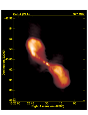
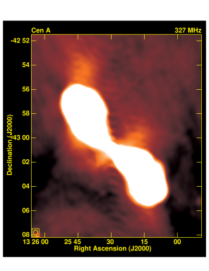
Figure 6.— The Inner Lobes as seen at 327 MHz. The left panel shows the previously known NIL and SIL; structure is very similar to that seen at higher freqencies (1.5 and 5GHz, see text) and here. The image is slightly convolved to $22\arcsec\times 12\arcsec\times 0^{\circ}$. The right panel is a highly stretched image, convolved to $25\arcsec\times 20\arcsec\times 0^{\circ}$ to show the diffuse emission detected beyond the previously known boundaries of the inner lobes. We believe the bright “ruff”, roughly perpendicular to the inner jet, is related to star formation in the galaxy disk. Extended diffuse emission is also seen to the N, and SE of the North Inner Lobe, and to the S of the South Inner Lobe.

Table 4 Synchrotron Analysis for Inner Lobes and North Transition Region

Region	Flux	Area	geometry	distancea	volume	Figure	$p_{min}^{BP}$	$p_{min}^{MS}$
	(Jy)	(amin2)		(amin)	(amin3)		(dyn/cm2)b	(dyn/cm2)b
Inner lobes:
entire NIL	380	15.1	ellipsoid	$\sim$3	34.3	9a	$1.3\eta\times 10^{-11}$	$2.9\eta\times 10^{-11}$
NIL, outer aret	338	10.1	sphere	$\sim$4.5	24.3	9b	$1.5\eta\times 10^{-11}$	$3.3\eta\times 10^{-11}$
entire SIL	282	15.8	ellipsoid	$\sim$3	38.8	9c	$1.0\eta\times 10^{-11}$	$2.4\eta\times 10^{-11}$
SIL, inner part	97	2.41	sphere	$\sim$2	2.81	9d	$2.5\eta\times 10^{-11}$	$5.4\eta\times 10^{-11}$
SIL, outer part	94	3.93	sphere	$\sim$ 4.5	5.87	9e	$1.6\eta\times 10^{-11}$	$3.6\eta\times 10^{-11}$
Near, but outside Inner Lobess:
local region #1	2.73	28.8	pencil beam c	$\>\hbox{\lower 2.5pt\hbox{$\buildrel<\over{\sim}$}}\>6$	$288$	10f	$8.5\eta\times 10^{-13}$	$2.2\eta\times 10^{-12}$
local local region #2	5.21	32.5	pencil beamc	$\>\hbox{\lower 2.5pt\hbox{$\buildrel>\over{\sim}$}}\>8$	$325$	10g	$1.2\eta\times 10^{-12}$	$3.0\eta\times 10^{-12}$
The NML:
Kraft comparison, cylinder	112	350	cylinder	$\sim$20	3670	10a	$4.5\eta\times 10^{-13}$	$1.2\eta\times 10^{-12}$
Kraft comparison, pencil	112	350	pencil beamc	$\sim$20	5250	10a	$3.6\eta\times 10^{-13}$	$1.0\eta\times 10^{-12}$
full NML, ellipsoid	394	2060	ellipsoid	$\sim$35	61,700	10c	$1.8\eta\times 10^{-13}$	$3.5\eta\times 10^{-13}$
full NML, pencil	394	2060	pencil beamc	$\sim$35	32,900	10c	$2.7\eta\times 10^{-13}$	$7.5\eta\times 10^{-13}$
Diffuse, outer, west	20.2	62.6	pencil beamc	$\sim$23	941	10d	$3.7\eta\times 10^{-13}$	$1.0\eta\times 10^{-12}$
Diffuse, inner, saddle	56.9	220	pencil beamc	$\sim$12	3290	10e	$3.2\eta\times 10^{-13}$	$9.0\eta\times 10^{-13}$

^a Distances are from center of galaxy (radio core) to center of region measured.
^b See Section 6.1 for definition of the pressure scale factor $\eta$. We suggest that $\eta\sim 10$ in the Inner Lobes and in the diffuse North Middle Lobe (Sections 6.2.2 and 6.3.1). See equations (A8, A11) to convert $p_{min}$ to $B_{min~{}p}$.
^c Pencil beam depth, $L$, scaled to $10\arcmin$ for region around inner lobes, (excluding featues identified in Figure 3) and to $15\arcmin$ for diffuse emission in transition regions. (See Section 6.3.2 Other choices for line of sight depth, $L$ give $p_{min}^{BP}\propto 1/L^{.581}$ and $p_{min}^{MS}\propto 1/L^{.540}$.

6.2.2 Inner lobe pressures

We measured radio fluxes in several areas of our image, using the AIPS program BLSUM to select regions within which the flux density was summed. Our results are in Table 4; the selected regions are shown in Figure 9 (online material). To get average values through each inner lobe, we measured the flux within the entire lobe. We treat each lobe as a prolate ellipsoid lying in the sky plane. We also measured fluxes within smaller, brighter areas within each lobe, assuming a spherical geometry to derive the sampled volume.

We find $p_{min}\sim\eta\times 10^{-11}$ dyn cm^-2 in the outer parts of both Inner Lobes, and a bit larger for inner part of the South Inenr Lobe. To compare $p_{min}$ to the pressure of the local ISM, we turn to X-ray data. Croston et al. (2009) estimate $p_{ISM}\sim 1.3\times 10^{-12}$dyn cm^-2 for the ISM $\sim 6^{\prime}$ south of the core (ahead of the X-ray shock which bounds the South Inner Lobe). Kraft et al. (2008) estimate $p_{ISM}\sim 3.0\times 10^{-12}$dyn cm^-2 for the ISM $\>\hbox{\lower 2.5pt\hbox{$\buildrel>\over{\sim}$}}\>3.2^{\prime}$ north of the core. We therefore agree with previous authors (Burns et al. 1983, Clarke et al. 1992b), that minimum pressure in the Inner Lobes is well above that of the ISM, so that the Inner Lobes should be expanding into the ISM.

These results allow us to constrain the pressure factor $\eta$ in the Inner Lobes. If the South Inner Lobe is driving a shock ahead of itself into the ISM, its pressure should be comparable to that in the shock. Croston et al. (2009) find $p_{shock}\sim 1.1\times 10^{-10}$dyn cm^-2; in order to have $p_{min}^{SIL}\>\hbox{\lower 2.5pt\hbox{$\buildrel<\over{\sim}$}}\>p_{shock}$, we require $\eta\>\hbox{\lower 2.5pt\hbox{$\buildrel<\over{\sim}$}}\>10$ in the South Inner Lobe. This value is roughly consistent with our suggestions in Section 6.1 that $k\sim 100$, $\phi\>\hbox{\lower 2.5pt\hbox{$\buildrel<\over{\sim}$}}\>1$ in and beyond the Inner Lobe region.

6.2.3 Extended emission around the Inner Lobes

We detect faint but real radio emission beyond the apparent Inner Lobe boundaries. We have stretched the display in the right panel of Figure 6 to show this clearly, and have indicated the features schematically in the top panel of Figure 3. We see broad, diffuse emission beyond the north edge of the North Inner Lobe, extending into the North Middle Lobe region, but not at the right position angle or sufficiently collimated to be the base of M99’s suggested outer jet. We also see a “ruff” of diffuse emission on either side of the “waist” of the inner lobes, with an extent $\sim 5.3$′($\sim 6$ kpc) from NW to SE of the nucleus. This “ruff” is coincident with the dust lane and appears to be radio emission coming from the star-forming disk. We discuss this further in paper 2. More diffuse emission appears to extend from this ruff and wrap around to the NE, around the edge of the North Inner Lobe. Finally, we also see diffuse emission extending beyond the south end of the South Inner Lobe.

6.3. Diffuse emission in the Transition Regions

In this section we characterize diffuse emission in three regions: within the large-scale North Middle Lobe, close to but outside of the Inner Lobes, and at the location where one might expect a South Middle Lobe. Our measurements and derived pressure estimates are collected in Table 4 and summarized in Table 5.

6.3.1 Diffuse emission within the North Middle Lobe.

Figure 2 shows that the North Middle Lobe seen at 90 cm is a broad, diffuse structure. We see no sign of a collimated jet, but we do see three bright compact knots, close to but inside the SE edge of the NML (explored further in Section 7). While the dark diagonal bands cutting through the North Middle Lobe are probably imaging artifacts (Figure 3), the lack of emission to the SE of the North Middle Lobe agrees with previous authors (e.g., M99) and is likely real. This SE edge is where the radio-loud North Middle Lobe plasma abuts the thermal ISM of the galaxy.

To characterize the diffuse emission in the North Middle Lobe, we measured the flux within several hand-drawn regions. One was a rectangular box, of $6.5^{\prime}\times 21.7^{\prime}$, meant to reproduce the area measured by K09. We also measured two other irregular regions of comparable area. Finally, we measured the total flux from a larger area, meant to include the full North Transition Region, including lower surface brightness areas. All areas are shown in Figure 10, and our results are given in Table 4. To convert to volumes we either assumed ellipsoidal or cylindrical geometry in the sky plane, or a pencil beam, $15\arcmin$ through the source, as appropriate for each measurement. The numerical range seen in Table 4 comes from differences among the measured regions, different assumed geometries, and different assumptions in the minimum-pressure calculations (as in Section 6.1). In Table 5 we extract from this range a “characteristic” $p_{min}$ for the North Middle Lobe, $p_{min}\>\hbox{\lower 2.5pt\hbox{$\buildrel>\over{\sim}$}}\>4\eta\times 10^{-13}$dyn cm^-2.

Table 5 Various pressures in the North Transition Region

Region/object	pressure	reference	comments
	(dyn cm-2)
Around the ILs:
thermal ISM (X-rays)	$\sim 1-3\times 10^{-12}$	Section 6.1	$\sim 3-6\arcmin$ from core
inner diffuse radio	$\>\hbox{\lower 2.5pt\hbox{$\buildrel>\over{\sim}$}}\>\eta\times 10^{-12}$	Table 4	$p_{min}$ from synchrotron
Within the NML:
thermal ISM (X-rays)	$\sim 9\times 10^{-13}$	Section 6.3.1	$\>\hbox{\lower 2.5pt\hbox{$\buildrel<\over{\sim}$}}\>30\arcmin$ to SE
diffuse NML (radio)	$\>\hbox{\lower 2.5pt\hbox{$\buildrel>\over{\sim}$}}\>4\eta\times 10^{-13}$	Table 4	$p_{min}$ from synchrotron
Compact features:
X-ray knots (if thermal)	$\sim 2\times 10^{-11}$	Section 7	see Section 7.2 for alternatives
radio knots (if synchrotron)	$\>\hbox{\lower 2.5pt\hbox{$\buildrel>\over{\sim}$}}\>\eta\times 10^{-12}$	Table 6	$p_{min}$ from synchrotron

Synchrotron-based $p_{min}$ values use the more conservative BP method; see Appendix A. The pressure scaling factor $\eta$ (Section 6.1) may vary with location; we suggest that $\eta\sim 10$ in the Inner Lobes and in the diffuse North Middle Lobe (Sections 6.2.2 and 6.3.1), and that $\eta\sim 10$ is a reasonable assumption for the radio knots (Section 7.2).

To compare this to the local ISM, we need the pressure of the ISM and the likely value of the pressure scale factor $\eta$. For the ISM, we use results from K09, who found $p_{ISM}\sim 8.5\times 10^{-13}$dyn cm^-2 for a wedge of the X-ray halo SE of the radio source out to $\>\hbox{\lower 2.5pt\hbox{$\buildrel<\over{\sim}$}}\>30^{\prime}$. We assume this is the dominant pressure in the region. For the pressure scale factor $\eta$, we noted in Section 6.1 that $\eta$ can be as small as unity. This holds if the radio-loud plasma is homogeneous (filling factor of order unity) and if cosmic-ray baryons provide no more pressure than the radio-loud electrons (unlike the galactic ISM). If $\eta\sim 1$, and if $p_{min}$ is close to the true pressure within the North Middle Lobe (meaning that neither the electrons nor the magnetic field greatly dominate the pressure), then the diffuse North Middle Lobe can be in pressure balance with its surroundings.

However, there may be a good case for expecting a larger value of $\eta$ in the region. We pointed out in Section 6.1 that $\eta\sim 10$ would be expected if the radio-loud plasma contains cosmic ray baryons comparable to those in the ISM (where baryon pressure $\sim 100$ times larger than lepton pressure). Furthermore, in Section 6.2.2 we showed that $\eta\sim 10$ is consistent with pressure balance between the South Inner Lobe and the X-ray-loud shock it is driving into the surrounding ISM. If this larger $\eta\sim 10$ also applies to the radio-loud plasma in the diffuse North Middle Lobe, then the North Middle Lobe is at a substantially higher pressure than the local ISM.

6.3.2 Diffuse emission close to the Inner Lobes.

To describe the diffuse emission close to, but outside of, the Inner Lobes, we measured fluxes in two areas, $\sim 6\arcmin$ and $\sim 8\arcmin$ away from the galaxy (shown in online material in Figure 10). We treated each as a pencil beam, taking the depth along line of sight to be $10^{\prime}(\sim 11$ kpc). We find $p_{min}\sim\eta\times 10^{-12}$dyn cm^-2 for the two regions. Again comparing to ambient ISM pressure (from Table 5), we see that – similarly to the situation in the broader diffuse emission throughout the North Middle Lobe – the plasma in this region around the Inner Lobes is at higher pressure than the local ISM, if the scale factor $\eta\sim 10$.

6.3.3 Non-detection of a South Middle Lobe

We do not detect any emission from the region where we might expect a South Middle Lobe (SML) to be. To determine an upper limit for the radio luminosity of a South Middle Lobe, we measured fluxes in two boxes of the same dimensions as those used for the North Middle Lobe. One box was at the location where we would expect to see a South Middle Lobe, and another well away from that location (shown in Figure 10). In the “off-source” regions, we measured a $1\sigma$ noise level of $2.6$ mJy/beam with a $35\arcsec\times 25\arcsec\times 11^{\circ}$ beam, or 6.1 Jy within the box. We set the detection limit for any SML flux within the North Middle Lobe-equivalent box at $3\sigma\sim 18.3$ Jy. This implies a NML/SML brightness ratio of at least 5-6, in agreement with the observed NML/SML surface brightness ratio $\sim 10$ in the Junkes et al. (1993) 4.8 GHz (6.3 cm) image, which had a $4.3\arcmin\times 4.3\arcmin$ beam.

7. Compact features in the North Middle Lobe

While we see no evidence of a collimated jet past the north edge of the North Inner Lobe, we do detect three compact knots of emission, close to the SE edge of the North Middle Lobe and apparently connected by a fainter, narrow ridge of emission. These features are highlighted in a spatially filtered image shown in Figure 7. The ridge extends $13\arcmin-30\arcmin$ ($\sim 15-34$ kpc) from the galactic core, and the knots occur at distances $21\arcmin-30\arcmin$ ($\sim 24-30$ kpc) from the core. The ridge appears to overlay part of, and to be an extension of, the linear feature reported at 20 cm by M99, and the radio-loud knots are near local maxima in the M99 image (Figures 4, 5).

7.1. Measurements: radio knots

Table 6North Middle Lobe Radio Knot Properties:

Region	RA	Dec	Flux	—-Radiusa—-		$p_{min}^{BP}$	$p_{min}^{MS}$
			(Jy)	(arcsec)	(pc)	(dyn/cm2)b	(dyn/cm2)b
North knot	13h27m14.6s	-42∘38′07″	0.164	36	660	$1.2\eta\times 10^{-12}$	$3.2\eta\times 10^{-12}$
Middle knot	13h26m37.2s	-42∘44′05″	0.210	42	770	$1.1\eta\times 10^{-12}$	$2.9\eta\times 10^{-12}$
South knot	13h26m48.6s	-42∘41′26″	0.136	35	640	$1.2\eta\times 10^{-12}$	$3.0\eta\times 10^{-12}$

^a Spherical geometry assumed for each knot; radii determined as discussed in text.
^b See Section 6.1 for definition of pressure scale factor $\eta$. We suggest that $\eta\sim 10$ in the Inner Lobes and in the diffuse North Middle Lobe (Sections 6.2.2 and 6.3.1), and that $\eta\sim 10$ is a reasonable assumption for the radio knots (Section 7.2).

Measurement of the compact knots and the ridge is complicated by the smooth background emission on which they sit. We therefore measured the properties of the knots in our high-pass filtered image, which removed most of the diffuse background emission, reducing the local background to  $\buildrel<\over{\sim}$  10 percent of the remaining peak knot brightness. Taking the remaining very local background and the ridge emission into account, we measured the knot fluxes and sizes by examining slices across the knots (perpendicular to the ridge; AIPS tasks SLICE and SLICEPL), and deconvolved the restoring beam of the image from the measured knot sizes. The knots are slightly resolved in our observations, with radii (defined as the half-power half-width of the slice) $\sim 0.7$ kpc. We used transverse slices across the ridge, in the high-pass-filtered image (Figure 7), to estimate the full width of the ridge as $\sim 3.4$ kpc. Because we were not able to differentiate clearly between the ridge and similarly scaled filamentary structure that remained after high-pass filtering, we were not able to obtain a robust measurement of the ridge’s flux.

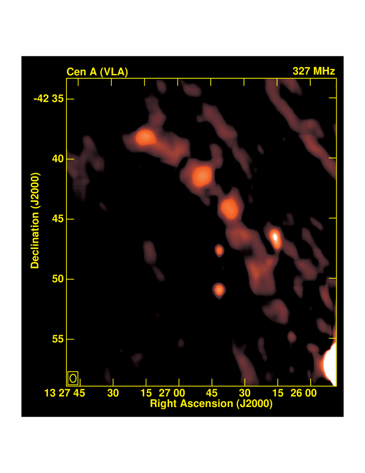
Figure 7.— A spatially filtered version of our 327-MHz image, which highlights the compact features; 3 bright radio knots and the emission ridge which encloses them and extends $\sim 9\arcmin$ ($\sim 10$ kpc) to the SSE. (The three very compact point sources S and W of the radio knots are background sources). Filtering emphasizes emission on $\>\hbox{\lower 2.5pt\hbox{$\buildrel<\over{\sim}$}}\>2.7\arcmin$ scales (Section 3.2 and Table 3). The restoring beam for this image is $40\arcsec\times 30\arcsec\times 0^{\circ}$. The ridge of emission connecting the knots also connects to the linear M99 feature; we believe it is physically real. We suspect other lines to the NW of the knotty ridge are imaging artifacts (Section 4.1 and Figure 3), also highlighted by the algorithm used to create this figure.

Our measured and derived results for the knots are presented in Table 6. Assuming the knots are synchrotron sources, we can derive minimum pressures within the knots, as in Section 6.1. Our measured and derived quantities are given in Table 6; our $p_{min}$ values are summarized in Table 5 and discussed in the next subsection.

We also checked whether the radio knots could be thermal bremsstrahlung sources. If they have the characteristic $\nu^{-0.1}$ thermal spectrum, extrapolating from our 90-cm image predicts the knots should have fluxes $\>\hbox{\lower 2.5pt\hbox{$\buildrel>\over{\sim}$}}\>150-200$ mJy in the 20-cm image from M99. Because this is a factor of 2-3 larger than what is observed, it seems unlikely that the knots are thermal bremsstrahlung sources.

7.2. Comparison: Radio and X-ray knots

The knotty, radio-loud ridge shown in Figures 2 and 7 appears to be closely related to the similar strcture seen in soft X-rays by K09. In Figure 8 we show the relation between the two structures; the X-ray and radio ridges sit almost on top of each other. In the inner part of the ridge, the X-ray and radio knots alternate, with the radio and X-ray knots offset from each other by no more than the diameter of an individual knot ($\>\hbox{\lower 2.5pt\hbox{$\buildrel<\over{\sim}$}}\>1$ kpc). Towards the furthest NE end of the structure, the X-rays bend away from the radio ridge to the east, the separation between the radio and X-ray knots increases, to as much as a few kpc. As noted in Section 2.3, this radio/X-ray ridge is an approximate demarcation between thermal, apparently quiescent galactic ISM east of the North Middle Lobe, and the nonthermal, radio-loud plasma which constitutes the North Middle Lobe and extends to the west of the ridge.

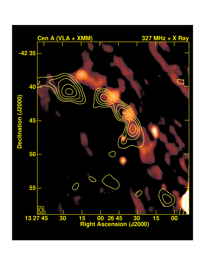
Figure 8.— Relationship between the X-ray knots (yellow contours; from K09) and the radio knots (background image, the high-pass-filtered image from figure 7, beam $40\arcsec\times 30\arcsec\times 0^{\circ}$ ). X-ray data were taken by XMM-Newton and kindly provided by R. Kraft. The inner radio and X-ray knots do not coincide, but rather appear to alternate in a continuous, ridge-like structure.

The radio-loud knots are comparable to the X-ray-loud knots in size and pressure. K09 cite radii $\sim 0.9\arcmin-1.5\arcmin$ for the X-ray knots; we measure somewhat smaller radii, $\sim 0.6\arcmin-0.7\arcmin$ for the radio knots. K09 derive pressures $\sim 1.6-2.4\times 10^{-11}$dyn cm^-2 for the four knots within the X-ray ridge, under the assumption that the X-ray knots are diffuse thermal emission. These pressures are $\sim 20-30$ times higher than that of the galactic ISM ($\sim 9\times 10^{-13}$dyn cm^-2; K09, also Section 6.3.1). We derive minimum pressures $\sim(1.1-1.2)\eta\times 10^{-12}$dyn cm^-2 for the radio knots, under the assumption they are diffuse synchrotron emission. If the pressure scale factor $\eta\sim O(10)$ – as we argue holds for the Inner Lobe and North Middle Lobe region (Section 6.1 and 6.2) – the pressure within the radio-loud knots is significantly higher than that in the nearby ISM and the diffuse North Middle Lobe plasma, and comparable to or larger than that in the X-ray knots.

7.3. Nature of the knots

We do not know the nature of the radio/X-ray knots, but can envision three possibilites.

Extant gas clouds

It may be that both the radio and X-ray knots are simply pre-existing gas clouds

in the region which – for some reason – are radio-loud, X-ray-loud, or both. Although the two sets of knots are not quite spatially coincident, the fact that they have similar sizes and are similarly overpressure with respect to local ISM and to the diffuse North Middle Lobe suggests that the radio knots and X-ray knots may be related phenomena. K09 proposed a pre-existing gas cloud model for the X-ray knots and suggested that a fast plasma flow (such as a jet) from the AGN has heated the clouds to X-ray temperatures. To extend this model to include radio emission one must add additional physics, for instance shocks or turbulence to accelerate locally the relativistic electrons which emit synchrotron radiation. Higher resolution radio and X-ray images could show bow shocks from such a flow.

Multiphase emission-line clouds

In a variant of the previous model, X-ray knots could be hot outer surfaces of multiphase clouds which also produce the ribbon of H$\alpha$ and Far-Ultraviolet emission in this region (Section 2.3, also Paper 2). Similar clouds have been found elsewhere (e.g., the emission-line filaments in M87; Sparks et al. 2010, Werner et al. 2013), and are thought to have a cold interior (H$\alpha$ emission), a warm mid-region (Far-UV emission from CIV lines), and a hot outer layer (X-ray emission from Fe lines). In Cen A, this idea is supported by the X-ray emission which Evans & Koratkar (2004) detected from the inner emission-line filament close to the galaxy. In addition, the X-ray clouds in Cen A have clear internal structure, as might be expected for multiphase ISM clouds (Figures 3 and 5 of K09). Once again, radio emission is not an intrinsic part of this picture, but would have to come from additional physics associated with the cloud’s existence and energization. High-resolution spectral imaging, at X-ray and Ultraviolet wavelengths, could identify and characterize such clouds.

Star formation sites

An alternative possibility is that the radio and X-ray knots are sites of ongoing star formation. This would be consistent with the apparent coincidence of the knots with the extended string of emission-line gas and young stars in the same region (discussed in Paper 2). Although the radio and X-ray knots are larger than “super star clusters” studied elsewhere (typically $\sim 10$ pc across; e.g., Melo et al. 2005 for M82), at least one very young cluster in the Antennae has a radius  $\buildrel>\over{\sim}$  450pc (Whitmore et al. 1999). Interestingly, the luminosities of the knots agree quite well with the lower end of the radio-X-ray relation known to hold for nearby star-forming systems (e.g., Ranalli et al. 2003, Mineo et al. 2014 and references therein). The proxy relations from Ranalli et al. and from Mineo et al. suggest that each knot is currently making stars at $\sim 0.1M_{\sun}$/yr – if the knots are indeed extended star formation sites.

In this picture, the X-rays are not simply from a diffuse gas but rather come from a mix of X-ray binaries and hot plasma (heated by supernovae) in the star-forming region. The nature of the radio emission in this relationship is again unclear, but it is likely to come from relativistic particles accelerated by supernova remnants, possibly supplemented by radio jets driven out from X-ray binaries. If this picture holds, and much of the X-rays or radio emission is not from diffuse plasma, then our minimum pressure estimates of Section 7.1 would not apply. High-resolution space observations, at Ultraviolet and X-ray wavelengths, could identify star-formation sites.

8. Energy Flow in the Transition Regions

Although we have not found clear indications of collimated jets within the North or South Transition Regions of Cen A, power from the inner galaxy must have moved through the Transition Regions in order to create and maintain the Outer Lobes. What can we say about the situation in those regions at present?

8.1. Energy transport on large and small scales

We can probe the situation in the Transition Regions by studying energy flow into and through those regions. Because the Outer Lobes are on the order of a Gyr old, and the current activity cycle of the AGN has lasted only a few Myr, one might expect the time-averaged power needed to create the OLs to be unrelated to the power currently being supplied by the AGN. It turns out, however, that these two powers are quite similar – as we demonstrate here and summarize in Table 7.

AGN power based on radio observations

The energy flowing through the north jet in Cen A can be estimated from high-resolution radio data. Following Owen et al. (2000), the power carried in a jet with radius $r_{j}$, pressure $p_{j}$, density $\rho_{j}$ speed $v_{j}$ and bulk Lorentz factor $\gamma_{j}$ is at least as large as the power being advected out as internal energy: $P_{j,int}\>\hbox{\lower 2.5pt\hbox{$\buildrel>\over{\sim}$}}\>4\pi r_{j}^{2}\gamma_{j}v_{j}p_{j}$. This quantity can itself be limited below by noting that the pressure within the jet is at least that given by the synchrotron mininum pressure, $p_{j}\>\hbox{\lower 2.5pt\hbox{$\buildrel>\over{\sim}$}}\>p_{min,j}$. To estimate the lower limit on $P_{j,int}$ we take take $r_{j}\sim 22$ pc, $v_{j}\sim 0.5c$, from Goodger et al. (2010), and use fluxes those authors measured for the well-resolved knots. Assuming a spectral index $\alpha=0.7$, and guessing that $p_{min}$ across the jet $\sim 1/2$ that in the bright knots, we get a lower limit on the power currently carried by the north jet: $P_{j}\>\hbox{\lower 2.5pt\hbox{$\buildrel>\over{\sim}$}}\>\eta\times 10^{43}$ erg s^-1. In Table 7 we double that to estimate the total power currently being supplied, to north and south, by the AGN.

This estimate of the minimum jet power, today, depends on the unknown pressure scale factor, $\eta$. Although we have argued $\eta$ is of order 10 within the Inner Lobes and the diffuse North Middle Lobe – based on the likely cosmic ray composition of those plasmas – we note that $\eta\>\hbox{\lower 2.5pt\hbox{$\buildrel>\over{\sim}$}}\>1$ could describe an inner jet dominated by relativistic leptons. If this is the case, we have our most conservative lower limit for the jet power currently being created by the AGN, $\>\hbox{\lower 2.5pt\hbox{$\buildrel>\over{\sim}$}}\>2\times 10^{43}$erg s^-1.

Table 7Power estimates for Cen A

Epoch/region	Powera	Timescale
	(erg s-1)	(Myr)
Present-day jets	$\>\hbox{\lower 2.5pt\hbox{$\buildrel>\over{\sim}$}}\>2\times 10^{43}$	today
Recent, over IL life	$\sim(2-6)\times 10^{43}$	$\sim(1-2)$
Historical, over OL lifeb	$\>\hbox{\lower 2.5pt\hbox{$\buildrel>\over{\sim}$}}\>(2\!-\!5)\times 10^{43}$	$\sim(400-600)/\mu$

^a The total power to both sides of AGN, assuming symmetric north and south outflows.
^b The cosine of projection angle between radio lobes and sky plane is $\mu$; $\mu\sim 1/2$ for the inner lobes, but is unknown for the outer lobes.

AGN power based on X-ray observations

The power needed to create the inner radio lobes can be estimated from their impact on the galactic ISM. Croston et al. (2009) used X-ray data to characterize the shock which the South Inner Lobe is driving into the local ISM. That shock is moving in the sky plane at $2600$ km s^-1relative to the ambient ISM. If the ISM is static, the age of the South Inner Lobe is directly found from the shock speed and 5.5-kpc length of the South Inner Lobe (both quantities projected on the sky) as $\sim 2$ Myr. If the ISM is itself in motion (for instance in a fast wind, as we suggest in Paper 2), the South Inner Lobe is younger, perhaps only $\sim 1$ Myr.

Croston et al. (2009) used the shock measurements to estimate the power put out by the AGN over the few-Myr lifetime of the Inner Lobes. They used the shock speed to find the work being done by the inner lobes expanding into the ISM, $pdV/dt\sim 7\times 10^{42}$erg s^-1. This calculation is independent of the age of the South Inner Lobe, but is sensitive to the (unknown) projection angle of the South Inner Lobe. If the South Inner Lobe does not lie in the sky plane, the true shock speed will exceed the measured value, and the rate of work done will be correspondingly larger. Croston et al. (2009) also used the same data to find the enthalpy content of the South Inner Lobe, and from that estimate the power needed to create the South Inner Lobe over an age $\tau_{IL}$ of Myr as $4pV/\tau_{IL}\sim 3\times 10^{43}$ erg s^-1. This estimate is insensitive to the projection angle of the South Inner Lobe, but depends directly on the age; if the South Inner Lobe is younger than 2 Myr, more power is needed. Taking the uncertainties of both estimates into account, we collect the South Inner Lobe-based power estimates as $\sim 1-3\times 10^{43}$erg s^-1, and double that (in Table 7) to estimate the average power supplied by the AGN on both sides over the past few Myr.

Power going into the Outer Lobes

The time-averaged power needed to create the outer lobes can be found from their age and the energy required to expand them to their full size. Following E14, the energy needed to build one of the Outer Lobes is at least $E_{OL}\sim(2-3)\times 10^{59}/\mu$ erg. Unlike the Inner Lobes, we have no information on the projection angle of the outer lobes, so we keep $\mu$, the cosine of that angle, as a variable. The numerical range in $E_{OL}$ allows for uncertainty in the Outer Lobe plasma, which can be internally relativistic or can be dominated by thermal material. If significant internal flows exist today, $E_{OL}$ is greater than this value. The dynamic models presented by E14 show that the age of the Outer Lobes is $\tau_{OL}\sim(400\!-\!600)/\mu$ Gyr; the range of numbers here reflects different possible models.

Putting these results together, we find the time-averaged power $\langle P_{OL}\rangle=E_{OL}/\tau_{OL}$ needed to grow each Outer Lobe, if they contain no significant internal flows, is $\sim(0.95-2.3)\times 10^{43}$ erg s^-1. If significant flows exist within the lobes the necessary power is larger. As with the similar calculation for the Inner Lobes, this estimate is nearly independent of $\mu$. Multiplying this by a factor of two for the two sides of the radio source, we find the average power put out by the AGN over the $\sim$ Gyr lifetime of the source must have been $\>\hbox{\lower 2.5pt\hbox{$\buildrel>\over{\sim}$}}\>(1.9\!-\!4.6)\times 10^{43}$ erg s^-1.

8.2. Short-lived phenomena in and around the North Transition Region

Although we do not know the detailed history of energy transport from the inner galaxy – steady or episodic – we can identify several phenomena which will soon decay or dissipate if they are not maintained by some energy source active today in the North and South Transition Regions.

Diffuse plasma in the North Middle Lobe

We argued in Section 6.3.1 that pressure of the diffuse radio-loud plasma in the North Middle Lobe is likely to be several times larger than that of the quiescent ISM at a comparable distance from the galaxy. Unless the North Middle Lobe is confined by some unseen mechanism (which we judge unlikely), it cannot be a static structure, but should be expanding at approximately its internal sound speed, $c_{s}$. Because we don’t know the thermal plasma content of the North Middle Lobe, we cannot know $c_{s}$, but we can estimate its lower bound. We take the North Middle Lobe pressure as $\>\hbox{\lower 2.5pt\hbox{$\buildrel>\over{\sim}$}}\>p_{min}\sim 4\times 10^{-12}$dyn cm^-2 (from Table 5, taking $\eta\sim 10$ which we argued in Section 6.3.1 is probably the case for the North Middle Lobe as it is for the Inner Lobes). Recalling the hints of an X-ray cavity in the region (Section 2.3), we suggest the density witin the North Middle Lobe is no larger than the ambient ISM density, $\sim 10^{-3}$cm^-3. It follows that the local sound speed $c_{s}=(4p/3\rho)\>\hbox{\lower 2.5pt\hbox{$\buildrel>\over{\sim}$}}\>720$ km s^-1(using mean particle mass $0.6m_{p}$). Taking the characteristic radius of the NML as $\sim 12$ kpc, we expect the North Middle Lobe to expand away in in no more than $\sim 16$ Myr.

Radiative lifetimes in the NML

The North Middle Lobe is detected by the Wilkinson Microwave Anisotropy Probe (WMAP) at frequencies as high as 90 GHz (Hardcastle et al. 2009). Comparison of its flux there to the 5-GHz flux reported by Junkes et al. (1993) shows a relatively flat spectrum between 5 and 90 GHz. Thus the high-frequency radiation cannot simply be the “tail” of a fading electron distribution; we must ask if in situ energization is needed.

Determining the synchrotron age of these electrons is difficult because we do not know the magnetic field in the North Middle Lobe (recall that we do not assume that the minimum-pressure field, from Section 6.1 and Appendix A, measures the true field value). We can, however, find an upper limit to that age. Following E14, let the electrons lose energy only by inverse compton scattering (Stawarz et al. 2006 show that the CMBR dominates galactic starlight at the distance of the North Middle Lobe), until they find themselves in a strong field within the North Middle Lobe. This gives us the largest possible synchrotron life. If we guess that strong field $\sim 10\mu$G (about twice the field at which magnetic pressure balances local ISM pressure – as might be appropriate for shock-enhanced fields within the NML) the maximum lifetime for electrons radiating at $\nu$ is $\sim 180\nu_{GHz}^{-1/2}$ Myr (from E14). This shows that electrons in the North Middle Lobe radiating at $\sim 1-10$ GHz do not require in situ energization, but electrons radiating at 90 GHz will fade in no more than $\sim 20$ Myr without re-acceleration.

Table 8Timescales in the Transition Regions

Object	Timescale	Notes
Diffuse NMLa	$\>\hbox{\lower 2.5pt\hbox{$\buildrel<\over{\sim}$}}\>16$ Myr	overpressure expansion
Synchrotron aging	$\>\hbox{\lower 2.5pt\hbox{$\buildrel<\over{\sim}$}}\>20$ Myr	at/above $\sim 90$ GHz
OL re-energization	$\>\hbox{\lower 2.5pt\hbox{$\buildrel<\over{\sim}$}}\>30$ Myr	turbulent decay in OLs
Radio/X-ray knotsb	$\sim 0.5\!-\!3$ Myr	if diffuse gas clouds
Radio/X-ray knotsc	$\sim 10$ Myr	if star-forming regions

^a Assumes the diffuse North Middle Lobe is at higher pressure than its surroundings (Section 6.3.1).
^b Applies if the radio and X-ray knots are diffuse, unconfined plasma (Section 7.3).
^c Applies if the X-ray knot emission comes from massive young stars (Section 7.3).

Re-energization of the Outer Lobes

The Outer Lobes are much older than the radiative lifetime of their relativistic electrons, especially those detected in $\gamma$-rays (E14, also Section 2.1). They must, therefore, be frequently re-energized. E14 argued this must happen at least every few tens of Myr to maintain the internal turbulence which can re-accelerate the electrons. Because the Transition Regions are the only conduit to the Outer Lobes, it follows that some form of energy transport must have permeated both the North and South Transition Regions at least as recently as $\sim 30$ Myr ago.

Radio and X-ray knots: diffuse gas clouds

In Section 7.3 we noted that the radio and X-ray knots could be either diffuse gas clouds or regions of star formation. If the knots are diffuse gas clouds, they are strongly overpressured, $\>\hbox{\lower 2.5pt\hbox{$\buildrel>\over{\sim}$}}\>20p_{ISM}$. Unless they are somehow confined, they will dissipate quickly. As K09 discuss, if the X-ray knots are unconfined structures with size $\sim 1$ kpc and temperature $T\sim 0.5$ keV, they will expand at their adiabatic sound speed in only $\sim 3$ Myr. For the radio knots, we know the radius ($\sim 0.7$ kpc, Section 7), but – as with the diffuse North Middle Lobe – we do not know their internal sound speed. We therefore find its lower bound by taking the smallest likely pressure and the largest likely density. Let a radio-loud cloud contain plasma at the local ISM density, $\sim 10^{-3}$cm^-3, with pressure $\>\hbox{\lower 2.5pt\hbox{$\buildrel>\over{\sim}$}}\>10^{-11}$dyn cm^-2 (Table 5, taking $\eta\sim 10$). Its sound speed is thus $\>\hbox{\lower 2.5pt\hbox{$\buildrel>\over{\sim}$}}\>1300$ km s^-1. Such a cloud, if unconfined, will last no more $\sim 0.5$ Myr. Thus, if the radio and X-ray knots are separate clouds within the weather system, both will dissipate in no more than few Myr unless they are somehow confined.

Radio and X-ray knots: clumps of young stars

We also noted in Section 7.3 that the X-ray and radio knots may be star-forming regions. If this is the case, the region cannot be age-dated by the the high knot pressures. If the radio and X-ray emission comes from diffuse ISM witin the region, self-gravity of the star cluster and/or wind outflow supplied by the star formation can maintain the high pressures over a longer timescale. However, X-ray emission from star-forming regions can also come from X-ray binaries. Hard X-ray emission comes from high-mass binaries, which only last $\sim 10$ Myr. Because the knots have only been observed at soft X-ray energies (K09), and because soft X-rays can have origins other than high-mass stars, we cannot with certainty state that the radio/X-ray knots contain young stars. However, observational evidence for such young stars elsewhere within the weather ribbon (e.g., Graham 1998, Mould et al. 2000) suggests that similarly young stars might exist within the X-ray/radio knots if they are star-forming regions.

Other short-lived weather in the North Transition Region

The above discussion shows that several features related to the radio and X-ray emission in the Transition Regions probably require re-energization on timescales of a few to a few tens of Myr. We summarize these features in Table 8. In addition, we show in paper 2 that a trail of emission line filaments and young stars stretches $\sim$ 35 kpc outward from the galaxy, along the southeast edge of the North Transition Region. Gas dynamics, cooling times, and stellar ages in this system all indicate timescales no longer than $\sim 10$ Myr.

8.3. Energy flow through the Transition Regions

The power estimates in Table 7 show that the current output of the AGN is sufficient to create and maintain the large-scale radio source, if provided consistently over the $\sim$ Gyr lifetime of the source. This power must have moved outwards, through the North and South Transition Regions, as the Outer Lobes grew to their present size. If the North Transition Region contains such a flow at present, that flow can potentially provide the driver needed for the short-lived phenomena in the region. Although we do not know the history of the AGN, we can consider different possibilities.

An episodic AGN with a low duty cycle?

The youth of the Inner Lobes (only $\sim 1\!-\!2$ Myr old) suggests that power from the AGN has not been steady, but rather has fluctuated with time. How long can the AGN have been “off”? As an example, say the AGN has been quiet for $\>\hbox{\lower 2.5pt\hbox{$\buildrel>\over{\sim}$}}\>30$ Myr (the longest lifetime in Table 8). If remnants of plasma from the previous active cycle of the AGN have been coasting at 3000 km s^-1(the likely deprojected advance speed of the end of the South Inner Lobe; Section 8.1), they would have travelled $\>\hbox{\lower 2.5pt\hbox{$\buildrel>\over{\sim}$}}\>100$ kpc, well past the Transition Regions. Therefore, any material left in the Transition Regions today would be nearly static, and unable to maintain the short-lived phenomena we see in the North Transition Region. We conclude that such a long “down time” for the AGN is unlikely.

An AGN with a high duty cycle?

It may also be that the AGN is “on” for a large fraction of the time, but with a time-variable outflow. It may drive out collimated jets, or a broader diffuse flow, or it may alternate between these two states. If this is the case, plasma in the Transition Regions is probably still in motion, because the flows from the previous active cycle (before the current one that has created the Inner Lobes) have not yet moved through the regions. We find this model attractive – because it does not require us to be catching Cen A at a special time – but we cannot prove it is the case.

We note that the starting plumes which we see as today’s Inner Lobes might evolve in two different ways as they move through the Transition Regions. They may continue to be identifiable as jets, similarly to the inner jets in 3C219 (Clarke et al. , 1992a). If this is the case, Transition Regions will look quite different after $\sim 15$ Myr when the new jets have reached them. Alternately, the Inner Lobes might evolve, via instabilities, into a broader, diffuse flow or turbulent plume, perhaps similar to the rapidly broadening plumes in M84 (e.g., Laing et al. 2011). When these diffuse plumes reach the Transition Regions, they would not necessarily be identifiable as a confined jet, and the Transition Regions would look about the same in $\sim 15$ Myr as they do now.

No jets in the Transition Regions?

Although both our observations and those of M99 detect linear structures near the SE edge of the North Transition Region, which may connect to each other, we do not believe these can be the main source of power for the North Transtion Region or the North Outer Lobe. Our reasoning is as follows.

$\bullet$ Classic jets in well-studied radio galaxies are narrow, well-collimated, continuous outflows which begin at the AGN and carry mass and energy to the large-scale radio lobes. Such a jet clearly exists in the North Inner Lobe of Cen A. It can be traced from the core to $\sim 5$ kpc north, where it bends toward the west and appears to disrupt (Figure 6, also Clarke et al. 1992b). The North Inner Lobe has a sharp northern edge, with no sign of any “jet breakout”, which would be expected if the linear M99 feature were a continuation of the north jet flow currently powering the North Inner Lobe.

$\bullet$ There is no sign of a jet in the South Inner Lobe, although power is very likely being supplied to it at present (evinced by shock expansion, Section 2.2). Furthermore, there is no sign of any collimated flow past the South Inner Lobe, continuing into and through the South Transition Region, although ongoing power is needed to keep the both the South and North Outer Lobes shining in $\gamma$-rays (Section 2.1).

$\bullet$ Although the diverse short-lived phenomena in the North Transition Region need ongoing energization, there is no clear connection between the narrow linear M99 feature, or the knotty ridge we detect at 90 cm, and the broader diffuse North Middle Lobe. As we show in paper 2, the linear M99 feature is also offset from many of the emission-line clouds and young stars in the region, which also need ongoing drivers. It therefore seems unlikely that this faint, narrow feature can drive the entire system.

$\bullet$ By contrast with a jet – a narrow, collimated outflow emanating from the AGN – we envision a “wind” as a more diffuse structure. It can be broader, less well collimated, and may come from a larger region of the galactic core. Well-studied examples (the solar wind, or winds from starburst galaxies) tell us that wind flows can be inhomogeneous, with internal shear surfaces, shocks, and localized high-speed streams. We suspect that the knotty ridge we observe at 90 cm, as well as the linear M99 feature, indicate similar inhomogeneities in a diffuse wind moving through the North Transition Region of Cen A.

9. Final Words

Our new findings, reported in this paper, change and enhance our picture of the North and South Transition Regions in Cen A.

$\bullet$ We see no indication of a large-scale jet in either Transition Region. We do not find any evidence of a radio jet (which we define as a continuous, highly collimated, plasma flow from the AGN) in the middle regions of Cen A. Our observations show the diffuse radio emission known as the North Middle Lobe contains a bright, knotty, emission ridge close to the southeast edge of the region. We suggest that the linear feature reported by M99, and interpreted by many authors as a large-scale jet, is part of this radio ridge. However, the true nature of this region remains elusive, due to technical limitations of existing images. We look forward to future observations with next-generation telescopes which will clarify the structure of the regions.

$\bullet$ Energy must have been moving through both Transition Regions very recently. The energy provided by the current level of nuclear activity, if continually supplied, is sufficient to create and maintain the Outer Lobes over the $\sim$ Gyr lifetime of Cen A. Although we have no direct evidence of plasma flow within the Transition Regions right now, several short-lived structures in the NTR indicate that something must have energized those phenomena on the order of $\sim 10$ Myr ago, if not more recently. The need for ongoing re-energization of the Outer Lobes also shows that energy must have moved through both Transition Regions no more than $\sim 30$ Myr ago.

$\bullet$ Previous models of the North Middle Lobe are inadequate. Many of the models suggested to explain the North Middle Lobe cannot work, because they depend on the existence of a collimated jet passing through the region now. Models which depend on the North Middle Lobe being a slowly rising bouyant bubble have trouble explaining the short-lived phenomena in the North Transition Region and the need for rapid re-energization of both Outer Lobes.

$\bullet$ In Paper 2 we return to the question of energy flow and short-lived phenomena within the Transition Regions. We show that a wind is expected in Cen A/NGC 5128, discuss observational signatures of such a wind, and argue that such a wind naturally explains the enhanced radio emission and other weather phenomena seen in the North Transition Region.

Appendix A Minimum pressure analysis

The energy content in relativistic particles and magnetic fields is a key factor in the physics of synchrotron sources. Because synchrotron power depends on the product of the two, these cannot be determined uniquely from the data, One way to separate particles from fields is to minimize the total pressure, $p_{rel}+p_{B}$, subject to the constraint that the volume emissivity is known (e.g. Burns, Owen & Rudnick 1979). Details matter here; variants of this method found in the literature can be confusing. In this appendix we describe the specific calculations we present in Section 6.

To implement this, we must connect the observed synchrotron power to the total pressure in relativistic electrons. If the electron energy distribution $n(\gamma)$ is defined over some range $\gamma_{1}<\gamma<\gamma_{2}$, the pressure is

$$p_{rel,e}={1\over 3}\int_{\gamma_{1}}^{\gamma_{2}}n(\gamma)\gamma mc^{2}d\gamma$$ (A1)

We assume the usual electron power law, $n(\gamma)\propto\gamma^{-s}$, which produces a power-law synchrotron spectrum, $\epsilon_{sy}(\nu)\propto\nu^{-\alpha}$, where the spectral index $\alpha=(s-1)/2$. The choice of limits in equation (A1) matters because $p_{e}$ is dominated by electrons close to the low-energy cutoff, but radio observations generally do not extend to low enough frequencies to determine this cutoff.

Many authors (e.g, Pacholczyk 1970, Burbidge 1956) choose the range of electron energies corresponding to a specific range of observed radio frequencies, $\nu_{1}<\nu<\nu_{2}$, and assume no electrons radiate outside this range. In principle this frequency range should be chosen based on the broad-band spectrum of a given source, but in practice is typically parameterized as, say, 10 MHz to 10 GHz. Because the electron energy is related to the emitted frequency by $\nu=a\gamma^{2}B$ (for $a=3e/4\pi mc$), the integral in equation (A1) can be written

$$p_{rel,e}={1\over 3}\int_{(\nu_{1}/aB)^{1/2}}^{(\nu_{2}/aB)^{1/2}}n(\gamma)\gamma mc^{2}d\gamma$$ (A2)

With this, the electron pressure, $p_{e}$, is connected to the synchrotron emissivity, $\epsilon_{sy}(\nu_{o})$ at some observed frequency $\nu_{o}$, as

$$p_{rel,e}={1\over 3}{A^{BP}\over B^{3/2}}~{};\quad A^{BP}={\epsilon_{sy}(\nu_{o})\nu_{o}^{\alpha}\over(2\alpha-1)}{2c_{1}^{1/2}\over c_{2}}{\left[1-(\nu_{2}/\nu_{1})^{-(2\alpha-1)/2}\right]\over(\sin\theta)^{3/2}\nu_{1}^{(2\alpha-1)/2}}$$ (A3)

Here $\sin\theta$ is the pitch angle (between particle velocity and magnetic field); $B\sin\theta$ can also be thought of as the projection of the B field on the sky plane. The numerical factors $c_{1},c_{2}$ are given in Pacholczyk (1970). In our calculations we take $\nu_{1}=10$ MHz, and choose $\alpha=0.7$. For this spectral index, the derivations are only weakly sensitive to $\nu_{1}$: $A^{BP}\propto\nu_{1}^{-0.2}$. We also assume $\left[1-(\nu_{2}/\nu_{1})^{-(2\alpha-1)/2}\right]/(\sin\theta)^{3/2}\simeq O(1)$.

An alternative approach was proposed by Myers & Spangler (1985). They argued that the low-energy electron cutoff is set by the physics of the source, not the happenstance of our observations. They treat the low-energy cutoff in the electron energies, $\gamma_{1}$, as an input parameter, and retain the form (A1) in subsequent analysis. To implement this approach, we connect $p_{rel,e}$ to the emissivity as

$$p_{rel,e}={1\over 3}{A^{MS}\over B^{\alpha+1}}~{};\quad A^{MS}={\epsilon_{sy}(\nu_{o})\nu_{o}^{\alpha}\over(2\alpha-1)4\pi c_{5}(\alpha)}{(2c_{1})^{-\alpha}\over(m_{e}c^{2})^{(2\alpha-1)}}{\left[1-(\gamma_{2}/\gamma_{1})^{-(2\alpha-1)}\right]\over\gamma_{1}^{(2\alpha-1)}(\sin\theta)^{\alpha+1}}$$ (A4)

where $c_{5}(\gamma)$ is another constant from Pacholczyk. In our calculations we take $\gamma_{1}=10$, and $\alpha=0.7$. With this spectral index, our calculations are again only weakly dependent on $\gamma_{1}$: $A^{MS}\propto\gamma_{1}^{-0.4}$. We also assume $\left[1-(\gamma_{2}/\gamma_{1})^{-(2\alpha-1)}\right]/(\sin\theta)^{\alpha+1}\simeq O(1)$.

To evaluate $A^{BP}$ or $A^{MS}$, we derive the synchrotron volume emissivity, $\epsilon_{sy}(\nu_{o})$ form the observed flux at $\nu_{o}$ by $\epsilon_{sy}(\nu_{o})=4\pi D^{2}F(\nu_{o})/V_{emit}$, inferring the emitting volume $V_{emit}$ from observations. One immediate uncertainty appears here: the volume inferred from an image, $V_{obs}$, may be incompletely filled, as $V_{emit}=\phi V_{obs}$, with filling factor $\phi<1$. A second uncertainty is how to connect $p_{rel,e}$ to the total plasma pressure, $p_{plasma}$. This quantity can include relativistic baryons and, possibly, other contributions such as thermal plasma. We follow the usual approach by writing $p_{plasma}=(1+k)p_{rel,e}$. We retain both $\phi$ and $k$ as unknown parameters; in our calculations (below) they combine as $(1+k)/\phi$.

Either equation (A3) and (A4) can be used to minimize the total pressure of the magnetized plasma,

$$p_{rel}=p_{plasma}+p_{B}=(1+k)p_{rel,e}+{B^{2}\over 8\pi}$$ (A5)

For the BP method, minimizing equation (A5) with respect to $B$ leads to

$$p_{min}^{BP}={7\over 24}\left[2\pi A^{BP}{(1+k)\over\phi}\right]^{4/7}={7\over 24}\left[2\pi A^{BP}]\right)^{4/7}\eta^{BP}$$ (A6)

where we have defined

$$\eta^{BP}=\left[(1+k)\over\phi\right]^{4/7}$$ (A7)

Also useful relations for the BP case include

$$p_{plasma}={4\over 3}p_{B}~{};\quad B_{min~{}p}^{BP}=\left[2\pi A^{BP}\right]^{2/7}\left[\eta^{BP}\right]^{1/2}$$ (A8)

For the MS method, minimizing equation (A5) with respect to $B$ leads to

$$p_{min}^{MS}={3+\alpha\over 8\pi(1+\alpha)}\left[{4\pi\over 3}(1+\alpha)A^{MS}{(1+k)\over\phi}\right]^{2/(3+\alpha)}={3+\alpha\over 8\pi(1+\alpha)}\left[{4\pi\over 3}(1+\alpha)A^{MS}\right]^{2/(3+\alpha)}\eta^{MS}$$ (A9)

where

$$\eta^{MS}=\left[{(1+k)\over\phi}\right]^{2/(3+\alpha)}$$ (A10)

We again have the useful relations for the MS case,

$$p_{plasma}={2\over 1+\alpha}~{}p_{B}~{};\quad B_{min~{}p}^{MS}=\left[{4\pi\over 3}(1+\alpha)A^{MS}\right]^{1/(3+\alpha)}\left[\eta^{MS}\right]^{1/2}$$ (A11)

For spectral index $\alpha=0.7$, our choice in this paper, the numerical values of $\eta^{BP}=\left[(1+k)/\phi\right]^{0.57}$ and $\eta^{MS}=\left[{(1+k)/\phi}\right]^{0.54}$ are quite similar. In discussion in the paper we drop the “MS” and “BP” superscripts and use the approximate $\eta\sim\left[(1+k)/\phi\right]^{1/2}$ in numerical estimates.

Appendix B Regions where fluxes and areas were measured - OnLine-Only Figures

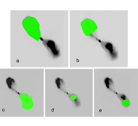
Figure 9.— Regions in the inner lobes where fluxes were measured, as given in Table 4. Measurements were done in images made by combining VTESS models with residual flux images, as discussed in Section 3.2. All images were convolved with an elliptical restoring beam 28″$\times$ 17″, oriented at position angle 11^∘.   a) The full northern inner lobe.   b The outer part of the northern inner lobe   c The full southern inner lobe;   d and   e The inner and outer parts of the southern inner lobe. (ONLINE FIGURE only)

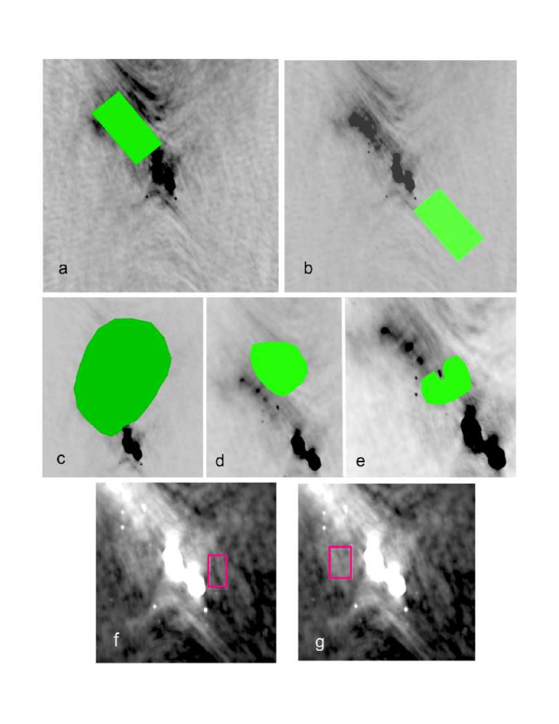
Figure 10.— Regions outside the inner lobes where fluxes were measured, as in Table 4. Images were smoothed by different size restoring beams; all restoring beams were oriented N-S.   a) The North Middle Lobe, region measured by Kraft (2009).   b) A comparable area where a South Middle Lobe might be expected. The images in both  a) and  b) have been convolved with an elliptical restoring beam 35″$\times$ 25″.   c) Full NML, in image convolved by restoring beam 70″$\times$ 60″.   d) Diffuse emission Region 3 in Table 4, shown on image with restoring beam 40″$\times$ 30″.   e) Diffuse emission Region 1 in Table 4, shown on image with restoring beam 28″$\times$ 17″.   f) and  g) Local regions #1 and #2, near but outside Inner Lobes in Table 4, both shown on images with restoring beam 35″$\times$ 25″. (ONLINE FIGURE ONLY)

References

- (1)
- (2) Bland, J., Taylor, K., Atherton, P. D., 1987, MNRAS 228, 595
- (3)
- (4) Burns, J. O., Feigelson, E. D., & Schreier, E. J. 1983, ApJ 273, 128
- (5)
- (6) Burbidge, G., 1956, ApJ 124, 416
- (7)
- (8) Burbidge, G., 1959, ApJ 129, 849
- (9)
- (10) Burns, J. O., Owen, F. N. & Rudnick, L., 1979, AJ, 84, 1683
- (11)
- (12) Clarke, D. A., Bridle, A. J., Burns, J. O., Perley, R. A. & Norman, M. L., 1992a, ApJ 385, 173.
- (13)
- (14) Clarke, D. A., Burns, J. O., & Norman, M. L., 1992b, ApJ 395, 444.
- (15)
- (16) Cornwell, T. J. & Evans, K. F., 1985, AA 143, 77
- (17)
- (18) Crockett, R. M., Shabala, S. S., Krviraj, S., et al. , 2012, MNRAS 421, 1603
- (19)
- (20) Croft, s., Van Breugel, W., de Vries, W., et al. , 2006 ApJ 647, 1040.
- (21)
- (22) Croston, J.H., Kraft, R.P., Hardcastle, M.J., et al. , 2009, MNRAS 395, 1999.
- (23)
- (24) Dufour, R. J., van den Bergh, S., Harvel, et al. , 1979, AJ 84, 284
- (25)
- (26) Eilek, J. A., 2014, New Journal of Physics 16, 045001 (E14)
- (27)
- (28) Evans, I. & Koratkar, A. 2004, ApJ 617, 209.
- (29)
- (30) Feain, I.. J., Cornwell, T.J., Ekers, R. D., et al. , 2011, ApJ 740, 17.
- (31)
- (32) Feigelsen, E. D., Schreier, E. J., Delvaille, et al. , 1981, ApJ 251, 31. 363, 91.
- (33)
- (34) Fragile, P. C., Murray, S. D., Anninos, P., & van Breugel, W., 2004, ApJ 604, 74.
- (35)
- (36) Goodger, J. L., Hardcastle, M. J., Croston, et al. , 2009, ApJ 708, 675
- (37)
- (38) Gopal-Krishna, Witta, P. J., 2010, New Astronomy 15, 96
- (39)
- (40) Graham, J. A., 1998, ApJ 502, 245
- (41)
- (42) Graham, J. A. and Price, R. M., 1981, ApJ 247, 813
- (43)
- (44) Greisen, E.W., 2003, in Information Handling in Asronomy - Historical Vistas, Astrophysics and Space Science Library, A. Heck (ed), Kluwer Academic Publishers, 109
- (45)
- (46) Hardcastle, M. J., Cheung, C. C., Feain, I. J. et al. , 2009, MNRAS 393, 1041
- (47)
- (48) Harris, G. L. H., Rejkuba, M., & Harris, W. E., 2010, PASA 27, 457.
- (49)
- (50) Haynes, R. F., Cannon, R. D., Ekers, R. D., 1983, Proc ASA 241
- (51)
- (52) Junkes, N., Haynes, R. F., Harnett, J. I.,et al. 1993, A&A269, 29.
- (53)
- (54) Kraft, R. P., Vazquez, S. E., Forman, . R., et al. , 2003, ApJ 592, 129
- (55)
- (56) Kraft, R. P., Nulsen, P. E. J., Birkinshaw, M., et al. , 2008, ApJ 665, 2007.
- (57)
- (58) Kraft, R. P., Forman, W. R., Hardcastle, M. J., et al. , 2009, ApJ 698, 2036.
- (59)
- (60) Laing, R., Guidetti, D., Bridle, A. H., Parma, P. & Bondi, M, 2011, MNRAS417 2789
- (61)
- (62) Melo, V. P., Muñoz-Tuñón, C, Maíz-Apellániz, J & Tenorio-Tagle, G., 2005, ApJ, 619, 270
- (63)
- (64) Mineo, S., Gilfanov, M., Lehmer, B. D., et al. , 2014, MNRAS 437, 1698.
- (65)
- (66) Minniti, D., Rejkuba, M., Funes, J. G., et al. , 2004, ApJ 612, 215
- (67)
- (68) Morganti, R., Killeen, N. E. B., Ekers, R. D., & Osterloo, T. A. 1999, MNRAS307, 750 (M99)
- (69)
- (70) Mould, J. R., Ridgewell, A., Gallagher, J. S., et al. , 2000, ApJ 536, 266.
- (71)
- (72) Muller, C., Kadler, M. Ojha, R., et al. , 2011, A&A 530, L11.
- (73)
- (74) Myers, S. T. & Spangler, S. R., 1985, ApJ, 291, 52
- (75)
- (76) Neff, S. G., Eilek, J. A. & Owen, F. N., 2014, to appear in ApJ (Paper 2)
- (77)
- (78) Owen, F. N., Eilek, J. A. & Kassim, N., ApJ 543, 611
- (79)
- (80) Pacholczyk, A. G., 1970, Radio Astrophysics. Nonthermal Processes in Galactic and Extragalactic Sources, p. 170.
- (81)
- (82) Quillen, A. C., Graham, J. R., and Frogel, J. A., 1993, ApJ 412, 550
- (83)
- (84) Ranalli, P., Comastri, A. & Setti, G., 2003, A&A 399, 39
- (85)
- (86) Romero, G. E., Combi, J. A., Perez Bergliaffa, S. E. & Anchordiqui, L. A., 1996, Astroparticle Physics 5, 279
- (87)
- (88) Rudnick, L. , 2002, PASP, 114, 427.
- (89)
- (90) Saxton, C. R., Sutherland, R. S., & Bicknell, G. V.. 2001, ApJ, 563, 103.
- (91)
- (92) Schreier, E. J., Burns, J. O., and Feigelson, E. D., 1981, ApJ 251, 523
- (93)
- (94) Sparke, L. S. 1996, ApJ 473, 810
- (95)
- (96) Sparks, W. B., Donahue, M., Jordan, A. et al. , 2004, ApJ 607, 294
- (97)
- (98) Stawatz, L., Aharonian, F., Wagner, S. & Ostrowski, M., 2006, MNRAS 371, 1705
- (99)
- (100) Struve, C., Oosterloo, T. A., Morganti, R. & Saripalli, L., 2010, A&A 515, A67.
- (101)
- (102) Sutherland, R. S., Bicknell, G. V. & Dopita, M. A. 1993, ApJ 414, 510.
- (103)
- (104) Tingay, S. J., Preston, R. A., and Jauncey, D. L., 2001, AJ 122, 1697
- (105)
- (106) Werner, N., Oonk, J. B. R., Canning, R. E. A., et al. , 2013, ApJ 767: 153
- (107) Whitmore, B. C., Zhang, Q., Leitherer, C., et al. , 1999, ApJ 118, 1551
- (108)
- (109) Yang, R., Sahakyan, N., Wilhelmi, E., et al. , 2012, A&A 542, 19
- (110)