On Sex, Evolution, and the Multiplicative Weights Update Algorithm

Abstract

We consider a recent innovative theory by Chastain et al. on the role of sex in evolution Chastain et al. [2014]. In short, the theory suggests that the evolutionary process of gene recombination implements the celebrated multiplicative weights updates algorithm (MWUA). They prove that the population dynamics induced by sexual reproduction can be precisely modeled by genes that use MWUA as their learning strategy in a particular coordination game. The result holds in the environments of weak selection, under the assumption that the population frequencies remain a product distribution.

We revisit the theory, eliminating both the requirement of weak selection and any assumption on the distribution of the population. Removing the assumption of product distributions is crucial, since as we show, this assumption is inconsistent with the population dynamics. We show that the marginal allele distributions induced by the population dynamics precisely match the marginals induced by a multiplicative weights update algorithm in this general setting, thereby affirming and substantially generalizing these earlier results.

We further revise the implications for convergence and utility or fitness guarantees in coordination games. In contrast to the claim of Chastain et al. [2014], we conclude that the sexual evolutionary dynamics does not entail any property of the population distribution, beyond those already implied by convergence.

“Sex is the queen of problems in evolutionary biology. Perhaps no other natural phenomenon has aroused so much interest; certainly none has sowed so much confusion.”

1 Introduction

Connections between the theory of evolution, machine learning and games have captured the imagination of researchers for decades. Evolutionary models inspired a range of applications from genetic algorithms to the design of distributed multi-agent systems Goldberg and Holland [1988]; Cetnarowicz et al. [1996]; Phelps et al. [2008]. Within game theory, several solution concepts follow evolutionary processes, and some of the most promising dynamics that lead to equilibria in games assume that players learn the behavior of their opponents Haigh [1975]; Valiant [2009].

A different connection between sex, evolution and machine learning was recently suggested by Chastain, Livnat, Papadimitriou and Vazirani [2014]. As they explain, also referring to Barton and Charlesworth [1998], sexual reproduction is costly for the individual and for the society in terms of time and energy, and often breaks successful gene combinations. From the perspective of an individual, sex dilutes his or her genes by only transferring half of them to each offspring. Thus the question that arises is why sexual reproduction is so common in nature, and why is it so successful. Chastain et al. [2014] suggest that the evolutionary process under sexual reproduction effectively implements a celebrated no-regret learning algorithm. The structure of their argument is as follows.

First, they restrict attention to a particular class of fitness landscape where weak selection holds. Informally, weak selection means that the fitness difference between genotypes is bounded by a small constant, i.e., there are no extremely good or extremely bad gene combinations. Second, they consider the distribution of each gene’s alleles as a mixed strategy in a matrix-form game, where there is one player for each gene. The game is an identical interest game, where each player gets the same utility— thus the joint distribution of alleles corresponds to the mixed strategy of each player, and the expected payoff of the game corresponds to the average fitness level of the population.

Chastain et al. [2014] provide a correspondence between the sexual population dynamics and the multiplicative weights update algorithm (MWUA) Littlestone and Warmuth [1994]; Cesa-Bianchi et al. [1997]. In particular, they establish a correspondence between strategies adopted by players in the game that adopt MWUA and the population dynamics, under an assumption that the fitness matrix is in the weak selection regime, and that the population dynamic retains the structure of a product distribution on alleles. With this correspondence in place, these authors apply the fact that using MWUA in a repeated game leads to diminishing regret for each player to conclude that the regret experienced by genes also diminishes. They interpret this result as maximization of a property of the population distribution, namely “the sum of the expected cumulative differential fitness over the alleles, plus the distribution’s entropy.”

We believe that such a multiagent abstraction of the evolutionary process can contribute much to our understanding, both of evolution and of learning algorithms. Interestingly, the agents in this model are not the creatures in the population, nor Dawkins’ Dawkins [2006] genetic properties (alleles) that compete one another, but rather genes that share a mutual cause.

1.1 Our Contribution

We show that the main results of Chastain et al. [2014] can be substantially generalized. Specifically, we consider the two standard population dynamics (where recombination acts before selection (RS), and vice versa (SR)), and show that each of them precisely describes the marginal allele distribution under a variation of the multiplicative updates algorithm that is described for correlated strategies. This correspondence holds for any number of genes/players, any fitness matrix, any recombination rate, and any initial population frequencies. In particular, and in contrast to Chastain et al., we do not assume weak selection or require the population distribution remains a product distribution (i.e., with allele probabilities that are independent), and we allow both the SR model and the RS model.

We discuss some of the implications of this correspondence between these biological and algorithmic processes for theoretical convergence properties. Under weak selection, the observation that the cumulative regret of every gene is bounded follows immediately from known convergence results, both in population dynamics and in game theory (see related work). We show that under the SR dynamics, every gene still has a bounded cumulative regret, without assuming weak selection or a product distribution.

Our analysis also uncovers what we view as one technical gap and one conceptual gap regarding the fine details in the original argument of Chastain et al. [2014]. We believe that due to the far reaching consequences of the theory it is important to rectify these details. First, according to the population dynamics the population frequencies may become highly correlated (even under weak selection), and thus it is important to avoid the assumption on product distributions. Second, the property that is supposedly maximized by the population dynamics is already entailed by the convergence of the process (regardless of what equilibrium is reached). We should therefore be careful when interpreting it as some nontrivial advantage of the evolutionary process.

1.2 Related Work

The multiplicative weights update algorithm (MWUA) is a general name for a broad class of methods in which a decision maker facing uncertainty (or a player in a repeated game), updates her strategy. While specifics vary, all variations of MWUA increase the probability of actions that have been more successful in previous rounds. In general games, the MWUA dynamic is known to lead to diminishing regret over time Jafari et al. [2001]; Blum and Mansour [2007]; Kale [2007]; Cesa-Bianchi et al. [2007], but does not, in general, converge to a Nash equilibrium of the game. For some classes of games better convergence results are known; see Section 5.2 for details.

The fundamental theorem of natural selection, which dates back to Fisher [1930], states that the population dynamics of a single-locus diploid always increases the average fitness of each generation, until it reaches convergence Mulholland and Smith [1959]; Li [1969]. The fundamental theorem further relates the rate of increase to the variance of fitness in the population. In the general case, for genotypes with more than a single locus, the fundamental theorem does not hold, although constructing a counter example where a cycle occurs is non-trivial Hastings [1981]; Hofbauer and Iooss [1984]. However, convergence of the population dynamics has been shown to hold when the fitness landscape has some specific properties, such as weak selection, or weak epistasis Nagylaki et al. [1999].

In asexual evolutionary dynamics, every descendent is an exact copy of a single parent, with more fit parents producing more offspring (“survival of the fittest”). Regardless of the number of loci, asexual dynamics coincides with MWUA by a single player Börgers and Sarin [1997]; Hopkins [1999]. Chastain et al. [2014] were the first to suggest that a similar correspondence can be established for sexual population dynamics.

2 Definitions

$w_{ij}$	$b_{1}$	$b_{2}$		$p^{0}_{ij}$	$b_{1}$	$b_{2}$	$\mathbf{y}^{0}$		$p^{1}_{ij}$	$b_{1}$	$b_{2}$	$\mathbf{y}^{0}$
$a_{1}$	1	0.5		$a_{1}$	0.1	0.15	0.25		$a_{1}$	0.094	0.082	0.174
$a_{2}$	1.5	1.2		$a_{2}$	0.1	0.15	0.25		$a_{2}$	0.158	0.170	0.328
$a_{3}$	1.3	0.8		$a_{3}$	0.2	0.3	0.5		$a_{3}$	0.255	0.242	0.497
				$\mathbf{x}^{0}$	0.4	0.6			$\mathbf{x}^{1}$	0.507	0.493

Table 1: An example of a 2-locus haploid fitness matrix, with $n=3,m=2$. There are 6 allele combinations, or genotypes. On the left we give the fitness of each combination $\left\langle a_{i},b_{j}\right\rangle$. In the middle, we provide an initial population distribution, and on the right we provide the distribution after one update step of the SR dynamics, for $r=0.5$.

We follow the definitions of Chastain et al. [2014] where possible. For more detailed explanation of the biological terms and equations, see Bürger [2011].

2.1 Population dynamics

A haploid is a creature that has only one copy of each gene. Each gene has several distinct alleles. For example, a gene for eye color can have alleles for black, brown, green or blue color. In contrast, people are diploids, and have two copies of each gene, one from each parent.

Under asexual reproduction, an offspring inherits all of its genes from its single parent. In the case of sexual reproduction, each parent transfers half of its genes. Thus a haploid inherits half of its properties from one parent and half from the other parent. To keep the presentation simple we focus on the case of a 2-locus haploid. This means that there are two genes, denoted $A$ and $B$. In the appendix we extend the definitions and results to $k$-locus haploids, for $k>2$. Gene $A$ has $n$ possible alleles $a_{1},\ldots,a_{n}$, and gene $B$ has $m$ possible alleles $b_{1},\ldots,b_{m}$. It is possible that $n\neq m$. We denote the set $\{1,\ldots,n\}$ by $[n]$. A pair $\left\langle a_{i},b_{j}\right\rangle$ of alleles defines a genotype.

Let $W=(w_{ij})_{i\leq n,j\leq m}$ denote a fitness matrix. The fitness value $w_{ij}\in\mathbb{R}_{+}$ can be interpreted as the expected number of offspring of a creature whose genotype is $\left\langle a_{i},b_{j}\right\rangle$. We assume that the fitness matrix is fixed, and does not change throughout evolution. See Table 1 for an example.

We denote by $P^{t}=(p_{ij}^{t})_{i\leq n,j\leq m}$ the distribution of the population at time $t$. The average fitness $\overline{w}^{t}$ at time $t$ is written as

$$\overline{w}^{t}=\overline{w}(P^{t})=\sum_{ij}p^{t}_{ij}w_{ij}.$$ (1)

For example, the populations in Table 1 have an average fitness of $\overline{w}(P^{0})=1.005$ and $\overline{w}(P^{1})=1.1012$. Denote by $x^{t}_{i}=\sum_{j}p^{t}_{ij}$ and $y^{t}_{j}=\sum_{i}p^{t}_{ij}$ the marginal frequencies at time $t$ of alleles $a_{i}$ and $b_{j}$, respectively. Clearly $p^{t}_{ij}=x^{t}_{i}y^{t}_{j}$ for all $i,j$ iff $P^{t}$ is a product distribution. In the context of population dynamics, the set of product distributions is also called the Wright manifold. For general distributions, $D^{t}_{ij}=p^{t}_{ij}-x^{t}_{i}y^{t}_{j}$ is called the linkage disequilibrium.

The selection strength of $W$ is the minimal $s$ s.t. $w_{ij}\in[1-s,1+s]$ for all $i,j$. We say that $W$ is in the weak selection regime if $s$ is very small, i.e., all of $w_{ij}$ are close to $1$.

Update step

In asexual reproduction, every creature of genotype $\left\langle a_{i},b_{j}\right\rangle$ has in expectation $w_{ij}$ offspring, all of which are of genotype $\left\langle a_{i},b_{j}\right\rangle$. Thus there is only selection and no recombination, and the frequencies in the next period are $p^{t+1}_{ij}=p^{S}_{ij}=\frac{w_{ij}}{\overline{w}^{t}}p^{t}_{ij}$.

In sexual reproduction, every pair of creatures, say of genotypes $\left\langle a_{i},b_{l}\right\rangle$ and $\left\langle a_{k},b_{j}\right\rangle$ bring offspring who may belong (with equal probabilities) to genotype $\left\langle a_{i},b_{l}\right\rangle,\left\langle a_{k},b_{j}\right\rangle,\left\langle a_{i},b_{j}\right\rangle$, or $\left\langle a_{k},b_{l}\right\rangle$. Thus, in the next generation, a creature of genotype $\left\langle a_{i},b_{j}\right\rangle$ can be the result of combining one parent of genotype $\left\langle a_{i},?\right\rangle$ with another parent of genotype $\left\langle?,b_{j}\right\rangle$. There are two ways to infer the distribution of the next generation, depending on whether recombination occurs before selection or vice versa (see, e.g., Michalakis and Slatkin [1996]). We describe each of these two ways next.

Selection before recombination (SR)

Summing over all possible matches and their frequencies, and normalizing, we get:

$$p^{SR}_{ij}=\frac{\sum_{l\in[m]}\sum_{k\in[n]}p^{t}_{il}w_{il}p^{t}_{kj}w_{kj}}{(\overline{w}^{t})^{2}}.$$

In addition, the recombination rate, $r\in[0,1]$, determines the part of the genome that is being replaced in crossover, so $r=1$ means that the entire genome is the result of recombination, whereas $r=0$ means no recombination occurs, and the offspring are genetically identical to one of their parents. Given this, population frequencies in the next period are set as:

$$p^{t+1}_{ij}=rp^{SR}_{ij}+(1-r)p^{S}_{ij}.$$ (2)

Recombination before selection (RS)

With only recombination, the frequency of the genotype $\left\langle a_{i},b_{j}\right\rangle$ is the product of the respective probabilities in the previous generation, i.e., $p^{R}_{ij}=x^{t}_{i}y^{t}_{j}$. When recombination occurs before selection, we have (before normalization):

$$p^{RS}_{ij}=w_{ij}p^{R}_{ij}=w_{ij}x^{t}_{i}y^{t}_{j}.$$

Taking into account the recombination rate and normalization, we get,

$$p^{t+1}_{ij}=\frac{1}{\overline{w}^{R}}(rp^{RS}_{ij}+(1-r)p^{S}_{ij})=\frac{1}{\overline{w}^{R}}w_{ij}(p^{t}_{ij}-rD^{t}_{ij}),$$ (3)

where $\overline{w}^{R}=\sum_{ij}w_{ij}(p^{t}_{ij}-rD^{t}_{ij})$, and $D^{t}_{ij}$ is the linkage disequilibrium at time $t$.

For an example of change in population frequencies, see Tables 1-4. We say that $P^{t}$ is a stable state under a particular dynamics, if $P^{t+1}=P^{t}$.

2.2 Identical interest games

An identical interest game of two players is defined by a payoff matrix $G$, where $g_{ij}$ is the payoff of each player if the first plays action $i$, and the second plays action $j$. A mixed strategy of a player is an independent distribution over her actions. The mixed strategies $\mathbf{x},\mathbf{y}$ are a Nash equilibrium if no player can switch to a strategy that has a strictly higher expected payoff. That is, if for any action $i^{\prime}\in[n]$, $\sum_{j}y_{j}g_{i^{\prime}j}\leq\sum_{i}\sum_{j}x_{i}y_{i}g_{ij}$, and similarly for any $j^{\prime}\in[m]$.

Every fitness matrix $W$ induces an identical interest game, where $g_{ij}=w_{ij}$. This is a game where each of the two genes selects an allele as an action (or a distribution over alleles, as a mixed strategy). A matrix of population frequencies $P$ can be thought of as correlated strategies for the players. The expected payoff of each player under these strategies is $\overline{w}(P)$. Given a distribution $P$, $G|_{P}$ is the subgame of $G$ induced by the support of $P$. That is, the subgame where action $i$ is allowed iff $p_{ij}>0$ for some $j$, and likewise for action $j$.

2.3 Multiplicative updates algorithms

Suppose that two players play a game $G$ (not necessarily identical interest) repeatedly. Each player observes the strategy of her opponent in each turn, and can change her own strategy accordingly.One prominent approach is to gradually put more weight (i.e., probability) on pure actions that were good in the previous steps. Many variations of the multiplicative weights update algorithm (MWUA) are built upon this idea, and some have been applied to strategic settings Blum and Mansour [2007]; Marden et al. [2009]; Kleinberg et al. [2009]. We follow the variation used by Chastain et al. [2014]. This variation is equivalent to the Polynomial Weights (PW) algorithm [2007], under the assumption that the utility of all actions $(a_{i})_{i\leq n}$ is observed after each period (see Kale [2007], p. 10).

$p^{1}_{ij}$ (SR)	$b_{1}$	$b_{2}$	$\mathbf{y}^{1}$		$p^{1}_{ij}$ (RS)	$b_{1}$	$b_{2}$	$\mathbf{y}^{1}$
$a_{1}$	0.088	0.085	0.174		$a_{1}$	0.099	0.074	0.174
$a_{2}$	0.167	0.162	0.328		$a_{2}$	0.149	0.179	0.328
$a_{3}$	0.252	0.245	0.497		$a_{3}$	0.258	0.239	0.497
$\mathbf{x}^{1}$	0.507	0.493			$\mathbf{x}^{1}$	0.507	0.493

Table 2: Population frequencies $P^{1}$, i.e. after one update step, for $r=1$. On the left, we provide frequencies when selection occurs before recombination, whereas on the right recombination precedes selection. The updated marginal frequencies of alleles are the same in both cases.

$p^{1}_{ij}$ (SR)	$b_{1}$	$b_{2}$	$\mathbf{y}^{1}$		$p^{1}_{ij}$ (RS)	$b_{1}$	$b_{2}$	$\mathbf{y}^{1}$
$a_{1}$	0.094	0.082	0.174		$a_{1}$	0.099	0.074	0.174
$a_{2}$	0.158	0.170	0.328		$a_{2}$	0.149	0.179	0.328
$a_{3}$	0.255	0.242	0.497		$a_{3}$	0.258	0.239	0.497
$\mathbf{x}^{1}$	0.507	0.493			$\mathbf{x}^{1}$	0.507	0.493

Table 3: Population frequencies $P^{1}$ for $r=0.5$. Under RS we get the same frequencies as with $r=1$ (and in fact any other value of $r$). This is because when $P^{0}$ is a product distribution there is no effect of recombination under RS.

$p^{2}_{ij}$ (SR)	$b_{1}$	$b_{2}$	$\mathbf{y}^{2}$		$p^{2}_{ij}$ (RS)	$b_{1}$	$b_{2}$	$\mathbf{y}^{2}$
$a_{1}$	0.079	0.042	0.122		$a_{1}$	0.09	0.034	0.124
$a_{2}$	0.228	0.172	0.401		$a_{2}$	0.203	0.195	0.398
$a_{3}$	0.294	0.183	0.477		$a_{3}$	0.305	0.173	0.478
$\mathbf{x}^{2}$	0.602	0.398			$\mathbf{x}^{2}$	0.598	0.402

Table 4: Population frequencies $P^{2}$, i.e. after two update steps for $r=0.5$. The marginal distributions are no longer the same, since $P^{1}$ under RS is not a product distribution.

Polynomial Weights

We use the term PW to distinguish this from other variations of MWUA. For any $\epsilon>0$, the $\epsilon$-PW algorithm for a single decision maker is defined as follows. Suppose first that in time $t$, the player uses strategy $\mathbf{x}^{t}$. Let $g^{t}_{i}$ be the utility to the player when playing some pure action $i\in[n]$. According to the $\epsilon$-PW algorithm, the strategy of the player in the next step would be $x^{t+1}(i)\cong x^{t}(i)(1+\epsilon g^{t}_{i})$, where $\cong$ stands for “proportional to” (we need to normalize, since $\mathbf{x}^{t+1}$ has to be a valid distribution). A special case of the algorithm is the limit case $\epsilon\rightarrow\infty$, where $x^{t+1}(i)\cong x^{t}(i)g^{t}_{i}$; i.e., the probability of playing an action increases proportionally to its expected performance in the previous round. Unless specified otherwise we assume this limit case, which we refer to as the parameter-free PW.

PW in Games

The fundamental feature of the PW algorithm is that the probability of playing action $a_{i}$ changes proportionally to the expected utility of action $a_{i}$.

Consider 2-player game $G$, where $g_{ij}$ is the utility (of both players if $G$ is an identical interest game) from the joint action $\left\langle a_{i},b_{j}\right\rangle$. In the context of a game, we can think of at least two different interpretations of the utility of playing $a_{i}$, derived from the joint distribution $P$. For this, let $y^{t}_{j}(a_{i})=P^{t}(b_{j}|a_{i})$, i.e., the probability that player 2 plays $b_{j}$ given that player 1 plays $a_{i}$, according to the distribution $P^{t}$. The two interpretations we have in mind are:

• Set $\underline{g}^{t}_{i}=\sum_{j}y^{t}_{j}(a_{i})g_{ij}$. This is the expected utility that player 1 would get for playing $a_{i}$ in round $t$. This definition is consistent with common interpretation of expected utility in games (e.g., in Kale [2007], Sec. 2.3.1).

• Set $\overline{g}^{t}_{i}=\sum_{j}y^{t}_{j}g_{ij}$. This is the expected utility that player 1 will get in the next round for playing $a_{i}$ if player 2 will select an action independently according to her current marginal probabilities. Thus each agent updates her strategy as if the strategies are independent, and ignoring any observed correlation. This definition results in the PW algorithm used in Chastain et al. [2014].

The above definitions require some discussion. While the traditional assumption is that each player only observes a sample from the joint distribution at each round, and updates the strategy based on the empirical distribution, strategy updates can also be performed in the same way when the player observes the joint distribution at round $t$, even if it is hard to imagine such a case occurs in practice.

Intuitively, under the first interpretation, the player considers correlation, whereas under the second the player assumes independence, and then uses the marginals to compute the expected utility. E.g suppose that players play Rock-Paper-Scissors, and the history is 100 repetitions of the sequence [(R,P) (P,S) (S,S)]. Then under the first interpretation the best action for agent 1 is S (since it leads to the best expected utility); whereas under the second interpretation the best action for agent 1 is R, since agent 2 is more likely to play S. Clearly, when $P^{t}$ is a product distribution (as in Chastain et al. [2014]) then $\overline{g}^{t}_{i}=\underline{g}^{t}_{i}$, and the algorithms coincide. We can also combine the two interpretations to induce new algorithms. We thus define the PW^(α) algorithm (either Parameter-free PW^(α) or $\epsilon$-PW^(α)), where the probability of playing $a_{i}$ is updated according to $g^{t,(\alpha)}_{i}=\alpha\overline{g}^{t}_{i}+(1-\alpha)\underline{g}^{t}_{i}$.

Exponential Weights

The Hedge algorithm Freund and Schapire [1995, 1999] is another variation of MWUA that is very similar to PW. The difference is that the weight of action $i$ in each step changes by a factor that is exponential in the utility, rather than linear. That is, $x^{t+1}(i)\cong x^{t}(i)(1+\epsilon)^{g^{t}_{i}}$. For negligible $\epsilon>0$, $\epsilon$-Hedge and $\epsilon$-PW are essentially the same, but for large $\epsilon$ they may behave quite differently.

3 Analysis of the SR dynamics

In this section we prove that the SR population dynamics of marginal allele frequencies coincide precisely with the multiplicative updates dynamics in the corresponding game. This extends Theorem 4 in Chastain et al. [2014] (SI text), in that it holds without weak selection or the assumption of product distributions through multiple iterations. We also generalize the proposition to hold for any number of loci/players in Appendix A.

Proposition 1.

Let $W$ be any fitness matrix, and consider the game $G$ where $g_{ij}=w_{ij}$. Then under the SR population dynamics, for any distribution $P^{t}$ and any $r\in[0,1]$, we have $x^{t+1}_{i}=\frac{1}{\overline{w}^{t}}x^{t}_{i}\underline{g}^{t}_{i}$.

Proof.

By the SR population dynamics (Eq. (2)),

$$x^{t+1}_{i} =\sum_{j}p^{t+1}_{ij}=\sum_{j}(rp^{SR}_{ij}+(1-r)p^{S}_{ij})$$

$$=r\sum_{j}\frac{\sum_{l}\sum_{k}p^{t}_{il}w_{il}p^{t}_{kj}w_{kj}}{(\overline{w}^{t})^{2}}+(1-r)\sum_{j}\frac{p^{t}_{ij}w_{ij}}{\overline{w}^{t}}$$

$$=r\frac{1}{\overline{w}^{t}}\sum_{l}p^{t}_{il}w_{il}\frac{1}{\overline{w}^{t}}\sum_{k}\sum_{j}p^{t}_{kj}w_{kj}+(1-r)\sum_{j}\frac{p^{t}_{ij}w_{ij}}{\overline{w}^{t}}$$

Then since $\sum_{k}\sum_{j}p^{t}_{kj}w_{kj}$ is the average fitness at time $t$,

$$x^{t+1}_{i} =r\frac{1}{\overline{w}^{t}}\sum_{j}p^{t}_{ij}w_{ij}\frac{1}{\overline{w}^{t}}\overline{w}^{t}+(1-r)\sum_{j}\frac{p^{t}_{ij}w_{ij}}{\overline{w}^{t}}$$

$$=r\frac{1}{\overline{w}^{t}}\sum_{j}p^{t}_{ij}w_{ij}+(1-r)\sum_{j}\frac{p^{t}_{ij}w_{ij}}{\overline{w}^{t}}$$

$$=\frac{1}{\overline{w}^{t}}\sum_{j}p^{t}_{ij}w_{ij}=\frac{1}{\overline{w}^{t}}\sum_{j}x^{t}_{i}y^{t}_{j}(a_{i})w_{ij},$$

thus the recombination factor $r$ does not play a direct role in the new marginal under the SR dynamics. It does have an indirect role though, since it affects the correlation, and thus the marginal distribution at the next generation $t+2$. ∎

Theorem 4 in Chastain et al. [2014] follows as a special case when $P^{t}$ is a product distribution. By repeatedly applying Proposition 1, we get the following result, which holds for any value of $r$.

Corollary 1.

Let $W$ be a fitness matrix, $P^{0}$ be any distribution. Suppose that $P^{t+1}$ is attained from $P^{t}$ by the SR population dynamics, and that $\mathbf{x}^{t+1},\mathbf{y}^{t+1}$ are attained from $P^{t}$ by players using the parameter-free PW⁽⁰⁾ algorithm in the game $G=W$. Then for all $t>0$ and any $i$, $x^{t}_{i}=\sum_{j}p^{t}_{ij}$.

It is important to note that the marginal distributions $\mathbf{x}^{t},\mathbf{y}^{t}$ do not determine $P^{t}$ completely. Thus the PW algorithm specifies the strategy of each player (regardless of $r$), but not how these strategies are correlated.

4 Analysis of the RS dynamics

Turning to the RS population dynamics, our starting point is Lemma 3 in Chastain et al. [2014] (SI text), which states that $p^{t+1}_{ij}=\frac{1}{\overline{w}^{R}}w_{ij}x^{t}_{i}y^{t}_{j}$ (under the assumption that $P^{t}$ is a product distribution). We establish a similar property for general distributions. We use the fact that for any fitness matrix $W$ and distribution $P^{t}$,

$$p^{t+1}_{ij}=\frac{1}{\overline{w}^{R}}(rw_{ij}x^{t}_{i}y^{t}_{j}+(1-r)w_{ij}p^{t}_{ij}).$$

This follows immediately from the definition (Eq. (3)). Recall that $g^{t,(r)}_{i}=\left(r\overline{g}^{t}_{i}+(1-r)\underline{g}^{t}_{i}\right)$. We derive an alternative extension of Theorem 4 in Chastain et al. [2014] (SI text) for the RS dynamics.

Proposition 2.

Let $W$ be any fitness matrix, and consider the game $G$ where $g_{ij}=w_{ij}$. Then under the RS population dynamics, for any distribution $P^{t}$ and any $r\in[0,1]$, $x^{t+1}_{i}=\frac{1}{\overline{w}^{R}}x^{t}_{i}g^{t,(r)}_{i}$.

Proof.

By the RS population dynamics (Eq. (3)),

$$x^{t+1}_{i} =\sum_{j}p^{t+1}_{ij}=\sum_{j}\frac{1}{\overline{w}^{R}}(rw_{ij}x^{t}_{i}y^{t}_{j}+(1-r)w_{ij}p^{t}_{ij})$$

$$=\frac{1}{\overline{w}^{R}}\sum_{j}(rw_{ij}x^{t}_{i}y^{t}_{j}+(1-r)w_{ij}x^{t}_{i}y^{t}_{j}(a_{i}))$$

$$=\frac{1}{\overline{w}^{R}}x^{t}_{i}(r\sum_{j}w_{ij}y^{t}_{j}+(1-r)\sum_{j}w_{ij}y^{t}_{j}(a_{i})).$$

Finally, by the definitions of $\overline{g}^{t}_{i}$ and $\underline{g}^{t}_{i}$,

$$x^{t+1}_{i}=\frac{1}{\overline{w}^{R}}x^{t}_{i}\left(r\overline{g}^{t}_{i}+(1-r)\underline{g}^{t}_{i}\right)=\frac{1}{\overline{w}^{R}}x^{t}_{i}g^{t,(r)}_{i}.$$

In contrast to the SR dynamics, here $r$ appears explicitly in the marginal distribution $\mathbf{x}^{t+1}$. ∎

So we get that under RS the marginal frequency of allele $a_{i}$ is updated according to an expected utility that takes only part of the correlation into account. This part is proportional to the recombination rate $r$. We get a similar result to Corollary 1:

Corollary 2.

Let $W$ be a fitness matrix, $P^{0}$ be any distribution. Suppose that $P^{t+1}$ is attained from $P^{t}$ by the RS population dynamics, and that $\mathbf{x}^{t+1},\mathbf{y}^{t+1}$ are attained from $P^{t}$ by players using the parameter-free PW^(r) algorithm in the game $G=W$. Then for all $t>0$ and any $i$, $x^{t}_{i}=\sum_{j}p^{t}_{ij}$.

5 Convergence and Equilibrium

In this section, we consider implications of the general theory on the correspondence between sexual population dynamics and multiplicative-weights algorithms on convergence properties.

5.1 Diminishing regret

In Chastain et al. [2014] (Sections 3 and 4 of the SI text), the authors apply standard properties of MWUA to show that the cumulative external regret of each gene is bounded (Corollary 5 there). In other words, if in retrospect gene 1 would have “played” some fixed allele $a_{i}$ throughout the game, the cumulative fitness (summing over all iterations) would not have been much better. This result leans only on the properties of the algorithm, and does not require the independence of strategies. Thus we will write a similar regret bound explicitly in our more general model.

Consider any fitness matrix $W$ whose selection strength is $s$. Let $AF^{T}_{i}=\frac{1}{T}\sum_{t=1}^{T}\underline{g}^{t}_{i}$ (the average fitness in retrospect if allele $a_{i}$ had been used throughout the game), and $AF_{SR}^{T}=\frac{1}{T}\sum_{t=1}^{T}\overline{w}^{t}$ (the actual average fitness under the SR dynamics).

Corollary 3.

For any $T\in\mathbb{N}$, any $s\in(0,\frac{1}{2})$ and all $i\leq n$, $AF_{SR}^{T}\geq AF^{T}_{i}-s^{2}-\ln(n)/T$.

Proof.

Set $\Delta_{ij}=\frac{w_{ij}-1}{s}$; $m^{(t)}_{i}=\sum_{j}y^{t}_{j}(a_{i})\Delta_{ij}$, and $\epsilon=s$. Note that $\Delta_{ij}$ and $m^{(t)}_{i}$ are in the range $[-1,1]$. Intuitively, $m^{(t)}_{i}$ is the expected profit of player 1 from playing action $a_{i}$ in the “differential game” $\frac{W-1}{s}$.

Theorem 3 Kale [2007] states that under the $\epsilon$-PW algorithm

$$\sum_{t=1}^{T}\mathbf{x}^{(t)}\mathbf{m}^{(t)}\geq\sum_{t=1}^{T}m_{i}^{(t)}-\epsilon\sum_{t=1}^{T}(m_{i}^{(t)})^{2}-\frac{\ln(n)}{\epsilon},$$ (4)

where $x^{(t)}_{i}$ is the probability that the decision maker chose action $a_{i}$ in iteration $t$ (thus $x^{(t)}_{i}=x^{t}_{i}$ by our notation).

The proof follows directly from the theorem. Observe that $m^{(t)}_{i}=(\underline{g}^{t}_{i}-1)/s$, and

$$\mathbf{x}^{(t)}\cdot\mathbf{m}^{(t)} =\sum_{i}x^{t}_{i}m^{(t)}_{i}=\sum_{i}x^{t}_{i}\sum_{j}y^{t}_{j}(a_{i})\Delta_{ij}$$

$$=\sum_{ij}p^{t}_{ij}\frac{w_{ij}-1}{s}=\frac{\overline{w}^{t}-1}{s}.$$

Thus

$$AF_{i}^{T} =\frac{1}{T}\sum_{t=1}^{T}\underline{g}^{t}_{i}=\frac{1}{T}\sum_{t=1}^{T}sm^{(t)}_{i}+1=1+\epsilon\frac{1}{T}\sum_{t=1}^{T}m^{(t)}_{i}$$

$$AF_{SR}^{T} =\frac{1}{T}\sum_{t=1}^{T}\overline{w}^{t}=\frac{1}{T}\sum_{t=1}^{T}(1+s\mathbf{m}^{(t)}\cdot\mathbf{p}^{(t)})$$

$$=1+\epsilon\frac{1}{T}\sum_{t=1}^{T}\mathbf{m}^{(t)}\cdot\mathbf{p}^{(t)}. \epsilon=s$$ (replacing )

Plugging in Eq. (4),

$$AF_{SR}^{T} \geq 1+\epsilon\frac{1}{T}\left(\sum_{t=1}^{T}m_{i}^{(t)}-\epsilon\sum_{t=1}^{T}(m_{i}^{(t)})^{2}-\frac{\ln(n)}{\epsilon}\right)$$

$$\geq 1+\epsilon\frac{1}{T}\left(\sum_{t=1}^{T}m_{i}^{(t)}-\epsilon\sum_{t=1}^{T}1-\frac{\ln(n)}{\epsilon}\right)$$

$$=\left(1+\epsilon\frac{1}{T}\sum_{t=1}^{T}m_{i}^{(t)}\right)-\epsilon^{2}-\frac{1}{T}\ln(n)$$

$$=AF_{i}^{T}-s^{2}-\ln(n)/T,$$

as required. ∎

We highlight that the bound on the regret of each player (or gene) stated in this result depends only on the algorithm used by the agent, and not on the strategies of other agents. These may be independent, correlated, or even chosen in an adversarial manner. For simplicity we present the proof for two players/genes. The extension to any number of players is immediate because the theorem bounds the regret of each agent separately.

By taking $s$ to zero and $T$ to infinity, we get that the average cumulative regret $AF_{SR}^{T}-AF^{T}_{i}$ tends to zero, as stated in Chastain et al. [2014] (they use a more refined form of the inequality that contains the entropy of $P^{t}$ rather than $\ln n$).

For the RS dynamics we get something similar but not quite the same. Since $g^{t,(r)}_{i}$ is not exactly the expected fitness at time $t$, we get that cumulative regret is diminishing but not w.r.t. the actual average fitness $\overline{w}^{t}$. That is, the regret is determined as if the actual expected fitness of action $a_{i}$ is $g^{t,(r)}_{i}$. More formally, we get a variation of Corollary 3, where $AF^{T}_{i}=\frac{1}{T}\sum_{t=1}^{T}g^{t,(r)}_{i}$ and $AF_{RS}^{T}=\frac{1}{T}\sum_{t=1}^{T}\sum_{i}x^{t}_{i}g^{t,(r)}_{i}$.

5.2 Convergence under weak selection

In normal-form games, following strategies with bounded or diminishing regret does not, in general, guarantee convergence to a fixed point in the strategy space. For some classes of games though, much more is known. For example, if all players in a potential game apply the $\epsilon$-Hedge algorithm, with a sufficiently small $\epsilon$, then $P^{t}$ converges to a Nash equilibrium Kleinberg et al. [2009], and almost always to a pure Nash equilibrium. Similar results have been shown for concave games Even-Dar et al. [2009]. Since identical-interest games are both potential games and concave games, and since for small $\epsilon$ we have that Hedge and PW are essentially the same, these results apply to our setting. This means that under each of RS and SR dynamics, the population converges to a stable state, for a sufficiently low selection strength $s$.

This implication is not new, and has been shown independently in the evolutionary biology literature. Indeed, Nagylaki et al. [1999] prove that under weak selection, the population dynamics converges to a point distribution from any initial state (that is, to a Nash equilibrium of the subgame induced by the support of the initial distribution). Note that under weak selection, Corollary 3 becomes trivial: once in a pure Nash equilibrium $(a_{i^{*}},b_{j^{*}})$ (say at time $t^{*}$), the optimal action of agent 1 is to keep playing $a^{*}_{i}$. Thus for any $t>t^{*}$, $\overline{w}^{t}=\underline{g}^{t}_{i^{*}}$, and the cumulative regret does not increase further.

6 Discussion

Chastain et al. [2014] extend an interesting connection between evolution, learning, and games from asexual reproduction (i.e., replicator dynamics) to sexual reproduction. The proof of Theorem 4 in Chastain et al. [2014] gives a formal meaning to this connection. Namely, that the strategy update of each player who is using PW⁽¹⁾ in the fitness game, coincides with the change in allele frequencies of the corresponding gene (under weak selection and product distributions). This relation is generalized in our Propositions 1 and 2, since for product distributions PW^(α) is the same for all $\alpha$.

Chastain et al. [2014] also claim something stronger: that the population dynamics is precisely the PW dynamics. The natural formal interpretation of this conclusion would be in the spirit of our Corollary 1, i.e., that allele distributions and players’ strategies would coincide after any number of steps. In our case we prove this for the marginal probabilities. But as we have discussed, their conclusion only follows from their Theorem 4 under the assumption that $P^{t}$ remains a product distribution. This is counterfactual, in that $P^{t+1}$ is in general not a product distribution (under their assumptions on the dynamic process), and thus the next step of the PW^(r) algorithm and the population dynamics would not be precisely equivalent but only approximately equivalent. The approximation becomes less accurate in each step, and in fact even under weak selection the population dynamics may diverge from the Wright manifold, or converge to a different outcome than the PW^(r) algorithm, as we show in Appendix B. Thus while the intuition of Chatain et al. [2014] was correct, the only way to rectify their analysis is via the more general proof without assumptions on the selection strength (even if we accept weak selection as biologically plausible).

What does evolution maximize?

In Chastain et al. [2014] (Corollary 5 in the SI text), it is also shown that under weak selection, “population genetics is tantamount to each gene optimizing at generation $t$ a quantity equal to the cumulative expected fitness over all generations up to $t$,” (plus the entropy). While this is technically correct (our Cor. 3 is a restatement of this result), we feel that an unwary reader might reach the wrong impression, that this is a mathematical explanation of some guarantee on the average fitness of the population. We thus emphasize that the both [2014] and our paper establish only the property of diminishing regret, which is already implied when $P^{t}$ converges to a Nash equilibrium. Players never have regret in a Nash equilibrium, and thus the cumulative regret tends to zero after the equilibrium is played sufficiently many times.

Thus the population dynamics cannot provide any guarantees on fitness (or on any other property) that are not already implied by an arbitrary Nash equilibrium. In the evolutionary context this means that the outcome can be as bad as the worst local maximum of the fitness matrix. Also note that convergence is to a point distribution (a pure Nash equilibrium, see Sec. 5.2), and thus its entropy is $0$ and irrelevant for the maximization claim.

Convergence without weak selection

It is an open question as to what other natural conditions are sufficient to guarantee convergence of sexual population dynamics. We have conducted simulations that show that convergence to a pure equilibrium occurs w.h.p. even without weak selection, and in fact the convergence speed increases as selection strength $s$ (or the learning rate $\epsilon$) grows. At the same time, the quality of the solution/population reached seems to be the same regardless of the selection strength/learning rate (we measured quality as the fitness of the local maximum the dynamics converged to, normalized w.r.t. the global maximum). Both trends are visible in Figure 1 for $8\times 5$ matrices, based on 1000 instances for each plot. Similar results are obtained with other sizes of matrices.

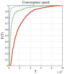
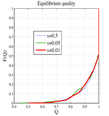
Figure 1: On the left, $F(T)$ is the fraction of instances that converge (reach $\max_{ij}p^{t}_{ij}>1-10^{-5}$) within at most $T$ generations. On the right, $F(Q)$ is the fraction of instances that converge to an equilibrium with quality $q$ at most $Q$, where $q=\frac{\overline{w}^{t}-1}{\max_{ij}w_{ij}-1}$ (the ratio between average fitness in the equilibrium that was reached, and the optimal fitness). Results are for random fitness matrices of size $8\times 5$, where $w_{ij}$ is sampled uniformly at random from $[1-s,1+s]$. Note that most instances do not converge to the optimal outcome.

However, it is known that the sexual population dynamics on general fitness matrices (even on $4\times 4$ matrices) does not always converge, and explicit examples have been constructed Hastings [1981]; Akin [1983]; Hofbauer and Iooss [1984]. By Corollaries 1 and 2, convergence of the PW algorithm to a pure Nash equilibrium, and convergence of the population dynamics to a point distribution is the same thing. Thus characterizing the conditions under which these dynamics converge will answer two questions at once.

Conclusions

We formally describe a precise connection between population dynamics and the multiplicative weights update algorithm. For this connection, we adopt a version of MWUA that takes the correlation of player strategies into account, while still supporting no regret claims. More specifically, two different variations of the Polynomial Weights subclass of MWUA each coincide with the marginal allele distribution under the two common sexual population dynamics (SR and RS). It is important to note that the correspondence that we establish is between the marginal frequencies/probabilities, rather than the full joint distribution.

Notably, weak selection is not required to make these connections.Yet, it is known that weak selection provides an additional guarantee, which is that the dynamics converge to a particular population distribution Nagylaki [1993]. It remains an open question to understand what other conditions are sufficient for convergence of the PW algorithm in identical interest games. Solving this question will also uncover more cases where the fundamental theorem of natural selection applies.

Appendix A Extension to Multiple Genes

A $k$-locus haploid has $k$ genes, each of which is inherited from one of its two parents. In this appendix we show how to extend our main results to a haploid with $k>2$ loci.

A.1 Notation

We consider a haploid with $k$ loci, each with $n_{j}$ alleles, $j\leq k$. We denote $K=[k]=\{1,2,\ldots,k\}$, and use $J$ to denote subsets of $K$.

A genotype is defined by a vector of indices $\mathbf{i}_{K}=\left\langle i_{1},\ldots,i_{k}\right\rangle$ for $i_{j}\in[n_{j}]$. We denote by ${\cal I}(J)$ the set of all $\prod_{j\in J}n_{j}$ partial index vectors of the form $\left\langle i_{j}\right\rangle_{j\in J}$. We sometimes concatenate two or more partial genotypes: $\mathbf{i}^{\prime\prime}_{J^{\prime\prime}}=\left\langle\mathbf{i}_{J},\mathbf{i}^{\prime}_{J^{\prime}}\right\rangle$ for some $\mathbf{i}_{J}\in{\cal I}(J),\mathbf{i}^{\prime}_{J^{\prime}}\in{\cal I}(J^{\prime})$. We use $-J$ to denote $K\setminus J$.

The fitness of a genotype $\mathbf{i}_{K}$ is denoted by $w_{\mathbf{i}_{K}}$. $W=(w_{\mathbf{i}_{K}})_{\mathbf{i}_{K}\in{\cal I}(K)}$ is called the fitness landscape (which is a matrix for $k=2$). Similarly, the population frequency of genotype $\mathbf{i}_{K}$ at time $t$ is denoted by $p_{\mathbf{i}_{K}}^{t}$, and $P^{t}=(p^{t}_{\mathbf{i}_{K}})_{\mathbf{i}_{K}\in{\cal I}(K)}$.

The average fitness at time $t$ is

$$\overline{w}^{t}=\sum_{\mathbf{i}_{K}\in{\cal I}(K)}p^{t}_{\mathbf{i}_{K}}w_{\mathbf{i}_{K}}=\sum_{i_{1}=1}^{n_{1}}\cdots\sum_{i_{k}=1}^{n_{k}}p^{t}_{\mathbf{i}_{K}}w_{\mathbf{i}_{K}}.$$ (5)

Let $\mathbf{x}^{t}_{j}$ be the marginal distribution of locus $j\in K$ at time $t$, i.e., for all $i_{j}\in[n_{j}]$,

$$x^{t}_{i_{j}}=\sum_{\mathbf{i}_{-j}\in{\cal I}(-j)}p^{t}_{i_{j},\mathbf{i}_{-j}}.$$

In the special case of 2 loci, $K=\{1,2\}$, and $x^{t}_{i_{1}},x^{t}_{l_{2}}$ correspond to $x^{t}_{i},y^{t}_{l}$ as used in the main text. We also define the marginal fitness of allele $i_{j}\in[n_{j}]$ at time $t$ as the average fitness of all the population with allele $i_{j}$. That is,

$$w^{t}_{i_{j}}=\sum_{\mathbf{i}_{-j}\in{\cal I}(-j)}p^{t}(\mathbf{i}_{-j}|i_{j})w_{i_{j},\mathbf{i}_{-j}}.$$ (6)

A.2 RS dynamics

According to the multi-dimensional extension of $p^{t+1}_{\mathbf{i}_{K}}$,

$$p^{t+1}_{\mathbf{i}_{K}}=\frac{1}{\overline{w}^{R}}(rw_{\mathbf{i}_{K}}\prod_{j\in K}x^{t}_{i_{j}}+(1-r)w_{\mathbf{i}_{K}}p^{t}_{\mathbf{i}_{K}}).$$ (7)

Given a game $G$ and a joint distribution $P^{t}$, let $\overline{g}^{t}_{i_{j}}=\sum_{\mathbf{i}_{-j}\in{\cal I}(-j)}(\prod_{j^{\prime}\in{\cal I}(-j)}x^{t}_{i_{j^{\prime}}})g_{i_{j},\mathbf{i}_{-j}}$. That is, the expected utility of playing $a_{i_{j}}$ when every agent $j^{\prime}$ independently plays $\mathbf{x}^{t}_{j^{\prime}}$.

Lemma 1.

Let $W$ be any fitness matrix, and consider the game $G=W$. Then under the RS population dynamics, for any distribution $P^{t}$ and any $r\in[0,1]$,

$$x^{t+1}_{i_{j}}=\frac{1}{\overline{w}^{R}}x^{t}_{i_{j}}g^{t,(r)}_{i_{j}}.$$

Proof.

$$x^{t+1}_{i_{j}} =\sum_{\mathbf{i}_{-j}\in{\cal I}(-j)}p^{t+1}_{i_{j},\mathbf{i}_{-j}}$$ (By definition)

$$=\sum_{\mathbf{i}_{-j}\in{\cal I}(-j)}\frac{1}{\overline{w}^{R}}(rw_{i_{j},\mathbf{i}_{-j}}x^{t}_{i_{j}}\prod_{j^{\prime}\in\cal I(-j)}x^{t}_{i_{j^{\prime}}}+(1-r)w_{i_{j},\mathbf{i}_{-j}}p^{t}_{i_{j},\mathbf{i}_{-j}})$$ (By Eq. (7))

$$=\frac{1}{\overline{w}^{R}}x^{t}_{i_{j}}\left(r\sum_{\mathbf{i}_{-j}\in{\cal I}(-j)}w_{i_{j},\mathbf{i}_{-j}}\prod_{j^{\prime}\in\cal I(-j)}x^{t}_{i_{j^{\prime}}}\right.$$

$$+\left.(1-r)\sum_{\mathbf{i}_{-j}\in{\cal I}(-j)}w_{i_{j},\mathbf{i}_{-j}}P^{t}(\mathbf{i}_{-j}|i_{j})\right)$$

$$=\frac{1}{\overline{w}^{R}}x^{t}_{i_{j}}\left(r\overline{g}^{t}_{i}+(1-r)\underline{g}^{t}_{i}\right)=\frac{1}{\overline{w}^{R}}x^{t}_{i_{j}}g^{t,(r)}_{i}.$$

∎

A.3 SR dynamics

The SR population dynamics under sexual reproduction is defined as:

$$p^{t+1}_{\mathbf{i}_{K}}=r\sum_{\mathbf{i}^{\prime}_{K}\in{\cal I}(K)}\frac{1}{2^{k}}\sum_{J\subseteq K}\frac{p^{t}_{\mathbf{i}_{J},\mathbf{i}^{\prime}_{-J}}w_{\mathbf{i}_{J},\mathbf{i}^{\prime}_{-J}}p^{t}_{\mathbf{i}^{\prime}_{J},\mathbf{i}_{-J}}w_{\mathbf{i}^{\prime}_{J},\mathbf{i}_{-J}}}{(\overline{w}^{t})^{2}}+(1-r)\frac{w_{\mathbf{i}_{K}}p_{\mathbf{i}_{K}}}{\overline{w}^{t}}.$$ (8)

We can think of $J$ as the set of genes that are inherited from the “first” parent, and $-J$ as the set of genes that are inherited form the “second” parent. Thus a possible genotype of the offspring of parents with genotypes $\mathbf{i},\mathbf{i}^{\prime}$ is $\left\langle\mathbf{i}_{J},\mathbf{i}^{\prime}_{-J}\right\rangle$.

Lemma 2.

Let $W$ be any fitness landscape, then under the SR dynamics,

$$x^{t+1}_{i_{j}}=\frac{1}{\overline{w}^{t}}\sum_{\mathbf{i}_{-j}\in{\cal I}(-j)}p^{t}_{i_{j},\mathbf{i}_{-j}}w_{i_{j},\mathbf{i}_{-j}}.$$

Proof.

Let $J^{*}=J\cup\{j\}$, $-J^{*}=K\setminus(J\cup\{j\})$.

$$x^{t+1}_{i_{j}} =\sum_{\mathbf{i}_{-j}\in{\cal I}(-j)}p^{t+1}_{i_{j},\mathbf{i}_{-j}}$$ (By definition)

$$= \sum_{\mathbf{i}_{-j}\in{\cal I}(-j)}(r\sum_{\mathbf{i}^{\prime}_{K}\in{\cal I}(K)}\frac{1}{2^{k}}\sum_{J\subseteq K}\frac{1}{(\overline{w}^{t})^{2}}p^{t}_{\mathbf{i}_{J},\mathbf{i}^{\prime}_{-J}}w_{\mathbf{i}_{J},\mathbf{i}^{\prime}_{-J}}p^{t}_{\mathbf{i}^{\prime}_{J},\mathbf{i}_{-J}}w_{\mathbf{i}^{\prime}_{J},\mathbf{i}_{-J}}$$

$$~{}~{}~{}+(1-r)\frac{p^{t}_{i_{j},\mathbf{i}_{-j}}w_{i_{j},\mathbf{i}_{-j}}}{\overline{w}^{t}})$$ (By Eq. (8))

$$= r\frac{1}{2^{k}}\sum_{J\subseteq K}\sum_{\mathbf{i}_{-j}\in{\cal I}(-j)}\sum_{\begin{subarray}{c}\mathbf{i}^{\prime}_{J}\in{\cal I}(J)\\ \mathbf{i}^{\prime}_{-J}\in{\cal I}(-J)\end{subarray}}\frac{1}{(\overline{w}^{t})^{2}}p^{t}_{\mathbf{i}_{J},\mathbf{i}^{\prime}_{-J}}w_{\mathbf{i}_{J},\mathbf{i}^{\prime}_{-J}}p^{t}_{\mathbf{i}^{\prime}_{J},\mathbf{i}_{-J}}w_{\mathbf{i}^{\prime}_{J},\mathbf{i}_{-J}}$$

$$+(1-r)\sum_{\mathbf{i}_{-j}\in{\cal I}(-j)}\frac{p^{t}_{i_{j},\mathbf{i}_{-j}}w_{i_{j},\mathbf{i}_{-j}}}{\overline{w}^{t}}$$

$$= rC+(1-r)D$$

We first analyze part $C$:

$$C= \frac{1}{2^{k}(\overline{w}^{t})^{2}}\sum_{J\subseteq-\{j\}}\sum_{\begin{subarray}{c}\mathbf{i}_{J}\in{\cal I}(J)\\ \mathbf{i}_{-J^{*}}\in{\cal I}(-J^{*})\end{subarray}}\sum_{\begin{subarray}{c}\mathbf{i}^{\prime}_{J}\in{\cal I}(J)\\ \mathbf{i}^{\prime}_{-J}\in{\cal I}(-J)\end{subarray}}p^{t}_{\mathbf{i}_{J},\mathbf{i}^{\prime}_{-J}}w_{\mathbf{i}_{J},\mathbf{i}^{\prime}_{-J}}p^{t}_{\mathbf{i}^{\prime}_{J},\mathbf{i}_{-J}}w_{\mathbf{i}^{\prime}_{J},\mathbf{i}_{-J}}.$$

$$+\sum_{J\subseteq-\{j\}}\sum_{\begin{subarray}{c}\mathbf{i}_{J}\in{\cal I}(J)\\ \mathbf{i}_{-J^{*}}\in{\cal I}(-J^{*})\end{subarray}}\sum_{\begin{subarray}{c}\mathbf{i}^{\prime}_{J^{*}}\in{\cal I}(J^{*})\\ \mathbf{i}^{\prime}_{-J^{*}}\in{\cal I}(-J^{*})\end{subarray}}p^{t}_{\mathbf{i}_{J^{*}},\mathbf{i}^{\prime}_{-J^{*}}}w_{\mathbf{i}_{J^{*}},\mathbf{i}^{\prime}_{-J^{*}}}p^{t}_{\mathbf{i}^{\prime}_{J^{*}},\mathbf{i}_{-J^{*}}}w_{\mathbf{i}^{\prime}_{J^{*}},\mathbf{i}_{-J^{*}}}$$

$$= \frac{1}{2^{k}(\overline{w}^{t})^{2}}\sum_{J\subseteq-\{j\}}\left(\sum_{\mathbf{i}_{-J^{*}}\in{\cal I}(-J^{*})}\sum_{\mathbf{i}^{\prime}_{J}\in{\cal I}(J)}p^{t}_{\mathbf{i}^{\prime}_{J},\mathbf{i}_{-J}}w_{\mathbf{i}^{\prime}_{J},\mathbf{i}_{-J}}\sum_{\mathbf{i}_{J}\in{\cal I}(J)}\sum_{\mathbf{i}^{\prime}_{-J}\in{\cal I}(-J)}p^{t}_{\mathbf{i}_{J},\mathbf{i}^{\prime}_{-J}}w_{\mathbf{i}_{J},\mathbf{i}^{\prime}_{-J}}\right.$$

$$\left.+\sum_{\mathbf{i}_{J}\in{\cal I}(J)}\sum_{\mathbf{i}^{\prime}_{-J^{*}}\in{\cal I}(-J^{*})}p^{t}_{\mathbf{i}_{J^{*}},\mathbf{i}^{\prime}_{-J^{*}}}w_{\mathbf{i}_{J^{*}},\mathbf{i}^{\prime}_{-J^{*}}}\sum_{\mathbf{i}^{\prime}_{J^{*}}\in{\cal I}(J^{*})}\sum_{\mathbf{i}_{-J^{*}}\in{\cal I}(-J^{*})}p^{t}_{\mathbf{i}^{\prime}_{J^{*}},\mathbf{i}_{-J^{*}}}w_{\mathbf{i}^{\prime}_{J^{*}},\mathbf{i}_{-J^{*}}}\right)$$

$$= \frac{1}{2^{k}(\overline{w}^{t})^{2}}\sum_{J\subseteq-\{j\}}\left(\sum_{\mathbf{i}_{-J^{*}}\in{\cal I}(-J^{*})}\sum_{\mathbf{i}^{\prime}_{J}\in{\cal I}(J)}p^{t}_{\mathbf{i}^{\prime}_{J},\mathbf{i}_{-J}}w_{\mathbf{i}^{\prime}_{J},\mathbf{i}_{-J}}\sum_{\mathbf{i}^{\prime\prime}_{K}\in{\cal I}(K)}p^{t}_{\mathbf{i}^{\prime\prime}_{K}}w_{\mathbf{i}^{\prime\prime}_{K}}\right.$$

$$\left.+\sum_{\mathbf{i}_{J}\in{\cal I}(J)}\sum_{\mathbf{i}^{\prime}_{-J^{*}}\in{\cal I}(-J^{*})}p^{t}_{\mathbf{i}_{J^{*}},\mathbf{i}^{\prime}_{-J^{*}}}w_{\mathbf{i}_{J^{*}},\mathbf{i}^{\prime}_{-J^{*}}}\sum_{\mathbf{i}^{\prime\prime}_{K}\in{\cal I}(K)}p^{t}_{\mathbf{i}^{\prime\prime}_{K}}w_{\mathbf{i}^{\prime\prime}_{K}}\right)$$

$$= \frac{1}{2^{k}(\overline{w}^{t})^{2}}\sum_{J\subseteq-\{j\}}\left(\sum_{\mathbf{i}_{-J^{*}}\in{\cal I}(-J^{*})}\sum_{\mathbf{i}^{\prime}_{J}\in{\cal I}(J)}p^{t}_{\mathbf{i}^{\prime}_{J},\mathbf{i}_{-J}}w_{\mathbf{i}^{\prime}_{J},\mathbf{i}_{-J}}\overline{w}^{t}\right.$$

$$\left.+\sum_{\mathbf{i}_{J}\in{\cal I}(J)}\sum_{\mathbf{i}^{\prime}_{-J^{*}}\in{\cal I}(-J^{*})}p^{t}_{\mathbf{i}_{J^{*}},\mathbf{i}^{\prime}_{-J^{*}}}w_{\mathbf{i}_{J^{*}},\mathbf{i}^{\prime}_{-J^{*}}}\overline{w}^{t}\right)$$ (By Eq. (5))

$$= \frac{1}{\overline{w}^{t}}\frac{1}{2^{k}}\sum_{J\subseteq-\{j\}}\left(\sum_{\mathbf{i}_{-j}\in{\cal I}(-j)}p^{t}_{i_{j},\mathbf{i}_{-j}}w_{i_{j},\mathbf{i}_{-j}}+\sum_{\mathbf{i}_{-j}\in{\cal I}(-j)}p^{t}_{i_{j},\mathbf{i}_{-j}}w_{i_{j},\mathbf{i}_{-j}}\right)$$

$$= \frac{1}{\overline{w}^{t}}\sum_{\mathbf{i}_{-j}\in{\cal I}(-j)}p^{t}_{i_{j},\mathbf{i}_{-j}}w_{i_{j},\mathbf{i}_{-j}}\frac{1}{2^{k-1}}\sum_{J\subseteq-\{j\}}1$$

$$= \frac{1}{\overline{w}^{t}}\sum_{\mathbf{i}_{-j}\in{\cal I}(-j)}p^{t}_{i_{j},\mathbf{i}_{-j}}w_{i_{j},\mathbf{i}_{-j}}.$$

∎

Finally,

$$x^{t+1}_{i_{j}} =rC+(1-r)D=r\frac{1}{\overline{w}^{t}}\sum_{\mathbf{i}_{-j}\in{\cal I}(-j)}p^{t}_{i_{j},\mathbf{i}_{-j}}w_{i_{j},\mathbf{i}_{-j}}+(1-r)\sum_{\mathbf{i}_{-j}\in{\cal I}(-j)}\frac{p^{t}_{i_{j},\mathbf{i}_{-j}}w_{i_{j},\mathbf{i}_{-j}}}{\overline{w}^{t}}$$

$$=\frac{1}{\overline{w}^{t}}\sum_{\mathbf{i}_{-j}\in{\cal I}(-j)}p^{t}_{i_{j},\mathbf{i}_{-j}}w_{i_{j},\mathbf{i}_{-j}}.$$

As in the case of two loci, we use the lemma to show that under the SR dynamics, the marginal distribution of gene $j\in K$ develops as if gene $j$ is applying the PW algorithm.

Given a game $G$ and a joint distribution $P^{t}$, let $\underline{g}^{t}_{i_{j}}=\sum_{\mathbf{i}_{-j}\in{\cal I}(-j)}P^{t}(\mathbf{i}_{-j}|i_{j})g_{i_{j},\mathbf{i}_{-j}}$. That is, the expected utility to $j$ of using the pure action $a_{i_{j}}$ at time $t$.

Proposition 3.

Let $W$ be any fitness matrix, and consider the game $G=W$. Then under the SR population dynamics, for any distribution $P^{t}$ and any $r\in[0,1]$, we have

$$x^{t+1}_{i_{j}}=\frac{1}{\overline{w}^{t}}x^{t}_{i_{j}}\underline{g}^{t}_{i}.$$ (9)

Proof.

Applying Lemma 2,

$$x^{t+1}_{i_{j}}= \frac{1}{\overline{w}^{t}}\sum_{\mathbf{i}_{-j}\in{\cal I}(-j)}p^{t}_{i_{j},\mathbf{i}_{-j}}P^{t}(\mathbf{i}_{-j}|i_{j})w_{i_{j},\mathbf{i}_{-j}}=\frac{1}{\overline{w}^{t}}\sum_{\mathbf{i}_{-j}\in{\cal I}(-j)}x^{t}_{i_{j}}w_{i_{j},\mathbf{i}_{-j}}$$

$$= \frac{1}{\overline{w}^{t}}x^{t}_{i_{j}}\sum_{\mathbf{i}_{-j}\in{\cal I}(-j)}P^{t}(\mathbf{i}_{-j}|i_{j})w_{i_{j},\mathbf{i}_{-j}}=\frac{1}{\overline{w}^{t}}x^{t}_{i_{j}}\underline{g}^{t}_{i_{j}}.$$ (By Eq. (6))

∎

The multi-dimensional extension of Corollary 1 follows in the same way from Proposition 3.

Appendix B PW and product distributions

Consider the “uncorrelated” version of the PW algorithm, which is the one used in Chastain et al. [2014]:

$$x^{t+1}_{i}=x^{t}_{i}\sum_{j}y^{t}_{j}w_{ij}=x^{t}_{i}\overline{g}^{t}_{i}.$$ (10)

In Chastain et al. [2014] there is no distinction between RS and SR. The formal definition that they use coincides with RS (p. 1 of the SI text), whereas in an earlier draft they used SR (p.5 in Chastain et al. [2013]). In a private communication the authors clarified that they use SR and RS interchangeably, since under weak selection they are very close.

Divergence from the Wright manifold

Chastain et al. [2014] justify the assumption that $P^{t}$ is a product distribution by quoting the result of Nagylaki [1993], which states for any process $(P^{t})_{t}$ there is a “corresponding process” on the Wright manifold, which converges to the same point. However the authors do not explain why this corresponding process is the one they assume in their paper. To further stress this point, we will show that the population dynamics and the PW algorithm used in Chastain et al. [2014] can significantly differ (we saw empirically that the marginals also differ significantly).

Consider the $2\times 2$ fitness matrix where $w_{11}=1+s$, and $w_{ij}=1$ otherwise. For simplicity assume first that $r=0$ (thus SR and RS are the same). Suppose that $P^{0}$ is the uniform distribution (that is on the Wright manifold). While the population dynamics will eventually converge to $p_{11}=1$, there is some $t$ s.t. $P^{t}$ is approximately $\left(\begin{array}[]{cc}5/8&1/8\\ 1/8&1/8\end{array}\right)$. Thus $\left\|P^{t}-\mathbf{x}^{t}\times\mathbf{y}^{t}\right\|_{d}>\frac{1}{8}=\Omega(1)$ for any $\ell_{d}$ norm and regardless of the selection strength $s$. The gap is still large for other small constant values of $r$ (including when $s\ll r$). Thus the population dynamics can get very far from the Wright manifold.

In the example above both processes will converge to the same outcome ($p_{11}=1$), but at different rates.

Difference in convergence

One can also construct examples that converge to different outcomes. For example, for $s=0.01$ consider $W=\left(\begin{array}[]{cc}1.01&1\\ 1&1.0099603\end{array}\right)$. If the initial distribution is $\mathbf{x}^{0}=\mathbf{y}^{t}=(0.499,0.501)$, then the (independent) PW dynamics converges to $p_{22}=1$, whereas for $r=0.5$ the SR dynamics converges to $p_{1}1=1$. Such examples can be constructed for any values of $s>0$ and $r<1$.

References

- Akin [1983] Ethan Akin. Hopf bifurcation in the two locus genetic model, volume 284. American Mathematical Soc., 1983.
- Barton and Charlesworth [1998] Nicholas H Barton and Brian Charlesworth. Why sex and recombination? Science, 281(5385):1986–1990, 1998.
- Blum and Mansour [2007] Avrim Blum and Yishay Mansour. Learning, regret minimization, and equilibria. In N. Nisan et al., editor, Algorithmic Game Theory. Cambridge University Press, 2007.
- Börgers and Sarin [1997] Tilman Börgers and Rajiv Sarin. Learning through reinforcement and replicator dynamics. Journal of Economic Theory, 77(1):1–14, 1997.
- Bürger [2011] Reinhard Bürger. Some mathematical models in evolutionary genetics. In The Mathematics of Darwin’s Legacy, pages 67–89. Springer, 2011.
- Cesa-Bianchi et al. [1997] Nicolo Cesa-Bianchi, Yoav Freund, David Haussler, David P Helmbold, Robert E Schapire, and Manfred K Warmuth. How to use expert advice. Journal of the ACM (JACM), 44(3):427–485, 1997.
- Cesa-Bianchi et al. [2007] Nicolo Cesa-Bianchi, Yishay Mansour, and Gilles Stoltz. Improved second-order bounds for prediction with expert advice. Machine Learning, 66(2-3):321–352, 2007.
- Cetnarowicz et al. [1996] Krzysztof Cetnarowicz, Marek Kisiel-Dorohinicki, and Edward Nawarecki. The application of evolution process in multi-agent world to the prediction system. In Proceedings of the Second International Conference on Multi-Agent Systems, ICMAS, volume 96, pages 26–32, 1996.
- Chastain et al. [2013] Erick Chastain, Adi Livnat, Christos Papadimitriou, and Umesh Vazirani. Multiplicative updates in coordination games and the theory of evolution. In Proceedings of the 4th conference on Innovations in Theoretical Computer Science, pages 57–58. ACM, 2013. For full text, see arXiv:1208.3160.
- Chastain et al. [2014] Erick Chastain, Adi Livnat, Christos Papadimitriou, and Umesh Vazirani. Algorithms, games, and evolution. Proceedings of the National Academy of Sciences, 111(29):10620–10623, 2014.
- Dawkins [2006] Richard Dawkins. The selfish gene. Number 199. Oxford university press, 2006.
- Even-Dar et al. [2009] Eyal Even-Dar, Yishay Mansour, and Uri Nadav. On the convergence of regret minimization dynamics in concave games. In Proceedings of the forty-first annual ACM symposium on Theory of computing, pages 523–532. ACM, 2009.
- Fisher [1930] R.A. Fisher. The Genetical Theory of Natural Selection. Clarendon Press, Oxford, 1930.
- Freund and Schapire [1995] Yoav Freund and Robert E Schapire. A desicion-theoretic generalization of on-line learning and an application to boosting. In Computational learning theory, pages 23–37. Springer, 1995.
- Freund and Schapire [1999] Yoav Freund and Robert E Schapire. Adaptive game playing using multiplicative weights. Games and Economic Behavior, 29(1):79–103, 1999.
- Goldberg and Holland [1988] David E Goldberg and John H Holland. Genetic algorithms and machine learning. Machine learning, 3(2):95–99, 1988.
- Haigh [1975] John Haigh. Game theory and evolution. Advances in Applied Probability, 7(1):8–11, 1975.
- Hastings [1981] Alan Hastings. Stable cycling in discrete-time genetic models. Proceedings of the National Academy of Sciences, 78(11):7224–7225, 1981.
- Hofbauer and Iooss [1984] J Hofbauer and G Iooss. A Hopf bifurcation theorem for difference equations approximating a differential equation. Monatshefte für Mathematik, 98(2):99–113, 1984.
- Hopkins [1999] Ed Hopkins. Learning, matching, and aggregation. Games and Economic Behavior, 26(1):79–110, 1999.
- Jafari et al. [2001] Amir Jafari, Amy Greenwald, David Gondek, and Gunes Ercal. On no-regret learning, Fictitious play, and Nash equilibrium. In ICML, volume 1, pages 226–233, 2001.
- Kale [2007] Satyen Kale. Efficient algorithms using the multiplicative weights update method. PhD thesis, Princeton University, 2007.
- Kleinberg et al. [2009] Robert Kleinberg, Georgios Piliouras, and Eva Tardos. Multiplicative updates outperform generic no-regret learning in congestion games. In Proceedings of the 41st annual ACM symposium on Theory of computing, pages 533–542. ACM, 2009.
- Li [1969] CC Li. Increment of average fitness for multiple alleles. Proceedings of the National Academy of Sciences, 62(2):395–398, 1969.
- Littlestone and Warmuth [1994] Nick Littlestone and Manfred K Warmuth. The weighted majority algorithm. Information and computation, 108(2):212–261, 1994.
- Marden et al. [2009] Jason R Marden, H Peyton Young, Gürdal Arslan, and Jeff S Shamma. Payoff-based dynamics for multiplayer weakly acyclic games. SIAM Journal on Control and Optimization, 48(1):373–396, 2009.
- Michalakis and Slatkin [1996] Yannis Michalakis and Montgomery Slatkin. Interaction of selection and recombination in the fixation of negative-epistatic genes. Genetical research, 67(03):257–269, 1996.
- Mulholland and Smith [1959] H. P. Mulholland and C. A. B. Smith. An inequality arising in genetical theory. Am. Math. Monthly, 66:673–683, 1959.
- Nagylaki et al. [1999] Thomas Nagylaki, Josef Hofbauer, and Pavol Brunovskỳ. Convergence of multilocus systems under weak epistasis or weak selection. Journal of mathematical biology, 38(2):103–133, 1999.
- Nagylaki [1993] Thomas Nagylaki. The evolution of multilocus systems under weak selection. Genetics, 134(2):627–647, 1993.
- Nozick [1969] R Nozick. Newcomb’s paradox and two principles of choice. Essays in Honor of Carl G. Hempel, D. Reidel, Dordrecht, 1969.
- Phelps et al. [2008] Steve Phelps, Kai Cai, Peter McBurney, Jinzhong Niu, Simon Parsons, and Elizabeth Sklar. Auctions, evolution, and multi-agent learning. In Adaptive Agents and Multi-Agent Systems III. Adaptation and Multi-Agent Learning, pages 188–210. Springer, 2008.
- Valiant [2009] Leslie G Valiant. Evolvability. Journal of the ACM (JACM), 56(1):3, 2009.