Occupation of topological Floquet bands in open systems
Abstract
Floquet topological insulators are noninteracting quantum systems that, when driven by a time-periodic field, are described by effective Hamiltonians whose bands carry nontrivial topological invariants. A longstanding question concerns the possibility of selectively populating one of these effective bands, thereby maximizing the system’s resemblance to a static topological insulator. We study such Floquet systems coupled to a zero-temperature thermal reservoir that provides dissipation. We find that the resulting electronic steady states are generically characterized by a finite density of excitations above the effective ground state, even when the driving has a small amplitude and/or large frequency. We discuss the role of reservoir engineering in mitigating this problem.
I Introduction
In recent years, the possibility of engineering topological states of matter in otherwise trivial materials has motivated significant interest in electronic systems driven periodically in time Oka and Aoki (2009); Lindner et al. (2011); Kitagawa et al. (2011); Gu et al. (2011); Rudner et al. (2013); Grushin et al. (2014); Kundu et al. (2014); Foa Torres et al. (2014); moo . The prescription for a particular target topological state is obtained using Floquet theory Shirley (1965); Sambe (1973), which describes a periodically-driven quantum system with Hamiltonian in terms of a time-independent Hamiltonian . In particular, Floquet’s theorem states that there exists a complete basis of solutions of the time-dependent Schrödinger equation of the form
| (1) |
where the state is periodic in time with the same period as . The quasi-energies can be thought of as the energy spectrum of an effective “Floquet Hamiltonian” defined by evaluating the evolution operator at an integer multiple of the period , i.e. . Floquet’s theorem guarantees the existence of a time-periodic unitary operator that maps the time-dependent Hamiltonian onto Rahav et al. (2003); Goldman and Dalibard (2014); buk :
| (2) |
If the single-particle Hamiltonian and its associated eigenstates define a model with nontrivial Berry curvature, then it is possible for the quasienergy “bands” to possess nonzero Chern numbers or invariants Oka and Aoki (2009); Lindner et al. (2011), defined by analogy with static Hamiltonians Hasan and Kane (2010).
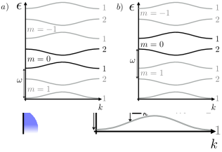
Despite the formal similarity to undriven systems, there are several fundamental differences between a Floquet effective Hamiltonian and a static Hamiltonian. First, there is an ambiguity in the definition of above: the quasienergies are only defined modulo multiples of the driving frequency . In other words, the definition of is invariant under the gauge transformation
| (3) |
for any set of integers . This makes an a priori definition of a “lowest” quasienergy impossible, since one can always fold and/or reorder (c.f. Fig. 1) the spectrum by means of such a gauge transformation Kohn (2001).
This obstruction to defining a unique Floquet ground state highlights a second important contrast with static systems, namely the fact that there is no universal principle determining the occupations of quasienergy states at zero temperature. Indeed, this signature of the inherently out-of-equilibrium nature of periodically-driven systems poses a challenge to theoretical proposals of Floquet topological states — even if a Floquet system has topological quasienergy bands, there is no guarantee that the long-time state of the system is a pure Floquet state with the desired features moo ; Dehghani et al. (2014); deh . For open systems in contact with a thermal reservoir, as is the case in solid-state realizations, the detailed properties of the reservoir and its coupling to the system play crucial roles in determining the nonequilibrium steady state of the system at long times gri ; Kohler et al. (1997); Breuer et al. (2000); Kohler et al. (2005); Kohn (2001); Hone et al. (2009); gra ; see .
In this work, we investigate the occupations of topological Floquet bands in a noninteracting fermionic system coupled to a thermal reservoir at zero temperature. We ask whether, and under what conditions, it is possible for the nonequilibrium steady state of the system to feature a single fully populated Floquet band when the original undriven system is half-filled. Using a Floquet master equation approach, we examine as a function of the driving amplitude and frequency the rate to escape a given Floquet state. We find that generic systems undergo heating that spoils the complete occupation of a single band, even in the favorable limit of weak, off-resonant driving. In the best-case scenario, the excitation density falls off as a power law in , with the non-universal decay exponent set by the low-energy behavior of the bath density of states. We close by suggesting bath engineering schemes that could further suppress excitations. While our motivation derives from the pursuit of topological phases in driven systems, we point out that our results hold equally well in “trivial” Floquet band insulators.
The structure of the paper is as follows. In Sec. II, we provide an overview of the Floquet master equation approach used in this work. Rather than focusing on exposition, this section provides a fresh perspective on the subject by emphasizing the requirement of invariance of all physical quantities under gauge transformations of the form (3). This physical principle resolves many of the conceptual ambiguities regarding the definitions of Floquet states and the associated quasienergies. Within this formalism, we outline conditions under which open Floquet systems can reach steady states that resemble their equilibrium counterparts, i.e. where the occupations of the Floquet states at finite temperature are distributed in a Boltzmann-like fashion. In the remaining sections, which can be read independently of Sec. II, we specialize to the study of noninteracting, two-band Floquet systems coupled to zero-temperature bosonic reservoirs, and present the main results of this work, which were outlined above.
II Floquet master equations
II.1 Definitions and comments on gauge invariance
In this paper, we will study Floquet systems that are described by Hamiltonians of the form
| (4) |
where describes the periodically driven system, describes the reservoir (or “bath”), and describes the coupling between them. Following Refs. Kohn, 2001 and Hone et al., 2009, we assume a system-bath coupling of the factorized form
| (5) |
where is a real coupling constant [assumed to be smaller than any energy scale in ], and where and are Hermitian operators acting solely on the degrees of freedom of the system and the bath, respectively foo (a). System-bath couplings of this form are ubiquitous in the study of open quantum systems, e.g. in spin-boson-type models Leggett et al. (1987). The reservoir described by , whose eigenstates and energies are known, is assumed to be in thermal equilibrium (either at zero temperature or at a finite temperature , although in Sec. III we will specialize to the case of zero temperature).
The unitary time evolution of the full closed system is completely characterized by the density matrix , whose equation of motion is given by
| (6) |
Our interest, however, is primarily in the influence of the reservoir on the system described by . The important quantity to consider is then the reduced density matrix
| (7) |
where represents the operation of taking the trace over the bath degrees of freedom. The evolution of the open system described by is obtained by “tracing out” the bath in Eq. (6), which results in a master equation for the reduced density matrix. Owing to the explicit time-dependence of , this master equation has time-periodic coefficients, so that the Floquet states defined by Eq. (1) form a natural basis in which to resolve gri ; Kohler et al. (1997); Breuer et al. (2000); Kohler et al. (2005); Kohn (2001); Hone et al. (2009). The derivation of the master equation for the reduced density matrix in the Floquet basis proceeds via the Born-Markov approximation, which amounts to an assumption of weak coupling between the system and bath, as well as the assumption that the correlation time of the bath is sufficiently short that memory effects can be neglected.
A particularly clear derivation of this Floquet master equation, as well as a careful discussion of the hierarchy of time-scales necessary in order for the Born-Markov approximation to hold, is presented by Hone et al. in Ref. Hone et al., 2009. We refer the reader to that work (and references therein) for details, and begin our discussion with the master equation written in their notation:
| (8a) | ||||
| where | ||||
| (8b) | ||||
| (8c) | ||||
| and the coefficients , where | ||||
| (8d) | ||||
| The influence of the bath is contained in the function , essentially a weighted density of states, which is defined by | ||||
| (8e) | ||||
| (8f) | ||||
where is the inverse temperature.
Equation (8) is advantageous in that it is completely invariant under the gauge transformations (3) that reshuffle the quasienergy spectrum. Indeed, defining
| (9a) | ||||
| (9b) | ||||
one finds that the density matrix transforms as
| (10) |
while the time-dependent rates transform as
| (11) |
Consequently, the left- and right-hand sides of Eq. (8) transform with an oscillating phase factor that cancels, and the equation is therefore invariant under the gauge transformation.
Despite the appeal of a gauge-invariant equation of motion for the reduced density matrix, it is also difficult to make analytical progress while the rates are time-dependent. If one is only interested, as we are, in the long-time limit, where the density operator does not vary substiantially over a single period, then a valid means of bypassing this difficulty is to consider the time-average of both sides of Eq. (8) Hone et al. (2009),
| (12a) | ||||
| where is the time-average of , and where | ||||
| (12b) | ||||
are the time-averaged rates. Equation (12a) can be further simplified by considering the structure of the averaged density matrix . Indeed, so long as for , the system-bath coupling can be chosen to be much smaller than the smallest . In this case, the off-diagonal elements of the steady-state reduced density matrix vanish to order (c.f. Hone et al. (2009)), and the occupations of the Floquet states are solutions to the rate equation
| (13) |
where the transition rates
| (14) | |||||
Our treatment of nonthermal steady states in Sec. III will be based on a careful analysis of the rate equation (13) in the special case of a two-state system.
The time-averaging process outlined above spoils the gauge-invariance of Eq. (8); after time-averaging, one therefore implicitly commits to a choice of ordering for the quasienergies. Indeed, observe that
| (15) | ||||
In particular, if . This indicates that the primed version of Eq. (12a) need not hold given the unprimed version. However, observe that the diagonal rates , along with the diagonal density matrix elements , are invariant under the gauge transformation (9) [c.f. Eq. (10)]. Therefore, the rate equation (13) that governs the steady-state populations is gauge invariant.
One important consequence of the gauge invariance of Eq. (13) is that, in addition to exact degeneracies where , one must also treat carefully quasi-degeneracies, where for some . Such situations were of primary concern in Ref. Hone et al., 2009, which points out that such degeneracies can have profound effects on the steady-state density matrix. In the language of gauge-invariance adopted here, such quasi-degeneracies are simply indicative of the fact that there exists a gauge in which quasienergies and are degenerate.
Consequently, in such situations, Eq. (13) is no longer valid in the basis of Floquet states. However, the density matrix nevertheless has a block-diagonal structure, being nonzero only when in some gauge. (Let us, for simplicity, adopt this gauge here and for the remainder of the present discussion.) To close this section, we show that a rate equation of the form (13) is recovered upon transforming to the basis in which is diagonal. The unitary transformation that diagonalizes the density matrix acts on the Floquet states as
| (16a) | ||||
| (16b) | ||||
| (16c) | ||||
| (16d) | ||||
We now plug these transformed quantities into Eq. (12a), keeping in mind that its left-hand side can be set to zero given that is zero whenever . We obtain, for each and ,
| (17) |
One can show that Eq. (II.1) holds if and only if
| (18) |
for all and . Next, consider the above equation when , while at the same time keeping in mind that is diagonal. We obtain
| (19) |
or equivalently
| (20) |
where is the probability of being in the state labeled by , and
| (21) |
This discussion has therefore demonstrated that a rate equation of the form (13) always determines the steady-state reduced density matrix in some basis, namely the basis in which is diagonal. Whether or not this basis is the basis of Floquet states, or some other time-periodic basis, depends on the degeneracy structure of the quasienergy spectrum. Nevertheless, the subsequent analyses presented here hold equally well in this choice of basis.
II.2 Conditions for thermal Floquet steady states
In this section, we will determine, within the master equation formalism discussed above, conditions under which the driven system relaxes to a thermal distribution with respect to the quasienergies. In particular, we will show that such a situation occurs provided that , where is defined via Eq. (2) with , is either time-independent or depends on time in a particularly simple way. While statements to this effect have been made in various works Iadecola et al. (2013a, b); Shirai et al. (2015); Liu (2015), we provide here a simple and complementary derivation of the statement from the master equation formalism outlined in Ref. Hone et al. (2009), and provide connections to the principle of gauge invariance discussed previously. Before beginning with the derivation, we observe that, at finite temperature, the function , which contains the influence of the bath on the driven system, satisfies
| (22) |
which induces the following generalized detailed balance relation for the rates appearing in Eq. (13) Hone et al. (2009):
| (23a) | |||
| where | |||
| (23b) | |||
Note that substituting Eq. (23) into the rate equation (13) yields a thermal distribution for the occupations of the Floquet states, i.e. if .
We can now show that such a thermal distribution emerges if is time-independent, simply by showing that it implies that only the terms contribute to Eq. (23). To do this, we make use of an explicit representation of the operator , which can be derived as follows. Noting first that the evolution operator can be written in terms of the Floquet states as
| (24) | ||||
we compute
| (25) | ||||
Acting from the right with on both lines above and using the fact that at any time , we deduce that
| (26) |
At this point, making the ansatz
| (27) |
we find that indeed
| (28a) | |||
| where | |||
| (28b) | |||
as desired.
Using the explicit form of provided in Eq. (27), the desired result follows directly from the definition of given in Eq. (23b). In particular, observe that
| (29) | ||||
If [and therefore ] is independent of time, then for all . We have therefore shown that, if the operator is time-independent, then the steady-state occupations of the Floquet states are given by , as they would be for a system with Hamiltonian at equilibrium with a finite-temperature reservoir. The zero-temperature limit of the associated grand-canonical distribution determines an unambiguous ordering of the quasienergies.
If is not time-independent, it is still possible to reach an effective thermal distribution if detailed balance, namely the relation
| (30) |
holds for all and . For example, let us expand the time-periodic operator , and consider the case where , for fixed and , is nonzero for a single mode . In this case,
| (31) | ||||
Since is a Hermitian operator, we have , and . It follows that Eq. (23) becomes
| (32) |
In this case, one recovers a thermal quasienergy distribution only if it is possible to consistently absorb the extra factor of into a redefinition of the quasienergies . In principle, this can be achieved by means of gauge transformations of the form (9), which shift the quasienergies by integer multiples of the driving frequency . In practice, however, it might arise that such a gauge transformation cannot be performed consistently over all Floquet states. Fortunately, there is a condition, demonstrated below, on the integers that guarantees that such a transformation can be carried out.
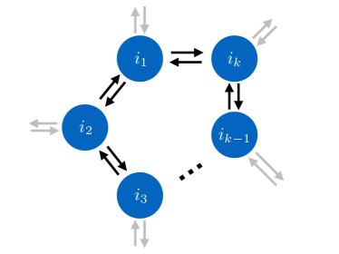
The set of nonvanishing transition rates defines the directed edges of a graph whose vertices are the Floquet states (see Fig. 2). In order to consistently gauge away the extra factor of , it is sufficient to require that for any closed loop in this graph, one has
| (33) |
[Observe that this condition holds automatically if detailed balance, Eq. (30), holds.] Using Eq. (32), one finds that this condition holds if and only if
| (34) |
which is the desired condition on the . The above condition is satisfied if for all and . [Note, however, that this condition is sufficient but not necessary to satisfy Eq. (34).] In this case, one can redefine the quasienergies via the gauge transformation
| (35a) | ||||
| such that Eq. (32) becomes | ||||
| (35b) | ||||
which yields the desired thermal quasienergy distribution .
III Zero-temperature nonequilibrium steady states
In this section, we carry out the program outlined in the introduction, and characterize the zero-temperature occupations of Floquet bands in a generic class of periodically-driven noninteracting systems. We take the combined Hamiltonian for the system and the reservoir to be given by Eq. (4), i.e.
| (36a) | |||
| The Hamiltonian describes the periodically-driven system, which we take for simplicity to be a two-band model of noninteracting fermions. (Generalizing our results to models with more than two bands is straightforward.) We will focus on the case of monochromatic driving, so that | |||
| (36b) | |||
| where is the driving amplitude and depends on time via linear combinations of and . The quasienergy bands of the driven system, denoted by (), are assumed to be gapped (i.e. nondegenerate for all ) and to host nontrivial topological invariants. The system-bath coupling is again taken to be in the factorized form of Eq. (5), namely | |||
| (36c) | |||
We also take the operator to conserve both momentum and particle number, so that each mode is effectively coupled to its own bath, and so hereafter we suppress the momentum index . Finally, describes a bosonic bath, with energy eigenstates and eigenvalues , which we take to be in equilibrium at zero temperature for all time.
If the Floquet spectrum is nondegenerate, as we assume, then is diagonal at long times, and the steady-state occupation probabilities , where , satisfy the rate equation (13), i.e.
| (37) |
We recall that the transition rates are defined as
| (38a) | ||||
| (38b) | ||||
| At zero temperature, the weighted bath density of states defined in Eq. (8e) is given by | ||||
| (38c) | ||||
We have set the bath ground-state energy , so that is strictly positive. For this reason, vanishes identically at zero temperature, a fact that will be of crucial importance below. In our analysis, it will be instructive to model as a power law at low energies compared to a very large cutoff scale Leggett et al. (1987):
| (39) |
The real exponent classifies the type of bath; if , the bath is referred to as ohmic, while and are referred to as super-ohmic and sub-ohmic, respectively.
It is interesting to note, as pointed out in Sec. II.1, that the rates entering equation (37) are invariant under gauge transformations of the form (3). While these gauge transformations change the ordering of the quasienergies, they nevertheless do not change the occupations of the Floquet states themselves. However, as we will see later on, an appropriately engineered reservoir is capable of determining an unambiguous ordering of the quasienergies and a choice of an effective “Floquet ground state.”
We now turn to an analysis of the transition rates (38a) that will allow us to determine the extent to which a single Floquet state can be populated at zero temperature, given that the system is coupled to a bath. For this analysis, it will be convenient to choose a gauge in which the ordering of the quasienergies is determined by the ordering of the energies of the undriven Hamiltonian , in such a way that the separation is positive. This gauge can be understood by building up the Floquet states perturbatively in from the eigenbasis of Sambe (1973). To do this, we make use of the Fourier decomposition of the time-periodic Floquet states,
| (40) |
and observe that, to zeroth order in this gauge, is nothing but an eigenstate of . (Notice also that are the eigenstates of underlying the Floquet topological insulator.) The nonzero- Fourier components of arise due to hybridization of the spectrum via , and therefore scale with the driving amplitude as
| (41) |
which follows within perturbation theory to -th order in foo (b). Henceforth, we will take to be small either on account of a small or a large . In the Appendix, we examine the case where is not small, which is much less favorable for Floquet topological states. Factoring out the scaling from the states , we find that one can rewrite the matrix elements in Eq. (38b) in the following form:
| (42) | ||||
where are regular functions containing the terms in the series that depend weakly on or lead to a decay of faster than as .
With all this in mind, we now analyze the quantity
| (43) |
which is proportional to the density of excitations above the “lowest” quasienergy state in this gauge (). If only above contributes, the excitation density vanishes and the lower band is completely filled at long times, as it would be at equilibrium, owing to the fact that the argument of in the numerator is positive. While model systems that reach such an effective equilibrium steady state have been studied Breuer et al. (2000); Iadecola et al. (2013b); Iadecola et al. (2014); Shirai et al. (2015); Liu (2015), it is well-known that these steady states do not occur for generic choices of and . We ask, instead, whether there are any more general mechanisms or limits that suppress . The analysis is simplified if we assume that is sufficiently small that we can keep only the lowest nontrivial value of in the sums above. We will focus on the case , since the opposite case would likely not yield a topological band structure.
For , then only the terms with () contribute to the numerator (denominator) of Eq. (43). In this case, we find that suppression of is possible in the limit , which yields [c.f. Eq. (42)]
| (44) |
In addition to the exponent , the behavior of as depends on the scaling of the quasienergy separation with and . We assume the scaling , for ; for example, the case corresponds to the size of the direct gap predicted in graphene coupled to a circularly polarized electric field Oka and Aoki (2009); Kitagawa et al. (2011). We additionally allow the driving amplitude to scale with the frequency, , as it may in some physical driven systems buk ; Aidelsburger et al. (2013). Using these scaling forms, we find that as the excitation density
| (45a) | |||
| so long as the product | |||
| (45b) | |||
| Noting that the simultaneous requirement of small and large restricts , this criterion reduces to | |||
| (45c) | |||
If this condition is not satisfied, then approaches a nonuniversal constant in the high-frequency limit, and no single Floquet state is fully populated in the steady state. It is important to note that , and therefore the excitation density, is -dependent, since the scaling of with varies in momentum space. In particular, for far away from the value at which the minimal quasienergy separation occurs, becomes independent of and . The -scaling for this case is obtained by setting in Eqs. (45).
For a given and (fixed by the physical realization of the system), the above result suggests that the low-energy behavior of the function essentially determines whether or not a single Floquet band is occupied in the limit . For example, in the case of graphene in a circularly-polarized electric field (, ), there is a critical value (i.e., ohmic dissipation) that separates the power-law decay of from the aforementioned nonuniversal behavior. Therefore, an ohmic bath already violates Eq. (45c) for graphene in a circularly-polarized electric field, and the population of the bands near the -point is not controllable by increasing if the bath is ohmic.
In cases where the excitation density decays as a power law at large frequencies, one must still take care to determine whether the resulting steady state has the desired characteristics of the topological Floquet bands. As increases, the Floquet effective Hamiltonian may approach as or faster. If the power-law decay of is faster than this approach, then the suppression of excitations can still occur in a regime where the Floquet bands are topological. The situation can be improved by allowing a scaling of the amplitude for buk , but the value of the exponent must be balanced against an appropriate value of [c.f. Eq. (45c)] in order for the desired suppression to take place. Furthermore, it is important to keep in mind that, depending on the exponents and , the power law decay of can be very slow, so that a finite density of excitations remains even at high frequencies compared to all system energy scales. In order for excitations to be completely suppressed, one must have
| (46a) | |||
| where the frequency- and momentum-dependent effective temperature is defined as | |||
| (46b) | |||
Note that this effective temperature arises even though the bath itself is at zero temperature, and can therefore be understood as a signature of heating effects due to the driving.
IV The role of bath engineering
The sensitive dependence on the exponent of the large-frequency scaling of the excitation density already demonstrates the crucial role that the bath plays in stabilizing Floquet topological states in open systems. We close by commenting on two additional ways in which the bath and its coupling to the system can be engineered in order to further favor the suppression of .

One way to suppress excitations is to engineer the spectrum of the bath itself so that the function appearing in Eq. (38a) does not have a simple power-law form as in Eq. (39), but instead drops to zero in a neighborhood of , where is some reference value of the quasienergy separation, as in Fig. 3. (Such a scenario could be envisioned if, for example, the bath consists of quantized electromagnetic radiation in a cavity, whose size could be tuned to achieve the desired effect.) If the width of the dip in is on the order of the width of the upper band, then excitations can be suppressed even if is not much larger than . Indeed, if and is sufficiently small that only the first few terms in the sums over in Eq. (43) are kept, then the suppression of near this value eliminates the terms with up to order . However, it is important to point out that the excitation density in this case still exhibits at best power-law decay at large frequencies, with appropriate modifications to Eqs. (45) arising from keeping terms other than in Eq. (43). To completely eradicate excitations to all orders in , one must engineer dips at energies for all .
Of course, by placing the dip at , one can also use this mechanism to populate what we have referred to as the upper band in this choice of gauge. While this scenario looks like a population inversion, one can of course perform an appropriate transformation of the form (3) to reorder the Floquet bands in such a way that the populated band is the lowest. This example indicates that, in certain cases, the reservoir can “choose” a preferred gauge in which the system appears to be (nearly) at equilibrium.
The system-bath coupling is another quantity that could potentially be manipulated in order to suppress excitations. Indeed, certain system-bath couplings are known to yield relaxation to steady states that feature filled Floquet bands. For example, if is chosen in such a way that , where satisfies Eq. (2) with , is time-independent, then the system described by the total Hamiltonian defined in Eq. (4) reaches an effective thermal equilibrium with respect to the eigenvalues of (see Sec. II.2 and Refs. Iadecola et al. (2013a, b); Shirai et al. (2015); Liu (2015)). Given sufficient control over the system-bath coupling, one could attempt to engineer such a situation, at least to some order in , by designing an that, say, commutes with the lowest nontrivial Fourier harmonic of , or even by engineering an appropriate time dependence in to cancel the time-dependence in to some order.
V Summary and Conclusion
We have argued in this work that the possibility of stabilizing a Floquet topological state with a low density of excitations is heavily constrained by the coupling to a thermal reservoir. Using scaling arguments, we demonstrated that, even in the limit of weak driving and/or high frequenscy, the bath density of states has tremendous influence on whether or not excitations are suppressed as . We also suggested ways of designing the bath and its coupling to the system in order to suppress excitations.
Our results suggest that it is at best difficult, and at worst impossible, to engineer a periodically-driven quantum system whose steady state resembles the zero-temperature ground state of some target topological phase. However, even out of equilibrium, there is reason to believe that nontrivial features, such as topological indices d’a , edge states moo , and (approximately) quantized transport deh ; Foa Torres et al. (2014), survive in both isolated and open systems. Indeed, there is already experimental evidence to this effect in cold atomic gases Aidelsburger et al. (2013); Jotzu et al. (2014). We emphasize, however, that it is precisely in the deviations from the resemblance to equilibrium systems where the newest physics lies. For example, interacting versions of these models Grushin et al. (2014) could be used as platforms to probe fractionalized excitations out of equilibrium.
Acknowledgments
We thank Camille Aron and Garry Goldstein for inspiring discussions. T.I. was supported by the National Science Foundation Graduate Research Fellowship Program under Grant No. DGE-1247312. T.N. was supported by DARPA
SPAWARSYSCEN Pacific N66001-11-1-4110, and C.C. was supported by DOE Grant DEF-06ER46316.
Note added — During preparation of this manuscript, we became aware of Ref. see, , which also discusses the possibility of stabilizing Floquet topological states with couplings to particular appropriately-engineered baths.
*
Appendix A Limit of strong driving
In the case of strong driving (), there are many values of for which can be non-negligible. Indeed, as , the Floquet states can become chaotic, so that the may be regarded as essentially random variables, whose magnitudes need not decay quickly as becomes large. For this reason, the sums in the numerator and denominator of Eq. (43) generically diverge in the limit , and the ratio of transition rates is indeterminate. One can, however, identify constraints on the amplitudes such that the ratio converges to a definite finite value. In particular, if
| (A1) |
as for any positive real number , then both series are bounded from above by a convergent series, and therefore the ratio has a definite value. This is true even for infinitesimally small .
Even if the sums in the numerator and denominator are divergent, the ratio (43) can approach a finite value for system-bath coupling operators such that , due to a symmetry. To see this, let us drop the term in the denominator and rewrite Eq. (43) for as
| (A2) |
For large , the summands in the numerator and denominator become identical. Therefore, if is finite for sufficiently large , the ratio of the two sums approaches 1 from below as grows. When this occurs, the system approaches an infinite effective temperature — all Floquet states are occupied with equal probabilities, despite the fact that the bath is held at zero temperature. If there exists some such that , then the ratio takes on a finite value that is bounded from above by unity.
References
- Oka and Aoki (2009) T. Oka and H. Aoki, Phys. Rev. B 79, 081406 (2009).
- Lindner et al. (2011) N. H. Lindner, G. Refael, and V. Galitski, Nature Phys. 7, 490 (2011).
- Kitagawa et al. (2011) T. Kitagawa, T. Oka, A. Brataas, L. Fu, and E. Demler, Phys. Rev. B 84, 235108 (2011).
- Gu et al. (2011) Z. Gu, H. A. Fertig, D. P. Arovas, and A. Auerbach, Phys. Rev. Lett. 107, 216601 (2011).
- Rudner et al. (2013) M. S. Rudner, N. H. Lindner, E. Berg, and M. Levin, Phys. Rev. X 3, 031005 (2013).
- Grushin et al. (2014) A. G. Grushin, A. Gómez-León, and T. Neupert, Phys. Rev. Lett. 112, 156801 (2014).
- Kundu et al. (2014) A. Kundu, H. A. Fertig, and B. Seradjeh, Phys. Rev. Lett. 113, 236803 (2014).
- Foa Torres et al. (2014) L. E. F. Foa Torres, P. M. Perez-Piskunow, C. A. Balseiro, and G. Usaj, Phys. Rev. Lett. 113, 266801 (2014).
- (9) J. P. Dahlhaus, B. M. Fregoso, and J. E. Moore, arXiv:1408.6811 (unpublished).
- Shirley (1965) J. H. Shirley, Phys. Rev. 138, B979 (1965).
- Sambe (1973) H. Sambe, Phys. Rev. A 7, 2203 (1973).
- Rahav et al. (2003) S. Rahav, I. Gilary, and S. Fishman, Phys. Rev. A 68, 013820 (2003).
- Goldman and Dalibard (2014) N. Goldman and J. Dalibard, Phys. Rev. X 4, 031027 (2014).
- (14) M. Bukov, L. D’Alessio, and A. Polkovnikov, arXiv:1407.4803 (unpublished).
- Hasan and Kane (2010) M. Z. Hasan and C. L. Kane, Rev. Mod. Phys. 82, 3045 (2010).
- Kohn (2001) W. Kohn, J. Stat. Phys. 103, 417 (2001).
- Dehghani et al. (2014) H. Dehghani, T. Oka, and A. Mitra, Phys. Rev. B 90, 195429 (2014).
- (18) H. Dehghani, T. Oka, and A. Mitra, arXiv:1412.8469 (unpublished).
- (19) M. Grifoni and P. Hänggi, Phys. Rep. 304, 229 (1998).
- Kohler et al. (1997) S. Kohler, T. Dittrich, and P. Hänggi, Phys. Rev. E 55, 300 (1997).
- Breuer et al. (2000) H.-P. Breuer, W. Huber, and F. Petruccione, Phys. Rev. E 61, 4883 (2000).
- Kohler et al. (2005) S. Kohler, J. Lehmann, and P. Hänggi, Phys. Rep. 406, 379 (2005).
- Hone et al. (2009) D. W. Hone, R. Ketzmerick, and W. Kohn, Phys. Rev. E 79, 051129 (2009).
- (24) T. Iadecola and C. Chamon, arXiv:1412.5599 (unpublished).
- (25) K. I. Seetharam, C.-E. Bardyn, N. H. Lindner, M. S. Rudner, and G. Refael, arXiv:1502.02664 (unpublished).
- foo (a) The alternative choice , which is sufficiently general to include couplings to phonons and fermionic leads, results only in cosmetic changes to the resulting kinetic equations; we therefore opt instead for the simpler form in Eq. (5).
- Leggett et al. (1987) A. J. Leggett, S. Chakravarty, A. T. Dorsey, M. P. A. Fisher, A. Garg, and W. Zwerger, Rev. Mod. Phys. 59, 1 (1987).
- Iadecola et al. (2013a) T. Iadecola, D. Campbell, C. Chamon, C.-Y. Hou, R. Jackiw, S.-Y. Pi, and S. V. Kusminskiy, Phys. Rev. Lett. 110, 176603 (2013a).
- Iadecola et al. (2013b) T. Iadecola, C. Chamon, R. Jackiw, and S.-Y. Pi, Phys. Rev. B 88, 104302 (2013b).
- Shirai et al. (2015) T. Shirai, T. Mori, and S. Miyashita, Phys. Rev. E 91, 030101 (2015).
- Liu (2015) D. E. Liu, Phys. Rev. B 91, 144301 (2015).
- foo (b) Note that one cannot rule out the possibility that scales with an additional nonuniversal function of that approaches unity as .
- Iadecola et al. (2014) T. Iadecola, T. Neupert, and C. Chamon, Phys. Rev. B 89, 115425 (2014).
- Aidelsburger et al. (2013) M. Aidelsburger, M. Atala, M. Lohse, J. Barreiro, B. Paredes, and I. Bloch, Phys. Rev. Lett. 111, 185301 (2013).
- (35) L. D’Alessio and M. Rigol, arXiv:1409.6319 (unpublished).
- Jotzu et al. (2014) G. Jotzu, M. Messer, R. Desbuquois, M. Lebrat, T. Uehlinger, D. Greif, and T. Esslinger, Nature 515, 237 (2014).