Group-galaxy correlations in redshift space as a probe of the growth of structure

Abstract

We investigate the use of the cross-correlation between galaxies and galaxy groups to measure redshift-space distortions (RSD) and thus probe the growth rate of cosmological structure. This is compared to the classical approach based on using galaxy auto-correlation. We make use of realistic simulated galaxy catalogues that have been constructed by populating simulated dark matter haloes with galaxies through halo occupation prescriptions. We adapt the classical RSD Dispersion model to the case of the group-galaxy cross-correlation function and estimate the RSD parameter $\beta$ by fitting both the full anisotropic correlation function $\xi^{s}(r_{p},\pi)$ and its multipole moments. In addition, we define a modified version of the latter statistics by truncating the multipole moments to exclude strongly non-linear distortions at small transverse scales. We fit these three observable quantities in our set of simulated galaxy catalogues and estimate statistical and systematic errors on $\beta$ for the case of galaxy-galaxy, group-group, and group-galaxy correlation functions. When ignoring off-diagonal elements of the covariance matrix in the fitting, the truncated multipole moments of the group-galaxy cross-correlation function provide the most accurate estimate, with systematic errors below 3% when fitting transverse scales larger than $10\,h^{-1}{\rm Mpc}$. Including the full data covariance enlarges statistical errors but keep unchanged the level of systematic error. Although statistical errors are generally larger for groups, the use of group-galaxy cross-correlation can potentially allow the reduction of systematics while using simple linear or Dispersion models.

1 Introduction

Cosmological observations over the past 15 years have established that the Universe is undergoing a late-time phase of accelerated expansion (e.g. Riess et al. 1998; Perlmutter et al. 1999). This is most naturally explained with the presence of a ‘dark energy’, a fluid with negative pressure filling the entire Universe, which is currently indistinguishable from Einstein’s cosmological constant. Alternatively, however, one may consider reproducing observations by modifying the very nature of the gravitational equations of General Relativity (e.g. Carroll et al. 2004; Joyce et al. 2014). Geometrical probes such as the Cosmic Microwave Background (CMB), Baryon Acoustic Oscillations (BAO) and type 1a Supernovae (SN1a) constrain the expansion history $H(z)$, which however can be equally well fitted by both scenarios. This degeneracy between dark energy and a modification of standard gravity can only be lifted by dynamical probes looking at the growth of structure inside the Universe, which is directly linked to the underlying theory of gravity (Joyce et al. 2014).

The growth of cosmological structure induces galaxy peculiar velocities, i.e. coherent flows of galaxies towards matter overdensities. When redshifts are used to map galaxy positions, we are sensitive to such peculiar velocities, whose line-of-sight component combines with the cosmological redshift. As a result, the reconstructed spatial distribution of objects is distorted in the radial direction, what are referred to as redshift-space distortions (RSD). RSD can be quantified statistically in galaxy redshift surveys by modelling the corresponding anisotropy that can be measured in the two-point correlation function (2PCF) $\xi(\mathbf{r})$ or, correspondingly, in the power spectrum $P(\mathbf{k})$. In the linear regime, this effect is described in Fourier space by the Kaiser model (Kaiser 1987), or its equivalent in configuration space developed by Hamilton (1992). Such modelling is however complicated by the non-linear evolution of matter overdensities and velocities (see e.g. de la Torre & Guzzo 2012, and references therein).

On large scales we can still observe the linear, coherent flows tracing the growth of cosmological structure, which enhance the amplitude of two-point correlations. But small-scale motions are dominated by high-velocity galaxies in virialized structures, resulting from the dynamical evolution of the highest peaks in the density field. The resulting stretching effect in galaxy maps is commonly referred to as the Fingers of God effect (FoG), due to the elongated shapes that groups and clusters acquire when observed in redshift space. These two regimes of RSD produce characteristic features in the two-point statistics of the galaxy distribution, which can be studied by computing the correlation function as a function of two variables, $r_{p}$ and $\pi$, perpendicular and parallel to the line of sight, respectively. The two effects, linear and non-linear, introduce respectively a large-scale squashing and a small-scale elongation along the line-of-sight direction $\pi$. In linear theory, the amplitude of the squashing effect is directly proportional to the logarithmic growth rate of density fluctuations $f(z)$ (see Eq. (8)) (Kaiser 1987). In practice, our discrete tracers will generally be biased with respect to the overall matter distribution. Under the hypothesis of a linear bias $b_{\rm lin}(z)$, the large-scale squashing effect will depend on the parameter $\beta(z)\equiv f(z)/b_{\rm lin}(z)$.

An empirical correction to the linear model was introduced as to account for the contribution of nonlinear distortions, what is normally referred to as the Dispersion model (Fisher et al. 1994; Peacock & Dodds 1994). In this model, the linear expression is convolved (in configuration space), or multiplied (in Fourier space) with a given distribution function for the pairwise velocities $\varphi(v_{||})$ along the line of sight. The dispersion model has been widely and successfully used in the past to estimate $\beta(z)$ from measurements of $\xi(r_{p},\pi)$ (Peacock et al. 2001; Hawkins et al. 2003; Guzzo et al. 2008; Ross et al. 2007; Cabré & Gaztañaga 2009a, b; Contreras et al. 2013) or the power spectrum (Percival et al. 2004; Tegmark et al. 2004; Blake et al. 2011). It has become clear that such empirical correction provides estimates that can be biased by up to 10%, typically depending on the bias of the tracer being employed (Okumura & Jing 2011; Bianchi et al. 2012). The precision already achieved by current largest surveys requires to improve on these limitations to reach systematic errors of the order of the percent (e.g. BOSS, Reid et al. 2014; Beutler et al. 2014; Samushia et al. 2014; Sánchez et al. 2014; Alam et al. 2015). Such limitations are intrinsic in the empirical nature of the dispersion model (Scoccimarro 2004; de la Torre & Guzzo 2012) and significant effort has been invested over the past five years to improve this theoretical description (e.g. Scoccimarro 2004; Taruya et al. 2010; Reid & White 2011; de la Torre & Guzzo 2012, and references therein, Reid et al. 2014). Alternatively, these theoretical limitations may be evaded if we are able to (a) identify galaxy tracers that are less affected by non-linearities, and/or (b) build novel statistics of galaxy clustering for which model fits are less sensitive to the same effect, while keeping the theoretical model as simple as possible.

In this paper we investigate two options along these two avenues. Specifically, we consider the case in which one has access to a robust galaxy group catalogue within the volume of a corresponding galaxy redshift survey; this will be possible with next-generation galaxy redshift surveys such as Euclid (Laureijs et al. 2011), also in combination with observations in other bands, as in particular the X-ray data from e-Rosita (Merloni et al. 2012). We therefore first consider the merits of using the galaxy group-galaxy cross-correlation to extract the distortion parameter $\beta$. We might expect the centre of mass of a galaxy group to have little or no random velocity, since the internal orbital velocities produce Fingers-of-God only in the overall galaxy distribution. In this view, group-group correlations should be ideally placed (as also suggested by the dependence of the systematic error on the halo mass shown by Bianchi et al. 2012). Moreover, the group-galaxy cross-correlation provides a higher statistical power than using group auto-correlation, given the higher number density of the galaxy catalogue. Secondly, we investigate a new way of compressing the cosmological information present in the anisotropic two-point correlation function in redshift space, by building modified (truncated) multipole moments of $\xi(r_{p},\pi)$ that partially mitigate small-scale non-linearities. These functions avoid explicitly including the contributions from small transverse scales, dominated by non-linear distortions. In this analysis, we therefore compare the standard approach of using galaxy or group auto-correlation and the novel approach of using the galaxy-group cross-correlation, as well as study how the different estimators of the two-point statistics, namely the anisotropic 2PCF $\xi^{s}(r_{p},\pi)$, its standard multipoles $\xi^{s,(\ell)}(s)$ and its truncated multipoles $\hat{\xi}^{s,(\ell)}(s)$, behave in recovering the distortion parameter $\beta$ in simulations.

The paper is organized as follows. In Section 2, we derive the linear Kaiser/Hamilton and Dispersion models for the cross-correlation in the case of different observables: the anisotropic 2PCF $\xi^{s}(r_{p},\pi)$, its multipole moments $\xi^{s,(\ell)}(s)$, and the related truncated multipole moments $\smash{\hat{\xi}^{s,(\ell)}(s)}$. In section 3, we describe the data, two-point correlation function estimators, as well as ingredients needed to build theoretical models. In Section 4 we present the comparative analysis of the different approaches and methods. Finally, in Section 5 we discuss our results and conclude.

2 Redshift-Space Distortions: Modelling

The apparent positions of objects are modified if we use redshifts to infer cosmological distances. The line-of-sight component of the peculiar velocity distorts positions in the following way:

$$\mathbf{s}=\mathbf{r}+\mathbf{u}(\mathbf{r})\cdot\hat{\mathbf{e}}_{||},$$ (1)

where $\mathbf{s}$ and $\mathbf{r}$ are objects positions, respectively, in redshift- and real space; $\hat{\mathbf{e}}_{||}$ is the unit vector along the line of sight; $\mathbf{u}$ is the scaled velocity field defined as $\mathbf{u}(\mathbf{r})=\mathbf{v}(\mathbf{r})/aH(a)$ with $\mathbf{v}(\mathbf{r})$ being the peculiar velocity field; $a$ is the scale factor; and $H(a)$ is the expansion rate of the Universe. The $\mathbf{s}$ coordinates constitute the so-called redshift space and the distortions produced in the matter distribution are usually referred to as Redshift-Space Distortions (RSD).

2.1 Linear Model for the Cross-Correlation

We first derive the linear model for the two-point cross-correlation function. Following the derivation of Kaiser (1987) for the auto-correlation, we start with assuming mass conservation in real- and redshift space in terms of overdensities $\delta(\mathbf{r})=\rho(\mathbf{r})/\langle{\rho}\rangle-1$:

$$\left[1+\delta_{m}^{s}(\mathbf{s})\right]d^{3}\mathbf{s}=\left[1+\delta_{m}(\mathbf{r})\right]d^{3}\mathbf{r},$$ (2)

where $\delta_{m}(\mathbf{r})$ and $\delta_{m}^{s}(\mathbf{s})$ are, respectively, the matter density contrast in real- and redshift space. The volume element in redshift space $d^{3}\mathbf{s}$ is related to that in real space $d^{3}\mathbf{r}$ through $d^{3}\mathbf{s}=|J|d^{3}\mathbf{r}$ where $|J|$ is the Jacobian of the related coordinates transformation. In the particular case of the transformation in equation (1), the Jacobian is given by

$$|J|=1+\partial_{||}u_{||}(\mathbf{r}),$$ (3)

where $\partial_{||}=\partial/\partial r_{||}$ and $u_{||}(\mathbf{r})=\mathbf{u}(\mathbf{r})\cdot\hat{\mathbf{e}}_{||}$ is the line-of-sight component of the scaled velocity field $\mathbf{u}(\mathbf{r})$. Equation (2) can thus be written as

$$\delta_{m}^{s}(\mathbf{s})=\left[\delta_{m}(\mathbf{r})-\partial_{||}u_{||}(\mathbf{r})\right]\left[1+\partial_{||}u_{||}(\mathbf{r})\right]^{-1}.$$ (4)

In the linear regime approximation (i.e. small real-space density field $\left|\delta(\mathbf{r})\right|\ll 1$, small velocity gradients $\left|\partial_{||}u_{||}\right|\ll 1$ and an irrotational velocity field $\mathbf{\nabla}\!\times\!\mathbf{u}(\mathbf{r})=0$), equation (4) becomes

$$\delta_{m}^{s}(\mathbf{s})=\left[\delta_{m}(\mathbf{r})-\partial_{||}u_{||}(\mathbf{r})\right]\left[1-\partial_{||}u_{||}(\mathbf{r})\right].$$ (5)

Neglecting higher order terms in equation (5) gives

$$\delta_{m}^{s}(\mathbf{s})=\delta_{m}(\mathbf{r})-\partial_{||}u_{||}(\mathbf{r}).$$ (6)

In the plane parallel approximation, when the scales of perturbations are assumed to be much smaller then their distances from us (i.e. $u_{||}/r_{||}(\mathbf{r})\ll 1$), equation (6) can be written in Fourier space as

$$\delta_{m}^{s}(k,\mu_{k})=\left[1+f(z)\mu_{k}^{2}\right]\delta_{m}(k).$$ (7)

with $\mu_{k}=k_{||}/k$. In equation (7) $f$ is the growth rate of structure defined as:

$$f(a)=\frac{d\ln\delta_{m}(a)}{d\ln a}.$$ (8)

Equation (7) is valid for the overall matter density field. However, when objects of a given type $i$ are used as tracers of the overall matter density field, their distribution is in general biased with respect to the underlying matter. At first order, the overdensity $\delta_{i}$ of a given population $i$ can be related to that of the overall matter $\delta_{m}$ through a linear bias factor $b_{i}$

$$\delta_{i}(\mathbf{k})=b_{i}\,\delta_{m}(\mathbf{k}).$$ (9)

In this work we assume the linear bias $b_{i}$ to be a scale-independent parameter which is valid with good approximation in regimes that are not affected by small-scale non linearities and the ones due to the Baryon Acoustic Oscillations (BAO).

We also assume the peculiar velocity field of $i$-type objects to be unbiased with respect to that of the overall matter. This assumption holds on scales much larger than the typical size of virialized structures. Indeed, inside such structures dynamical processes such as dynamical friction and tidal disruption may alter the velocity field of objects $i$ with respect to that of the total matter introducing a further velocity bias (Munari et al. 2013; Elia et al. 2012). Thus, equation (7) becomes

$$\delta_{i}^{s}(k,\mu_{k})=\delta_{i}(k)+f(z)\,\mu_{k}^{2}\,\delta_{m}(k).$$ (10)

Defining the distortion parameter $\beta_{i}(z)$, related to the population $i$, as

$$\beta_{i}(z)=\frac{f(z)}{b_{i}(z)},$$ (11)

and combining it with equation (10) and the linear bias relation (9) leads to

$$\delta_{i}^{s}(k,\mu_{k})=\left[1+\beta_{i}(z)\mu_{k}^{2}\right]\delta_{i}(k).$$ (12)

Given two population of objects, e.g. individual galaxies ‘gal’ and their groups ‘gr’, their cross power spectrum is defined as

$$\left\langle\delta_{\rm gal}(\mathbf{k}_{1})\delta_{\rm gr}(\mathbf{k}_{2})\right\rangle=(2\pi)^{3}\delta_{D}(\mathbf{k}_{2}-\mathbf{k}_{1})P_{\rm cr}(\mathbf{k}).$$ (13)

The linear cross power spectrum in redshift space $P_{\rm cr,lin}^{(s)}(\mathbf{k})$ can be related to that in real space $P_{\rm cr}(\mathbf{k})$ by combining equation (13) with (12)

$$P_{\rm cr,lin}^{s}(k,\mu_{k})=\left[1+\beta_{\rm gal}\mu_{k}^{2}\right]\left[1+\beta_{\rm gr}\mu_{k}^{2}\right]P_{\rm cr}(k).$$ (14)

It is useful to write $P_{\rm cr,lin}^{s}(k,\mu_{k})$ as a sum of spherical harmonics

$$P^{s}_{\rm cr,lin}(k,\mu_{k})=\sum_{\ell}P_{\rm cr,lin}^{s,(\ell)}(k)L_{\ell}(\mu_{k}),$$ (15)

here, $L_{\ell}(\mu_{k})$ are the Legendre polynomials and $P_{\rm cr,lin}^{s,(\ell)}(k)$ are the multipole moments of the linear cross power spectrum $P_{\rm cr,lin}^{s}(\mathbf{k})$ given by

$$P_{\rm cr,lin}^{s,(\ell)}(k)=\frac{2\ell+1}{2}\int_{-1}^{+1}P_{\rm cr,lin}^{s}(k,\mu_{k})L_{\ell}(\mu_{k})d\mu_{k}.$$ (16)

The equivalent expression for the two-point cross-correlation function $\xi_{\rm cr,lin}^{s}(\mathbf{r})$ is provided by Hamilton (1992)

$$\xi_{\rm cr,lin}^{s}(r_{p},\pi)=\sum_{\ell}\xi_{\rm cr,lin}^{s,(\ell)}(s)L_{\ell}(\mu).$$ (17)

In equation (17), $r_{p}$ and $\pi$ are respectively the components of the pair separation $\mathbf{s}$ transverse and parallel to the line of sight, $\mu$ is the cosine of the angle between the pair separation $\mathbf{s}$ and the line of sight and $\xi_{\rm cr,lin}^{s,(\ell)}(s)$ are the multipole moments of $\xi_{\rm cr,lin}^{s}(r_{p},\pi)$:

$$\xi_{\rm cr,lin}^{s,(\ell)}(s)=i^{\ell}\int\frac{k^{2}dk}{2\pi^{2}}P_{\rm cr,lin}^{s,(\ell)}(k)j_{\ell}(ks),$$ (18)

where $j_{\ell}(ks)$ are the spherical Bessel functions. The only non-null multipole moments are

$$\xi_{\rm cr,lin}^{s,(0)}(s) =\left[1\!+\frac{1}{3}\!(\!\beta_{\rm gal}+\beta_{\rm gr})+\frac{1}{5}\beta_{\rm gal}\beta_{\rm gr}\right]\xi_{\rm cr}(r)$$ (19a)

$$\xi_{\rm cr,lin}^{s,(2)}(s) =\!\left[\!\frac{2}{3}(\!\beta_{\rm gal}\!+\!\beta_{\rm gr}\!)\!+\!\frac{4}{7}\beta_{\rm gal}\beta_{\rm gr}\!\right]\!\left[\xi_{\rm cr}(r)\!-\!\bar{\xi}_{\rm cr}(r)\right]$$ (19b)

$$\xi_{\rm cr,lin}^{s,(4)}(s) =\!\left[\!\frac{8}{35}\beta_{\rm gal}\beta_{\rm gr}\!\right]\left[\xi_{\rm cr}(r)\!+\!\frac{5}{2}\bar{\xi}_{\rm cr}(r)\!-\!\frac{7}{2}\bar{\bar{\xi}}_{\rm cr}(r)\right],$$ (19c)

where $\bar{\xi}_{\rm cr}(r)$ and $\bar{\bar{\xi}}_{\rm cr}(r)$ are the integrals of the real-space angle-averaged two-point cross-correlation function $\xi_{\rm cr}(r)$ (Cole et al. 1994):

$$\bar{\xi}_{\rm cr}(r) =\frac{3}{r^{3}}\int_{0}^{r}\xi_{\rm cr}(r^{\prime})r^{\prime 2}dr^{\prime}$$ (20a)

$$\bar{\bar{\xi}}_{\rm cr}(r) =\frac{5}{r^{5}}\int_{0}^{r}\xi_{\rm cr}(r^{\prime})r^{\prime 4}dr^{\prime}\,.$$ (20b)

This model was adopted by Mountrichas et al. (2009) to measure the bias of the QSOs in 2SLAQ, 2QZ and SDSS, by cross-correlating them with a population of Luminous Red Galaxies (LRG) in 2SLAQ and AAOmega.

Both $\beta_{\rm gal}$ and $\beta_{\rm gr}$ in fact describe the same growth rate $f\left(z\right)$; therefore using the linear bias relation (9), the 2PCF of the population $i$, in real space, can be written as

$$\xi_{i}(\mathbf{r})=b_{i}^{2}\xi_{m}(\mathbf{r}).$$ (21)

Combining equation (21), written separately for galaxies $\xi_{\rm gal}$ and groups $\xi_{\rm gr}$, with (11) gives

$$\beta_{\rm gr}(z)=b_{12}(z)\beta_{\rm gal}(z).$$ (22)

In equation (22), $b_{12}(z)$ is the ‘relative bias’ between galaxies and groups, defined as

$$b_{12}(z)=\left[\frac{\xi_{\rm gal}}{\xi_{\rm gr}}\right]^{1/2}=\frac{b_{\rm gal}(z)}{b_{\rm gr}(z)}.$$ (23)

This quantity can be estimated directly from the data, once the real-space correlation functions of the two populations are measured through projection of $\xi^{s}(r_{p},\pi)$. Defined in this way, $b_{12}$ will be smaller than unity, given the larger bias of groups with respect to galaxies. We prefer this definition as it allows us to obtain a more compact notation in the following equations. Using equation (22), therefore, equations (19a),(19b), (19c) become

$$\xi_{\rm cr,lin}^{s,(0)}(s) =\left[1\!+\frac{1}{3}\beta_{\rm gal}\!(\!1+b_{12})+\frac{1}{5}\beta_{\rm gal}^{2}b_{12}\right]\xi_{\rm cr}(r)$$ (24a)

$$\xi_{\rm cr,lin}^{s,(2)}(s) =\!\left[\!\frac{2}{3}\beta_{\rm gal}\!(\!1+b_{12})+\!\frac{4}{7}\beta_{\rm gal}^{2}b_{12}\!\right]\!\left[\xi_{\rm cr}(r)\!-\!\bar{\xi}_{\rm cr}(r)\right]$$ (24b)

$$\xi_{\rm cr,lin}^{s,(4)}(s) =\!\left[\!\frac{8}{35}\beta_{\rm gal}^{2}b_{12}\!\right]\left[\xi_{\rm cr}(r)\!+\!\frac{5}{2}\bar{\xi}_{\rm cr}(r)\!-\!\frac{7}{2}\bar{\bar{\xi}}_{\rm cr}(r)\right]\,.$$ (24c)

The linear Kaiser/Hamilton model for the two-point auto-correlation function is recovered just by taking $b_{12}(z)=1$ and replacing the real-space two-point cross-correlation function $\xi_{\rm cr}(r)$ and its integrals $\bar{\xi}_{\rm cr}(r)$, $\bar{\bar{\xi}}_{\rm cr}(r)$ with their counterparts in the auto-correlation case.

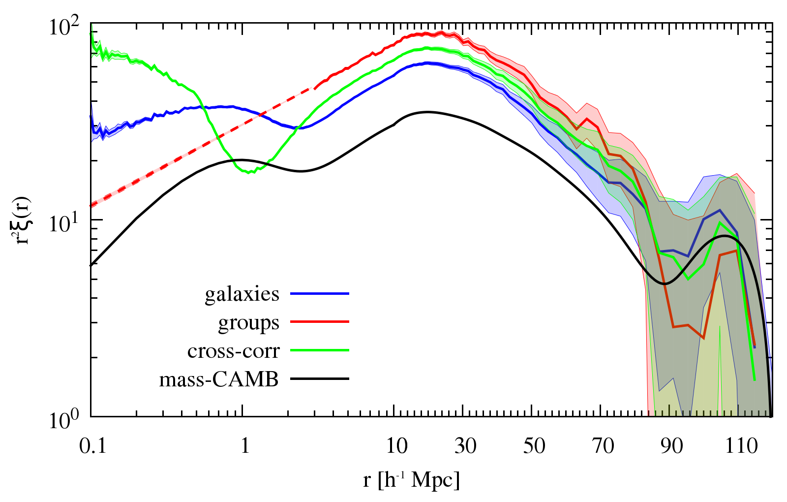
Figure 1: Real-space two-point correlation function measurements from the MultiDark Run1 data at $z=0.1$, averaged over 27 equal sub-samples. Blue line shows the (HOD, $L>1L^{*}$) galaxy auto-correlation, red line represents the auto-correlation of ($M>10^{13}h^{-1}M_{\odot}$ dark matter haloes) groups while the group-galaxy cross-correlation is plotted with green line. The CAMB model prediction for the correlation function of the underlying matter density field is also plotted (black line). The red dashed line is the power-law extrapolation of the group auto-correlation function on scales below $3\,h^{-1}{\rm Mpc}$ using parameters in Table 1. The relative statical errors on the averaged correlation functions are shown as the transparent filled contours.

2.2 The Dispersion Model

To derive the linear model in Section 2.1, strong assumptions have been made, limiting its validity to the very large scales.

We adopt the mostly used empirical ‘Dispersion model’ (Peacock & Dodds 1994) to model the shape of the 2PCF on small and intermediate trans-linear scales. This model convolves the linear model presented in Section 2.1 with a peculiar Pairwise Velocity Distribution (PVD) function along the line of sight $\varphi(v_{||})$:

$$\xi^{s}(r_{p},\pi)=\int_{-\infty}^{+\infty}\xi_{\rm lin}^{s}\left[r_{p},\pi-\frac{v_{||}}{aH(a)}\right]\varphi(v_{||})dv_{||}.$$ (25)

Different functional forms have been proposed in the literature for the PVD function. We adopt an exponential distribution function for $\varphi(v_{||})$ which is found to be in good agreement both with data from N-body simulations and with observations from large galaxy redshift surveys (Zurek et al. 1994):

$$\varphi(v_{||})=\frac{1}{\sqrt{2}\,\sigma_{12}}e^{-\frac{\sqrt{2}\,\left|v_{||}\right|}{\sigma_{12}}}.$$ (26)

Here, $\sigma_{12}$ is usually referred to as the peculiar pairwise velocity dispersion along the line of sight. In this paper we assume $\sigma_{12}$ to be a scale-independent free parameter. More complicated and accurate models for the peculiar pairwise velocity distribution have been calibrated on simulations to take into account the scale dependence of the velocity distribution (e.g. Zu & Weinberg 2013; Bianchi et al. 2014).

2.3 Truncated Multipole Moments

The standard multipole moments of the 2PCF $\xi^{s}(\mathbf{s})$ are obtained by projecting it onto the Legendre polynomials:

$$\xi^{s,(\ell)}(s)=\frac{2\ell+1}{2}\int_{-1}^{+1}\xi^{s}(s,\mu)L_{\ell}(\mu)d\mu,$$ (27)

with $s^{2}=r_{p}^{2}+\pi^{2}$ and $\mu=\pi/s$.

Since strong non-linear distortions affect small transverse $(r_{p})$ scales, we propose an alternative way of using the multipole moments of the 2PCF by removing such scales. This means that, at a given scale $s$, we consider only the clustering signal at $r_{p}>\bar{r}_{p}$. The new ‘multipole moments’ are then given by

$$\smash{\hat{\xi}^{s,(\ell)}(s)}=\frac{2\ell+1}{2}\int_{-\bar{\mu}}^{+\bar{\mu}}\xi^{s}(s,\mu)L_{\ell}(\mu)d\mu,$$ (28)

where

$$\bar{\mu}=\sqrt{1-\left(\frac{\bar{r}_{p}}{s}\right)^{2}}\,.$$ (29)

It is important to stress here that although $\smash{\hat{\xi}^{s,(\ell)}(s)}$ are not, mathematically speaking, the multipole moments of the 2PCF, in the following part, for the sake of simplicity, we will refer to them as the ‘truncated multipole moments’.

The gain in using the truncated multipole moments is given by the fact that they reconcile the classical approach of using the anisotropic 2PCF $\xi(r_{p},\pi)$ with the one of using its multipole moments. Indeed, the anisotropic 2PCF $\xi(r_{p},\pi)$ allows us to systematically exclude from the fit small transverse $r_{p}$ scales, affected by strong non-linear distortions, which are difficult to model analytically. However, this approach would involve a huge covariance matrix: it is thus in practice computationally infeasible. The size of the covariance matrix in the case of multipole moments is much smaller, but nonlinearities on small transverse scales make an undesired contribution when projecting the redshift-space 2PCF $\xi^{s}(s,\mu)$ onto the Legendre polynomials. The truncated multipoles allow us to remove these strong non-linear distortions, while retaining a relatively small covariance matrix and yielding a numerically tractable problem.

3 Methodology

To test the model presented in Section 2, we make use of simulated catalogues of galaxies and groups based on the MultiDark Run1 (MDR1) dark matter N-body simulation (Prada et al. 2012). MDR1 is a high mass resolution simulation within a cube of side $1000\,h^{-1}{\rm Mpc}$, with $N_{p}=2048^{3}$ dark matter particles and the mass of each particle being $M_{p}=8.721\times 10^{9}h^{-1}M_{\odot}$. It assumes a $\Lambda$CDM cosmology using cosmological parameters from WMAP5 and WMAP7 data releases $(\Omega_{m},\Omega_{\Lambda},\Omega_{b},n_{s},h,\sigma_{8})=(0.27,0.73,0.0469,0.95,0.7,0.82)$. Dark matter haloes in MDR1 are identified using the Friends-of-Friends (FoF) algorithm.

We use the simulated galaxy catalogue used in de la Torre & Guzzo 2012, which was constructed by populating MDR1 dark matter haloes and specifying the Halo Occupation Distribution (HOD). It contains 2,945,687 galaxies with a B-band luminosity of $L>L^{*}$. We used the HOD parametrization of Zheng et al. (2005) with parameters $(\log M_{min},\sigma_{\log m},\log M_{0},\log M_{1},\alpha)=(12.18,0.21,12.18,13.31,1.08)$ with masses given in units of $M_{\odot}/h$. The details of the HOD model that has been used and the construction of the sample are provided in Appendix B of de la Torre & Guzzo 2012. We only remark here that halos are assumed isotropic and spherical, with satellite galaxy velocities drawn from Gaussian distribution functions along each Cartesian direction, with dispersion computed following van den Bosch et al. (2004).

For the group catalogue, we use all dark matter haloes with mass $M>10^{13}h^{-1}M_{\odot}$ giving a total of 350,518 groups. This specific mass threshold is chosen as to match the observed number density of groups in the 2dFGRS Percolation-Inferred Galaxy Group (2PIGG) catalogue drawn from the 2dFGRS (Eke et al. 2004).

3.1 Estimator

We measure the 2PCF using the minimum variance estimator proposed by Landy & Szalay (1993) adapted to the case of cross-correlation function:

$$\xi_{LS}(\mathbf{s})=\frac{D_{1}D_{2}(\mathbf{s})-D_{1}R(\mathbf{s})-D_{2}R(\mathbf{s})+RR(\mathbf{s})}{RR(\mathbf{s})},$$ (30)

where $D_{1}D_{2}$ are the $data-data$ pairs between the two different catalogues, $D_{i}R$ are the $data_{i}-random$ pairs and $RR$ are the $random-random$ pairs. All pair counts are normalized to the related total numbers of distinct pairs.

Multipole moments of the measured two-point correlation function $\xi(\mathbf{s})$ are obtained by simply projecting it onto the Legendre polynomials (equation 31):

$$\xi^{s,(\ell)}(s)=\frac{2\ell+1}{2}\int_{-1}^{+1}\left[\frac{D_{1}D_{2}(s,\mu)-D_{1}R(s,\mu)-D_{2}R(s,\mu)+RR(s,\mu)}{RR(s,\mu)}\right]L_{\ell}(\mu)d\mu$$ (31)

To measure the truncated multipole moments, containing the clustering signal only on transverse scales $r_{p}>\bar{r}_{p}$, the integration in equation (31) is truncated at $\left[-\bar{\mu},+\bar{\mu}\right]$ rather than $\left[-1,+1\right]$ with $\bar{\mu}$ given by equation (29). We make use of a random catalogue with a number of random points 10 times larger than the galaxy sample to reduce the shot noise in our measurements.

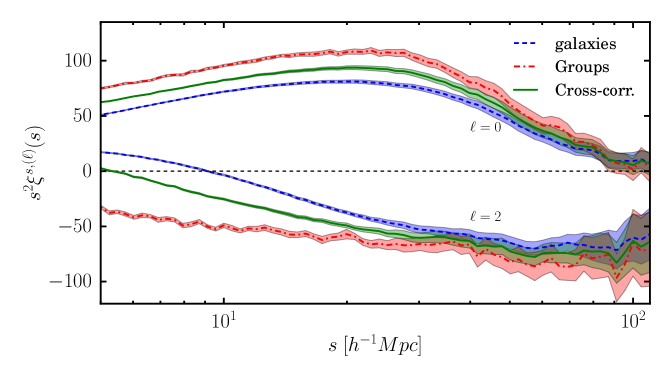
(a) Standard multipoles

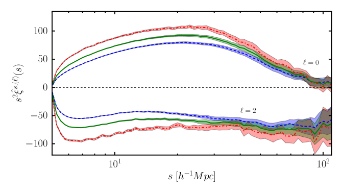
(b) Truncated multipoles

Figure 2: Standard (top panel) and truncated (bottom panel) monopole $\ell=0$ and quadrupole $\ell=2$ of the 2PCF in redshift space averaged among $N_{s}=27$ equal sub-volumes drawn from the MDR1 simulation at $z=0.1$. The blue dashed lines show the auto correlation of (HOD, $L>1L^{*}$ ) galaxies, red dash-dotted lines represent the group ($M>10^{13}h^{-1}M_{\odot}$ dark matter haloes) auto-correlation and their cross correlation is plotted with green continuous lines. The shaded regions show the related rms among $N_{s}$ measurements scaled by $1/N_{s}$.

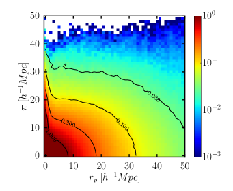
(a) Galaxies (HOD, $L>L*$)

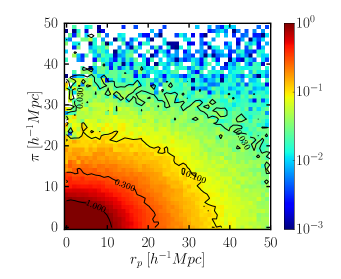
(b) Groups (Haloes $M>10^{13}h^{-1}M_{\odot}$)

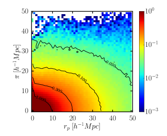
(c) Cross-correlation

Figure 3: Anisotropic two-point auto-correlation functions $\xi^{s}(r_{p},\pi)$ for galaxies (top left panel), groups (top right panel) and their cross-correlation (bottom panel) averaged among $N_{s}=27$ equal sub-volumes.

We use logarithmic $s$ bins of size $\Delta s_{log}=0.02$ that covers the range $\left[0.1,200\right]\,h^{-1}{\rm Mpc}$. $\mu$ is divided into $200$ linear bins between $\left[0,1\right]$. The measurements of the real-space correlation functions are shown in Figure 1, while the measured standard and truncated multipoles for the case of $\bar{r}_{p}=5\,h^{-1}{\rm Mpc}$ are shown in Figure 2. For the anisotropic 2PCF $\xi(r_{p},\pi)$, both transverse $r_{p}$ and parallel to the line-of-sight $\pi$ components of pair separation are linearly binned with bins of size $1\,h^{-1}{\rm Mpc}$ in the interval $\left[0,100\right]\,h^{-1}{\rm Mpc}$. The measured anisotropic 2PCF are presented in Figure 3.

$$\log_{10}(r_{i+1})=\log_{10}(r_{i})+s_{log}$$ (32)

Measurements in linear bins are sampled at the mid point of each bin while in the case of logarithmic binning a logarithmic average (eq. 33) of the two edges of each bin is taken as the reference point.

$$\log_{10}\langle r_{i}\rangle=\frac{\log_{10}r_{i}+\log_{10}r_{i+1}}{2}$$ (33)

In the last part of the analysis, we fix the number of bins in $s$ to $N_{b}=12$ inside the range $[s_{min},80]h^{-1}$Mpc in order to fit multipole moments with the full covariance matrix (see Section 3.2).

3.2 Error Covariance Matrix

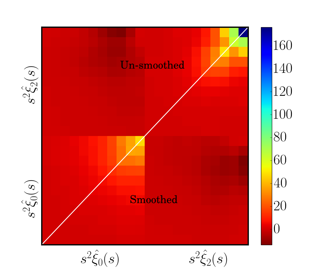
(a) Covariance matrix

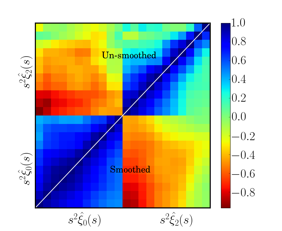
(b) Correlation matrix

Figure 4: Covariance (left panel) and correlation (right panel) matrices of the truncated multipoles of the two-point group-galaxy cross-correlation between $[5,80]h^{-1}$Mpc. In each panel the matrix above the white continuous line shows the direct measurement from $27$ equal sub-volumes while the lower part show the matrix after it has been smoothed using a box-car algorithm on $3\times 3$ sub-matrices (right panel).

In principle, the determination of the covariance matrix requires many independent realizations of our dataset, of which we inevitably possess only a single example. As an approximation to the ideal case, essentially two classes of methods have been proposed: (a) use simulated data, to produce $N_{r}$ independent mock samples with properties as close as possible to the observed data; (b) use internal methods, in which $N_{r}$ multiple realizations are constructed from the overall data, by resampling the observations in some appropriate way. In particular, four such methods have been used in the past literature: (1) the classical bootstrap method, in which each realization is constructed by resampling with replacement of single objects in the data set. In the other three methods, the sample volume is split into a number of sub-volumes, which are then combined following different schemes: (2) the block-wise bootstrap method builds realizations by combining all sub-volumes, but assigning a random weight to each of them, to test the sensitivity of the measured statistics with respect to specific parts of the sample; (3) the jack-knife method builds realizations simply obtained by omitting one of the sub-volumes; finally (4) the sub-sample method treats each sub-volume as a realization of the available dataset, yielding a single estimate of the set of the statistics under evaluation.

Of these internal methods, the sub-sample method is distinct, as it explicitly considers datasets whose volumes are lower than the original parent sample; conversely, the bootstrap and jack-knife methods attempt to estimate a covariance matrix that is appropriate for the whole sample. However, if we are willing to work with smaller volumes, the sub-sample method is closer to the ideal case of many realizations. The sub-samples are not truly independent, and so the results will not be correct on scales approaching that of the sub-volume, but otherwise the sub-sample method should yield directly a reliable covariance matrix for samples having the size of a single sub-volume. If we divide the initial dataset into $N_{s}$ sub-volumes, we can derive the desired statistic (anisotropic 2PCF or its multipoles, in this case) for each sub-volume, so the natural thing to do is to average these sub-estimates (as opposed to estimating the statistic over the whole sample). In the small-scale limit where the sub-samples can be treated as independent, the covariance matrix for this mean statistic would then be just reduced by a factor $N_{s}$, since covariances of independent samples add linearly. The overall covariance matrix for the 2PCF, measured as an average over sub-samples, is therefore

$$C_{ij}=\frac{1}{N_{s}}\left\{\frac{1}{N_{s}-1}\sum_{k}\left[y_{i}^{k}-\langle{y}_{i}\rangle\right]\left[y_{j}^{k}-\langle{y}_{j}\rangle\right]\right\}\,.$$ (34)

Here, $y_{i}^{k}$ is the measurement of the statistic $y$ in bin $i$ made from the $k\text{-}th$ realization while $\langle{y}_{i}\rangle$ is the mean value of $y$ in the same bin over the $N_{s}$ realizations. We emphasise again that the quantity $\langle{y}_{i}\rangle$ is to be used as the result for analysis, and it is not identical to the same statistic evaluated once over the whole volume. In practice, we divided the dataset into $N_{s}=3^{3}$ sub-cubes, so that the side of a single sub-cube is $333\,h^{-1}{\rm Mpc}$. This is large enough that the scales of interest for RSD (tens of Mpc) can be treated as independent in each sub-volume.

Clustering measurements show strong bin-to-bin correlations that needs to be taken into account in the fitting procedure using the covariance matrix. Because the anisotropic 2PCF has a large number of separation bins, the measurement of a proper covariance matrix requires a huge number of independent realizations which is not available here. Therefore, in order to fairly compare $\beta$ parameters obtained from the anisotropic 2PCF and its multipole moments, we first restricted the analysis to using diagonal errors. We then used the full covariance matrix but only to compare results obtained from multipole moments. The multipoles have a smaller number of bins which makes easier the estimate of the full covariance matrix given a limited number of realisations. In general, the number of bins in the multipole moments of the 2PCF that can be used should be smaller than the number of independent realisations. Indeed, a higher number of bins would inevitably yield to a singular covariance matrix (e.g. Hartlap et al. 2007) which cannot be inverted. To estimate the covariance matrix we thus fixed the number of bins to be $N_{b}=12$ on each multipole, independently of the fitting range we consider. In the case of the truncated multipoles, however, the measurement in the first bin is always equal to zero. To overcome this issue we exclude the first bin from the fitting procedure and estimate the covariance matrix on the remaining bins resulting in $N_{b}=11$.

Given the small number of independent realizations ($N_{s}=27$) that we possess and that is of same order as the number of bins in our measurements, the raw estimate of the covariance matrix is not well constrained and rather noisy. Therefore, we adopt the method of Mandelbaum et al. 2013 to reduce its noise, by smoothing the off-diagonal elements of the associated correlation matrix $R_{ij}=C_{ij}/(C_{ii}C_{jj})^{1/2}$ with a box-car algorithm. For this, we use an optimal box size of $3\times 3$ that avoids altering the correlation matrix structure. It is important to stress that in this procedure, the smoothing has been applied separately for each sub-quadrant and the diagonal elements have been left unchanged. As an illustration, we show in Figure 4 both the original and smoothed covariance and correlation matrices, in the case of the truncated multipoles of the group-galaxy two-point cross-correlation function in range $s=[5,80]h^{-1}$Mpc. One can see in this figure how the global structure of the original covariance matrix is preserved in by smoothing process and the noise is reduced for the very off-diagonal elements.

3.3 Fitting Method

The model we presented in Section 2 depends mainly on two free parameters: the distortion parameter $\beta_{i}$ and the dispersion parameter $\sigma_{12}$. We fit the measured two-point statistics in redshift space with their models (Section 2) by minimizing the quantity in equation (35):

$$-2\ln\mathcal{L}(\beta,\sigma)=\chi^{2}(\beta,\sigma)=\sum_{i,j}\left[y_{i}^{dat}-y_{i}^{mod}(\beta,\sigma)\right]\cdot C_{ij}^{-1}\cdot\left[y_{j}^{dat}-y_{j}^{mod}(\beta,\sigma)\right]$$ (35)

here, $\mathcal{L}$ is the likelihood function, $y_{i}^{dat}$ and $y_{i}^{mod}$ are respectively the measurement and the model prediction for the fitted quantity in bin $i$ and $C_{ij}^{-1}$ is the inverse covariance matrix.

In particular, since our model depends only on two parameters $(\beta,\sigma)$, we explore the parameter space using a grid on $\beta\in\left[0,0.60\right]$ with bins of size $\Delta\beta=10^{-3}$ and $\sigma_{12}\in\left[0,10\right]h^{-1}\text{Mpc}$ with bins of $\Delta\sigma_{12}=0.05h^{-1}\text{Mpc}$.

3.4 Model Construction

In this section we present the measurements, from the simulated catalogues, of the main ingredients required to construct the model presented in Section 2.

3.4.1 Real-Space Correlation

One such ingredient is the angle-averaged 2PCF in real space $\xi(r)$. Given our aim here, which is to test the relative performances of different estimators of the growth rate, we use the result directly available from the simulation itself. For real data this quantity is also available in principle, either via the projection of $\xi^{s}(r_{p},\pi)$, or by fitting an assumed model. Specifically, as noted above, we use the real-space correlation functions averaged among 27 sub-sample realizations as the input for the model that we denote simply with $\xi(r)$ in the following. In Figure 1 we show the measurements of such two-point correlation functions for galaxy auto-correlation (blue line), group auto-correlation (red line) and for the group-galaxy cross-correlation (green line). The correlation function for the underlying overall matter density field as predicted by the CAMB model (Lewis et al. 2000) is also presented (black line). We plot the quantity $r^{2}\xi(r)$ rather than simply $\xi(r)$, to enhance the differences between different correlation functions. The transparent filled areas represent the statistical errors on the averaged real-space two-point correlation functions.

3.4.2 Power-Law Extrapolation

Figure 5: Power-law fits of the real-space two-point correlation functions, averaged among 27 equal sub-samples, for galaxy auto-correlation (blue dashed line and squares) and the group-galaxy cross-correlation (green continuous lines and circles). Points with error bars represent the measurements while the lines result from the best fit of data using equation (36) (Table 1).

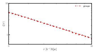
Figure 6: Same as in Figure 5 but for the case of the group auto-correlation function.

Although the linear model at a given scale $r$ depends on the integrals of the real-space angle-averaged correlation function $\xi(r)$ between separation zero and $r$, our measurements of $\xi(r)$ are performed within $\left[0.1,200\right]\,h^{-1}{\rm Mpc}$. We use a power-law form to extrapolate $\xi(r)$ on scales below $0.1\,h^{-1}{\rm Mpc}$.

$$\xi(r<0.1h^{-1}\text{Mpc})=\left(\frac{r}{r_{0}}\right)^{-\gamma}$$ (36)

The power-law parameters $(r_{0},\gamma)$ are measured by fitting $\xi(r)$ on very small scales, i.e. $[0.1,0.25]\,h^{-1}{\rm Mpc}$ in the case of the galaxy auto-correlation and the group-galaxy cross-correlation functions. For the group auto-correlation, given the low clustering due to the low number pairs of group-sized dark matter haloes on scales below $\sim 1\text{-}2h^{-1}$ Mpc, we extrapolate $\xi_{\rm gr}(r)$ on scales below $3h^{-1}\text{Mpc}$ and the power-law parameters are obtained fitting the measured $\xi_{\rm gr}$ in $\left[3,10\right]h^{-1}\text{Mpc}$. The fitting results are listed in Table 1 and shown in Figure 5 for the cross-correlation (green line) and the galaxy auto-correlation(blue line) and in Figure 6 for the group auto-correlation (red line). In Figures 5 and 6, the error bars related to the statistical errors on the measured correlation functions are smaller than the size of the plot symbols.

	$r_{0}$ [$\,h^{-1}{\rm Mpc}$]	$\gamma$
Galaxy auto-correlation	$8.9^{+0.7}_{-0.6}$	$1.75^{+0.03}_{-0.03}$
Group auto-correlation	$8.59^{+0.02}_{-0.02}$	$1.589^{+0.006}_{-0.006}$
Group-galaxy cross-correlation	$5.6^{+0.3}_{-0.3}$	$2.21^{+0.03}_{-0.03}$

Table 1: Power-law $\xi(r)=(r/r_{0})^{-\gamma}$ parameters estimated fitting the real-space two-point auto-correlation function of galaxies and the group-galaxy cross-correlation function, averaged over 27 equal sub-samples, between $[0.1,0.25]\,h^{-1}{\rm Mpc}$. The same parameters in the case of the group auto-correlation function are estimated fitting it between $[3,10]\,h^{-1}{\rm Mpc}$.

3.4.3 $\xi(r)$ Integrals

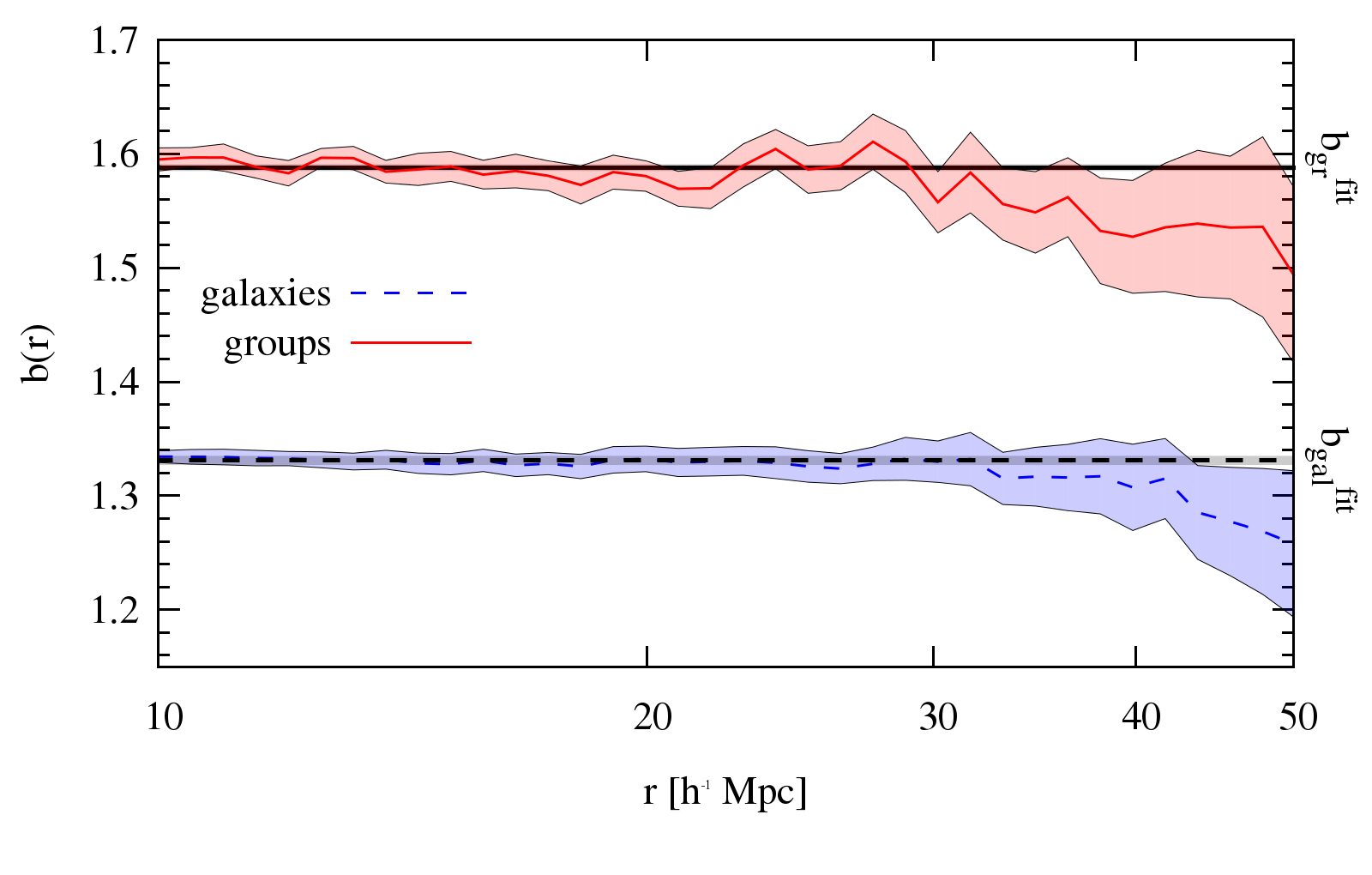
Figure 7: Measurements of the galaxy linear bias $b_{\rm gal}(r)$ and related $1\text{-}\sigma$ errors are shown with blue dashed line and filled blue contours. The red continuous line with red filled contours represent the measurement of the groups linear bias $b_{\rm gr}(r)$ and its $1\text{-}\sigma$ statistical errors. The black dashed and continuous lines with grey contours represent the best fit of data, respectively for the galaxy and groups linear bias factor, between $\left[10,50\right]\,h^{-1}{\rm Mpc}$ with a constant model $b^{mod}=\text{const}$.

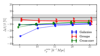
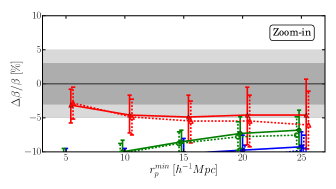
Figure 8: Systematic errors on the galaxy distortion parameter $\beta_{\rm gal}$ estimated by fitting the anisotropic (HOD, $L>1L*$) galaxy auto-correlation function (blue lines) and the group-galaxy cross-correlation function (green lines) and on the group distortion parameter $\beta_{\rm gr}$ from the anisotropic ($M>10^{13}h^{-1}M_{\odot}$ dark matter haloes) group auto-correlation function (red lines), using only the diagonal elements of the covariance matrix, are plotted. The continuous lines with filled points represent results using the Dispersion model. The dashed lines with empty points correspond to fits using the linear Kaiser/Hamilton model only. The error bars correspond to the scatter among the 27 sub-samples used in each analysis. The right panel is just a zoom of the left panel. The shaded regions represent the $5\%$ and $10\%$ levels in the left panel while in the right panel are shifted to $3\%$ and $5\%$ level.

Here we compute the integrals of the real-space angle-averaged correlation functions $\xi(r)$ defined in equations (20a) and (20b). The integration is performed by splitting it into two parts:

$$\bar{\xi}(r)=\frac{3}{r^{3}}\left\{\frac{r_{0}^{\gamma}}{3-\gamma}r_{\rm pl}^{3-\gamma}+\int_{r_{\rm pl}}^{r}r^{\prime 2}\xi(r)dr^{\prime}\right\}$$ (37a)

$$\bar{\bar{\xi}}(r)=\frac{5}{r^{5}}\left\{\frac{r_{0}^{\gamma}}{5-\gamma}r_{\rm pl}^{5-\gamma}+\int_{r_{\rm pl}}^{r}r^{\prime 4}\xi(r)dr^{\prime}\right\}$$ (37b)

Here $r_{\rm pl}$ corresponds to the upper limit of the power-law extrapolation, which is $r_{\rm pl}=0.1h^{-1}\text{Mpc}$ for the galaxy auto-correlation and the group-galaxy cross-correlation and $r_{\rm pl}=3h^{-1}\text{Mpc}$ for the group auto-correlation. In (37a) and (37b) the first terms come from the power-laws on scales between $\left[0,r_{\rm pl}\right]\,h^{-1}{\rm Mpc}$, while the second terms are the integrals of the effective measurements of the real-space 2PCFs.

3.5 Fiducial Model

Among others, one of the advantages in using data from simulations is that we know a priori the expected (i.e. fiducial) values of the quantities we want to measure. This makes them an ideal tool to test and compare the reliability of different methods and theoretical models. In this part we discuss how the fiducial values of the galaxy and group distortion parameters, $\beta_{\rm gal}(z=0.1)$ and $\beta_{\rm gr}(z=0.1)$ have been estimated from the simulated datasets.

To perform this, we need first to estimate the fiducial value for the linear bias $b_{i}$ of our galaxies and groups (haloes). We do this by fitting the quantity

$$b_{i}(r)=\left[\frac{\xi_{i}(r)}{\xi_{\rm mass}(r)}\right]^{1/2}$$ (38)

in equation (38) with a constant between $\left[10,50\right]\,h^{-1}{\rm Mpc}$. This choice for the fitting range is dictated by the need to exclude both small non-linear scales and BAO scales. Not having at our disposal the catalogue of dark matter particles for the MDR1, we have used CAMB to predict the matter correlation function $\xi_{\rm mass}(r)$ at $z=0.1$. The ratio in equation (38) is shown in Figure 7 as measured for the galaxies (blue dashed line and contours) and groups (red continuous line and contours). We obtain the following values:

$$b_{\rm gal}^{\rm fid}(z=0.1)=(1.331\pm 0.004)$$ (39a)

$$b_{\rm gr}^{\rm fid}(z=0.1)=(1.588\pm 0.003)$$ (39b)

The loss of power on scales $>30\,h^{-1}{\rm Mpc}$ is not problematic since, given the statistical error bars, it is still consistent with the assumption of a constant bias factor.

Once the two values of the linear bias $b_{\rm gal}$ and $b_{\rm gr}$ are measured, the estimation of the relative bias $b_{12}$ is straightforward using eq. (23) and results in:

$$b_{12}(z=0.1)=(0.838\pm 0.003)$$ (40)

Given the cosmology of the MDR1 simulation, we obtain a fiducial value $f^{\rm fid}(z=0.1)=0.5434$, corresponding to the following values for the distortion parameters $\beta_{\rm gal}$ and $\beta_{\rm gr}$:

$$\beta_{\rm gal}^{\rm fid}(z=0.1)=(0.4083\pm 0.0006)$$ (41a)

$$\beta_{\rm gr}^{\rm fid}(z=0.1)=(0.3422\pm 0.0006)$$ (41b)

4 Results

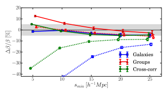
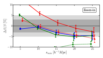
Figure 9: Same as in Figure 8 but now fitting monopole and quadrupole moments of the two-point correlation function in redshift space. Continuous and dashed lines correspond respectively to the dispersion and pure linear models. Note how the linear model fails whenever galaxies are involved using either their auto-correlation or the group-galaxy cross-correlation, while it produces a meaningful result when applied to groups.

We now present the results obtained by fitting the measured two-point correlation functions with the models presented in Section 2. We shall first fit the full $\xi^{s}(r_{p},\pi)$, its multipoles $\xi^{s,(\ell)}(s)$ and the related truncated multipoles $\hat{\xi}^{s,(\ell)}(s)$ using only the diagonal elements of the data covariance matrices; we then perform a full covariance analysis using the truncated multipoles $\hat{\xi}^{s,(\ell)}(s)$.

Several fits are performed, varying the minimum fitting scale in order to study the impact of non-linearities on the accuracy of the measurements as a function of scale. In all cases the maximum scale in the fitting process is limited to a given $s_{\rm max}$, to avoid the complication of modelling the BAO signature.

In the case of fitting the linear Kaiser/Hamilton model, there is only a single free parameter, $\beta$. For the Dispersion model, we must also deal with a nuisance parameter in the form of the pairwise dispersion, $\sigma_{12}$. The constraints on $\beta$ that result from this model are marginalized by integrating the likelihood over a range of $\sigma_{12}$, assuming a uniform prior within a maximum of $\sigma_{12}=10\,h^{-1}{\rm Mpc}$. To some extent, there is a degeneracy between this parameter and $\beta$: raising $\beta$ flattens the contours of $\xi$, whereas the Fingers of God oppose this tendency. But in practice this degeneracy is not severe, reflected in the fact that the errors on $\beta$ are not much greater for the Dispersion model than for the linear model. The significance of treating Fingers of God is therefore more in helping to reduce bias in the best-fitting value of $\beta$.

4.1 Fits to the full anisotropic correlation function

We show here the results of fitting the full $\xi^{s}(r_{p},\pi)$. Fits are performed varying the minimum transverse scale $r_{p}^{\rm min}$, and with a maximum scale fixed at $r_{p}^{\rm max}=\pi^{\rm max}=50\,h^{-1}{\rm Mpc}$. We maximize the likelihood function defined in equation (35), restricted to the diagonal elements of the covariance matrix. Following previous work Hawkins et al. (2003), Guzzo et al. (2008), Bianchi et al. (2012) we fit the quantity

$$y(r_{p},\pi)=\ln\left[1+\xi^{s}(r_{p},\pi)\right]$$ (42)

rather than directly the values of $\xi^{s}(r_{p},\pi)$, in order to enhance the weight of large, more linear scales.

The results for the galaxy auto-correlation (blue lines), group-galaxy cross-correlation (green lines) and the group auto-correlation (red lines) are presented in Figure 8 and the related statistical errors are shown with the error bars. Continuous lines with filled points correspond to fits performed using the Dispersion model while the dashed lines show the results when using the pure linear Kaiser/Hamilton model.

When using the Dispersion model, the galaxy auto-correlation approach underestimates $\beta_{\rm gal}$ by $\sim 10\%$, while the group-galaxy cross-correlation gives similar results when including scales below $10h^{-1}\text{Mpc}$. The recovered values of $\beta_{\rm gal}$ from these two approaches are compatible with each other. On the other hand, the group auto-correlation results yield a much more accurate estimate of the group distortion parameter $\beta_{\rm gr}$, underestimating it by $2\text{-}4\%$. As expected, given the different size of the data sets in these different cases, the statistical errors increase passing from the galaxy auto-correlation to the group-galaxy cross-correlation to the group auto-correlation. Results from the auto-correlations of galaxies and groups are in full agreement with the previous work of Okumura & Jing (2011), de la Torre & Guzzo (2012) and Bianchi et al. (2012). In particular, Figure 5 in the last of these papers shows how the classical approach underestimates $\beta$ by $\sim 10\%$ for the case of haloes with mass $\sim 10^{12}M_{\odot}$ and that this systematic error diminishes for increasing halo masses, being close to unbiased for $\sim 10^{13}M_{\odot}$ i.e. for group-sized haloes.

On scales below $15\,h^{-1}{\rm Mpc}$, the pure linear model heavily underestimates the distortion parameter with respect to the dispersion model when applied to the galaxy auto-correlation. Such discrepancy decreases using first the group-galaxy cross-correlation and disappears almost completely in the case of the group auto-correlation. This shows how the corrections to the linear model on intermediate quasi-linear scales, made through the dispersion model, become gradually less important using objects less affected by the non-linear effects on such scales.

The results from the analysis in this section match our initial expectations. Specifically, using objects tracing higher-mass haloes we are in general less sensitive to the details of non-linear corrections, as previously shown by Bianchi et al. (2012). This is particularly true for the auto-correlation of groups, where we see that the linear and Dispersion models perform similarly even when including small scales. This is at variance with what we observe for galaxies. The use of the cross-correlation, in this case, represents a reasonable compromise between having a larger statistics (thus smaller error bars), while limiting the systematic errors. In the next session, we shall see how a different way of fitting the data can further ameliorate these results, in particular for the cross-correlation function.

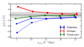
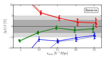
Figure 10: Same as in Figure 8 but now fitting truncated monopole and quadrupole moments of the 2PCF in redshift space.

4.2 Fits to the standard multipole moments

We perform here joint fits of the monopole $\xi^{s,\left(0\right)}\left(s\right)$ and the quadrupole $\xi^{s,\left(2\right)}\left(s\right)$ of the 2PCF in redshift space. We do not consider higher order moments, which are too noisy. To reduce scale dependence, rather than fitting the multipoles directly, we consider the quantity (e.g. de la Torre et al. 2013)

$$y^{s,(\ell)}(s)=s^{2}\,\xi^{s,(\ell)}(s),$$ (43)

which we fit between a varying minimum scale $s_{\rm min}$ and a maximum separation $s_{\rm max}=80\,h^{-1}{\rm Mpc}$. Also in this case we limit the likelihood function in equation (35) to the diagonal elements of the covariance matrix. As in the previous case, we fit using both the full Dispersion model and the simple linear model only, with results plotted as solid and dashed lines, respectively, in Figure 9.

The measurements show a different behaviour, when compared to the fits to the full $\xi^{s}(r_{p},\pi)$. Overall, the results are much more sensitive to the minimum fitting scale $s_{\rm min}$. Also, the linear model gives highly biased results whenever galaxies are involved (either using their auto-correlation or the group-galaxy cross-correlation), producing a meaningful result only when applied to groups alone.

The measurements from the galaxy auto-correlation (blue line) and the group-galaxy cross-correlation (green line) are now very similar, with an overall systematic error on $\beta$, which remains confined to values smaller than $5\%$. On the other hand, the estimates from the group auto-correlation function have a highly scale-dependent behaviour, with a significant positive bias when including scales below 10 $\,h^{-1}{\rm Mpc}$. All approaches converge to a systematic (negative) error of $3-5\%$ when using only scales $>25\,h^{-1}{\rm Mpc}$.

We note how in this case, compared to the analysis using the full $\xi^{s}(r_{p},\pi)$, there is no clear indication that one method performs better than another. We interpret this as the consequence of the projection of the 2PCF onto the Legendre polynomials, which re-distributes over all scales $s$ the non-linear effects originally mostly confined to small transverse scales $r_{p}$. As a consequence, limiting the fitting range to be above a given $s_{\rm min}$ does not eliminate such small-scale contribution.

4.3 Fits to the truncated multipole moments

As described in Section 2.2, we apply now the truncated multipole moments (equation 28). These have been specifically defined as to eliminate the contribution of small transverse scales $r_{p}$, which, as we have just seen, affect all separations $s$. As in the previous section, we perform a joint fit of the quantity in equation (43) for the case of the truncated monopole $\ell=0$ and quadrupole $\ell=2$ using only diagonal errors and for the usual varying ranges in scale.

The results, plotted in Figure 10, show a quite different situation from that of the two previous sections. The estimates using the galaxy auto-correlation function (blue lines) are not improved compared to using the full multipoles, but maintain a typical negative systematic error of $\sim 5\%$. Conversely, the estimates using the group auto-correlation (red lines) show a positive bias for any fitting range, converging to percent errors when including only scales larger than 15 $\,h^{-1}{\rm Mpc}$. Finally, in this case the fits to the cross-correlation are surprisingly stable, almost independently of the fitted range, with an expected systematic error of 3 % or less for $s_{\rm min}>10\,h^{-1}{\rm Mpc}$.

As evident from the dashed lines, using the linear model alone gives in general virtually identical results to the fit using the dispersion model. The only marginal exception is the case of the galaxy auto-correlation. This overall behaviour indicates how the truncated multipoles are able to suppress the weight of small-scale non-linearities, thus making the role of the dispersion factor negligible. In the case of the galaxy auto-correlation, there is still a difference between the two approaches when including scales below $15\,h^{-1}{\rm Mpc}$ in the fit, indicating the stronger effect of non-linearities in this case, compared to when groups are involved. Overall, we can conclude that the newly defined statistic of truncated multipole moments is helpful in reducing the impact of non-linearities on all scales in the measurements.

4.4 Full covariance matrix analysis

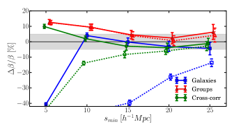
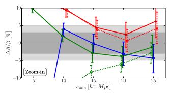
Figure 11: Same as in Figure 9 but now fits are performed using the joint covariance matrix of standard monopole and quadrupole moments of the 2PCF in redshift space.

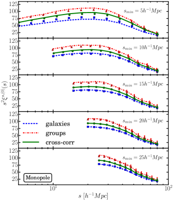
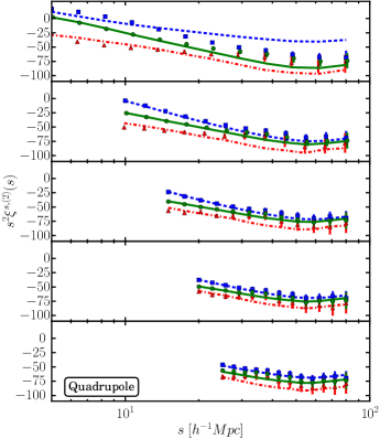
Figure 12: Measurements (points with error-bars) and the related best fit models (lines) for the standard monopole (left panels) and quadrupole (right panels). Blue squares and dashed lines represent the auto-correlation of (HOD, $L>1L*$) galaxies, red triangles and dash-dotted lines represent the auto-correlation of ($M>10^{13}h^{-1}M_{\odot}$ dark matter haloes) groups while their cross-correlation is shown through green circles and continuous lines. Each row shows fit performed using the Dispersion model and full covariance matrix at different minimum fitting scales $s_{min}$.

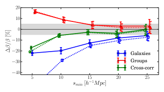
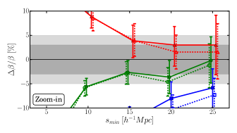
Figure 13: Same as in Figure 10 but now fits are performed using the joint covariance matrix of truncated monopole and quadrupole moments of the PCF in redshift space.

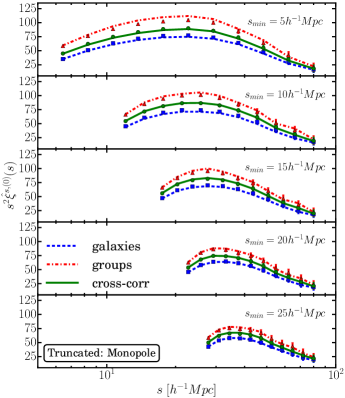
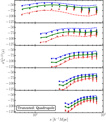
Figure 14: Same as in Figure 12 but for truncated multipole moments.

Measurements of the two-point correlation function in two different bins $i$ and $j$ are, in general, correlated with each other. Keeping in mind that the estimate and use of a proper covariance matrix is a non-trivial issue (see e.g. de la Torre & Guzzo 2012), we explore here the impact of including the full covariance matrix in the analysis of the standard and truncated multipole moments. Specifically, we estimate and use the joint covariance matrix of the truncated monopole $(\ell=0)$ and quadrupole $(\ell=2)$. This means measuring not only the covariance between the measurements of the monopole $y^{s,(0)}(s)$ and quadrupole $y^{s,(2)}(s)$ in two different bins separately but also the cross-covariance between the measurement of the monopole $y^{s,(0)}(s)$ in a given bin $i^{\prime}$ and that of quadrupole $y^{s,(2)}(s)$ in bin $j^{\prime}$. To do this we store the measurements of the monopole $y^{s,(0)}$ and the quadrupole $y^{s,(2)}$, concatenating them into a single array. The covariance matrix is then measured using the definition in equation (34) from 27 sub-sample realizations. We recall that to avoid a singular covariance matrix and keep a good spatial resolution in our measurements we keep fixed the number of bins in the fitting range $[s_{min},80]\,h^{-1}{\rm Mpc}$, independently of $s_{min}$.

We repeat the analysis of standard and truncated multipole moments of the 2PCF but now including the full data covariance matrix in the fitting procedure. The best-fitting models are presented in Figures 12 and 14, and the systematic errors on $\beta$ in Figures 11 and 13. In general, we find the behaviours with minimum fitting scale for the different types of correlation to be similar to the case where only diagonal elements of the covariance matrix are used. The statistical errors on $\beta$ are however larger, as expected, and the detailed dependence on minimum fitting scale slightly noisier, consistently with the increased statistical errors. The only marginal difference in systematics compared to the diagonal covariance case, is in the galaxy auto-correlation where we note that both Kaiser and Dispersion models recover lower values of $\beta$ than previously, in particular for $s_{min}\leq 20\,h^{-1}{\rm Mpc}$. This analysis confirm the results obtained previously and based on using diagonal covariance matrix. It confirms in particular the significantly improved performances of the truncated multipole moments of the galaxy-group cross-correlation with linear Kaiser model.

4.5 Dependence of the results on the mass threshold of the group catalogue

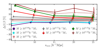
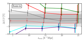
Figure 15: Global dependence of the systematic errors on $\beta$ obtained from the group 2PCF, when the mass threshold of the group catalogue is increased (Table 2). These tests use the truncated multipoles and include the full covariance matrix. As in previous plots, the dashed lines and empty markers in the left plot correspond to using the simple Kaiser model fit. The right panel is a zoom in, including only the Dispersion model curves, to avoid confusion. The red curve ($M>10^{13}h^{-1}M_{\odot}$) corresponds to the group catalogue used so far in the analyses.

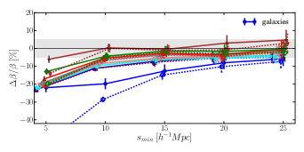
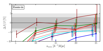
Figure 16: Same as in Figure 15, but now for the cross-correlation of groups and galaxies as defined before. The values obtained from the galaxy 2PCF are also shown as blue squares and lines, for comparison. The colour coding for other curves is the same as in Figure 15.

$\mbox{Log}[M_{min}/(h^{-1}M_{\odot})]$	$N$	$b_{gr}$	$\beta_{gr}^{fid}$	$b_{12}$
$12.00$	$3,439,747$	$1.041\pm 0.001$	$0.5220\pm 0.0005$	$1.279\pm 0.004$
$12.25$	$1,997,835$	$1.133\pm 0.001$	$0.4796\pm 0.0004$	$1.175\pm 0.004$
$12.50$	$1,140,387$	$1.254\pm 0.002$	$0.4333\pm 0.0007$	$1.061\pm 0.004$
$12.75$	$640,598$	$1.402\pm 0.002$	$0.3876\pm 0.0006$	$0.949\pm 0.003$
$13.00$	$350,518$	$1.588\pm 0.003$	$0.3422\pm 0.0006$	$0.838\pm 0.003$
$13.25$	$184,238$	$1.810\pm 0.004$	$0.3002\pm 0.0007$	$0.735\pm 0.003$
$13.50$	$92,403$	$2.094\pm 0.006$	$0.2595\pm 0.0007$	$0.636\pm 0.003$

Table 2: Main parameters for the catalogues of the dark matter haloes used as proxies for galaxy groups in Section 4.5. The first column contains the minimum mass limit for each catalogue, $N$ is the number of objects, $b_{gr}$ is the linear bias, $\beta_{gr}^{fid}$ is the fiducial value for the distortion parameter and $b_{12}$ is the relative bias between galaxies and groups as defined in Equation (23).

So far we have used as “groups” a catalogue of dark matter haloes with $M>10^{13}h^{-1}M_{\odot}$. In this section we test how strong is the dependence of the main results obtained so far, on this mass threshold. To this end, we create the set of group catalogues listed in table 2. We limit our tests to using the truncated multipole moments of the 2PCF and obviously include the full covariance matrix of the data. The results for the group auto correlation are plotted in Figure 15. These show a monotonic trend of the systematic error, almost independently of the minimum fitting scale $s_{min}$. The “sweet spot” for which the error is minimised appears to correspond to masses around $10^{12.50}h^{-1}M_{\odot}$. This behaviour agrees with the previous result obtained by Bianchi et al. (2012) using halo catalogues from the BASICC simulation.

A similar trend is seen in the group-galaxy cross correlation (Figure 16), but in this case there is a dependence on the minimum fitting scale and a general tendency to underestimate the value of the distortion parameter for all group catalogues. From this figure, we see that the group catalogue used for most of the tests in the paper (i.e. $M>10^{13}h^{-1}M_{\odot}$ – green line) is fairly representative of the general behaviour of the cross-correlation function when used to estimate $\beta$.

5 Discussion and Conclusions

This work has explored two different ways of improving the accuracy of the measurement of the growth rate of cosmological structure: by using the cross-correlation of individual galaxies with groups of galaxies as well as by using a novel estimator of the two-point statistics in redshift space, the truncated multipole moments. The aim is to reduce the impact of non-linearities arising from small-scale random peculiar pairwise velocities, with respect to the usual approach of using the multipole moments of the galaxy auto-correlation. We have used a set of simulated catalogues of galaxies to compare the accuracy with which the anisotropic 2PCF $\xi^{s}(r_{p},\pi)$, its multipole moments $\xi^{s,(\ell)}(s)$, and its truncated multipole moments $\smash{\hat{\xi}^{s,(\ell)}(s)}$, allow the recovery of the RSD parameters $\beta$. In this comparison we compared both linear theory and the Dispersion model for RSD.

We find that fitting the full anisotropic auto-correlation function of galaxies underestimates the distortion parameter by about $10\%$, confirming the results of Bianchi et al. (2012). The group-galaxy cross-correlation reduces this bias to a level of about $7\text{-}8\%$, and the group auto-correlation (for groups with mass larger than $10^{13}h^{-1}M_{\odot}$) provides us with even less biased results, reaching an accuracy of about $5\%$. As one may have expected, there is almost no difference between using either linear theory or the Dispersion model when fitting the group auto-correlation function: the Finger of God effect on group centroids is rather minor.

The analysis of standard multipole moments gives no clear indications of the best choice of tracer for RSD. While the galaxy auto-correlation and the group-galaxy cross-correlation lead to similar results, the group auto-correlation produces highly scale-dependent measurements of the distortion parameter. Such complications can mostly be explained by the fact that strong non-linearities on small transverse scales $r_{p}$ are integrated over all scales when projecting the 2PCF on Legendre polynomials, which are not captured by linear or dispersion RSD models. This does not happen when fitting the full $\xi(r_{p},\pi)$ after excluding scales below a given $r_{p}$.

This problem is alleviated by the truncated multipole moments that we have introduced. These provide the most accurate estimates of the distortion parameter among the present tests, improving the accuracy over the use of $\xi^{s}(r_{p},\pi)$ and $\xi^{s,(\ell)}(s)$. In that case, the galaxy auto-correlation underestimates the distortion parameter by about $5\%$, while the group auto-correlation becomes gradually less biased when using larger minimum scales to reach a few percent accuracy on scales greater than $20\,h^{-1}{\rm Mpc}$. The group-galaxy cross-correlation, when similarly fitted with the Dispersion model, produces more stable and also more accurate measurements of $\beta$, reaching the percent level of accuracy when fitting scales greater than $15\,h^{-1}{\rm Mpc}$. A comparison with the results from the linear model shows how the truncated multipole moments allow reducing the impact of small-scale non-linearities in RSD measurements, making possible the analysis with the simple linear model. In fact, for the galaxy auto-correlation, the limit at which the Dispersion model breaks down is translated to $15\,h^{-1}{\rm Mpc}$, compared with $20\,h^{-1}{\rm Mpc}$ in the case of the anisotropic 2PCF.

We studied the impact of bin-to-bin covariances in the fitting procedure and found no significant difference in terms of systematics, confirming our findings based on using only the diagonal covariance matrix.

Finally, we have directly tested how our general results may depend on the mass threshold chosen to define the the group catalogue used for most of the tests ($10^{13}h^{-1}M_{\odot}$). The exercise using a set of further six group catalogues, with minimum mass thresholds ranging from $10^{12}h^{-1}M_{\odot}$ to $10^{13.5}h^{-1}M_{\odot}$, shows that the “standard” group catalogue is fairly representative of the general trend observed in the systematic errors when using the cross correlation function. Additionally, it further confirms the dependence of the errors on the halo mass threshold, evidenced in Bianchi et al. (2012).

Although none of the methods studied here yields a zero bias, we find the results encouraging. Small systematics at the few percent level arise in RSD from other effects to do with the sky sampling (de la Torre et al. 2013), and these are already corrected for by analysis of mock data. The same approach could be taken in order to incorporate small systematic errors in the theoretical RSD models being used, although further work will be required in order to demonstrate that these systematic offsets themselves are consistent independent of the true cosmology under study.

The other element of this study that could benefit from extension concerns the group catalogue. The present work is somewhat idealised in that the group proxies are dark-matter haloes that are found directly in the simulation using more information than would be available in a real galaxy survey. The next step is therefore to repeat this analysis using a full simulation of the construction of an empirical group catalogue by linking the simulated galaxies in redshift space (following e.g. Robotham et al. 2011). At large group masses, uncertainties in group centroids should not be large, and so the features of the present work in terms of small Fingers of God should be reproduced.

References

- Alam et al. (2015) Alam, S., Ho, S., Vargas-Magaña, M., & Schneider, D. P. 2015, MNRAS, 453, 1754
- Beutler et al. (2014) Beutler, F., Saito, S., Seo, H.-J., et al. 2014, MNRAS, 443, 1065
- Bianchi et al. (2012) Bianchi, D., Guzzo, L., Branchini, E., et al. 2012, MNRAS, 427, 2420
- Bianchi et al. (2014) Bianchi, D., Chiesa, M., & Guzzo, L. 2014, arXiv:1407.4753
- Blake et al. (2011) Blake, C., Brough, S., Colless, M., et al. 2011, MNRAS, 415, 2876
- Cabré & Gaztañaga (2009a) Cabré, A., & Gaztañaga, E. 2009, MNRAS, 393, 1183
- Cabré & Gaztañaga (2009b) Cabré, A., & Gaztañaga, E. 2009, MNRAS, 396, 1119
- Carroll et al. (2004) Carroll, S. M., Duvvuri, V., Trodden, M., & Turner, M. S. 2004, Phys.Rev.D, 70, 043528
- Cole et al. (1994) Cole, S., Fisher, K. B., & Weinberg, D. H. 1994, MNRAS, 267, 785
- Contreras et al. (2013) Contreras, C., Blake, C., Poole, G. B., et al. 2013, MNRAS, 683
- de la Torre & Guzzo (2012) de la Torre, S., & Guzzo, L. 2012, MNRAS, 427, 327
- de la Torre et al. (2013) de la Torre, S., Guzzo, L., Peacock, J. A., et al. 2013, A&A, 557, A54
- Elia et al. (2012) Elia, A., Ludlow, A. D., & Porciani, C. 2012, MNRAS, 421, 3472
- Eke et al. (2004) Eke, V. R., Baugh, C. M., Cole, S., et al. 2004, MNRAS, 348, 866
- Fisher et al. (1994) Fisher, K. B., Davis, M., Strauss, M. A., Yahil, A., & Huchra, J. P. 1994, MNRAS, 267, 927
- Guzzo et al. (2008) Guzzo, L., Pierleoni, M., Meneux, B., et al. 2008, Nature, 451, 541
- Hamilton (1992) Hamilton, A. J. S. 1992, ApJL, 385, L5
- Hartlap et al. (2007) Hartlap, J., Simon, P., & Schneider, P. 2007, A&A, 464, 399
- Hawkins et al. (2003) Hawkins, E., Maddox, S., Cole, S., et al. 2003, MNRAS, 346, 78
- Joyce et al. (2014) Joyce A., Jain B., Khoury J., Trodden M., 2014, arXiv, arXiv:1407.0059
- Kaiser (1987) Kaiser, N. 1987, MNRAS, 227, 1
- Landy & Szalay (1993) Landy, S. D., & Szalay, A. S. 1993, ApJ, 412, 64
- Laureijs et al. (2011) Laureijs, R., Amiaux, J., Arduini, S., et al. 2011, arXiv:1110.3193
- Lewis et al. (2000) Lewis, A., Challinor, A., & Lasenby, A. 2000, ApJ, 538, 473
- Mandelbaum et al. (2013) Mandelbaum, R., Slosar, A., Baldauf, T., et al. 2013, MNRAS, 432, 1544
- Merloni et al. (2012) Merloni, A., Predehl, P., Becker, W., et al. 2012, arXiv:1209.3114
- Mountrichas et al. (2009) Mountrichas, G., Sawangwit, U., Shanks, T., et al. 2009, MNRAS, 394, 2050
- Munari et al. (2013) Munari, E., Biviano, A., Borgani, S., Murante, G., & Fabjan, D. 2013, MNRAS, 430, 2638
- Okumura & Jing (2011) Okumura, T., & Jing, Y. P. 2011, ApJ, 726, 5
- Peacock et al. (2001) Peacock, J. A., Cole, S., Norberg, P., et al. 2001, Nature, 410, 169
- Peacock & Dodds (1994) Peacock, J. A., & Dodds, S. J. 1994, MNRAS, 267, 1020
- Percival et al. (2004) Percival, W. J., Burkey, D., Heavens, A., et al. 2004, MNRAS, 353, 1201
- Perlmutter et al. (1999) Perlmutter, S., Aldering, G., Goldhaber, G., et al. 1999, ApJ, 517, 565
- Prada et al. (2012) Prada, F., Klypin, A. A., Cuesta, A. J., Betancort-Rijo, J. E., & Primack, J. 2012, MNRAS, 423, 3018
- Reid & White (2011) Reid, B. A., & White, M. 2011, MNRAS, 417, 1913
- Reid et al. (2014) Reid, B. A., Seo, H.-J., Leauthaud, A., Tinker, J. L., & White, M. 2014, MNRAS, 444, 476
- Riess et al. (1998) Riess, A. G., Filippenko, A. V., Challis, P., et al. 1998, AJ, 116, 1009
- Robotham et al. (2011) Robotham A. S. G., et al., 2011, MNRAS, 416, 2640
- Ross et al. (2007) Ross, N. P., da Ângela, J., Shanks, T., et al. 2007, MNRAS, 381, 573
- Samushia et al. (2014) Samushia, L., Reid, B. A., White, M., et al. 2014, MNRAS, 439, 3504
- Sánchez et al. (2014) Sánchez, A. G., Montesano, F., Kazin, E. A., et al. 2014, MNRAS, 440, 2692
- Scoccimarro (2004) Scoccimarro, R. 2004, Phys.Rev.D, 70, 083007
- Taruya et al. (2010) Taruya, A., Nishimichi, T., & Saito, S. 2010, Phys.Rev.D, 82, 063522
- Tegmark et al. (2004) Tegmark, M., Blanton, M. R., Strauss, M. A., et al. 2004, ApJ, 606, 702
- van den Bosch et al. (2004) van den Bosch, F. C., Norberg, P., Mo, H. J., & Yang, X. 2004, MNRAS, 352, 1302
- Zheng et al. (2005) Zheng, Z., Berlind, A. A., Weinberg, D. H., et al. 2005, ApJ, 633, 791
- Zurek et al. (1994) Zurek, W. H., Quinn, P. J., Salmon, J. K., & Warren, M. S. 1994, ApJ, 431, 559
- Zu & Weinberg (2013) Zu, Y., & Weinberg, D. H. 2013, MNRAS, 431, 3319