Amplification uncertainty relation for probabilistic amplifiers

Abstract

Traditionally, quantum amplification limit refers to the property of inevitable noise addition on canonical variables when the field amplitude of an unknown state is linearly transformed through a quantum channel. Recent theoretical studies have determined amplification limits for cases of probabilistic quantum channels or general quantum operations by specifying a set of input states or a state ensemble. However, it remains open how much excess noise on canonical variables is unavoidable and whether there exists a fundamental trade-off relation between the canonical pair in a general amplification process. In this paper we present an uncertainty-product form of amplification limits for general quantum operations by assuming an input ensemble of Gaussian distributed coherent states. It can be derived as a straightforward consequence of canonical uncertainty relations and retrieves basic properties of the traditional amplification limit. In addition, our amplification limit turns out to give a physical limitation on probabilistic reduction of an Einstein-Podolsky-Rosen uncertainty. In this regard, we find a condition that probabilistic amplifiers can be regarded as local filtering operations to distill entanglement. This condition establishes a clear benchmark to verify an advantage of non-Gaussian operations beyond Gaussian operations with a feasible input set of coherent states and standard homodyne measurements.

I Introduction

It is fundamental to ask how an amplification of canonical variables modifies the phase-space distribution of amplified states under the physical constraint due to canonical uncertainty relations. The standard theory to address this question is the so-called amplification uncertainty principle amp . It describes the property of inevitable noise addition on canonical variables when the field amplitude of an unknown state is linearly transformed through a quantum channel. This traditional form of quantum amplification limits is directly derived from the property of canonical variables, and gives an important insight on a wide class of experiments in quantum optics, quantum information science YY86 ; Cerf00 ; Cerf00R ; Lind00 ; Andersen05 ; rmp-clone ; Josse06 ; Koike06 ; Sab07 ; Pooser09 ; Weed12 , and condensed matter physics Cle10 . Unfortunately, the linearity of amplification maps assumed in this theory is hardly satisfied in the experiments ComLR , although this assumption corresponds to a covariance property that works as an essential theoretical tool to analyze a general property of amplification and related cloning maps Gut06 ; Cer05 . It is more realistic to consider the performance of amplifiers in a limited input space. In fact, one can find a practical limitation by focusing on a set of input states or an ensemble of input states Namiki11R ; Chir13 ; Pande13 .

There has been a growing interest in implementing probabilistic amplifiers in order to overcome the standard limitation of the traditional amplification limit Ralph09 ; Ferreyrol2010 ; Usuga2010 ; Xiang2010a ; Zavatta2011 ; Chrzanowski2014 . In these approaches, one can obtain essentially noiselessly amplified coherent states with a certain probability by conditionally choosing the output of the process. Recent theoretical studies have determined amplification limits for such cases of probabilistic quantum channels or general quantum operations Chir13 ; Pande13 . Certainly, these results can reach beyond the coverage of the traditional theory. However, it seems difficult to find a precise interrelation between these theories. For example, it is not clear whether the traditional form can be reproduced as a special case of the general theory. At this stage, we may no longer expect an essential role of canonical uncertainty relations in determining a general form of amplification limits.

Another topical aspect on the probabilistic amplification is its connection to entanglement distillation. On the one hand, the no-go theorem of Gaussian entanglement distillation tells us that Gaussian operations are unusable for distillation of Gaussian entanglement Fiurasek ; Giedke2002 . On the other hand, it has been shown that a specific design of non-deterministic linear amplifier (NLA) can enhance entanglement Ralph09 , and experimental demonstrations of entanglement distillation have been reported in Chrzanowski2014 ; Xiang2010a . Thereby, such an enhancement of entanglement could signify a clear advantage of no-Gaussian operations over the Gaussian operations. Interestingly, a substantial difference between an optimal amplification fidelity for deterministic quantum gates and that for probabilistic physical processes has been shown in Ref. Chir13 . In there, a standard Gaussian amplifier is identified as an optimal deterministic process for maximizing the fidelity, while the NLA turns out to achieve the maximal fidelity for probabilistic gates in an asymptotical manner. However, these amplification fidelities have not been associated with the context of entanglement distillation. Hence, it is interesting if one can find a legitimate amplification limit for Gaussian operations such that the physical process beyond the limit demonstrates the advantage of non-Gaussian operations. More fundamentally, we may ask whether an amplification limit for Gaussian operations could be derived as a consequence of the no-go theorem.

The fidelity-based amplification limit Namiki11R ; Chir13 is defined on an input-state ensemble called the Gaussian distributed coherent states. This ensemble has been utilized to demonstrate a non-classical performance of continuous-variable (CV) quantum teleportation Furusawa98 and quantum memories julsgaard04a . The main idea underlying this ensemble is to consider an effectively uniform set of input states in a CV space by using a Gaussian prior. We can sample coherent states with modest input power around the origin of the phase-space with a relatively flat prior while a rapid decay of the prior enables us to suppress the contribution of impractically high-energy input states. Given this ensemble, an experimental success criterion for CV gates is to surpass the classical limit fidelity due to entanglement breaking (EB) maps Horo03a . The classical fidelity was determined for unit-gain channels in Ref. Ham05 and for lossy/amplification channels in Ref. namiki07 (See also Ref. Namiki11 ). Further, the framework was generalized to include whole completely-positive (CP) maps, i.e., general quantum operations Chir13 .

Recently, a different form of such classical limits has been derived using an uncertainty product of canonical variables Namiki-Azuma13x . It gives an optimal trade-off relation between canonical noises in order to outperform EB maps for general amplification/attenuation tasks. This suggests that, instead of the fidelity, one can use an uncertainty product of canonical variables to evaluate the performance of amplifiers. However, for a general amplification process, it remains open (i) how much excess noise is unavoidable on canonical variables and (ii) whether there exists a simple trade-off relation between noises of the canonical pair.

In this paper we resolve above questions by presenting an uncertainty-product form of amplification limits for general quantum operations based on the input ensemble of Gaussian distributed coherent states. It is directly derived by using canonical uncertainty relations and retrieves basic property of the traditional amplification limit. We investigate attainability of our amplification limit and identify a parameter regime where Gaussian channels cannot achieve our bound but the NLA asymptotically achieves our bound. We also point out the role of probabilistic amplifiers for entanglement distillation. Using the no-go theorem for Gaussian entanglement distillation we find a condition that a probabilistic amplifier can be regarded as a local filtering operation to demonstrate entanglement distillation. This condition establishes a clear benchmark to verify an advantage of non-Gaussian operations beyond Gaussian operations with a feasible input set of coherent states and standard homodyne measurements.

The rest of this paper is organized as follows. In section II, we present our amplification limit which is regarded as an extension of the traditional amplification limit amp for two different directions: (i) It determines the limitation with an input ensemble of a bounded power; (ii) It is applicable to stochastic quantum processes as well as quantum channels. In section III, we consider attainability of our amplification limit for Gaussian and non-Gaussian amplifiers. In section IV, we address the connection between our amplification limit and entanglement distillation. We conclude this paper with remarks in section V.

II general amplification limits for Gaussian distributed coherent states

In this section we present a general amplification limit for Gaussian distributed coherent states which is applicable to either probabilistic or deterministic quantum process. We review the fidelity-based results of amplification limits in subsection II.1 partly as an introduction of basic notations. We present our main theorem in subsection II.2.

II.1 Fidelity-based amplification limits

We consider transmission of coherent states $\{\left|\alpha\right\rangle\}_{\alpha\in\mathbb{C}}$ drawn from a Gaussian prior distribution with an inverse width $\lambda>0,$

$$p_{\lambda}(\alpha):=\frac{\lambda}{\pi}\exp(-\lambda|\alpha|^{2}).$$ (1)

We call the state ensemble $\{p_{\lambda}(\alpha),\left|\alpha\right\rangle\}_{\alpha\in{\mathbb{C}}}$ the Gaussian distributed coherent states. A main motivation to use the Gaussian prior of Eq. (1) is to execute a uniform sampling of the input amplitude around the origin of the phase-space $|\alpha|^{2}\ll\lambda^{-1}$ with keeping out the contribution of higher power input states for $|\alpha|^{2}>\lambda^{-1}$ by properly choosing the inverse width $\lambda>0$. A uniform average over the phase-space or an ensemble of completely unknown coherent states can be formally described by taking the limit $\lambda\to 0$.

Let us refer to the following state transformation as the phase-insensitive amplification/attenuation task of a gain $\eta\geq 0$,

$$\left|\alpha\right\rangle\to\left|\sqrt{\eta}\alpha\right\rangle.$$ (2)

We say the task is an amplification (attenuation) if $\eta\geq 1$ ($\eta<1$). We may specifically call the task of $\eta=1$ the unit gain task. We define an average fidelity of the phase-insensitive task for a physical map $\mathcal{E}$ as

$$F_{\eta,\lambda}:={\int p_{\lambda}(\alpha)\left\langle\sqrt{\eta}\alpha\right|\mathcal{E}(\rho_{\alpha})\left|\sqrt{\eta}\alpha\right\rangle d^{2}\alpha}.$$ (3)

Note that we use the following notation for the density operator of a coherent state throughout this paper:

$$\rho_{\alpha}=\left|\alpha\right\rangle\left\langle\alpha\right|.$$ (4)

The fidelity-based amplification limit Namiki11R ; Chir13 is given as follows: For any quantum operation $\mathcal{E}$, i.e., a CP trace-non-increasing map, it holds that

$$F_{\eta,\lambda}^{({\rm Prob})}:=\frac{F_{\eta,\lambda}}{P_{s}}\leq\frac{1}{2}\left(\frac{1+\lambda}{\eta}+1+\left|\frac{1+\lambda}{\eta}-1\right|\right),$$ (5)

where $P_{s}$ is the probability that $\mathcal{E}$ gives an output state for the ensemble $\{p_{\lambda}(\alpha),\rho_{\alpha}\}$. It is defined as

$$P_{s}:={{\textrm{Tr}}\int p_{\lambda}(\alpha)\mathcal{E}(\rho_{\alpha})d^{2}\alpha}.$$ (6)

As we will see in the next subsection, this probability represents a normalization factor when $\mathcal{E}$ acts on a subsystem of a two-mode squeezed state. Note that $P_{s}=1$ if $\mathcal{E}$ is a quantum channel, i.e., a CP trace-preserving map.

In analogous to Eq. (2), we may define a symmetric phase-conjugation task associated with the state transformation:

$$\left|\alpha\right\rangle\to\left|\sqrt{\eta}\alpha^{*}\right\rangle.$$ (7)

Thereby, we may define an average fidelity of this task as

$$F_{\eta,\lambda}^{*}:={\int p_{\lambda}(\alpha)\left\langle\sqrt{\eta}\alpha^{*}\right|\mathcal{E}(\rho_{\alpha})\left|\sqrt{\eta}\alpha^{*}\right\rangle d^{2}\alpha}.$$ (8)

The fidelity-based phase-conjugation limit is given by Namiki11R ; Yang14

$${F_{\eta,\lambda}^{*}}^{({\rm Prob})}=\frac{{F_{\eta,\lambda}^{*}}}{P_{s}}\leq\frac{1+\lambda}{1+\eta+\lambda},$$ (9)

Note that one can generalize the fidelity-based quantum limits in Eqs. (5) and (9) for phase-sensitive cases by introducing modified tasks as

$$\left|\alpha\right\rangle\to S\left|\sqrt{\eta}\alpha\right\rangle,{\rm or\ }\left|\alpha\right\rangle\to S\left|\sqrt{\eta}\alpha^{*}\right\rangle,$$ (10)

where

$$S:=S(r)=e^{r(\hat{a}^{2}-\hat{a}^{\dagger 2})/2}$$ (11)

is a squeezing unitary operation and $r$ represents the degree of squeezing. The quantum limited fidelity values of Eqs. (5) and (9) are invariant under the addition of unitary operators since the optimal map can absorb the effect of additional unitary operators namiki07 ; Namiki12R ; Namiki-Azuma13x .

II.2 Amplification limits via an uncertainty-product of canonical quadrature variables

We may consider a general phase-sensitive amplification/attenuation task in terms of phase-space quadratures so that average quadratures of the input coherent state $\rho_{\alpha}$ of Eq. (4) are transformed as

$$(x_{\alpha},p_{\alpha})\to(\sqrt{\eta_{x}}x_{\alpha},\sqrt{\eta_{p}}p_{\alpha}),$$ (12)

where the gain pair of the amplification/attenuation task $(\eta_{x},\eta_{p})$ is a pair of non-negative numbers, and the mean quadratures for the coherent state $\rho_{\alpha}$ are defined as

$$x_{\alpha}:={\textrm{Tr}}(\hat{x}\rho_{\alpha})=\frac{\alpha+\alpha^{*}}{\sqrt{2}},\ p_{\alpha}:={\textrm{Tr}}(\hat{p}\rho_{\alpha})=\frac{\alpha-\alpha^{*}}{\sqrt{2}i}.$$ (13)

Throughout this paper we assume the canonical commutation relation for canonical quadrature variables $[\hat{x},\hat{p}]=i$, which is consistent with the standard relations such as $\hat{x}=(\hat{a}+\hat{a}^{\dagger})/\sqrt{2}$, $\hat{p}=(\hat{a}-\hat{a}^{\dagger})/(i\sqrt{2})$, and $\hat{a}\left|\alpha\right\rangle=\alpha\left|\alpha\right\rangle$. Similarly to Eq. (12), we may consider a general phase-conjugation task associated with the following transformation:

$$(x_{\alpha},p_{\alpha})\to(\sqrt{\eta_{x}}x_{\alpha},-\sqrt{\eta_{p}}p_{\alpha}).$$ (14)

Given the task of Eq. (12), we may measure the performance of an amplifier $\mathcal{E}$ by using the square deviation,

$${\textrm{Tr}}[(\hat{z}-\sqrt{\eta}_{z}z_{\alpha})^{2}\mathcal{E}(\rho_{\alpha})],$$ (15)

where $z\in\{x,p\}$. Note that, if the mean output quadratures are equal to the output of the transformation of Eq. (12) as ${\textrm{Tr}}[\hat{z}\mathcal{E}(\rho_{\alpha})]=\sqrt{\eta}_{z}z_{\alpha}$, the expression of Eq. (15) turns to the variance of the output quadrature

$${\textrm{Tr}}[(\hat{z}-\sqrt{\eta}_{z}z_{\alpha})^{2}\mathcal{E}(\rho_{\alpha})] ={\textrm{Tr}}[\hat{z}^{2}\mathcal{E}(\rho_{\alpha})]-({\textrm{Tr}}[\hat{z}\mathcal{E}(\rho_{\alpha})])^{2}$$

$$=\langle\Delta^{2}\hat{z}\rangle_{\mathcal{E}(\rho_{\alpha})}.$$ (16)

However, it is impractical to consider that the linearity of the transformation

$${\textrm{Tr}}[\hat{z}\mathcal{E}(\rho_{\alpha})]=\sqrt{\eta}_{z}z_{\alpha}$$ (17)

holds in experiments for every input amplitude $\alpha\in\mathbb{C}$. We thus proceed our formulation without using this condition.

Instead of the point-wise constraint on $\alpha$, we consider an average of the quadrature deviations with the Gaussian prior distribution $p_{\lambda}$ of Eq. (1). We seek for the physical process that minimizes the mean square deviations (MSD) of canonical quadratures: Namiki-Azuma13x

$$\bar{V}_{x}(\eta,\lambda) := {\textrm{Tr}}\int p_{\lambda}(\alpha)(\hat{x}-\sqrt{\eta}x_{\alpha})^{2}\mathcal{E}(\rho_{\alpha})d^{2}\alpha,$$

$$\bar{V}_{p}(\eta,\lambda) := {\textrm{Tr}}\int p_{\lambda}(\alpha)(\hat{p}\mp\sqrt{\eta}p_{\alpha})^{2}\mathcal{E}(\rho_{\alpha})d^{2}\alpha,$$ (18)

where the lower sign of the second expression is for the case of the phase-conjugation task in Eq. (14). The MSDs of Eq. (18) can be observed experimentally by measuring the first and the second moments of the quadratures $\{\hat{x},\hat{p},\hat{x}^{2},\hat{p}^{2}\}$ for the output of the physical process $\mathcal{E}(\rho_{\alpha})$. Due to canonical uncertainty relations, $\bar{V}_{x}$ and $\bar{V}_{p}$ could not be arbitrary small, simultaneously. We can find a rigorous trade-off relation between $\bar{V}_{x}$ and $\bar{V}_{p}$ from the following theorem.

Theorem 1.— For any given $\eta_{x}>0$, $\eta_{p}>0$, and $\lambda>0$, any quantum operation (or stochastic quantum channel) $\mathcal{E}$ satisfies

$$\prod_{z=x,p}\left[\frac{\bar{V}_{z}(\eta_{z},\lambda)}{P_{s}}-\frac{\eta_{z}}{2(1+\lambda)}\right]\geq\frac{1}{4}\left|\frac{\sqrt{\eta_{x}\eta_{p}}}{1+\lambda}\mp 1\right|^{2}$$ (19)

where $P_{s}$ and $\bar{V}_{z}$ are defined in Eqs. (6) and (18), respectively. Moreover, the lower signs of Eqs. (18) and (19) correspond to the case of the phase-conjugation task in Eq. (14).

Proof.—Let $J=J_{AB}$ be a density operator of a two-mode system $AB$ described by $[\hat{x}_{A},\hat{p}_{A}]=[\hat{x}_{B},\hat{p}_{B}]=i$. Canonical uncertainty relations and property of variances lead to

$${\textrm{Tr}}[(\hat{x}_{A}-g_{x}\hat{x}_{B})^{2}J]{\textrm{Tr}}[(\hat{p}_{A}+g_{p}\hat{p}_{B})^{2}J]$$

$$\geq \langle\Delta^{2}(\hat{x}_{A}-g_{x}\hat{x}_{B})\rangle_{J}\langle\Delta^{2}(\hat{p}_{A}+g_{p}\hat{p}_{B})\rangle_{J}\geq\frac{1}{4}(1-g_{x}g_{p})^{2}.$$

Here, we will prove the case of the normal amplification/attenuation process by assuming $g_{x}\geq 0$ and $g_{p}\geq 0$. The proof for the phase-conjugation process runs similarly by considering the case of $g_{x}\geq 0$ and $g_{p}<0$.

From a standard notation $\hat{x}_{B}={(\hat{b}+\hat{b}^{\dagger})}/{\sqrt{2}}$ and the cyclic property of the trace we can write

$${\textrm{Tr}}[(\hat{x}_{A}-g_{x}\hat{x}_{B})^{2}J]$$ (21)

$$= {\textrm{Tr}}[\hat{x}_{A}^{2}{J}-2g_{x}\hat{x}_{A}\left(\frac{\hat{b}^{\dagger}{J}+{J}\hat{b}}{\sqrt{2}}\right)$$

$$+\frac{{g_{x}}^{2}}{2}(\hat{b}^{\dagger 2}{J}+{J}\hat{b}^{2}+2\hat{b}^{\dagger}{J}\hat{b}-J)]$$

$$= {\textrm{Tr}}_{A}\int\frac{d^{2}\alpha}{\pi}(\hat{x}_{A}-g_{x}x_{\alpha})^{2}\left\langle\alpha^{*}\right|J\left|\alpha^{*}\right\rangle_{B}-\frac{g_{x}^{2}}{2},$$

where, in the final line, we execute the partial trace by ${\textrm{Tr}}_{B}[\ \cdot\ ]\to\int\left\langle\alpha^{*}\right|\cdot\left|\alpha^{*}\right\rangle_{B}\frac{d^{2}\alpha}{\pi}$ and use the property of the coherent state $\hat{b}\left|\alpha^{*}\right\rangle_{B}=\alpha^{*}\left|\alpha^{*}\right\rangle_{B}$ and $\left\langle\alpha^{*}\right|_{B}\hat{b}^{\dagger}=\alpha\left\langle\alpha^{*}\right|_{B}$. Similarly, starting from $\hat{p}_{B}=i{(\hat{b}^{\dagger}-\hat{b})}/{\sqrt{2}}$ we have

$${\textrm{Tr}}[(\hat{p}_{A}+g_{p}\hat{p}_{B})^{2}J]$$ (22)

$$= {\textrm{Tr}}_{A}\int\frac{d^{2}\alpha}{\pi}(\hat{p}_{A}-g_{p}p_{\alpha})^{2}\left\langle\alpha^{*}\right|J\left|\alpha^{*}\right\rangle_{B}-\frac{g_{p}^{2}}{2}.$$

Next, suppose that $J$ is prepared by an action of a quantum operation $\mathcal{E}$ as $J=\mathcal{E}_{A}\otimes I_{B}(\left|\psi_{\xi}\right\rangle\left\langle\psi_{\xi}\right|)/P_{s}$ where $\left|\psi_{\xi}\right\rangle=\sqrt{1-\xi^{2}}\sum_{n=0}^{\infty}\xi^{n}\left|n\right\rangle\left|n\right\rangle$ is a two-mode squeezed state with $\xi\in(0,1)$ and $P_{s}:={\textrm{Tr}}[\mathcal{E}_{A}\otimes I_{B}(\left|\psi_{\xi}\right\rangle\left\langle\psi_{\xi}\right|)]$. This implies $\left\langle\alpha^{*}\right|J\left|\alpha^{*}\right\rangle_{B}=(1-\xi^{2})e^{-(1-\xi^{2})|\alpha|^{2}}\mathcal{E}_{A}(\rho_{\xi\alpha})/P_{s}$. From this relation and Eqs. (1), (21), and (22) we obtain

$${\textrm{Tr}}[(\hat{p}_{A}+g_{p}\hat{p}_{B})^{2}J]{\textrm{Tr}}[(\hat{x}_{A}-g_{x}\hat{x}_{B})^{2}J]$$

$$= \prod_{z=x,p}\left({\textrm{Tr}}_{A}\int\frac{d^{2}\alpha}{\pi}(\hat{z}_{A}-g_{z}z_{\alpha})^{2}\left\langle\alpha^{*}\right|J\left|\alpha^{*}\right\rangle_{B}-\frac{g_{z}^{2}}{2}\right)$$

$$= \prod_{z=x,p}\left[\frac{{\textrm{Tr}}\int p_{\lambda}(\alpha)(\hat{z}-\sqrt{\eta}_{z}z_{\alpha})^{2}\mathcal{E}(\rho_{\alpha}){d^{2}\alpha}}{{\textrm{Tr}}\int p_{\lambda}(\alpha)\mathcal{E}(\rho_{\alpha}){d^{2}\alpha}}-\frac{\eta_{z}}{2(1+\lambda)}\right],$$

where, in the final step, we drop the subscript $A$, rescale the integration variable as $\xi\alpha\to\alpha$, and introduce

$$\eta_{x}=(1+\lambda)g_{x}^{2},\ \eta_{p}=(1+\lambda)g_{p}^{2},\ \lambda=\frac{1-\xi^{2}}{\xi^{2}}.$$ (24)

Finally, concatenating Eqs. (18), (LABEL:usr1), (LABEL:LHS), and (24), we can reach our theorem 1 of Eq. (19). $\blacksquare$

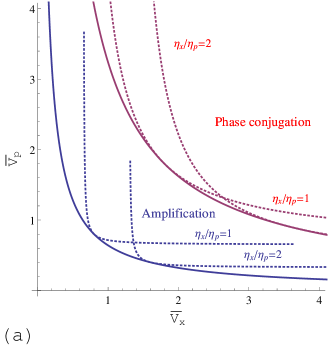
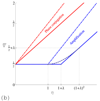
Figure 1: (Color Online) (a) Solid curves represent general lower bounds on the product of the mean square deviations (MSD) of Eq. (18) given by $\bar{V}_{x}\bar{V}_{p}\geq(\eta^{\prime}+|\eta^{\prime}\mp 1|)^{2}/4$ [See Eq. (26)]. Here, an effective gain factor is set to be $\eta^{\prime}={\eta}/({1+\lambda})=1.3$ with the constraint on the gain pair $\sqrt{\eta_{x}\eta_{p}}=\eta$. This constraint parameterizes the gain pair as $(\eta_{x},\eta_{p})=(\eta e^{R},\eta e^{-R})$ with $R\in\mathbb{R}$. The upper solid curve is for the phase-conjugation task and the lower solid curve is for the normal amplification task. Each of them can be determined by taking the intersection of our amplification limits in Eq. (19) with various ratios between the gain pair $\eta_{x}/\eta_{p}=e^{2R}$. Dotted curves represent the cases for $\eta_{x}/\eta_{p}=1$ and $\eta_{x}/\eta_{p}=2$. (b) Typical behavior of the MSDs in the cases of $\bar{V}_{x}=\bar{V}_{p}=\bar{V}$ as a function of the gain $\eta$. The upper solid line represents the limitation on the phase-conjugation process [Eq. (30)] and the lower kinked solid line represents the limitation on the normal amplification/attenuation process [Eq. (28)]. The dashed curve for $\eta\in[1,(1+\eta)^{2}]$ shows the minimum of the MSD due to Gaussian channels $\bar{V}^{\star}$ [Eq. (33)]. Dash-dot lines are due to the traditional form of amplification limits for completely unknown coherent states [Eqs. (69) and (70) with $G=\eta$]. They can be retrieved by our bounds in the limit of $\lambda\to 0$. In this figure we set $\lambda=0.4$ so that the structure around $\eta=1+\lambda$ is displayed clearly. When $\eta=0$, all lines indicate the minimum value of $\bar{V}=1/2$ due to canonical uncertainty relations as it corresponds to the trivial case of $g_{x}=g_{p}=0$ in Eq. (LABEL:usr1).

Our theorem 1 states that any physical map is unable to break the uncertainty-relation-type trade-off inequality for quadrature deviations on average. It draws an inverse-proportional curve in the $\bar{V}_{x}$-$\bar{V}_{p}$ plane with a given pair of $(\eta_{x},\eta_{p})$, and the area below the curve is unattainable by any quantum process including probabilistic amplifiers [See FIG. 1(a)]. Equation (19) is essentially the same structure as the traditional form of amplification limits amp [see. Eq. (62) of Appendix A]. However, note that our theorem can be applied to probabilistic amplifiers. In addition, it holds without the linearity condition of Eq. (17). Nevertheless, it retrieves the traditional expression in the limit of $\lambda\to 0$. A detailed interrelation between our theorem 1 and the traditional amplification limit can be found in Appendix A.

In order to see the role of our amplification limit for the case of the phase-sensitive process, we may consider the curve in the $\bar{V}_{x}$-$\bar{V}_{p}$ plane with a different set of $(\eta_{x},\eta_{p})$ under the constraint of a fixed gain $\eta=(\eta_{x}\eta_{p})^{1/2}$ as in FIG. 1(a). Then, the intersection of the unattainable area can be represented by another inverse-proportional curve. This curve determines the minimum uncertainty in the $\bar{V}_{x}$-$\bar{V}_{p}$ plane similar to the minimum uncertainty curve for normal squeezed coherent states. In fact, we can show an expression that the minimum of the product $\bar{V}_{x}\bar{V}_{p}$ is bounded from below by a constant as follows. Let us parameterize the boundary of Eq. (19) as

$$(\bar{V}_{x},\bar{V}_{p})=\frac{1}{2}\left|\frac{\sqrt{\eta_{x}\eta_{p}}}{1+\lambda}\mp 1\right|(e^{R},e^{-R})+\frac{1}{2(1+\lambda)}(\eta_{x},\eta_{p}),$$ (25)

where $R\in\mathbb{R}$. Suppose that the gain is fixed as $\eta=\sqrt{\eta_{x}\eta_{p}}$. Then, we can write $\eta_{x}=\eta e^{-2r}$ and $\eta_{p}=\eta e^{2r}$ with $r\in\mathbb{R}$. Hence, we have

$$\bar{V}_{x}\bar{V}_{p}= \frac{1}{4}\left\{{{\eta^{\prime}}^{2}}+\left|{\eta^{\prime}}\mp 1\right|^{2}+\left|{\eta^{\prime}}\mp 1\right|\eta^{\prime}(e^{R+2r}+e^{-R-2r})\right\}$$

$$\geq\frac{1}{4}\left(\eta^{\prime}+\left|{\eta^{\prime}}\mp 1\right|\right)^{2},$$ (26)

where we defined $\eta^{\prime}=\eta/(1+\lambda)$ and used $e^{R+2r}+e^{-R-2r}\geq 2$. This gives the lower bound of the uncertainty product $\bar{V}_{x}\bar{V}_{p}$ under the constraint of the fixed gain $\eta=\sqrt{\eta_{x}\eta_{p}}$, and it implies an inverse-proportional relation between $\bar{V}_{x}$ and $\bar{V}_{p}$ shown in FIG. 1(a). Note that the boundary of Eq. (26) is parameterized as

$$(\bar{V}_{x},\bar{V}_{p})=\frac{1}{2}\left(\eta^{\prime}+\left|{\eta^{\prime}}^{2}\mp 1\right|\right)(e^{R},e^{-R}).$$ (27)

This expression is obtained by substituting $\eta_{x}=\eta e^{R}$ and $\eta_{p}=\eta e^{-R}$ into Eq. (25). We will discuss the design of physical amplifiers that potentially achieve this boundary in the next section.

It would be instructive to illustrate the gain dependence of our quantum limit for simple cases [See FIG. 1(b)]. For the symmetric case with $\eta_{x}=\eta_{p}=\eta$ and $\bar{V}_{x}=\bar{V}_{p}=\bar{V}$, we can write our theorem 1 of Eq. (19) for the normal amplification/attenuation task as

$$\frac{\bar{V}}{P_{s}}\geq\frac{1}{2}\left(\frac{\eta}{1+\lambda}+\left|\frac{\eta}{1+\lambda}-1\right|\right),$$ (28)

or equivalently,

$$\frac{\bar{V}}{P_{s}}\geq\begin{cases}\frac{1}{2}&\eta\in[0,1+\lambda]\\ \frac{\eta}{1+\lambda}-\frac{1}{2}&\eta>1+\lambda\end{cases}.$$ (29)

This shows basically the same structure in the expression of the fidelity-based amplification limit in Eq. (5). For phase-conjugation, we alternately have

$$\frac{\bar{V}}{P_{s}}\geq\frac{\eta}{1+\lambda}+\frac{1}{2}.$$ (30)

The minima of the MSDs $\bar{V}$ for both of Eqs. (28) and (30) are shown as functions of $\eta$ in FIG. 1(b). They obviously fall below the lines due to the traditional form of amplification limits given in Eqs. (69) and (70) of Appendix A for $\eta>1$ in the case of the normal amplification task and for $\eta>0$ in the case of the phase-conjugation task, respectively. Note that the gap disappears in the limit of $\lambda\to 0$ although it is impossible to test amplification devices for completely unknown coherent states in the real world.

As we have already mentioned, the MSDs of Eq. (18) can be observed experimentally by measuring the first and the second moments of the quadratures $\{\hat{x},\hat{p},\hat{x}^{2},\hat{p}^{2}\}$ for the output of the physical process $\mathcal{E}(\rho_{\alpha})$. This can be done by standard homodyne measurements. In contrast, one need to know higher order moments of the quadratures in order to determine the fidelity to coherent states in Eqs. (3) and (8) when homodyne measurements are performed. This is because the output state $\mathcal{E}(\rho_{\alpha})$ could be a non-Gaussian state. Note that one can find a lower bound of the fidelity from the observed value of the MSDs namiki07 ; Namiki-Azuma13x .

III Achievability of the amplification limit

In this section, we consider attainability of our amplification limit given in Eq. (19) by using a standard Gaussian amplifier and a probabilistic amplifier.

III.1 Gaussian amplifier

In this subsection we investigate the performance of Gaussian channels for the normal amplification/attenuation process (See subsection III.3 for the phase-conjugation process).

At a moment, let us consider the phase-insensitive case, i.e., $\eta_{x}=\eta_{p}=\eta>0$. The quantum limited phase-insensitive Gaussian amplifier/attenuator with the gain $G$ transforms the first and second moments of quadratures Hol08 as

$${\textrm{Tr}}{[\hat{z}\mathcal{A}_{G}(\rho_{\alpha})]} = \sqrt{G}z_{\alpha},$$

$${\textrm{Tr}}{[\hat{z}^{2}\mathcal{A}_{G}(\rho_{\alpha})]} = Gz_{\alpha}^{2}+(G+|G-1|)/2,$$ (31)

where $z\in\{x,p\}$ and we use the notation in Eqs. (4) and (13). This yields the following expression for the MSDs of Eq. (18),

$$\bar{V}_{z}(\eta,\lambda)\Big{|}_{\mathcal{E}=\mathcal{A}_{G}}=\frac{1}{\lambda}(\sqrt{G}-\sqrt{\eta})^{2}+\frac{G+|G-1|}{2}.$$ (32)

When the prior distribution $p_{\lambda}(\alpha)$ of Eq. (1) becomes broader so that $\lambda\to 0$, the contribution of the first term of Eq. (32) becomes significantly larger. In this limit, $G=\eta$ is the solution that minimizes the MSDs and the optimality of the Gaussian amplifier is retrieved, namely, the Gaussian amplifier $\mathcal{A}_{G}$ saturates our bound of Eq. (19) similar to that $\mathcal{A}_{G}$ saturates the traditional amplification limit in Eq. (69).

In order to minimize the MSDs for a finite distribution with $\lambda>0$ we may rewrite Eq. (32) as

$$\bar{V}_{z}(\eta,\lambda)= \begin{cases}\frac{1}{\lambda}\left(\sqrt{G}-{\sqrt{\eta}}\right)^{2}+\frac{1}{2}&G\in[0,1],\\ \frac{1+\lambda}{\lambda}\left(\sqrt{G}-\frac{\sqrt{\eta}}{1+\lambda}\right)^{2}+\frac{\eta}{1+\lambda}-\frac{1}{2}&G>1.\end{cases}$$

For the first case of $G\in[0,1]$, $G=\eta$ fulfills the equality of Eq. (19) for $\eta\in[0,1]$. For the second case of $G>1$, the optimal gain $G=\eta/(1+\lambda)^{2}$ fulfills the equality of Eq. (19) for $\eta\geq(1+\lambda)^{2}$. Thereby, the minimum MSD due to Gaussian channels is divided into the following three cases [See FIG. 1(b)],

$$\bar{V}_{z}^{\star}(\eta,\lambda)=\begin{cases}\frac{1}{2}&\eta\in[0,1],\\ \frac{1}{\lambda}\left({\sqrt{\eta}}-1\right)^{2}+\frac{1}{2}&\eta\in\left(1,(1+\lambda)^{2}\right),\\ \frac{\eta}{1+\lambda}-\frac{1}{2}&\eta\geq(1+\lambda)^{2}.\end{cases}$$ (33)

Hence, in the phase-insensitive case of the normal amplification/attenuation process, we can conclude that the Gaussian channel constitutes an optimal quantum device that saturates our amplification limit except for the range of the gain factor $\eta\in\left(1,(1+\lambda)^{2}\right)$.

To proceed the case of an asymmetric pair of gains, we can choose $\eta_{p}>\eta_{x}>0$ without loss of generality. Let us write $\eta=\sqrt{\eta_{x}\eta_{p}}$ with

$$\eta_{x}=\eta e^{-2r},\ \eta_{p}=\eta e^{2r},\ r>0.$$ (34)

We can readily see that an action of the quadrature squeezer $S$ of Eq. (11) followed by the amplification process modifies the first and second moments as

$${\textrm{Tr}}{[\hat{x}S\mathcal{A}_{G}(\rho_{\alpha})S^{\dagger}]} = e^{-r}{\textrm{Tr}}{[\hat{x}\mathcal{A}_{G}(\rho_{\alpha})]},$$

$${\textrm{Tr}}{[\hat{p}S\mathcal{A}_{G}(\rho_{\alpha})S^{\dagger}]} = e^{r}{\textrm{Tr}}{[\hat{p}\mathcal{A}_{G}(\rho_{\alpha})]},$$

$${\textrm{Tr}}{[\hat{x}^{2}S\mathcal{A}_{G}(\rho_{\alpha})S^{\dagger}]} = e^{-2r}{\textrm{Tr}}{[\hat{x}^{2}\mathcal{A}_{G}(\rho_{\alpha})]},$$

$${\textrm{Tr}}{[\hat{p}^{2}S\mathcal{A}_{G}(\rho_{\alpha})S^{\dagger}]} = e^{2r}{\textrm{Tr}}{[\hat{p}^{2}\mathcal{A}_{G}(\rho_{\alpha})]}.$$ (35)

From Eqs. (34) and (35), we can observe that the Gaussian channel $\mathcal{E}(\rho)=S\mathcal{A}_{G}(\rho)S^{\dagger}$ fulfills

$$\bar{V}_{x}(\eta_{x},\lambda)-\eta_{x}/2 =e^{-2r}[\bar{V}_{x}(\eta,\lambda)-\eta/2],$$

$$\bar{V}_{p}(\eta_{p},\lambda)-\eta_{p}/2 =e^{2r}[\bar{V}_{p}(\eta,\lambda)-\eta/2].$$ (36)

This relation with the expression of Eq. (33) implies that the channel $\mathcal{E}(\rho)=S\mathcal{A}_{G}(\rho)S^{\dagger}$ saturates our quantum limit Eq. (19) except for $\eta\in\left(1,(1+\lambda)^{2}\right)$.

Consequently, Gaussian channels constitute optimal physical processes in the amplification/attenuation task under the practical setting of the Gaussian distributed coherent states unless the normalized gain factor is in the proximity of $\eta/(1+\lambda)\sim 1$. In this sense, we could keep the term of the “quantum-limited process” or “quantum limit amplifier” for the Gaussian amplifier $\mathcal{A}_{G}$. Similar statements hold for fidelity-based results Namiki11R ; Chir13 . Note that our analysis here does not preclude the possibility that a trace-decreasing Gaussian amplifier could achieve the bound for $\eta\in\left(1,(1+\lambda)^{2}\right)$, although it seems unlikely that the trace-decreasing class has an advantage as we will discuss later in section IV.

III.2 Non-Gaussian amplification

In this subsection we investigate the performance of a non-Gaussian operation, the NLA of Ref. Ralph09 , for the normal amplification process. We will show that the performance of the NLA approaches arbitrarily close to our amplification limit of Eq. (19) for the range of the gain $\eta\in(1,(1+\lambda)^{2})$, where the Gaussian amplifier shows a substantially lower performance as in FIG. 1(b).

Let us consider the probabilistic amplifier described by $\mathcal{Q}_{g}(\rho)\propto Q_{N}\rho Q_{N}$ with $Q_{N}={\cal N}^{1/2}\sum_{n=0}^{N}g^{n}\left|n\right\rangle\left\langle n\right|$ where we assume $g\geq 1$ and ${\cal N}>0$. This leads to

$$Q_{N}\left|\alpha\right\rangle = {\cal N}^{1/2}e^{-|\alpha|^{2}/2}\sum_{n=0}^{N}\frac{(g\alpha)^{n}}{\sqrt{n!}}\left|n\right\rangle=:\left|\omega_{g,N,\alpha}\right\rangle,$$

$$\hat{a}\left|\omega\right\rangle = g\alpha e^{-|\alpha|^{2}/2}\sum_{n=0}^{N-1}\frac{(g\alpha)^{n}}{\sqrt{n!}}\left|n\right\rangle.$$ (37)

Hence, we can write $Q_{N}\left|\alpha\right\rangle\propto\left|g\alpha\right\rangle$ on the truncated photon-number space $\{\left|n\right\rangle\left\langle n\right|\}_{n=0,1,2,\cdots,N}$, and the operation $\mathcal{Q}_{g}$ amplifies coherent states without extra noises in the limit $N\to\infty$. The trace-non-increasing condition for quantum operations $Q_{N}^{2}\leq\openone$ implies ${\cal N}\leq g^{-2N}$. In what follows we focus on the phase-insensitive case of $\eta_{x}=\eta_{p}=\eta$. The case of the phase-sensitive process with a possibly asymmetric gain pair $(\eta_{x},\eta_{p})$ can be addressed by repeating the procedure of the previous subsection.

From Eq. (37) we can easily calculate the mean values $\langle\hat{x}\rangle_{\omega}$, $\langle\hat{p}\rangle_{\omega}$, and $\langle\hat{a}^{\dagger}\hat{a}\rangle_{\omega}=\langle\hat{x}^{2}+\hat{p}^{2}-1\rangle_{\omega}/2$. As a consequence we can obtain the following expression:

$$\langle(\hat{x}-\sqrt{\eta}x_{\alpha})^{2}+(\hat{p}-\sqrt{\eta}p_{\alpha})^{2}\rangle_{\omega}$$ (38)

$$= \langle\hat{x}^{2}+\hat{p}^{2}\rangle_{\omega}-2\sqrt{\eta}\langle\hat{x}x_{\alpha}+\hat{p}p_{\alpha}\rangle_{\omega}+\eta(x_{\alpha}^{2}+p_{\alpha}^{2})\langle\omega|\omega\rangle$$

$$= {\cal N}\Bigg{[}2(g^{2}-2\sqrt{\eta}g)|\alpha|^{2}\sum_{n=0}^{N-1}\frac{(g^{2}|\alpha|^{2})^{n}}{n!}$$

$$\ +\left(2\eta|\alpha|^{2}+1\right)\sum_{n=0}^{N}\frac{(g^{2}|\alpha|^{2})^{n}}{n!}\Bigg{]}e^{-|\alpha|^{2}},$$

where $(x_{\alpha},p_{\alpha})$ is given by Eq. (13).

Now, let us evaluate the mean square deviations (MSD) of Eq. (18) for the probabilistic amplifier $\mathcal{Q}_{g}$ [The physical process is given by $\mathcal{E}(\rho)=\mathcal{Q}_{g}(\rho)$]. Due to its phase-insensitivity, we can write $\bar{V}:=(\bar{V}_{x}+\bar{V}_{p})/2=\bar{V}_{x}=\bar{V}_{p}$. Using this relation and Eq. (38) we have

$$\bar{V} = \frac{1}{2}\int p_{\lambda}(\alpha)\langle(\hat{x}-\sqrt{\eta}x_{\alpha})^{2}+(\hat{p}-\sqrt{\eta}p_{\alpha})^{2}\rangle_{\omega}d^{2}\alpha$$ (39)

$$= \frac{\cal N\lambda}{1+\lambda}\Bigg{[}(g-\sqrt{\eta})^{2}\sum_{n=0}^{N-1}\frac{g^{2n}(n+1)}{(1+\lambda)^{n+1}}+\eta\cdot\frac{g^{2N}(N+1)}{(1+\lambda)^{N+1}}$$

$$~{}~{}~{}~{}~{}~{}+\frac{1}{2}\sum_{n=0}^{N}\frac{g^{2n}}{(1+\lambda)^{n}}\Bigg{]}.$$

In this expression and the following expression, the integrations can be calculated by using $\int p_{\lambda}(\alpha)e^{-|\alpha|^{2}}|\alpha|^{2k}d^{2}\alpha=\lambda{k!}/{(1+\lambda)^{k+1}}$ with $p_{\lambda}$ of Eq. (1). We can write the probability that the NLA operation ${\cal Q}_{g}$ gives an output in Eq. (6) as

$$P_{s} ={\textrm{Tr}}\int p_{\lambda}(\alpha)Q_{N}\left|\alpha\right\rangle\left\langle\alpha\right|Q_{N}d^{2}\alpha$$

$$=\frac{\cal N\lambda}{1+\lambda}\sum_{n=0}^{N}\frac{g^{2n}}{(1+\lambda)^{n}}\geq\frac{\cal N\lambda}{1+\lambda}.$$ (40)

As we have seen in section II, this probability $P_{s}$ corresponds to the physical probability that the amplifier gives the desired outcome when it acts on a subsystem of a two-mode squeezed state.

Our concern here is the parameter regime of the gain factor $\eta\in(1,(1+\lambda)^{2})$ where the Gaussian channel cannot achieve our quantum limitation of Eq. (19) [See FIG. 1(b)]. We will address this regime by further dividing it into two sub-regimes $\eta\in(1,1+\lambda)$ and $\eta\in(1+\lambda,(1+\lambda)^{2})$ since the behavior of the minimum MSD suddenly changes at $\eta=1+\lambda$.

For $\eta\in(1,1+\lambda)$, by substituting $g=\sqrt{\eta}$ into Eqs. (39) and (40) we obtain the form of the MSDs for the probabilistic amplifier ${\cal Q}_{g}$ as

$$\bar{V}^{(\textrm{Prob})} = \frac{\bar{V}}{P_{s}}$$ (41)

$$= \frac{{\cal N}\lambda\eta}{P_{s}}\left(\frac{\eta}{1+\lambda}\right)^{N}\frac{(N+1)}{(1+\lambda)^{2}}+\frac{1}{2}.$$

Since $\eta/(1+\lambda)<1$ and $P_{s}$ is bounded from below as in Eq. (40), we have $\bar{V}^{(\textrm{Prob})}=1/2$ for $N\to\infty$. This concludes that the NLA $\mathcal{Q}_{g}$ saturates our bound of Eq. (29) for $\eta\in(1,1+\lambda)$.

For $\eta\in\left(1+\lambda,(1+\lambda)^{2}\right)$, let be $g=(1+\lambda)/\sqrt{\eta}\geq 1$ and $x:=(1+\lambda)/\eta<1$. Then, we can respectively rewrite Eqs. (39) and (40) as

$$\bar{V}= \frac{\cal N\lambda}{1+\lambda}\left(\frac{1}{x}+Nx^{N}+\frac{1}{2}\sum_{n=0}^{N}x^{n}\right),$$

$$P_{s}= \frac{\cal N\lambda}{1+\lambda}\sum_{n=0}^{N}x^{n}.$$ (42)

From these expressions we obtain

$$\bar{V}^{(\textrm{Prob})}=\frac{\bar{V}}{P_{s}} = \underbrace{\frac{1}{1-x^{N+1}}}_{\geq 1}\left(\frac{1}{x}-1+\underbrace{N(1-x)x^{N}}_{\geq 0}\right)+\frac{1}{2}.$$

From this expression and $x<1$, we obtain

$$\lim_{N\to\infty}\frac{\bar{V}}{P_{s}}=\left(\frac{1}{x}-1\right)+\frac{1}{2}=\frac{\eta}{1+\lambda}-\frac{1}{2}.$$ (43)

This coincides with our bound in Eq. (29) when $\eta\in\left(1+\lambda,(1+\lambda)^{2}\right)$. Therefore, one can design the probabilistic machine whose performance is arbitrary close to the amplification limit of Eq. (19) by taking sufficiently large $N$, both in the sub-regimes $\eta\in(1,1+\lambda)$ and $\eta\in(1+\lambda,(1+\lambda)^{2})$.

It would be helpful to provide a physical intuition why the probabilistic amplifier $\mathcal{Q}_{g}$ works remarkably well so that it can achieve our quantum limit. By acting $Q_{N}=\sum_{n=0}^{N}g^{n}\left|n\right\rangle\left\langle n\right|$ on the two-mode squeezed state $\left|\psi_{\xi}\right\rangle=\sqrt{1-\xi^{2}}\sum_{n=0}^{\infty}\xi^{n}\left|n\right\rangle\left|n\right\rangle$ we have Fiurasek09

$$Q_{N}\left|\psi_{\xi}\right\rangle=\sqrt{1-\xi^{2}}\sum_{n=0}^{N}(g\xi)^{n}\left|n\right\rangle\left|n\right\rangle.$$ (44)

This means the resultant (unnormalized) state is proportional to another two-mode squeezed state in the truncated photon-number subspace, i.e., $Q_{N}\left|\psi_{\xi}\right\rangle\propto\left|\psi_{g\xi}\right\rangle$. It thus effectively enhances the two-mode squeezed interaction as $\xi\to g\xi$ (See section IV for a specific statement on the strength of entanglement). On the other hand, it has been known that the two-mode squeezed state minimizes the uncertainty product of Einstein-Podolsky-Rosen-like operators $\langle\Delta^{2}(\hat{x}_{A}-g_{x}\hat{x}_{B})\rangle\langle\Delta^{2}(\hat{p}_{A}+g_{p}\hat{p}_{B})\rangle$ Namiki13J . This quantity appears in Eq. (LABEL:usr1), and by construction its minimum is responsible for our quantum limit of Eq. (19). Therefore, we have a simple physical picture that, starting from a two-mode squeezed state $\psi_{\xi}$, the NLA $\mathcal{Q}_{g}$ enables us to produce another two-mode squeezed state $\psi_{\xi^{\prime}}$ so as to minimize the corresponding quantum uncertainty (with a certain probability and a finite error). This picture would also explain why the NLA $\mathcal{Q}_{g}$ could achieve the optimal fidelity in the fidelity-based amplification limit Chir13 . The optimal fidelity can be related to the maximum eigenvalue of a density operator in the form of $M=\int d^{2}\alpha p_{\lambda}(\alpha)\left|\alpha\right\rangle\left\langle\alpha\right|\otimes\left|\kappa\alpha^{*}\right\rangle\left\langle\kappa\alpha^{*}\right|$ (See Eq. (15) of Namiki11R ), and the eigenstate that gives the maximum eigenvalue is a two-mode squeezed state Namiki11R .

Now, we can reach the following two statements for the normal amplification/attenuation process: (i) Our quantum limitation on the amplification/attenuation process behaves as a tight inequality including the case of the phase-sensitive amplification process; (ii) In order to demonstrate an advantage of a non-Gaussian amplifier over the Gaussian devices, one needs to operate the amplifier in the regime $\eta\in(1,(1+\lambda)^{2})$. We will address the case of the phase-conjugate amplification/attenuation process in the next subsection.

III.3 Phase conjugation

Our bound on the uncertainty product in Eq. (19) for the phase-conjugate process is equivalent to the bound of the classical limit due to entanglement breaking channels in Ref. Namiki-Azuma13x . Hence, our bound can be achieved by the following measure-and-prepare scheme

$$\mathcal{A}_{G}^{*}(\rho)=\pi^{-1}\int d^{2}\alpha\left\langle\alpha\right|{\rho}\left|\alpha\right\rangle\left|\sqrt{G}{\alpha^{*}}\right\rangle\left\langle\sqrt{G}{\alpha^{*}}\right|.$$ (45)

with $G=\eta/(1+\lambda)^{2}$ for the case of symmetric gain pair $\eta=\eta_{x}=\eta_{p}$. For the asymmetric case, the bound can be achieved by adding the squeezer on the channel as $\mathcal{E}(\rho)=S\mathcal{A}_{G}^{*}(\rho)S^{\dagger}$ similar to the flow of Eqs. (34), (35), and (36). It concludes the tightness of our quantum limit in Eq. (19) for the case of the phase-conjugation task.

As a summary of this section III, we have investigated attainability of our quantum limit given in Eq. (19). For the normal amplification task, it has been shown that there are two parameter regimes, one that the well-known Gaussian amplifier achieves our quantum limit and the other that a probabilistic non-Gaussian amplifier outperforms the Gaussian amplifier. Specifically, we have shown that the NLA outperforms the Gaussian amplifier and asymptotically achieves our bound in the parameter regime $\eta\in(1,(1+\lambda)^{2})$. For the phase-conjugation task, our quantum limit can be achieved by a Gaussian phase-conjugation channel described by an entanglement breaking map. These structures repeat the results of the optimal amplification design for the fidelity-based amplification limit given in Ref. Chir13 . Hence, it suggests that the optimality of amplifiers could be addressed straightforwardly by using canonical variables without invoking a fidelity-based figure of merit despite recent studies are more focusing on the property of fidelities Namiki11R ; Chir13 ; Pande13 . Our results also suggest that canonical uncertainty relations still play a significant role in determining quantum limitations on a general physical process.

In the next section we will introduce a different viewpoint on our framework of amplification limits.

IV Gaussian amplification limit and entanglement distillation

In this section, we find an interesting connection between our amplification limit and entanglement distillation protocols. In subsection IV.1, we show that the no-go theorem for Gaussian entanglement distillation imposes a physical limitation on amplifiers composed of Gaussian operations. Then, it turns out that the NLA Fiurasek09 (the probabilistic amplifier $\mathcal{Q}_{g}$ of the previous section) is actually breaking this limit and regarded as a process of entanglement distillation. In subsection IV.2, we show that our amplification limit, conversely, provides an asymptotically tight limitation on entanglement distillation. This immediately implies that the NLA is an optimal entanglement distillation process.

IV.1 A tight no-go bound on Gaussian entanglement distillation and a criterion for entanglement distillation by a non-Gaussian amplifier

Let us define the Einstein-Podolsky-Rosen (EPR) uncertainty for the density operator $J$ of a two-mode system $AB$ as Giedke03

$$\Delta(J):=\min\left\{1,\frac{1}{2}\langle\Delta^{2}(\hat{x}_{A}-\hat{x}_{B})+\Delta^{2}(\hat{p}_{A}+\hat{p}_{B})\rangle_{J}\right\}.$$ (46)

It determines the entanglement of formation (EOF) for symmetric Gaussian states Giedke03 and generally gives a lower bound of EOF for two-mode states Rig04 ; Nicacio13 ,

$$E(J)\geq f[\Delta(J)],$$ (47)

where $f$ is a decreasing function of $\Delta$ defined in Ref. Giedke03 , and the equality holds when $J$ is a symmetric Gaussian state. It also suggests that a smaller EPR uncertainty implies a higher entanglement. Note that Theorem 1 of Ref. Rig04 is proven without using the property that the state $\rho$ is a Gaussian state. Hence, the EPR uncertainty gives a lower bound of the EOF not only for two-mode Gaussian states but also for general two-mode states. The EPR uncertainty for the two-mode squeezed state $\left|\psi_{\xi}\right\rangle=\sqrt{1-\xi^{2}}\sum_{n}\xi^{n}\left|n\right\rangle\left|n\right\rangle$ can be written as

$$\Delta(\psi_{\xi})=\frac{(1-\xi)^{2}}{1-\xi^{2}},$$ (48)

and the EOF is formally given by

$$E(\psi_{\xi})=f[\Delta(\psi_{\xi})].$$ (49)

Let us consider the case of $g_{x}=g_{p}=1$ in our proof of Eq. (19). Then, with the help of Eqs. (LABEL:LHS) and (24), the EPR uncertainty for a general state $J=\mathcal{E}_{A}\otimes I_{B}(\left|\psi_{\xi}\right\rangle\left\langle\psi_{\xi}\right|)/P_{s}$ can be associated with the MSDs of Eq. (18) as

$$\Delta(J) = \frac{1}{2}\left(\bar{V}_{x}^{(\textrm{Prob})}+\bar{V}_{p}^{(\textrm{Prob})}-1\right)$$ (50)

$$= \bar{V}^{(\textrm{Prob})}-\frac{1}{2},$$

where $\bar{V}^{(\textrm{Prob})}=(\bar{V}_{x}^{(\textrm{Prob})}+\bar{V}_{p}^{(\textrm{Prob})})/2$ is an average of the MSDs and $\bar{V}_{z}^{(\textrm{Prob})}:=\bar{V}_{z}/P_{s}$. When $\mathcal{E}(\rho)=\rho$ ($\mathcal{E}$ is an identity map), $J$ is the two-mode squeezed state. Then, substituting the condition $g_{x}=g_{p}=1$ into Eq. (24) we have $\eta=1+\lambda=1/\xi^{2}$. From this relation and Eq. (48) we can write

$$\Delta(\psi_{\xi})=\frac{1}{\lambda}(\sqrt{\eta}-1)^{2}.$$ (51)

Since Gaussian entanglement cannot be distilled by Gaussian local operations and classical communication Fiurasek ; Giedke2002 , we have

$$E(\psi_{\xi})\geq E(J),$$ (52)

whenever $\mathcal{E}$ is a Gaussian operation. Concatenating Eqs.  (47), (49), and (51), we obtain

$$f[\Delta(\psi_{\xi})]\geq f[\Delta(J)].$$ (53)

Since $f$ is a decreasing function of $\Delta$, this implies

$$\Delta(\psi_{\xi})\leq\Delta(J).$$ (54)

This means that the EPR uncertainty of a two-mode squeezed state cannot be reduced by any local Gaussian operation.

Substituting Eqs. (50) and (51) into Eq. (54) we obtain

$$\bar{V}^{(\textrm{Prob})}\geq\frac{1}{\lambda}(\sqrt{\eta}-1)^{2}+\frac{1}{2}.$$ (55)

This is a physical limitation that bounds the average of the MSDs when $\mathcal{E}$ is a Gaussian CP map. Interestingly, the right-hand side of Eq. (55) coincides with the right-hand side of the second equation in Eqs. (33). Therefore, this bound is tight and achieved by the Gaussian amplifier $\mathcal{A}_{G}$ of Eq. (32). It could be helpful to restate this bound in the following form.

Theorem 2.— For any Gaussian operation $\mathcal{E}$ and $\lambda>0$ it holds that

$$\frac{1}{2P_{s}}\sum_{z\in\{x,p\}}\bar{V}_{z}(1+\lambda,\lambda)\geq\frac{1}{\lambda}(\sqrt{1+\lambda}-1)^{2}+\frac{1}{2},$$ (56)

where $P_{s}$ and $\bar{V}_{z}$ are given by Eqs. (6) and (18), respectively.

Proof.— See the above discussion and Eq. (55). $\blacksquare$

Our theorem 2 of Eq. (56) can be regarded as an amplification limit for Gaussian operations. In addition, it per se presents the Gaussian limitation on manipulating the EPR correlation. Hence, any violation of Eq. (56) signifies a probabilistic enhancement of entanglement and a non-Gaussian advantage of entanglement distillation. In other words, breaking the condition in Eq. (56) is a clear criterion for an experimental demonstration of entanglement distillation. Furthermore, such a benchmark can be verified by using standard homodyne measurements with an input ensemble of coherent states similar to the recently proposed quantum benchmark Namiki-Azuma13x .

Note that there are different approaches to characterize non-Gaussian entanglement generation Kitagawa06 ; Navarre12 ; Bart13 . Our result here is directly determined by the no-go theorem for Gaussian entanglement distillation and applicable to local filtering operations acting on a single mode. Moreover, it ensures an enhancement of the EOF. It would be valuable to investigate how one can beat our boundary of theorem 2 by using the state of the art technology in photonic quantum state engineering Wenger04 ; Zava04 ; Parigi07 ; Ourjoumtsev07 ; Zava08 ; Kim08 ; Takahashi08 ; Takahashi10 ; Name10 ; Neergaard-Nielsen2013 and whether the experimental demonstrations of probabilistic amplifications Ferreyrol2010 ; Usuga2010 ; Zavatta2011 can fulfill our criterion.

Although Eq. (56) gives a tight limitation for Gaussian operations, our statement is severely restricted for the single point $\eta=1+\lambda$ of the curve achieved by the Gaussian channel in the second inequality of Eq. (33) (See FIG. 1b). Therefore, it remains open how to determine such an amplification limit on the class of Gaussian operations for the entire parameter space $\eta\in(1,(1+\lambda)^{2})$.

IV.2 Amplification limit as a physical limit on distillation of entanglement via local filtering operations

We show our amplification limit of Eq. (19) presents a bound for minimizing the EPR uncertainty when one uses the local filtering operation described by a stochastic quantum channel.

In contrast to our distillation bound for Gaussian operations in Eq. (56) we have the following statement for general CP maps:

Corollary.— For any operation $\mathcal{E}$ and $\lambda>0$ it holds that

$$\frac{1}{P_{s}}\sum_{z\in\{x,p\}}\bar{V}_{z}(1+\lambda,\lambda)\geq 1,$$ (57)

where $P_{s}$ and $\bar{V}_{z}$ are given by Eqs. (6) and (18), respectively.

Proof.—Recalling $\eta=1+\lambda$ and $\bar{V}_{z}^{(\textrm{Prob})}-1/2\geq 0$ in Eq. (50) we can show that

$$\Delta(J) = \frac{1}{2}\left(\bar{V}_{x}^{(\textrm{Prob})}+\bar{V}_{p}^{(\textrm{Prob})}-1\right)$$ (58)

$$\geq \sqrt{\left(\bar{V}_{x}^{(\textrm{Prob})}-\frac{1}{2}\right)\left(\bar{V}_{p}^{(\textrm{Prob})}-\frac{1}{2}\right)}\geq 0,$$

where we use the relation $a+b\geq 2\sqrt{ab}$ for $\{a,b\}\geq 0$ and our theorem 1 of Eq. (19). This proves Eq. (57). $\blacksquare$

The property of $\Delta(J)\geq 0$ itself can be obtained from the definition of the EPR uncertainty in Eq. (46), and this Corollary is rather trivial. An interesting point here is that the minimum of this inequality, which is the bound on the entanglement distillation process starting from a two-mode squeezed state, is asymptotically achievable by the probabilistic amplifier $\mathcal{Q}_{g}$ in Eq. (37). Hence, the NLA is not only a probabilistic amplifier that enables us to break the no-go bound on Gaussian operations in Eq. (56), but also provides an optimal process that asymptotically achieves the physical limitation of Eq. (57). Again, the simple physical picture that, starting from a two-mode squeezed state $\psi_{\xi}$, the NLA $\mathcal{Q}_{g}$ enables us to produce another two-mode squeezed state $\psi_{\xi^{\prime}}$, would explain why this process could be optimum [See Eq. (44)]. It would be worth noting that a quantum benchmark inequality (Corollary 1 of Namiki-Azuma13x ) with $\eta=1+\lambda$ corresponds to

$$\frac{1}{P_{s}}\sum_{z\in\{x,p\}}\bar{V}_{z}(1+\lambda,\lambda)\geq 3.$$ (59)

The equality implies $\Delta(J)=(\bar{V}_{x}^{(\textrm{Prob})}+\bar{V}_{p}^{(\textrm{Prob})}-1)/2=1$. Hence, the separable point $E(J)=0$ is consistent with the entanglement breaking limit.

In this section IV, we have found an insightful interrelation between our amplification limit and continuous-variable entanglement. It has been shown that the no-go theorem for Gaussian entanglement distillation gives a limitation on Gaussian amplifiers. Thereby, we have pointed out that the NLA can break this limit and would be useful to demonstrate a significance of non-Gaussian process. In addition, it turned out that our amplification limit determines a physical limitation of entanglement distillation due to local filtering operations. Note that one can find different links between probabilistic amplifiers and entanglement distillation in Refs. Xiang2010a ; Fiurasek2010 ; Chrzanowski2014 . Note also that local photon-subtraction and addition could reduce the EPR uncertainty, and enhance entanglement Lee11 .

V conclusion and remarks

In this paper we have presented an uncertainty-product form of quantum amplification limits based on the input ensemble of Gaussian distributed coherent states, and successfully revived the key role of canonical uncertainty relations in determining a general quantum limit. Our amplification limit retrieves basic properties of the traditional amplification limit without assuming the linearity condition. Moreover, it is usable for general stochastic quantum channels, hence probabilistic amplifiers. Given a physical process one can test how close the performance of the process approaches to the ultimate quantum limit via an accessible input set of coherent states and standard homodyne measurements. We have also identified the parameter regime where Gaussian channels cannot achieve our bound but the NLA Ralph09 asymptotically achieves our bound. In addition, we have derived an amplification limit on Gaussian operations by using the no-go theorem for Gaussian entanglement distillation. This in turn shows that beating this limit implies a clear advantage of non-Gaussian processes in reducing the EPR uncertainty, and establishes a simple criterion for entanglement distillation. Thereby, we have found that the NLA is not only an amplifier whose action is useful for an enhancement of entanglement but also constitutes an optimal local filtering process for reducing the EPR uncertainty. It would be valuable to investigate how one can demonstrate such a non-Gaussian advantage by using the state of the art technology in photonic quantum state engineering Wenger04 ; Zava04 ; Parigi07 ; Ourjoumtsev07 ; Zava08 ; Kim08 ; Takahashi08 ; Takahashi10 ; Name10 ; Neergaard-Nielsen2013 as well as in the experiments of the noiseless amplification Xiang2010a ; Chrzanowski2014 ; Ferreyrol2010 ; Usuga2010 ; Zavatta2011 .

Unfortunately, our result on the Gaussian amplification limit works for a rather restricted set of the parameters. The possibility to extend Theorem 2 beyond the present constraints is left for future works. It remains open whether (i) a probabilistic Gaussian channel might outperform the deterministic Gaussian channel and (ii) Gaussian channel could be an optimal trace-preserving map (both regarding the parameter regime $\eta\simeq 1+\lambda$). The second statement (ii) is true for the case of the fidelity-based amplification limit Chir13 , while the validity of the first statement (i) is unclear. It is also open whether (iii) one can signify the non-Gaussian advantage on entanglement distillation from the viewpoint of the fidelity-based approach.

Appendix A Connection to the amplification uncertainty principle

In this appendix we show that our amplification limit (for the case of the uniform distribution $\lambda\to 0$) coincides with the familiar traditional form of amplification limits given in Ref. amp .

Let us recall the amplifier uncertainty principle (AUP) in Ref. amp . We consider linear transformation of a single mode field so that the first moments are linearly amplified with possibly phase depending gain factor $(G_{x},G_{p})$ as

$$\langle\hat{Y}_{x}\rangle=\sqrt{G_{x}}\langle\hat{X}_{x}\rangle,\ \langle\Delta^{2}\hat{Y}_{x}\rangle=G_{x}\langle\Delta^{2}\hat{X}_{x}\rangle+\mathcal{N}_{x},$$

$$\langle\hat{Y}_{p}\rangle=\pm\sqrt{G_{p}}\langle\hat{X}_{p}\rangle,\ \langle\Delta^{2}\hat{Y}_{p}\rangle=G_{p}\langle\Delta^{2}\hat{X}_{p}\rangle+\mathcal{N}_{p},$$ (60)

where $\hat{X}$ and $\hat{Y}$ denote input and output quadratures, respectively. They satisfy the canonical commutation relation $[\hat{X}_{x},\hat{X}_{p}]=[\hat{Y}_{x},\hat{Y}_{p}]=i$. The upper sign and lower signs in Eq. (60) respectively indicate the cases of the normal amplification/attenuation process and the phase-conjugation process. We may focus on the property of added noise terms:

$$\mathcal{N}_{x} =\langle\Delta^{2}\hat{Y}_{x}\rangle-G_{x}{\langle\Delta^{2}\hat{X}_{x}\rangle},$$

$$\mathcal{N}_{p} ={\langle\Delta^{2}\hat{Y}_{p}\rangle}-G_{p}{\langle\Delta^{2}\hat{X}_{p}\rangle}.$$ (61)

It tells us an amount of additional noise imposed by the channel because the second terms in Eqs. (61) represent the variance of an input state. The AUP gives a physical limit for CP trace-preserving maps satisfying Eq. (60):

$$\mathcal{N}_{x}\mathcal{N}_{p}\geq\frac{1}{4}\left|\sqrt{G_{x}G_{p}}\mp 1\right|^{2}.$$ (62)

Note that in Ref. amp the AUP is defined through the added noise number $A_{z}:=\mathcal{N}_{z}/G_{z}=\langle\Delta^{2}\hat{Y}_{z}\rangle/G_{z}-\langle\Delta^{2}\hat{X}_{z}\rangle$.

In order to link Eq. (62) to our amplification limit in Eq. (19), we consider the input of coherent states $\rho_{\alpha}=\left|\alpha\right\rangle\left\langle\alpha\right|$ with the shorthand notation of Eq. (13). It implies

$$\langle\Delta^{2}\hat{X}_{x}\rangle=\langle\Delta^{2}\hat{X}_{p}\rangle=1/2,$$ (63)

$$\langle\hat{X}_{x}\rangle=x_{\alpha},\ \langle\hat{X}_{p}\rangle=p_{\alpha}.$$ (64)

Using Eqs. (60) and (64) we can write

$$\langle\Delta^{2}\hat{Y}_{x}\rangle = \langle\hat{Y}_{x}^{2}\rangle-\langle\hat{Y}_{x}\rangle^{2}={\textrm{Tr}}\left[(\hat{x}-\sqrt{G_{x}}x_{\alpha})^{2}\mathcal{E}(\rho_{\alpha})\right],$$

$$\langle\Delta^{2}\hat{Y}_{p}\rangle = \langle\hat{Y}_{p}^{2}\rangle-\langle\hat{Y}_{p}\rangle^{2}={\textrm{Tr}}\left[(\hat{p}\mp\sqrt{G_{p}}p_{\alpha})^{2}\mathcal{E}(\rho_{\alpha})\right].$$ (65)

Due to the linearity assumption, we can write any average of the variance $(\langle\Delta^{2}\hat{Y}_{x}\rangle,\langle\Delta^{2}\hat{Y}_{p}\rangle)$ over the coherent-state amplitude $\alpha$ as the variances for a single coherent state. Hence, it holds that

$$\int p_{\lambda}(\alpha)(\langle\Delta^{2}\hat{Y}_{x}\rangle,\langle\Delta^{2}\hat{Y}_{p}\rangle)d^{2}\alpha=(\langle\Delta^{2}\hat{Y}_{x}\rangle,\langle\Delta^{2}\hat{Y}_{p}\rangle).$$ (66)

Concatenating Eqs. (61), (63), (65), and (66) we can write

$$\mathcal{N}_{x} =\underbrace{\int p_{\lambda}(\alpha){\textrm{Tr}}\left[(\hat{x}-\sqrt{G_{x}}x_{\alpha})^{2}\mathcal{E}(\rho_{\alpha})\right]d^{2}\alpha}_{\bar{V}_{x}(G_{x},\lambda)}-G_{x}/2,$$

$$\mathcal{N}_{p} =\underbrace{\int p_{\lambda}(\alpha){\textrm{Tr}}\left[(\hat{p}\mp\sqrt{G_{p}}p_{\alpha})^{2}\mathcal{E}(\rho_{\alpha})\right]d^{2}\alpha}_{\bar{V}_{p}(G_{p},\lambda)}-G_{p}/2,$$ (67)

where the underbracing terms, $\bar{V}_{x}$ and $\bar{V}_{p}$, come from Eq. (18). Substituting Eqs. (67) into Eq. (62) we can re-express the AUP as

$$\prod_{z=x,p}\left[\bar{V}_{z}(G_{z},\lambda)-{G_{z}}/{2}\right]\geq\frac{1}{4}\left|\sqrt{G_{x}G_{p}}\mp 1\right|^{2}.$$ (68)

It would be instructive to illustrate the gain-dependence for symmetric cases as in FIG. 1(b). For the normal amplification process with $G=G_{x}=G_{p}$ and $\bar{V}=\bar{V}_{x}=\bar{V}_{p}$ we have

$$\bar{V}\geq\frac{1}{2}(G+\left|G-1\right|).$$ (69)

Similarly, for the phase-conjugation process, we have

$$\bar{V}\geq G+\frac{1}{2}.$$ (70)

We thus apparently observe that the structures of Eqs. (69) and (70) are the same as those of Eqs. (28) and (30), respectively.

On the other hand, substituting $\{\lambda,\eta_{x},\eta_{p}\}=\{0,G_{x},G_{p}\}$ in Eq. (19) and assuming $\mathcal{E}$ is a CP trace-preserving map we can write our amplification limit as

$$\prod_{z=x,p}\left[\bar{V}_{z}(G_{z},0)-{G_{z}}/{2}\right]\geq\frac{1}{4}\left|{\sqrt{G_{x}G_{p}}}\mp 1\right|^{2}.$$ (71)

Comparing this relation with Eq. (68) we can see that our amplification limit coincides with the AUP in the limit of $\lambda\to 0$. It is clear from FIG. 1(b) that the inequalities of Eq. (69) [Eq. (70)] can be violated for any finite width of the distribution $\lambda>0$ whenever $\eta>1$ [$\eta>0$].

References

- (1) C. M. Caves, Phys. Rev. D 26, 1817 (1982).
- (2) Y. Yamamoto and H. A. Haus, Rev. Mod. Phys. 58, 1001 (1986).
- (3) N. J. Cerf, A. Ipe, and X. Rottenberg, Phys. Rev. Lett. 85, 1754 (2000).
- (4) N. J. Cerf and S. Iblisdir, Phys. Rev. A 62, 040301 (2000).
- (5) G. Lindblad, J. Phys. A: Math. Gen. 33, 5059 (2000).
- (6) U. L. Andersen, V. Josse, and G. Leuchs, Phys. Rev. Lett. 94, 240503 (2005).
- (7) V. Scarani, S. Iblisdir, N. Gisin, and A. Acín, Rev. Mod. Phys. 77, 1225 (2005).
- (8) V. Josse, M. Sabuncu, N. J. Cerf, G. Leuchs, and U. L. Andersen, Phys. Rev. Lett. 96, 163602 (2006).
- (9) S. Koike et al., Phys. Rev. Lett. 96, 060504 (2006).
- (10) M. Sabuncu, U. L. Andersen, and G. Leuchs, Phys. Rev. Lett. 98, 170503 (2007).
- (11) R. C. Pooser, A. M. Marino, V. Boyer, K. M. Jones, and P. D. Lett, Phys. Rev. Lett. 103, 010501 (2009).
- (12) C. Weedbrook et al., Rev. Mod. Phys. 84, 621 (2012).
- (13) A. A. Clerk, M. H. Devoret, S. M. Girvin, F. Marquardt, and R. J. Schoelkopf, Rev. Mod. Phys. 82, 1155 (2010).
- (14) To be specific, the linearity condition means that Eq. (17) holds for any input state. Physically, the output amplitude of an amplifier saturates at a certain power of the input field, and the amplifier would be simply broken when the power of the input field is too strong. Therefore, any realistic amplifier cannot satisfy the linearity condition. Practically, we may use the term “linear amplifier” when the linearity relation approximately holds for some input states.
- (15) M. Guţă and K. Matsumoto, Phys. Rev. A 74, 032305 (2006).
- (16) N. J. Cerf, O. Krüger, P. Navez, R. F. Werner, and M. M. Wolf, Phys. Rev. Lett. 95, 070501 (2005).
- (17) R. Namiki, Phys. Rev. A 83, 040302 (2011).
- (18) G. Chiribella and J. Xie, Phys. Rev. Lett. 110, 213602 (2013).
- (19) S. Pandey, Z. Jiang, J. Combes, and C. M. Caves, Phys. Rev. A 88, 033852 (2013).
- (20) T. Ralph and A. Lund, Quantum Communication Measurement and Computing Proceedings of 9th International Conference, Ed. A. Lvovsky, 155 (AIP, New York 2009); arXiv:0809.0326v1.
- (21) F. Ferreyrol et al., Phys. Rev. Lett. 104, 123603 (2010).
- (22) M. A. Usuga et al., Nature Physics 6, 767 (2010).
- (23) G. Y. Xiang, T. C. Ralph, a. P. Lund, N. Walk, and G. J. Pryde, Nature Photonics 4, 316 (2010).
- (24) A. Zavatta, J. Fiurášek, and M. Bellini, Nature Photonics 5, 1 (2011).
- (25) H. M. Chrzanowski et al., Nature Photonics 8, 333 (2014).
- (26) J. Fiurášek, Phys. Rev. Lett. 89, 137904 (2002).
- (27) G. Giedke and J. I. Cirac, Phys. Rev. A 66, 032316 (2002).
- (28) A. Furusawa et al., Science 282, 706 (1998).
- (29) B. Julsgaard, J. Sherson, J. I. Cirac, J. Fiurasek, and E. S. Polzik, Nature 432, 482 (2004).
- (30) M. Horodecki, P. W. Shor, and M. B. Ruskai, Rev. Math. Phys. 15, 629 (2003).
- (31) K. Hammerer, M. M. Wolf, E. S. Polzik, and J. I. Cirac, Phys. Rev. Lett. 94, 150503 (2005).
- (32) R. Namiki, M. Koashi, and N. Imoto, Phys. Rev. Lett. 101, 100502 (2008).
- (33) R. Namiki, Phys. Rev. A 83, 042323 (2011).
- (34) R. Namiki and K. Azuma, Phys. Rev. Lett. 114, 140503 (2015).
- (35) Y. Yang, G. Chiribella, and G. Adesso, Phys. Rev. A 90, 042319 (2014).
- (36) R. Namiki and Y. Tokunaga, Phys. Rev. A 85, 010305 (2012).
- (37) A. S. Holevo, Probl. Info. Transm. 44, 171 (2008).
- (38) J. Fiurášek, Phys. Rev. A 80, 053822 (2009).
- (39) R. Namiki, J. Phys. Soc. Jpn. 82, 14001 (2013).
- (40) G. Giedke, M. Wolf, O. Krüger, R. Werner, and J. Cirac, Phys. Rev. Lett. 91, 107901 (2003).
- (41) G. Rigolin and C. Escobar, Phys. Rev. A 69, 012307 (2004).
- (42) F. Nicacio and M. C. de Oliveira, Phys. Rev. A 89, 012336 (2014).
- (43) A. Kitagawa, M. Takeoka, M. Sasaki, and A. Chefles, Phys. Rev. A 73, 042310 (2006).
- (44) C. Navarrete-Benlloch, R. García-Patrón, J. H. Shapiro, and N. J. Cerf, Phys. Rev. A 86, 012328 (2012).
- (45) T. J. Bartley et al., Phys. Rev. A 87, 022313 (2013).
- (46) J. Wenger, R. Tualle-Brouri, and P. Grangier, Phys. Rev. Lett. 92, 153601 (2004).
- (47) A. Zavatta, S. Viciani, and M. Bellini, Science 306, 660 (2004).
- (48) V. Parigi, A. Zavatta, M. Kim, and M. Bellini, Science 317, 1890 (2007).
- (49) A. Ourjoumtsev, H. Jeong, R. Tualle-Brouri, and P. Grangier, Nature 448, 784 (2007).
- (50) A. Zavatta, V. Parigi, M. S. Kim, and M. Bellini, New Journal of Physics 10, 123006 (2008).
- (51) M. S. Kim, J. Phys. B: At. Mol. Opt. Phys. 58, 133001 (2008).
- (52) H. Takahashi et al., Phys. Rev. Lett. 101, 233605 (2008).
- (53) H. Takahashi et al., Nature Photonics 4, 178 (2010).
- (54) N. Namekata et al., Nature Photonics 4, 655 (2010).
- (55) J. Neergaard-Nielsen, Y. Eto, C. Lee, H. Jeong, and M. Sasaki, Nature Photonics 7, 439 (2013).
- (56) J. Fiurášek, Phys. Rev. A 82, 042331 (2010).
- (57) S.-Y. Lee, S.-W. Ji, H.-J. Kim, and H. Nha, Phys. Rev. A 84, 012302 (2011).