Extremes Control of Complex Systems With Applications to Social Networks

Abstract

The control and risk assessment in complex information systems require to take into account extremes arising from nodes with large node degrees. Various sampling techniques like a Page Rank random walk, a Metropolis-Hastings Markov chain and others serve to collect information about the nodes. The paper contributes to the comparison of sampling techniques in complex networks by means of the first hitting time, that is the minimal time required to reach a large node. Both the mean and the distribution of the first hitting time is shown to be determined by the so called extremal index. The latter indicates a dependence measure of extremes and also reflects the cluster structure of the network. The clustering is caused by dependence between nodes and heavy-tailed distributions of their degrees. Based on extreme value theory we estimate the mean and the distribution of the first hitting time and the distribution of node degrees by real data from social networks. We demonstrate the heaviness of the tails of these data using appropriate tools. The same methodology can be applied to other complex networks like peer-to-peer telecommunication systems.

1 Introduction

Modern complex networks like online social (OSN), peer-to-peer (P2P) and content-centric networks and the world wide web (WWW) are in general nonlinear information systems. The control and risk assessment in complex information systems require to take into account extremes arising from nodes with large node degrees. The giant extremal nodes impact on the work and the development of the whole system more than small nodes. The investigation of all nodes is costly since the networks are very large. Thus, sampling techniques via crawling are proposed as tools to collect node samples. Uniform and random walk sampling, PageRank (Avrachenkov et al. (2010)), non-backtracking random walk with re-weighting (NBRW) (Lee et al. (2012)), the random walk Metropolis and Metropolis-Hastings algorithms (Metropolis et al. (1953), Hastings (1970)) give examples of possible approaches.
The giant nodes surrounded by smaller nodes build clusters of connected nodes. Within the clusters, node degrees may exceed sufficiently large thresholds $\{u_{n}\}$. By the extreme value theory the node degrees exceeding $u_{n}$ such that $u_{n}\to\infty$ as sample size $n\to\infty$ build a compound Poisson process, Beirlant et al. (2004), Leadbetter (1983). Roughly speaking, tops of the clusters become independent and determine independent clusters of the network. It is visible for a Twitter network taken as an example in Fig. 1. With this respect, it is important to evaluate the first hitting time, that is the minimal time required to reach a large node. This allows us to disseminate information and advertisement more effectively and to upload it directly to top-nodes of such clusters.

Figure 1: Clusters of nodes on a Twitter map Leaflet (cited December 2014).

The extremal index is a key characteristic of cluster extremes. Its reciprocal approximates the mean cluster size, i.e. the number of exceedances of the threshold per cluster, Leadbetter (1983). It determines the first hitting time and its distribution and mean, Roberts et al. (2006), Markovich (2015). The extremal index allows us to represent the distribution of the maximal node degree (3) and its quantiles. Thus, the estimation of the extremal index is one of the subjects of the paper.
Another problem that is related to the extremal index estimation is given by the detection of the heaviness of tails of the node degree distribution. The presence of heavy tails may dramatically impact on the first hitting time of the sampling technique and its effectiveness. The power law distribution which has asymptotically a Pareto tail is widely applied to model the node degree distribution, Litvak et al. (2007), Newman (2006). However, such models may fit the distributions unsatisfactory and do not satisfy nonparametric tests, Litvak et al. (2007). the reason is that distributions may include mixtures of heavy- and light-tailed distributions. This applies also to the popularity of a content transmitted through content-centric networks, Imbrenda et al. (September 24- 26, 2014).
We focus here on the Metropolis algorithm which constructs nonlinear time-reversible Markov chains with a given, desired stationary distribution $\pi(x)$, Andrieu et al. (2011). For a given graph of the network there are potentially many irreducible Markov chains (or random walks) preserving the same stationary distribution $\pi$. To select the best one, criterion like the mixing time (Lee et al. (2012)) and related to it the second largest eigenvalue of the associated random walk transition probability matrix, Avrachenkov et al. (2010) as well as the convergence rate of a Markov chain (Mengersen and Tweedie (1996)) are usually applied.
On this respect, heavy-tailed distributions $\pi(x)$ of a Metropolis random walk generate specific problems. The convergence rate of such Markov chain is not a geometric but a polynomial one, Roberts and Smith (1994). This leads to an infinitely long first hitting time to reach a node with a large degree. The latter time is finite in case of a light-tailed $\pi(x)$.
The objectives of the paper are the following. Summarizing theoretical achievements regarding extremes of stochastic sequences, we apply them to real data sets of social networks. We make conclusions regarding the possible effectiveness of Markov chains generated by the Metropolis algorithm with a heavy-tailed stationary distribution $\pi(x)$.
To this end (1) we evaluate the node degree distribution by real data and test it regarding the presence of heavy tails by appropriate tools, (2) we investigate extreme value statistics such as the extremal index and the first hitting time, namely, its mean and distribution by real data of social networks.
The paper is organized as follows. In Section 2.1 definitions and related theoretical results concerning the extremal index and the first hitting time are given. The power law model is given in Section 2.2. The random walk Metropolis algorithm is described in Section 2.3. Applications to real data sets of two social networks and the estimation of the extremal index and the first hitting time are given in Section 3. Conclusions are stated in Section 4.

2 Definitions and related work

2.1 The extremal index and the first hitting time

Let $\{X_{n}\}_{n\geq 1}$ be a stationary sequence with marginal distribution function $F(x)$ and $M_{n}=\max\{X_{1},...,X_{n}\}$. One may involve that $\{X_{n}\}$ is a sequence of node degrees.

Definition 1

Leadbetter (1983) The stationary sequence $\{X_{n}\}_{n\geq 1}$ is said to have the extremal index $\theta\in[0,1]$ if for each constant $0<\tau<\infty$ there is a sequence of real numbers (thresholds) $u_{n}=u_{n}(\tau)$ such that

$$\lim_{n\to\infty}n(1-F(u_{n}))=\tau\qquad\mbox{and}$$ (1)

$$\lim_{n\to\infty}P\{M_{n}\leq u_{n}\}=e^{-\tau\theta}$$ (2)

hold.

$\theta$ is a dependence measure of extremes in the following sense. For a sufficiently large sample size $n$ and the threshold sequence $\{u_{n}\}$

$${\bf P}\{M_{n}\leq u_{n}\}=F^{n\theta}(u_{n})+o(1)$$ (3)

holds. If $\{X_{n}\}$ are independent random variables then $\theta=1$ as far as $\theta\approx 0$ corresponds to a strong dependence. If $\pi(x)$ behaves as a power function, i.e. if

$$\pi(x)\sim cx^{-\alpha}$$ (4)

for some $c>0$ and $\alpha>0$, the Metropolis algorithm gives an example of the pathological case $\theta=0$ of total dependence, Roberts et al. (2006).
The extremal index $\theta$ of $\{X_{n}\}$ indicates the first hitting time $T_{n}$ to exceed level $u_{n}$, Roberts et al. (2006).

Definition 2

The first hitting time $T^{*}=T^{*}(u_{n})$ of the threshold $u_{n}$ is determined by the following expression

$$P\{T^{*}(u_{n})=j+1\}=P\{M_{j}\leq u_{n},X_{j+1}>u_{n}\},$$

$j=0,1,2,...$, $M_{0}=-\infty$, Markovich (2015).

Since $u_{n}$ is selected according to (1) it follows that ${\bf P}\{X_{n}>u_{n}\}$ is asymptotically equivalent to $1/n$. Notice, that it holds

$${\bf P}\{M_{k}\leq u_{n}\}={\bf P}\{T^{*}>k\}.$$

Hence, we get

$${\bf P}\{T^{*}/n>k/n\}\sim e^{-\theta k{\bf P}\{X_{n}>u_{n}\}}\sim e^{-\theta k/n}$$

and it follows

$$\lim_{n\to\infty}{\bf P}(T^{*}/n>x)=e^{-\theta x}$$

for positive $x$. It follows

$$\lim_{n\to\infty}E(T^{*}/n)=1/\theta.$$ (5)

$E(T^{*}/n)$ determines the mean first hitting time to find a node with the degree exceeding a sufficiently large level. (5) implies, that the smaller $\theta$, the longer it takes to reach a node with a large degree.
The latter result is specified in Markovich (2015). More exactly, it holds

$$\lim_{n\to\infty}\rho_{n}ET^{*}(x_{\rho_{n}})=1/\theta^{3},$$ (6)

where the quantile $x_{\rho_{n}}$ of the level $1-\rho_{n}$ of the underlying sequence $\{X_{n}\}$ is taken as the threshold $u_{n}$. Since $\rho_{n}\sim\tau/n$ according to (1) the result (6) does not contradict (5).
For example, if $\theta=1/2$ then it will take eight times longer to find the node degree $D_{i}=u_{n}$ than to arrive at extreme levels by an independent sequence.
The normalized distribution of $T^{*}(x_{\rho_{n}})$ is derived to be geometric with the probability equal to $\rho_{n}\theta$, i.e.

$$P\{T^{*}(x_{\rho_{n}})=j\}\sim\frac{\rho_{n}\theta}{\theta^{2}}(1-\rho_{n}\theta)^{j-1}$$ (7)

holds under a specific mixing condition, Markovich (2015).

2.2 Power law

We consider node degrees of real social networks corresponding to indirected graphs. In this case, in- and out- degrees coincide. The node degree distributions are believed to follows power laws (4) and for Web $\alpha=1.1$ for in-degree and PageRank, and $\alpha\approx 2$ for out-degree, Volkovich et al. (2009), Volkovich and Litvak (2010).
Despite the node degree is a discrete random variable, it is a common approach to consider a simpler continuous Pareto analogue of its distribution, Clauset et al. (2009). The latter belongs to the class of heavy-tailed regularly varying distributions with the tail function

$${\bf P}\{X>x\}=\ell(x)x^{-\alpha},\quad x>0,$$ (8)

where $\alpha$ denotes the tail index responsible for the heaviness of the tail, and $\ell(x)$ is a slowly varying function, that is, for $x>0$, $\ell(tx)/\ell(t)\to 1$ as $t\to\infty$. In practice, the latter model may fit the tail of the distribution but unlikely the body of the distribution. Usually, we do not know $\ell(x)$ of the appropriate model. It could be any positive constant or logarithm. The model (8) is sensitive to the estimation of the tail index $\alpha$, Volkovich et al. (2007).

2.3 Metropolis algorithm

The Metropolis algorithm generates the following Markov chain with stationary density $\pi(x)$

$$X_{i+1} = X_{i}+Z_{i+1}{\bf 1}\{U_{i+1}\geq\alpha(X_{i},X_{i}+Z_{i+1})\}$$

for integer $i\geq 0$, where

$$\alpha(x,y) = \left\{\begin{array}[]{ll}\min\{\pi(y)/\pi(x),1\},&\mbox{if}\qquad\pi(x)>0,\\ 1,&\mbox{if}\qquad\pi(x)=0\end{array}\right.$$

is the acceptance probability to move from $X_{i}$ to $X_{i}+Z_{i+1}$ and $X_{i+1}=X_{i}$ otherwise, Roberts et al. (2006). The $Z_{i}$ has an arbitrary proposal density $q(x)$ and $U_{i}$ is a uniformly distributed random variable on $(0,1)$. Here $\{Z_{i}\}$ and $\{U_{i}\}$ are independent sequences of independent, identically distributed random variables, independent of $X_{0}$. The starting point $X_{0}$ can be selected arbitrary. The Metropolis algorithm is a special case of the Metropolis-Hastings algorithm with a symmetric proposal density.
Samplings may be compared by rates of convergence to $\pi(x)$ of the transition probabilities of a corresponding Markov chain

$${\bf P}^{n}(x,A)={\bf P}\{X_{n}\in A|X_{0}=x\},\qquad n\in Z_{+},$$

to fall after $n$ steps to a Borel set $A$.

Definition 3

The Markov chain is called geometrically ergodic if there exists $\rho>1$ such that

$$\lim_{n\to\infty}\rho^{n}\|{\bf P}\{x,\cdot\}-\pi(x)\|=0,$$

where $\|\mu\|=\sup_{f:|f|\leq 1}|\mu(f)|$ is a total variation norm for a signed measure $\mu$.

Definition 4

A Markov chain has polynomial convergence rate $v$ if

$$v=\sup\{\delta:\lim_{n\to\infty}n^{\delta}\|{\bf P}\{x,\cdot\}-\pi(x)\|=0\}.$$

It is remarkable that the Metropolis Markov chain may have a geometric rate if $\pi(x)$ is a light-tailed distribution, Mengersen and Tweedie (1996) and, a polynomial rate if $\pi(x)$ is heavy-tailed, Jarner and Roberts (2007).
The convergence rate strongly depends on $q(x)$ that can be selected. It is derived for power law that

$$\pi(x)=\ell(x)/x^{1+r},\qquad r>0,$$ (10)

the polynomial convergence rate of the Metropolis random walk may be faster ($v=r/\eta$) if

$$q(x)=\ell_{q}(|x|)/|x|^{1+\eta},\qquad 0<\eta<2,$$ (11)

holds and slower ($v=r/2$) if $q(x)$ has a finite variance and $0<\lim\inf_{x\to\infty}\ell_{q}(x)\leq\lim\sup_{x\to\infty}\ell_{q}(x)<\infty$ holds, Jarner and Roberts (2007). Here, $\ell(x)$ and $\ell_{q}(x)$ are normalized slowly varying functions. Positive constants, functions $\log x$ or $(p_{1}/p_{2}(x))^{s}$, where $p_{1}(x)$ and $p_{2}(x)$ are polynomials of the same order, and $s$ is a real number provide examples of $\ell(x)$. Functions $(p_{1}/p_{2}(x))^{s}$ and positive constants give examples of $\ell_{q}(x)$, but not $\log x$.
For a Metropolis algorithm there is a simple relation between the geometric ergodicity and the extremal index $\theta$, Roberts et al. (2006). Namely, one should check the value of $\eta$ in the limit

$$\lim_{x\to\infty}(\log\pi(x))^{\prime}=-\eta$$

proposed in Mengersen and Tweedie (1996). The Metropolis algorithm is geometrically ergodic if $\eta>0$. If $\eta=0$ then $\theta=0$. It was derived that if $\pi(x)$ is a power law then the geometric ergodicity fails and $\theta=0$ holds. Hence, the mean first hitting time of the Metropolis random walk is infinite in this case.
Selecting the proposal distribution $q(x)$ of a Metropolis algorithm, the tail index $\alpha=1+\eta$ is sufficient to find the appropriate polynomial convergence rate of a Metropolis Markov chain to its stationary distribution $\pi(x)$.

3 Modeling of real data

The Enron email and DBLP networks taken from Leskovec and Krevl (2014) are investigated. We aim first a checking the power law model (8) for these date sets.
Let $X_{1},...,X_{n}$ be a random sequence of underlying node degrees with the distribution function $F(x)$ and the density $f(x)$, and $X_{(1)},...,X_{(n)}$ be the corresponding order statistics.

3.1 Heavy-tail detection

It follows from the previous section, that it is important to detect the heaviness of the distribution tail and also to estimate the tail index which shows how heavy is the tail. To this end, we evaluate the mean excess function. It is determined by

$$e(u)={\bf E}(X-u|X>u),$$

and

$$e_{n}(u)=\sum_{i=1}^{n}(X_{i}-u){\bf 1}\{X_{i}>u\}/\sum_{i=1}^{n}{\bf 1}\{X_{i}>u\}$$

is the sample mean excess function over the threshold $u$. Here, ${\bf 1}\{A\}$ denotes the indicator function of the event $A$.
For heavy-tailed distributions $e(u)$ tends to infinity. Particularly, in case of the Pareto distribution it increases linearly. For light-tailed distributions $e(u)$ tends to zero and it is constant for exponential distribution, Embrechts et al. (1997), Markovich (2007).

Figure 2: Mean excess function of the Enron email data (top) and the DBPL data (bottom).

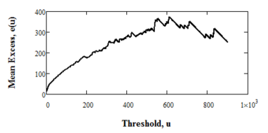
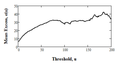
In Fig. 2 one can see plots of the mean excess function $\{(u,e(u)):X_{(1)}<u<X_{(n)}\}$, both for Enron and DBPL data sets. We may conclude that both data sets are heavy-tailed. Due to a linearity of the Enron-plot one may suggest that the Pareto model can be appropriate for the Enron email data. For DBPL data one cannot expect stationarity since the linear curve is changed by a nearly constant line. Hence, we may think that the distribution contains a mixture of an exponential and Pareto distributions. For large $u$ the plots look misleading due to rare observations exceeding such high thresholds.
The power law density may be determined by

$$f_{pl}(x)=(X_{(n-k)})^{\alpha}\alpha x^{-\alpha-1},$$ (12)

where $\int_{X_{(n-k)}}^{\infty}f_{pl}(x)dx=1$ holds.
The reciprocal of the tail index $\gamma=1/\alpha$ may be estimated by Hill’s estimator (Hill (1975))

$$\hat{\gamma}^{H}(n,k) = 1/k\sum_{i=1}^{k}\log X_{(n-i+1)}-\log X_{(n-k)}$$ (13)

and by the Ratio estimator. The latter is a generalization of the Hill’s one in a sense that instead of $X_{(n-k)}$ in (13) an arbitrary threshold $x_{n}>0$ is used, Markovich (2007). Both estimators may be applied to dependent data such as Markov chains, Novak (2002). Consistency of Hill’s estimator has been derived in Resnick and Starica (1998) for the $m$-dependent heavy-tailed stationary sequences. We apply also the Moment estimator which is a function of the Hill’s estimator

$$\hat{\gamma}^{M}_{n,k}=\hat{\gamma}^{H}(n,k)+1-0.5\left(1-(\hat{\gamma}^{H}(n,k))^{2}/S_{n,k})\right)^{-1},$$

where $S_{n,k}=(1/k)\sum_{i=1}^{k}\left(\log X_{(n-i+1)}-\log X_{(n-k)}\right)^{2}$. A survey of other estimators can be found in Markovich (2007) among others.
The number of the largest order statistics $k$ used in all estimators is estimated by a double bootstrap method, Danielsson et al. (2001). In Table 1 estimated values of the tail index for the Enron email and the DBLP data are shown. The number of bootstrap re-samples $B=500$ is used.

Table 1: Estimation of the tail index $\alpha$ by real data sets averaged over $500$ bootstrap re-samples.

Data	Sample	k	Hill	Ratio	Moment
	size
Enron	36692	1659	1.337	1.2182	1.023
DBPL	425957	2589	1.028	1.277	1.657

It is shown that all estimates of $\alpha$ are slightly larger than $1$ but smaller than $2$. This implies the infinite variance of the node degree distribution according to properties of regularly varying distributions (Breiman’s theorem), Embrechts et al. (1997), Markovich (2007). The fact that not all moments are finite confirms the heavy-tailed distributions of both underlying data sets. Since the tail index is larger for the Enron data, it follows from (8) that its distribution has lighter tail than the DBPL data.

Figure 3: The histogram and the power law density (12) for the Enron email data with tail index $\alpha=1.337$ (top) and for the DBPL data with $\alpha=1.277$ (bottom).

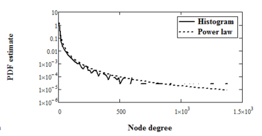
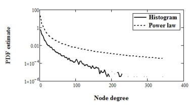
The comparison of the histogram and the power law density (12) for both data sets is shown in Fig. 3. One may conclude that the power law fits the Enron email data but not the DBPL data. This is in agreement with the mean excess function.
One cannot use the goodness-of-fit tests like Kolmogorov-Smirnov or von Mises-Smirnov tests to check the hypothesis regarding the power law. The reason is that the latter tests require samples of independent random variables. However, due to links between nodes, the node degrees are dependent.

3.2 Extremal index estimation

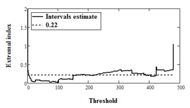
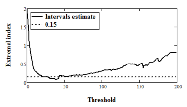
To estimate the extremal index $\theta$, we use the intervals estimator

$$\hat{\theta}_{n}(u) = \Big{\{}\begin{array}[]{ll}\min(1,\hat{\theta}_{n}^{1}(u)),\mbox{ if }\max\{T_{i}:1\leq i\leq N-1\}\leq 2,\\ \min(1,\hat{\theta}_{n}^{2}(u)),\mbox{ if }\max\{T_{i}:1\leq i\leq N-1\}>2,\end{array}$$

where

$$\hat{\theta}_{n}^{1}(u)=\frac{2(\sum_{i=1}^{N-1}T_{i})^{2}}{(N-1)\sum_{i=1}^{N-1}T_{i}^{2}},$$

and

$$\hat{\theta}_{n}^{2}(u)=\frac{2(\sum_{i=1}^{N-1}(T_{i}-1))^{2}}{(N-1)\sum_{i=1}^{N-1}(T_{i}-1)(T_{i}-2)},$$

proposed by Ferro and Segers (2003). Here,

$$N=\sum_{i=1}^{n}1(X_{i}>u)$$

is a number of exceedances of $u$ at time epochs $1\leq S_{1}<\ldots<S_{N}\leq n$ and the interexceedance times are given by $T_{i}=S_{i+1}-S_{i}$. The intervals estimator does not require the selection of any parameter apart of $u$ and demonstrates a good accuracy. In contrast, well-known nonparametric blocks and runs estimators require the size of blocks as an additional parameter to $u$, Beirlant et al. (2004).
In Fig. 4 the intervals estimates are shown for both data sets. The appropriate values of $\theta$ are selected corresponding to a stability interval of the curve $(u,\hat{\theta}_{n}(u))$. Since $1/\theta$ approximates the mean cluster size of exceedances of the thresholds, we may conclude that the Enron email data contains smaller clusters with $4-5$ nodes on average and the DBPL data $5-6$ nodes on average.

Figure 4: Intervals estimate of $\theta$ for the Enron email data (top) and the DBPL data (bottom): $\theta=0.22$ and $\theta=0.15$ are selected, respectively, as values corresponding to stability intervals of the curves.

3.3 First-hitting-time estimation

Using the obtained estimates $\theta\in\{0.22,0.15\}$, we evaluate the mean of the first hitting time and its distribution by means of (6) and (7), respectively.

Figure 5: The mean first hitting time of the Enron email and the DBPL data against the quantile level $1-\rho$: larger $1-\rho$ correspond to larger quantiles $x_{\rho}$ taken as thresholds and longer first hitting times.

Figure 6: The geometric model (15) of the normalized distribution $\theta^{2}P\{T^{*}(x_{\rho})=j\}$ of the first hitting time of the Enron email and the DBPL data corresponding to $95\%$ quantiles as thresholds.

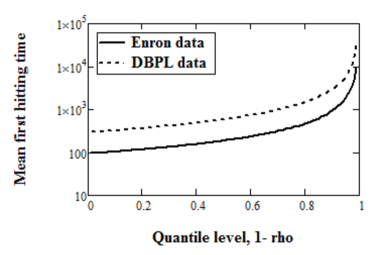
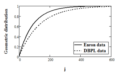
In Fig. 5 and 6 we use the following approximations

$$E\left(T^{*}(x_{\rho_{n}})\right)\approx 1/(\rho_{n}\theta^{3})$$

and

$$\theta^{2}P\{T^{*}(x_{\rho_{n}})=j\}\approx\rho_{n}\theta(1-\rho_{n}\theta)^{j-1},$$ (15)

respectively, that are valid for sufficiently large sample size $n$.
The $95\%$ quantiles $x_{\rho}$ ($\rho=0.05$) of the node degrees were used as thresholds.
Thus, we may conclude that for the DBPL data the mean time required to reach a node with degree larger than $u=x_{\rho}$ is longer than for the Enron email data. This reflects on the distributions, too. The distribution of the first hitting time of the DBPL data has heavier tail than the one of the Enron data.

3.4 Polynomial convergence rate of the Metropolis random walk

Using (10) and (11) as well as the tail index estimates, one can easily calculate the polynomial convergence rate of the Metropolis random walk. For example, for $\alpha=1.337$ w.r.t. the Enron data we get from (10) that $r=0.337$. To get the largest polynomial rate $v$ we select $\eta$ in (11) as small as possible within the interval $(0,2)$. For $\eta=0.01$ we get $v=33.7$. Similarly, for $\alpha=1.028$ w.r.t. the DBPL data we get $r=0.028$ and for the same $\eta$ we obtain $v=2.8$. This implies, that for the DBPL data whose tail distribution is heavier than the tail of the Enron, we get the slower polynomial convergence rate of the Metropolis random walk. Hence, the sampling by means of the Metropolis random walk could be more effective for the Enron email data rather than for the DBPL data.

4 Conclusions

We propose to evaluate the optimality of samplings in complex networks using new measures such as the extremal index, the distribution of the first hitting time and its mean. Considering real data of social networks we conclude that a heavier tail of the node degree distribution leads to (1) larger node clusters around the giant nodes, (2) slower convergence rate of the Metropolis random walk, and (3) a longer first hitting time to reach a large node.

References

- Andrieu et al. [2011] Andrieu, C., Jasra, A., Doucet, A., and Moral, P.D. (2011). On nonlinear markov chain monte carlo. Bernoulli, 17(3), 987–1014.
- Avrachenkov et al. [2010] Avrachenkov, K., Ribeiro, B., and Towsley, D. (2010). Improving random walk estimation accuracy with uniform restarts. In R. Kumar and D. Sivakumar (eds.), Algorithms and Models for the Web-Graph, volume 6516 of Lecture Notes in Computer Science, 98–109. Springer, Berlin Heidelberg.
- Beirlant et al. [2004] Beirlant, J., Goegebeur, Y., Teugels, J., and Segers, J. (2004). Statistics of Extremes: Theory and Applications. Wiley, Chichester, West Sussex.
- Clauset et al. [2009] Clauset, A., Shalizi, C.R., and Newman, M.E.J. (2009). Power-law distributions in empirical data. SIAM Rev., 51(4), 661 703.
- Danielsson et al. [2001] Danielsson, J., de Haan, L., Peng, L., and de Vries, C.G. (2001). Using a bootstrap method to choose the sample fraction in tail index estimation. Journal of Multivariate Analysis, 76(2), 226–248.
- Embrechts et al. [1997] Embrechts, P., Klüppelberg, C., and Mikosch, T. (1997). Modelling Extremal Events for Finance and Insurance. Springer, Berlin.
- Ferro and Segers [2003] Ferro, C. and Segers, J. (2003). Inference for clusters of extreme values. J. R. Statist. Soc. B., 65, 545–556.
- Hastings [1970] Hastings, W. (1970). Monte carlo sampling methods using markov chains and their applications. Biometrika, 57(1), 97–109.
- Hill [1975] Hill, B. (1975). A simple general approach to inference about the tail of a distribution. Annals of Statistics, 3, 1163–1174.
- Imbrenda et al. [September 24- 26, 2014] Imbrenda, C., Muscariello, L., and Rossi, D. (September 24- 26, 2014). Analyzing cacheable traffic in isp access networks for micro cdn applications via content-centric networking. 57–66.
- Jarner and Roberts [2007] Jarner, S. and Roberts, G.O. (2007). Convergence of heavy-tailed monte carlo markov chain algorithms. Scandinavian Journal of Statistics, 34(4), 781–815.
- Leadbetter [1983] Leadbetter, M.R. (1983). Probability theory and related fields. Zeitschrift f ur Wahrscheinlichkeitstheorie und Verwandte Gebiete, 65(2), 291–306.
- Leaflet [cited December 2014] Leaflet (cited December 2014). The one million tweet map. http://onemilliontweetmap.com/.
- Lee et al. [2012] Lee, C.H., Xu, X., and Eun, D.Y. (2012). Beyond random walk and metropolis-hastings samplers: Why you should not backtrack for unbiased graph sampling. CoRR.
- Leskovec and Krevl [2014] Leskovec, J. and Krevl, A. (2014). SNAP Datasets: Stanford large network dataset collection. http://snap.stanford.edu/data.
- Litvak et al. [2007] Litvak, N., Scheinhardt, W., and Volkovich, Y. (2007). In-degree and pagerank: Why do they follow similar power laws? Internet Mathematics, 4(2-3), 175–198.
- Markovich [2007] Markovich, N.M. (2007). Nonparametric Estimation of Univariate Heavy-Tailed Data. Wiley, Chichester.
- Markovich [2015] Markovich, N.M. (2015). Hitting times of threshold exceedances and their distributions. http://arxiv.org/abs/1501.01561, 1–6. Available at http://hal.inria.fr/hal-01054929.
- Mengersen and Tweedie [1996] Mengersen, K. and Tweedie, R. (1996). Rates of convergence of the hastings and metropolis algorithms. The Annals of Statistics, 24(1), 101–121.
- Metropolis et al. [1953] Metropolis, N., Rosenbluth, A., N.Rosenbluth, M., Teller, A.H., and Teller, E. (1953). Equation of state calculations by fast computing machines. The Journal of Chemical Physics, 21(6), 1087–1092.
- Newman [2006] Newman, M.E.J. (2006). Power laws, pareto distributions and zipf s law. arXiv:cond-mat/0412004v3 [cond-mat.stat-mech].
- Novak [2002] Novak, S.Y. (2002). Inference on heavy tails from dependent data. Siberian Adv. Math., 12(2), 73 96.
- Resnick and Starica [1998] Resnick, S.N. and Starica, J.S. (1998). Tail index estimation for dependent data. The Annals of Applied Probability, 8(4), 1156 1183.
- Roberts et al. [2006] Roberts, G.O., Rosenthal, J.S., Segers, J., and Sousa, B. (2006). Extremal indices, geometric ergodicity of markov chains, and mcmc. Scandinavian Journal of Statistics, 9, 213–229.
- Roberts and Smith [1994] Roberts, G.O. and Smith, A. (1994). Simple conditions for the convergence of the gibbs sampler and metropolis-hastings algorithms. Stochastic Processes and their Applications, 49, 207–216.
- Volkovich and Litvak [2010] Volkovich, Y. and Litvak, N. (2010). On the exceedance point process for a stationary sequence. Advances in Applied Probability, 42(2), 577–604.
- Volkovich et al. [2007] Volkovich, Y., Litvak, N., and Zwart, B. (2007). Measuring extremal dependencies in web graphs. Technical report, University of Twente.
- Volkovich et al. [2009] Volkovich, Y., Litvak, N., and Zwart, B. (2009). Extremal dependencies and rank correlations in power law networks. In J. Zhou (ed.), Complex 2009, volume Part II, LNICST 5, 1642 1653. Springer, Berlin Heidelberg NY.