Bayesian Estimation of Smooth Altimetric Parameters: Application to Conventional and Delay/Doppler Altimetry

Abstract

This paper proposes a new Bayesian strategy for the smooth estimation of altimetric parameters. The altimetric signal is assumed to be corrupted by a thermal and speckle noise distributed according to an independent and non identically Gaussian distribution. We introduce a prior enforcing a smooth temporal evolution of the altimetric parameters which improves their physical interpretation. The posterior distribution of the resulting model is optimized using a gradient descent algorithm which allows us to compute the maximum a posteriori estimator of the unknown model parameters. This algorithm presents a low computational cost which is suitable for real time applications. The proposed Bayesian strategy and the corresponding estimation algorithm are validated on both synthetic and real data associated with conventional and delay/Doppler altimetry. The analysis of real Jason-$2$ and Cryosat-$2$ waveforms shows an improvement in parameter estimation when compared to the state-of-the-art estimation algorithms.

I Introduction

A satellite altimeter is a nadir viewing radar that emits regular pulses and records the travel time, the magnitude and the shape of each return signal after reflection on the Earth’s surface. This reflected echo provides information about many parameters such as the range between the satellite and the observed scene (denoted by $\tau$), the significant wave height (denoted by SWH) and the wind speed (related to the echo’s amplitude $P_{u}$). However, altimetric waveforms are corrupted by speckle noise that reduces the quality of the retrieved geophysical parameters. Therefore, many recent studies and missions have been focusing on improving the quality of these estimated parameters by reducing the noise effect. We distinguish between two approaches that have been focusing on improving the altimetric technology or improving the processing of the available data. The first approach is based on reducing the measurement noise of conventional altimeters (such as Topex and Poseidon-3) by increasing the number of observations (looks). This can be achieved by keeping the same conventional technology and improving the altimeter characteristics (as for AltiKa [1, 2, 3]), or by using a new delay/Doppler processing [4] that results in a different echo’s shape [5, 6, 7]. The second approach processes the available data by using improved models for the altimetric echoes [8, 9, 10, 11] or improved estimation algorithms [12, 13, 14].

Following this second approach, the goal of this paper is to elaborate a new Bayesian model and its estimation algorithm accounting for the smooth evolution of altimetric signals. Usual methods for parameter estimation are based on maximum-likelihood [15] or weighted [12, 16] and unweighted least squares (LS) approaches [9, 6, 7]. Most existing algorithms consider altimetric echoes independently and estimate one set of parameters per echo. However, it is well known that adjacent echoes share similar characteristics because of their physical nature. This correlation has been considered in [12] which processed a set of echoes by imposing a spline evolution for the epoch parameter $\tau$. However, this method was developed by fixing the significant wave height for the whole set of echoes. In [13], the authors proposed a three-step algorithm that reduces the range noise by first estimating three altimetric parameters (SWH, $\tau$ and $P_{u}$), then filtering the estimated SWH using a Gaussian filter and finally re-estimating the epoch $\tau$ while fixing SWH. This last algorithm is flexible since it does not enforce the parameter SWH to be constant. However, it requires to use a sequential estimator whose computational cost can be prohibitive. Moreover, the algorithm of [13] requires the characterization of a Gaussian filter for SWH which has been chosen empirically. Also, it is interesting to note that the algorithms developed in [12, 13] have shown interesting properties especially in reducing the variance of the estimated altimetric parameters which encourages the consideration of the echo’s correlation to improve parameter estimation.

The first contribution of this paper is the elaboration of a hierarchical Bayesian model that allows smooth estimation of altimetric parameters by considering the correlation between successive altimetric echoes. Each altimetric echo is assumed to be corrupted by an additive, independent and non identically Gaussian noise [17] whose mean is the thermal noise. This noise model generalizes the independent and identically distributed (i.i.d.) Gaussian noise that is generally assumed when considering an un-weighted LS approach [9, 6]. The proposed approach allows the estimation of the noise parameters from the data which brings additional robustness compared to existing algorithms and allows the processing of different kinds of data. The parameters of interest of the proposed model (i.e., SWH, $\tau$, $P_{u}$) are assigned priors enforcing a smooth evolution between consecutive signals which improves their estimation. This prior is defined from the discrete Laplacian of the different parameters. It has shown increasing interest for many problems such as image deconvolution [18, 19], hyperspectral unmixing [20] and medical imaging [21]. Note that the proposed Bayesian hierarchy is generic in the sense that it can be applied to both conventional altimetry (CA) and delay/Doppler altimetry (DDA).

The second contribution of this paper is the derivation of an estimation algorithm for the altimetric and noise parameters associated with the proposed hierarchical Bayesian model. The minimum mean square error (MMSE) and maximum a posteriori (MAP) estimators of these parameters cannot be easily computed from the obtained joint posterior. This problem has been solved in [22] by drawing samples distributed according to this posterior using Markov chain Monte Carlo (MCMC) methods. More precisely, an Hamiltonian Monte Carlo (HMC) algorithm was used for its good mixing properties for high-dimensional vectors [23]. The HMC algorithm provided good estimation results and will be briefly recalled in this paper. However, the resulting HMC-based estimators have a high computational complexity which can be penalizing for real time applications. In this paper, we propose an algorithm that significantly reduces this computational cost by using a gradient descent approach. More precisely, a coordinate descent algorithm [24, 20] is used to sequentially update the noise and altimetric parameters. This algorithm uses a natural gradient approach [25], weighting the gradient direction by the Fisher information matrix and leading to a fast convergence. The proposed Bayesian model and estimation algorithm are validated using synthetic and real echoes acquired during the Jason-$2$ and Cryosat-$2$ missions. The obtained results are very promising and confirm the accuracy of the proposed Bayesian model and its associated algorithm.

The paper is organized as follows. Section II presents the different models used for CA and DDA. The proposed hierarchical Bayesian model and its estimation algorithm are introduced in Sections III and IV. Section V is devoted to testing and validating the proposed technique using synthetic data with controlled ground truth. Section VI shows results obtained using real data resulting from Jason-2 and Cryosat-2 missions. Conclusions and future work are finally reported in Section VII.

II Altimetric models

This section introduces the altimetric models used for CA and DDA that are characterized by three altimetric parameters: the significant wave height SWH, the epoch $\tau$ and the amplitude $P_{u}$.

II-A Conventional and Brown models

In CA, the mean power of the altimetric echo $s(t)$ is expressed by a convolution of three terms that are the probability density function (PDF) of the heights of the specular scatterers, the point target response (PTR) of the radar and the flat surface impulse response (FSIR) as follows [8, 31, 9]

$$s(t)=\textrm{FSIR}(t)*\textrm{PDF}(t)*\textrm{PTR}_{T}(t)$$ (1)

with

$$\textrm{FSIR}(t)=P_{u}\exp{\left[-\frac{4c}{\gamma h}\left(t-\tau_{s}\right)\right]}U\left(t-\tau_{s}\right)$$ (2)

$$\textrm{PDF}(t)=\frac{1}{\sqrt{2\pi}\sigma_{s}}\exp{\left(-\frac{t^{2}}{2\sigma_{s}^{2}}\right)}$$ (3)

$$\textrm{PTR}_{T}(t)={\left|\frac{\sin{\left(\pi\frac{t}{T}\right)}}{\pi\frac{t}{T}}\right|}^{2}$$ (4)

where $\sigma_{s}=\frac{\textrm{SWH}}{2c}$, $t$ is the time, $\tau_{s}$ is the epoch expressed in seconds, $c$ is the speed of light, $T$ is the time resolution, $\gamma$ is an antenna beamwidth parameter, $h$ is the minimum satellite-surface distance and $U(.)$ denotes the Heaviside function. This model has been considered for parameter estimation in many studies such as [6, 16]. However, the numerical computation of the double convolution (1) leads to a high computational cost when processing a large amount of altimetric data. Therefore, a simplified analytical model known as the Brown model (BM) is often considered. The BM is obtained by assuming a centered Gaussian approximation (with a standard-deviation equals to $\sigma_{p}$) for the squared cardinal sine $\textrm{PTR}_{T}$, leading to [8, 9]

$$s(t)=\frac{P_{u}}{2}\left[1+\textrm{erf}\left(\frac{t-\tau_{s}-\alpha\sigma_{c}^{2}}{\sqrt{2}\sigma_{c}}\right)\right]\exp\left[-\alpha\left(t-\tau_{s}-\frac{\alpha\sigma_{c}^{2}}{2}\right)\right]$$ (5)

where

$$\qquad\sigma_{c}^{2}=\left(\frac{\textrm{SWH}}{2c}\right)^{2}+\sigma_{p}^{2}$$ (6)

and where $\textrm{erf}\left(t\right)=\frac{2}{\sqrt{\pi}}\int_{0}^{t}e^{-z^{2}}\,dz$ stands for the Gaussian error function, $\alpha$ and $\sigma_{p}^{2}$ being two known parameters (depending on the satellite and on the Gaussian approximation of the PTR). The model (5) is clearly more attractive than (1) for designing simple estimation algorithms.

II-B Delay/Doppler altimetry

DDA aims at reducing the measurement noise and increasing the along-track resolution in comparison with CA. The mean power of a delay/Doppler echo can be expressed as the convolution of three terms: the time/frequency FSIR, the PDF of the heights of the specular scatterers and the time/frequency PTR as follows [17, 32, 6, 7]

$$P(t,f)=\textrm{FSIR}(t,f)*\textrm{PDF}(t)*\textrm{PTR}(t,f)$$ (7)

with

$$\textrm{PTR}(t,f)=\textrm{PTR}_{T}(t)\textrm{PTR}_{F}(f),\;\;\textrm{PTR}_{F}(f)={\left|\frac{\sin{\left(\pi\frac{f}{F}\right)}}{\pi\frac{f}{F}}\right|}^{2}$$ (8)

where $F$ is the frequency resolution. The FSIR is given by [6]

$$\textrm{FSIR}(t,q)=\frac{P_{u}}{\pi}\exp{\left[-\frac{4c}{\gamma h}\left(t-\tau_{s}\right)\right]}\,U\left(t-\tau_{s}\right)$$

$$\times\left[\phi_{t,q+1}(\tau_{s})-\phi_{t,q}(\tau_{s})\right]$$ (9)

with

$$\phi_{t,q}(\tau_{s})=\operatorname{Re}\left[\textrm{arctan}\left(\frac{y_{q}}{\sqrt{\rho^{2}(t-\tau_{s})-y_{q}^{2}}}\right)\right]$$ (10)

where $q=1,\cdots,Q$, $Q$ being the number of Doppler beams ($Q=64$ for Cryosat-$2$), $\rho(t)=\sqrt{hct}$ is the radius of the propagation circles (iso-range circles), $y_{q}=\frac{h\lambda}{2v_{s}}f_{q}$ is the ordinate of the $q^{\textrm{th}}$ Doppler beam, $f_{q}=\left(q-32.5\right)F$ is the $q^{\textrm{th}}$ Doppler frequency ($32.5$ is introduced to obtain a central beam in the case where $Q=64$), $v_{s}$ is the satellite velocity, $\lambda$ is the wavelength and $\operatorname{Re}(x)$ denotes the real part of the complex number $x$ (the interested reader is invited to consult [6] for more details about this formula). The double convolution (7) leads to a 2-D delay/Doppler map (DDM). The analysis of the DDA waveform is based on a multi-look echo obtained by applying Doppler processing (slant range correction and multi-looking) to the DDM (see [4, 5]). The resulting multi-look delay/Doppler signal can be written

$$s(t)=\sum_{q=1}^{Q}P\left(t-\delta t_{q},f_{q}\right)$$ (11)

where $\delta t_{q}$ is the delay compensation expressed in seconds. Note finally that the discrete altimetric echo (for CA, BM, and DDA) is gathered in the vector ${\boldsymbol{s}}=\left(s_{1},\cdots,s_{K}\right)^{T}$, where $K=128$ gates and $s_{k}=s\left(kT\right)$.

II-C Noise model

The altimetric echoes are corrupted by a speckle noise whose influence is reduced by averaging, on-board the satellite, a sequence of $L$ consecutive echoes. This operation reduces the noise variance by $\sqrt{L}$ when assuming pulse-to-pulse statistical independence between the averaged echoes. Considering the central limit theorem and using the fact that the averaging is conducted on a large number of echoes, the resulting noise sequence can be approximated by a Gaussian distribution. This approximation has been successfully adopted in the altimetric community [17, 33, 16] and is implicitly used in the well known least squares estimation algorithms [34, 6, 12, 13]. Therefore, this paper considers that the altimetric waveform is corrupted by an additive Gaussian noise as follows

$${\boldsymbol{y}}_{m}={\boldsymbol{s}}_{m}\left(\boldsymbol{\Theta}_{m}\right)+{\boldsymbol{e}}_{m},\textrm{ with }{\boldsymbol{e}}_{m}\sim{\mathcal{N}}\left(\mu_{m}\boldsymbol{1}_{K},\boldsymbol{\Sigma}_{m}\right)$$ (12)

where ${\boldsymbol{y}}_{m}$ (resp. ${\boldsymbol{s}}_{m}$) is a ($K\times 1$) vector representing the $m$th observed echo (resp. altimetric model), $\boldsymbol{\Theta}_{m}=\left[\theta_{1}(m),\theta_{2}(m),\theta_{3}(m)\right]=\left[\textrm{SWH}(m),\tau(m),P_{u}(m)\right]$ is a ($1\times 3$) vector containing the $3$ altimetric parameters $\textrm{SWH},\tau,P_{u}$ for the $m$th echo, ${\boldsymbol{e}}_{m}$ is an independent and non identically Gaussian noise with mean vector $\mu_{m}\boldsymbol{1}_{K}$ representing the thermal noise (where $\boldsymbol{1}_{K}$ is a $K\times 1$ vector of $1$), and diagonal covariance matrix $\boldsymbol{\Sigma}_{m}=\textrm{diag}\left(\boldsymbol{\sigma}^{2}_{m}\right)$ with $\boldsymbol{\sigma}^{2}_{m}=\left(\sigma^{2}_{m1},\cdots,\sigma^{2}_{mK}\right)^{T}$ a ($K\times 1$) vector containing the noise variances of the $m$th echo. Note that the thermal noise parameter is sometimes represented by an additive constant that is added to the altimetric model ${\boldsymbol{s}}_{m}\left(\boldsymbol{\Theta}_{m}\right)$. In the proposed model, this parameter has been included in the noise sequence ${\boldsymbol{e}}_{m}$ of (12) where it represents the noise mean $\mu_{m}$. The next section introduces the Bayesian model associated with a set of $M$ successive echoes considered in this paper.

III Hierarchical Bayesian model

This section introduces a hierarchical Bayesian model for estimating the parameters of $M$ successive altimetric echoes. The Bayesian approach assigns prior distributions to the unknown parameters summarizing the prior knowledge about these parameters. More precisely, if $f\left({\boldsymbol{x}}\right)$ denotes the prior distribution assigned to the parameter ${\boldsymbol{x}}$, the Bayesian approach computes the posterior distribution of ${\boldsymbol{x}}$ using Bayes rule

$$f({\boldsymbol{x}}|{\boldsymbol{Y}})=\frac{f({\boldsymbol{Y}}|{\boldsymbol{x}})f({\boldsymbol{x}})}{f({\boldsymbol{Y}})}\propto f({\boldsymbol{Y}}|{\boldsymbol{x}})f({\boldsymbol{x}})$$ (13)

where $\propto$ means “proportional to” and $f({\boldsymbol{Y}}|{\boldsymbol{x}})$ is the likelihood of the observation vector ${\boldsymbol{Y}}$. The vector ${\boldsymbol{x}}$ is then estimated from this distribution by computing its mean (MMSE estimator) or its maximum (MAP estimator). The following sections introduce the likelihood and the prior distributions considered in this paper. The unknown parameters of the proposed model include the thermal noise represented by an ($M\times 1$) vector $\boldsymbol{\mu}$, the ($K\times M$) matrix $\boldsymbol{\Lambda}=\left[\boldsymbol{\sigma}^{2}_{1},\cdots,\boldsymbol{\sigma}^{2}_{M}\right]$ containing the noise variances associated with the considered $M$ echoes, and the ($M\times 3$) matrix gathering the $3$ altimetric parameters (SWH, $\tau$ and $P_{u}$) of the $M$ echoes.

III-A Likelihood

The observation model defined in (12) and the Gaussian properties of the noise sequence ${\boldsymbol{e}}_{m}$ yield

$$f({\boldsymbol{y}}_{m}|\boldsymbol{\Theta}_{m},\mu_{m},\boldsymbol{\Sigma}_{m})\propto{\left(\frac{1}{\prod_{k=1}^{K}\sigma^{2}_{mk}}\right)}^{\frac{1}{2}}\exp\left\{-\frac{1}{2}{\boldsymbol{x}}_{m}^{T}\boldsymbol{\Sigma}_{m}^{-1}{\boldsymbol{x}}_{m}\right\}$$ (14)

where ${\boldsymbol{x}}_{m}={\boldsymbol{y}}_{m}-{\boldsymbol{s}}_{m}-\mu_{m}\boldsymbol{1}_{K}$, and ${\boldsymbol{x}}_{m}\left(\boldsymbol{\Theta}_{m}\right)$ (resp. ${\boldsymbol{s}}_{m}\left(\boldsymbol{\Theta}_{m}\right)$) has been denoted by ${\boldsymbol{x}}_{m}$ (resp. ${\boldsymbol{s}}_{m}$) for brevity. Assuming independence between the observations leads to

$$f({\boldsymbol{Y}}|\boldsymbol{\Theta},\boldsymbol{\mu},\boldsymbol{\Lambda})\propto\prod_{m=1}^{M}{f({\boldsymbol{y}}_{m}|\boldsymbol{\Theta}_{m},\mu_{m},\boldsymbol{\Sigma}_{m})}$$ (15)

where $\boldsymbol{\Theta}=\left[\boldsymbol{\theta}_{1},\boldsymbol{\theta}_{2},\boldsymbol{\theta}_{3}\right]$ is an ($M\times 3$) matrix containing the altimetric parameters of $M$ echoes, $\boldsymbol{\mu}=\left(\mu_{1},\cdots,\mu_{M}\right)^{T}$ is an ($M\times 1$) vector containing the noise means and $\boldsymbol{\Lambda}=\left[\boldsymbol{\sigma}^{2}_{1},\cdots,\boldsymbol{\sigma}^{2}_{M}\right]$ is a ($K\times M$) matrix containing the noise variances.

III-B Priors for the altimetric parameters

The altimetric parameters are assigned priors enforcing a smooth evolution for successive waveforms. The considered priors constrain the derivatives of the altimetric parameters to have small values. This can be done by assigning a Gaussian distribution to the second derivative of the altimetric parameter $\boldsymbol{\theta}_{i}$ as follows

$$f(\boldsymbol{\theta}_{i}|\epsilon^{2}_{i})\propto\left(\frac{1}{\epsilon_{i}^{2}}\right)^{M/2}\exp{\left(-\frac{1}{2\epsilon_{i}^{2}}\left\|{\boldsymbol{D}}\boldsymbol{\theta}_{i}\right\|^{2}\right)}$$ (16)

for $i\in\left\{1,\cdots,3\right\}$, where $\epsilon^{2}_{i}$ is an hyperparameter, $||\cdot||$ denotes the standard $l_{2}$ norm such that $||{\boldsymbol{x}}||^{2}={\boldsymbol{x}}^{T}{\boldsymbol{x}}$, and ${\boldsymbol{D}}$ is the discrete Laplacian operator. This prior has been referred to as simultaneous autoregression (SAR) or conditional autoregression (CAR) in the image deconvolution context [18, 19]. It has also been used for different problems such as spectral unmixing of hyperspectral images [20], medical imaging applications [21] or spectroscopy applications [35]. The main originality of this work is to consider this prior for the parameters of altimetric waveforms.

III-C Prior for the noise parameters

The noise parameters introduced in (12) are also estimated by the proposed estimation algorithm. The absence of knowledge about the noise means (which represent the thermal noise) and covariances can be issued by choosing a non informative priors for these parameters. More precisely, we consider the following conjugate Gaussian prior with a large variance for the noise mean

$$f(\boldsymbol{\mu}|\psi^{2})\sim{\mathcal{N}}\left(\boldsymbol{0}_{M},\psi^{2}\mathbf{I}_{M}\right)$$ (17)

where $\mathbf{I}_{M}$ is the ($M\times M$) identity matrix, $\boldsymbol{0}_{M}$ is an ($M\times 1$) vector of $0$ and $\psi^{2}$ is a fixed large variance ($\psi^{2}=10^{2}$ in our simulations). Considering the noise covariance matrix, we have first to note that in the case of speckle noise, these variances depend on the echo’s shape at each instant, i.e., the variances change from one echo to the other. However, we are generally interested in parameters estimated with a frequency of $1$ Hz, i.e., we consider that the physical parameters do not change significantly in $1$ second. This assumption means that the shapes of successive echoes acquired within a time interval of $1$ s do not change significantly and thus that the noise variances are almost the same for these echoes. Therefore, we consider that the noise variance is constant for each $r=20$ successive echoes. This means that $\sigma^{2}_{(n-1)r+1,k}=\cdots=\sigma^{2}_{nr,k}$ for $n\in\left\{1,\cdots,N\right\}$, with $N=\frac{M}{r}$ (note that the general case is obtained by considering $r=1$). After assuming prior independence between the noise variances $\sigma^{2}_{nr,k}$, the non informative scale prior of $\boldsymbol{\Lambda}$ is defined as

$$f\left(\boldsymbol{\Lambda}\right)=\prod_{n=1}^{N}{\prod_{k=1}^{K}{\frac{1}{\sigma^{2}_{nr,k}}\mathbb{I}_{\mathbb{R}^{+}}\left(\sigma^{2}_{nr,k}\right)}}$$ (18)

where $\mathbb{I}_{\mathbb{R}^{+}}(.)$ is the indicator of the set $\mathbb{R}^{+}$.

III-D Hyperparameter priors

The hyperparameters $\epsilon_{i}^{2},i\in\left\{1,\cdots,3\right\}$ are assigned independent inverse gamma distributions as follows

$$\epsilon_{i}^{2}\ \sim{\mathcal{I}}{\mathcal{G}}\left(a_{i},b_{i}\right)$$ (19)

where $\sim$ means “is distributed according to” and $a_{i}$, $b_{i}$ are fixed hyperparameters that depend on the dynamic magnitude of the $i$th altimetric parameter [35].

III-E Marginalized posterior distribution

The proposed Bayesian model includes the parameters $\boldsymbol{\Theta},\boldsymbol{\mu},\boldsymbol{\Lambda}$ and the hyperparameters $\epsilon_{i}^{2},i\in\left\{1,\cdots,3\right\}$ which is summarized in the directed acyclic graph (DAG) displayed in Fig. 1. The joint posterior distribution of this Bayesian model can be computed from the following hierarchical structure

$$f\left(\boldsymbol{\Theta},\boldsymbol{\mu},\boldsymbol{\Lambda},\boldsymbol{\epsilon}|{\boldsymbol{Y}}\right)\propto f({\boldsymbol{Y}}|\boldsymbol{\Theta},\boldsymbol{\mu},\boldsymbol{\Lambda})f\left(\boldsymbol{\Theta},\boldsymbol{\mu},\boldsymbol{\Lambda},\boldsymbol{\epsilon}\right)$$ (20)

with

$$f\left(\boldsymbol{\Theta},\boldsymbol{\mu},\boldsymbol{\Lambda},\boldsymbol{\epsilon}\right) = f\left(\boldsymbol{\mu}|\psi^{2}\right)f\left(\boldsymbol{\Lambda}\right)\prod_{i=1}^{3}{f(\boldsymbol{\theta}_{i}|\epsilon^{2}_{i})f(\epsilon^{2}_{i}|a_{i},b_{i})}$$ (21)

where we have assumed a priori independence between the altimetric parameters and hyperparameters. This distribution can be marginalized with respect to (w.r.t.) $\boldsymbol{\epsilon}$ as follows

$$f\left(\boldsymbol{\Theta},\boldsymbol{\mu},\boldsymbol{\Lambda}|{\boldsymbol{Y}}\right) \propto f({\boldsymbol{Y}}|\boldsymbol{\Theta},\boldsymbol{\mu},\boldsymbol{\Lambda})f\left(\boldsymbol{\mu}|\psi^{2}\right)f\left(\boldsymbol{\Lambda}\right)\prod_{i=1}^{3}{\left[\int{f(\boldsymbol{\theta}_{i}|\epsilon^{2}_{i})f(\epsilon^{2}_{i}|a_{i},b_{i})}d\epsilon^{2}_{i}\right]}$$ (22)

$$\propto f({\boldsymbol{Y}}|\boldsymbol{\Theta},\boldsymbol{\mu},\boldsymbol{\Lambda})f\left(\boldsymbol{\mu}|\psi^{2}\right)f\left(\boldsymbol{\Lambda}\right)\prod_{i=1}^{3}{f\left(\boldsymbol{\theta}_{i}|a_{i},b_{i}\right)}$$

where

$$f\left(\boldsymbol{\theta}_{i}|a_{i},b_{i}\right)\propto\left(\frac{\left\|{\boldsymbol{D}}\boldsymbol{\theta}_{i}\right\|^{2}}{2}+b_{i}\right)^{-a_{i}-M/2}.$$ (23)

The advantage of this marginalization is to get rid of the hyperparameter vector $\boldsymbol{\epsilon}$ and thus to make the estimation procedure more robust. However, even with this simplification, the MMSE and MAP estimators associated with the marginalized posterior (22) are not easy to determine mainly because of the nonlinearities relating the noiseless altimetric waveform ${\boldsymbol{s}}_{m}$ and the parameters of interest ($\tau$ and SWH). In [22], an MCMC algorithm was proposed to sample the joint posterior distribution of a similar Bayesian model. The generated samples were then used to compute the MMSE parameter estimators (see Appendix -A for more details about this algorithm). However, this MCMC algorithm has a high computational complexity which can be penalizing for real time applications. In this paper, we propose an alternative based on an optimization technique maximizing the marginalized posterior (22) w.r.t. the parameters of interest (or equivalently, minimizing the negative log-posterior $-\textrm{log}[p(\boldsymbol{\Theta},\boldsymbol{\mu},\boldsymbol{\Lambda}|{\boldsymbol{Y}})]$ defined in (22)). The mode of the posterior distribution (22) is classically referred to as marginalized MAP estimator of ($\boldsymbol{\Theta},\boldsymbol{\mu},\boldsymbol{\Lambda}$).

Figure 1: DAG for the parameter and hyperparameter priors (the fixed parameters appear in boxes).

IV Coordinate descent algorithm

This section describes a gradient descent algorithm maximizing the marginalized posterior (22) w.r.t. the noise and altimetric parameters, i.e., determining the marginal MAP estimator of ($\boldsymbol{\Theta},\boldsymbol{\mu},\boldsymbol{\Lambda}$). As explained before, maximizing (22) w.r.t. ($\boldsymbol{\Theta},\boldsymbol{\mu},\boldsymbol{\Lambda}$) reduces to minimizing the negative log-posterior defined as (after removing unnecessary constants)

$$\mathcal{C}\left(\boldsymbol{\Theta},\boldsymbol{\mu},\boldsymbol{\Lambda}\right) = \left(\frac{r}{2}+1\right)\sum_{k=1}^{K}{\sum_{n=1}^{N}{\log\sigma_{nr,k}^{2}}}+\sum_{m=1}^{M}{\frac{{\boldsymbol{x}}_{m}^{T}\boldsymbol{\Sigma}_{m}^{-1}{\boldsymbol{x}}_{m}}{2}}$$ (24)

$$+ \sum_{i=1}^{3}{\left(a_{i}+\frac{M}{2}\right)\log\left(\frac{\left\|{\boldsymbol{D}}\boldsymbol{\theta}_{i}\right\|^{2}}{2}+b_{i}\right)}+\sum_{m=1}^{M}{\frac{\mu_{m}^{2}}{2\psi^{2}}}.$$

Because of the large number of parameters in ($\boldsymbol{\Theta},\boldsymbol{\mu},\boldsymbol{\Lambda}$), we propose a coordinate descent algorithm [24, 20] that sequentially updates the different parameters. More precisely, the algorithm estimates the altimetric and noise parameters iteratively. In each step, the parameters of interest are estimated while holding the other parameters fixed. This process is repeated until the algorithm has converged to a local minimum of the cost function $\mathcal{C}(\boldsymbol{\Theta},\boldsymbol{\mu},\boldsymbol{\Lambda})$. The main steps of the resulting algorithm are described in Algo. 1. The next sections describe the sub-optimization procedures maximizing the cost function $\mathcal{C}(\boldsymbol{\Theta},\boldsymbol{\mu},\boldsymbol{\Lambda})$ w.r.t. the altimetric and noise parameters. A convergence diagnosis is also provided to study the convergence of the proposed approach.

Algorithm 1 Gradient descent algorithm

1:  Initialization

2:  Initialize parameters $\boldsymbol{\theta}_{i}^{(0)},$ for $i\in\left\{1,\cdots,3\right\}$, $\boldsymbol{\mu}^{(0)}$, $\boldsymbol{\Lambda}^{(0)}$ and $t=1$

3:  conv$=0$,

4:  Parameter update

5:  while conv$=0$ do

6:     Update $\boldsymbol{\theta}_{i}^{(t)},$ for $i\in\left\{1,\cdots,3\right\}$ according to (25)

7:     Update $\boldsymbol{\mu}^{(t)}$ according to (31)

8:     Update $\boldsymbol{\Lambda}^{(t)}$ according to (34)

9:     Set conv$=1$ if the convergence criteria are satisfied

10:     t = t + 1

11:  end while

IV-1 Natural gradient for altimetric parameters

In order to ensure a fast estimation of the altimetric parameters, we propose to use the natural gradient algorithm to minimize $\mathcal{C}$ w.r.t. $\boldsymbol{\Theta}$ [25]. This gradient algorithm is also known as Fisher scoring approach since it weights the gradient direction by the Fisher information matrix of the parameters [26, 10]. The resulting descent algorithm updates the parameters in a Riemannian space resulting in a fast convergence to a local minimum of the objective function [27, 28]. Denote as $\boldsymbol{\gamma}=\left(\boldsymbol{\theta}_{1}^{T},\boldsymbol{\theta}_{2}^{T},\boldsymbol{\theta}_{3}^{T}\right)^{T}$ the ($3M\times 1$) vector gathering the altimetric parameters. The proposed algorithm updates this vector as follows

$$\boldsymbol{\gamma}^{(t+1)}=\boldsymbol{\gamma}^{(t)}-{\boldsymbol{F}}^{-1}\left(\boldsymbol{\gamma}^{(t)}\right)\nabla\mathcal{C}\left(\boldsymbol{\gamma}^{(t)}\right)$$ (25)

where $\nabla\mathcal{C}\left(\boldsymbol{\gamma}^{(t)}\right)$ denotes the gradient of the cost function $\mathcal{C}$ given by

$$\nabla\mathcal{C}=\frac{\partial\mathcal{C}}{\partial\boldsymbol{\gamma}}=\left[\left(\frac{\partial\mathcal{C}}{\partial\boldsymbol{\theta}_{1}}\right)^{T},\left(\frac{\partial\mathcal{C}}{\partial\boldsymbol{\theta}_{2}}\right)^{T},\left(\frac{\partial\mathcal{C}}{\partial\boldsymbol{\theta}_{3}}\right)^{T}\right]^{T}$$ (26)

with

$$\frac{\partial\mathcal{C}}{\partial\boldsymbol{\theta}_{i}}=-\left(\frac{\partial{\boldsymbol{s}}_{1}^{T}}{\partial\theta_{1i}}\boldsymbol{\Sigma}_{1}^{-1}{\boldsymbol{x}}_{1},\cdots,\frac{\partial{\boldsymbol{s}}_{M}^{T}}{\partial\theta_{Mi}}\boldsymbol{\Sigma}_{M}^{-1}{\boldsymbol{x}}_{M}\right)^{T}+\left(a_{i}+\frac{M}{2}\right)\left(\frac{{\boldsymbol{D}}^{T}{\boldsymbol{D}}\boldsymbol{\theta}_{i}}{\frac{\left\|{\boldsymbol{D}}\boldsymbol{\theta}_{i}\right\|^{2}}{2}+b_{i}}\right).$$ (27)

The Fisher information matrix ${\boldsymbol{F}}\left(\boldsymbol{\gamma}^{(t)}\right)$ can be decomposed as the following block matrix

$${\boldsymbol{F}}=\left[\begin{array}[]{ccc}{\boldsymbol{F}}_{1}&{\boldsymbol{F}}_{12}&{\boldsymbol{F}}_{13}\\ {\boldsymbol{F}}_{12}&{\boldsymbol{F}}_{2}&{\boldsymbol{F}}_{23}\\ {\boldsymbol{F}}_{13}&{\boldsymbol{F}}_{23}&{\boldsymbol{F}}_{3}\end{array}\right]$$ (28)

with

$${\boldsymbol{F}}_{ij} = \textrm{diag}\left(\frac{\partial{\boldsymbol{s}}_{1}^{T}}{\partial\theta_{1i}}\boldsymbol{\Sigma}_{1}^{-1}\frac{\partial{\boldsymbol{s}}_{1}}{\partial\theta_{1j}},\cdots,\frac{\partial{\boldsymbol{s}}_{M}^{T}}{\partial\theta_{Mi}}\boldsymbol{\Sigma}_{M}^{-1}\frac{\partial{\boldsymbol{s}}_{M}}{\partial\theta_{Mj}}\right)$$

$${\boldsymbol{F}}_{i} = {\boldsymbol{F}}_{ii}+\left(a_{i}+\frac{M}{2}\right)\left[\frac{\left(\frac{\left\|{\boldsymbol{D}}\boldsymbol{\theta}_{i}\right\|^{2}}{2}+b_{i}\right){\boldsymbol{D}}^{T}{\boldsymbol{D}}-\left({\boldsymbol{D}}^{T}{\boldsymbol{D}}\boldsymbol{\theta}_{i}\right)\left({\boldsymbol{D}}^{T}{\boldsymbol{D}}\boldsymbol{\theta}_{i}\right)^{T}}{\left(\frac{\left\|{\boldsymbol{D}}\boldsymbol{\theta}_{i}\right\|^{2}}{2}+b_{i}\right)^{2}}\right].$$ (29)

Note that the derivatives required to compute the elements of ${\boldsymbol{F}}$ are the same as those required to compute $\nabla\mathcal{C}$. Therefore, the only additional computation w.r.t. a steepest descent approach is the matrix inversion in (25). Note also that this matrix inversion is faster than a new evaluation of the altimetric model necessary for a new update of $\boldsymbol{\gamma}$ in a steepest descent algorithm. Therefore, it is better to add this inversion and reduce the number of iterations, instead of using a simple steepest descent approach that usually requires a lot of iterations to converge resulting in a high computational cost.

IV-2 Updating the noise parameters

Maximizing the marginalized posterior distribution (22) w.r.t. the noise parameters (means and variances) can be achieved by considering a coordinate descent algorithm. This approach reduces to maximizing the conditional distributions associated with each noise parameter. Using (15) and (17), it can be easily shown that the conditional distribution of the noise mean is the following Gaussian distribution

$$\mu_{m}|{\boldsymbol{y}}_{m},\boldsymbol{\Theta}_{m},\boldsymbol{\Sigma}_{m},\psi^{2}\sim{\mathcal{N}}\left(\overline{\mu_{m}},\frac{1}{\psi^{-2}+\sum_{k=1}^{K}\sigma_{mk}^{-2}}\right)$$ (30)

with

$$\overline{\mu_{m}}=\frac{\sum_{k=1}^{K}\frac{y_{mk}-s_{mk}}{\sigma_{mk}^{2}}}{\psi^{-2}+\sum_{k=1}^{K}\sigma_{mk}^{-2}}.$$ (31)

Therefore, the parameter vector $\boldsymbol{\mu}$ can be updated using (31) which is the maximum of the Gaussian distribution (30). Similarly, it can be shown using (15) and (18) that

$$f\left(\boldsymbol{\Lambda}|{\boldsymbol{Y}},\boldsymbol{\Theta},\boldsymbol{\mu}\right)=\prod_{n=1}^{N}{\prod_{k=1}^{K}{f\left(\sigma_{nr,k}^{2}|{\boldsymbol{Y}}_{:k},\boldsymbol{\Theta}_{k:},\boldsymbol{\mu}\right)}}$$ (32)

and that $\sigma_{nr,k}^{2}|{\boldsymbol{Y}}_{:k},\boldsymbol{\Theta}_{k:},\boldsymbol{\mu}$ is distributed according to the following inverse-gamma distribution

$$\sigma_{nr,k}^{2}|{\boldsymbol{Y}}_{:k},\boldsymbol{\Theta}_{k:},\boldsymbol{\mu}\sim{\mathcal{I}}{\mathcal{G}}\left(\frac{r}{2},\beta\right)$$ (33)

with $\beta=\sum_{m=(n-1)r+1}^{nr}{\frac{x_{mk}^{2}}{2}}$. Thus, the mode of the inverse gamma distribution (33) is

$$\overline{\sigma_{nk}^{2}}=\frac{\beta}{\frac{r}{2}+1}.$$ (34)

IV-3 Stopping criteria

Algo. 1 is an iterative algorithm that requires the definition of some stopping criteria. In this paper, we have considered three criteria and the algorithm is stopped if one of them is satisfied. The first criterion compares the new value of the cost function to the previous one and stops the algorithm if the relative error between these two values is smaller than a given threshold, i.e.,

$$|\mathcal{C}^{(t+1)}-\mathcal{C}^{(t)}|\leq\xi_{1}\mathcal{C}^{(t)}$$ (35)

where $|.|$ denotes the absolute value. The second criterion evaluates the new parameter values and stops the algorithm if the following condition is satisfied

$$\left\|\boldsymbol{\gamma}^{(t+1)}-\boldsymbol{\gamma}^{(t)}\right\|\leq\xi_{2}\left(\left\|\boldsymbol{\gamma}^{(t)}\right\|+\xi_{2}\right).$$ (36)

The last criterion is based on a maximum number of iterations $T_{\textrm{max}}$. Note that the proposed algorithm can be used when considering different altimetric models. Indeed, it just needs the definition of the altimetric model and its derivatives w.r.t. the altimetric parameters (the altimetric model can be given by a closed form expression as for BM, or by a numerical computation as for CA and DDA). This model flexibility is highlighted in Section VI that considers the BM, CA and DDA models for processing real data.

It is also interesting to note that the coordinate gradient algorithm converges if the minimum of the cost function (24) w.r.t. ($\boldsymbol{\Theta},\boldsymbol{\mu},\boldsymbol{\Lambda}$) along each coordinate is uniquely reached [24]. This is easily checked for the mean vector $\boldsymbol{\mu}$ since the posterior distribution (22) viewed as a function of $\boldsymbol{\mu}$ is proportional to the Gaussian distribution (30) that has a unique mode. Similarly, the posterior distribution (22) viewed as a function of $\sigma_{nr,k}^{2}$ is proportional to the inverse gamma distribution (33) that has a unique mode. Considering the altimetric parameters, the convexity of the cost function cannot be theoretically demonstrated. However, in our simulations obtained with synthetic and real data (see Sections V and VI) the proposed algorithm always converges to the actual parameters which tends to confirm this convexity. Note finally that other gradient descent based approaches have been successfully used in the literature to only estimate the altimetric parameters [15, 9] (without imposing parameter smoothness nor estimating the noise statistics).

V Validation on synthetic data

This section first introduces the criteria used to evaluate the performances of the proposed estimation algorithm. The second part defines the effective number of looks used to exploit the estimated noise covariance. The third part of this section compares the performance of the proposed algorithm with those obtained with state-of-the-art approaches for synthetic data with controlled ground truth.

V-A Evaluation criteria

For synthetic echoes, the true parameters are supposed to be known and can be used to evaluate the estimation performance of an algorithm. More precisely, the bias and standard-deviation (STD) of the estimator $\widehat{\theta_{i}}$ are defined as follows

$$\textrm{Bias}\left(\widehat{\boldsymbol{\theta}_{i}}\right)=\frac{1}{M}\sum_{m=1}^{M}\left[{\widehat{\theta_{i}}{(m)}-\theta_{i}{(m)}}\right]$$ (37)

and

$$\textrm{STD}\left(\widehat{\boldsymbol{\theta}_{i}}\right)=\sqrt{\frac{1}{M}\sum_{m=1}^{M}{\left[\widehat{\theta_{i}}{(m)}-\theta_{i}{(m)}\right]}^{2}}$$ (38)

for $i\in\left\{1,\cdots,3\right\}$, where $\theta_{i}{(m)}$ (resp. $\widehat{\theta_{i}}{(m)}$ ) is the true (resp. estimated) parameter for the $m$th waveform and $M$ is the number of simulated waveforms.

V-B Effective number of looks

The proposed algorithm estimates the noise covariance $\hat{\boldsymbol{\Lambda}}$ which is used to deduce the effective number of looks (ENL) [5, 16]. This number represents the equivalent number of independent echoes that were averaged to reduce the noise and is defined by

$$N_{\textrm{eff}}(n,k)=\frac{E^{2}\left[y(k)\right]}{E\left\{\left[y(k)-E\left(y(k)\right)\right]^{2}\right\}}=\frac{\left[1/r\sum_{m=(n-1)r+1}^{nr}{y_{m}(k)}\right]^{2}}{\widehat{\sigma^{2}}_{nr,k}}$$ (39)

for $k\in\left\{1,\cdots,K\right\}$ and $n\in\left\{1,\cdots,N\right\}$. Note that $N_{\textrm{eff}}(n,k)$ differs from one temporal gate to another and thus depends on $k$. In order to avoid this dependency, the following averaged number of looks is considered in this paper

$$\textrm{ENL}(n)=\frac{1}{K}\sum_{k=1}^{K}{N_{\textrm{eff}}(n,k)}$$ (40)

for $n\in\left\{1,\cdots,N\right\}$. In the case of synthetic data, this estimation will be compared to the number $L$ of averaged echoes in terms of bias and standard-deviation.

V-C Simulation results on synthetic data

The proposed strategy (denoted by CD for coordinate descent) is first investigated when considering $M=500$ correlated altimetric echoes generated according to the BM defined in (5). The correlation between successive echoes is introduced by considering a smooth evolution of the altimetric parameters. More precisely, we have considered a dynamic evolution of the altimetric parameters defined as follows $\textrm{SWH}(m)=2.5+2\cos(0.07m)$, $\tau(m)=27+0.02m$ if $m<250$ and $\tau(m)=32-0.02m$ if $m\geq 250$, and $P_{u}(m)=158+0.05\sin(0.1m)$, where $m$ denotes the echo number. The synthetic echoes are then generated by plugging the values of the altimetric parameters in the BM and by corrupting the resulting echo by a thermal noise $\mu_{m}=0.025$, $\forall m$ and a speckle noise resulting from the averaging of $L=90$ echoes. The proposed CD strategy is compared to the state-of-the-art LS algorithm described in [9, 6, 10] and to the Bayesian approach HMC [22], detailed in Appendix -A. Table I reports the obtained biases and STDs when estimating the three parameters of interest and ENL when it is possible. The considered algorithms are denoted by their names (CD, HMC and LS) followed by the considered altimetric model (BM, CA and DDA). For instance, CD-BM represents the CD algorithm when considering BM echoes. Table I shows reduced biases for $\tau$ and SWH when considering the Bayesian CD and HMC methods. Indeed, these two algorithms estimate the non-identically distributed noise while the LS estimator only estimates the thermal noise and assumes an i.i.d. speckle noise. Thus, the Bayesian algorithms involve a more precise model and provide a lower bias for the altimetric parameters (except for $P_{u}$). Note that all algorithms provide a good estimate of the thermal noise $\boldsymbol{\mu}$ as shown in Table I. Moreover, from an STD point of view, both Bayesian CD and HMC approaches lead to lower STDs than when using an LS-based method since they are using the smooth prior defined in (16). Note that CD-BM improves the LS-BM STDs by a factor of $16$ for SWH, $5$ for $\tau$ and $3$ for $P_{u}$. Table I also highlights the additional interest of both Bayesian algorithms that are able to estimate the number of averaged independent echoes with a good precision (small bias and STD). Last but not least, Table I gives the averaged computational times of the three algorithms, for a Matlab implementation on a 2.4-GHz Intel-i$7$ PC. As expected, the HMC algorithm is highly computationally expensive, due to its sampling procedure, while the proposed CD algorithm is the fastest one, $3$ times faster than the LS one. Results similar to Table I have been found when considering CA and DDA models but these results are not provided in this Section for brevity (these models are investigated in the next Section when considering Cryosat-$2$ echoes). Finally, in the case of synthetic data, the proposed CD approach outperforms the classical LS one, both in terms of bias and STD of the estimated parameters but also in terms of computational cost, allowing at the same time the estimation of additional noise parameters. Figure 2 illustrates the clear improvement of the proposed algorithm when compared to the LS one, in terms of bias and STD. Sub-figures (a-top), (c-top) and (e-top) present the actual parameter values (black line) and the estimated ones by considering the LS (red line) and the CD (blue line, almost confused with the black one) algorithms for $500$ echoes. When plotting the difference between the actual and estimated parameters in sub-figures (a-bottom), (b-bottom) and (c-bottom), the interest of the proposed CD strategy is clearly highlighted.

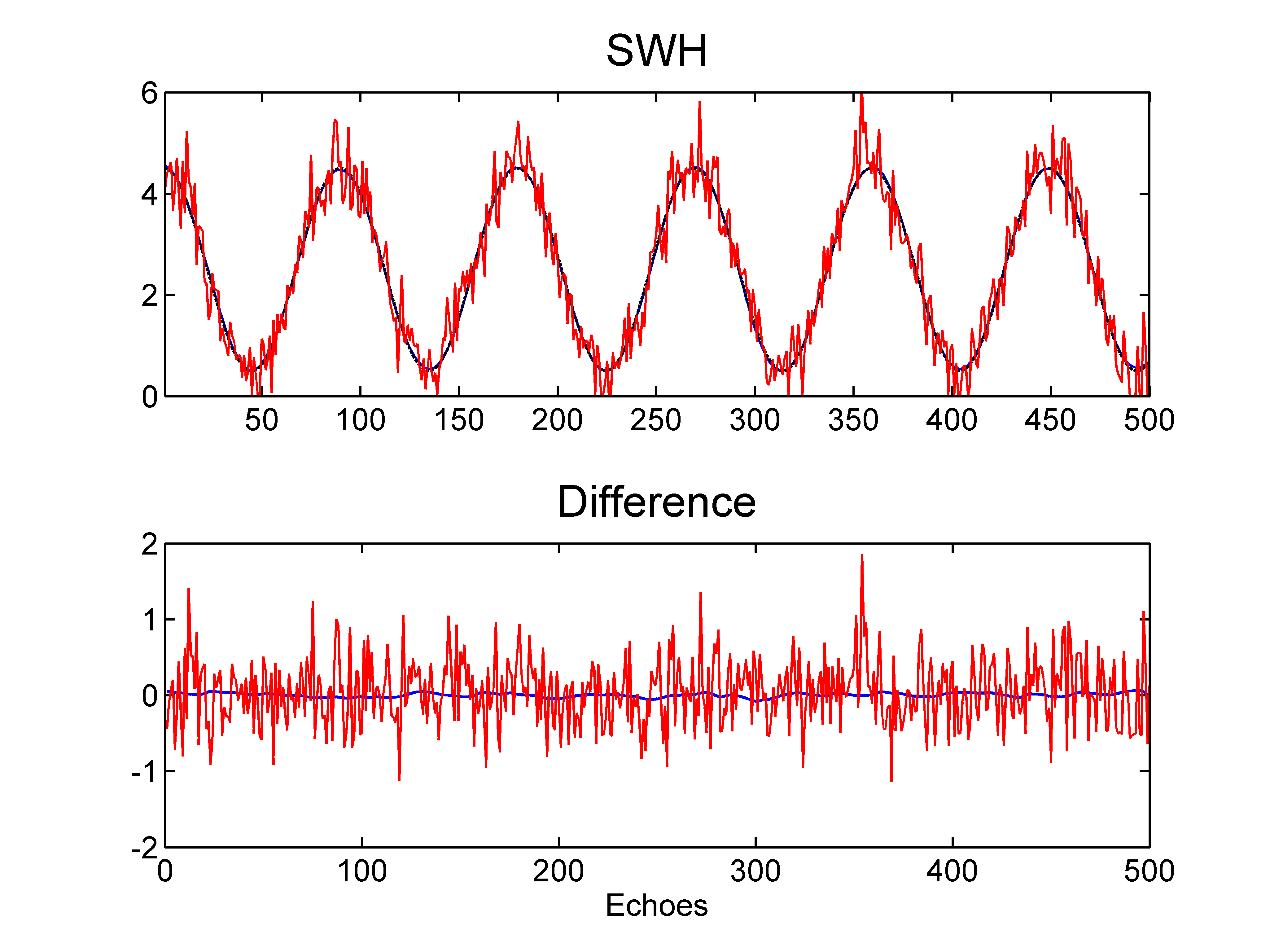
(a) SWH

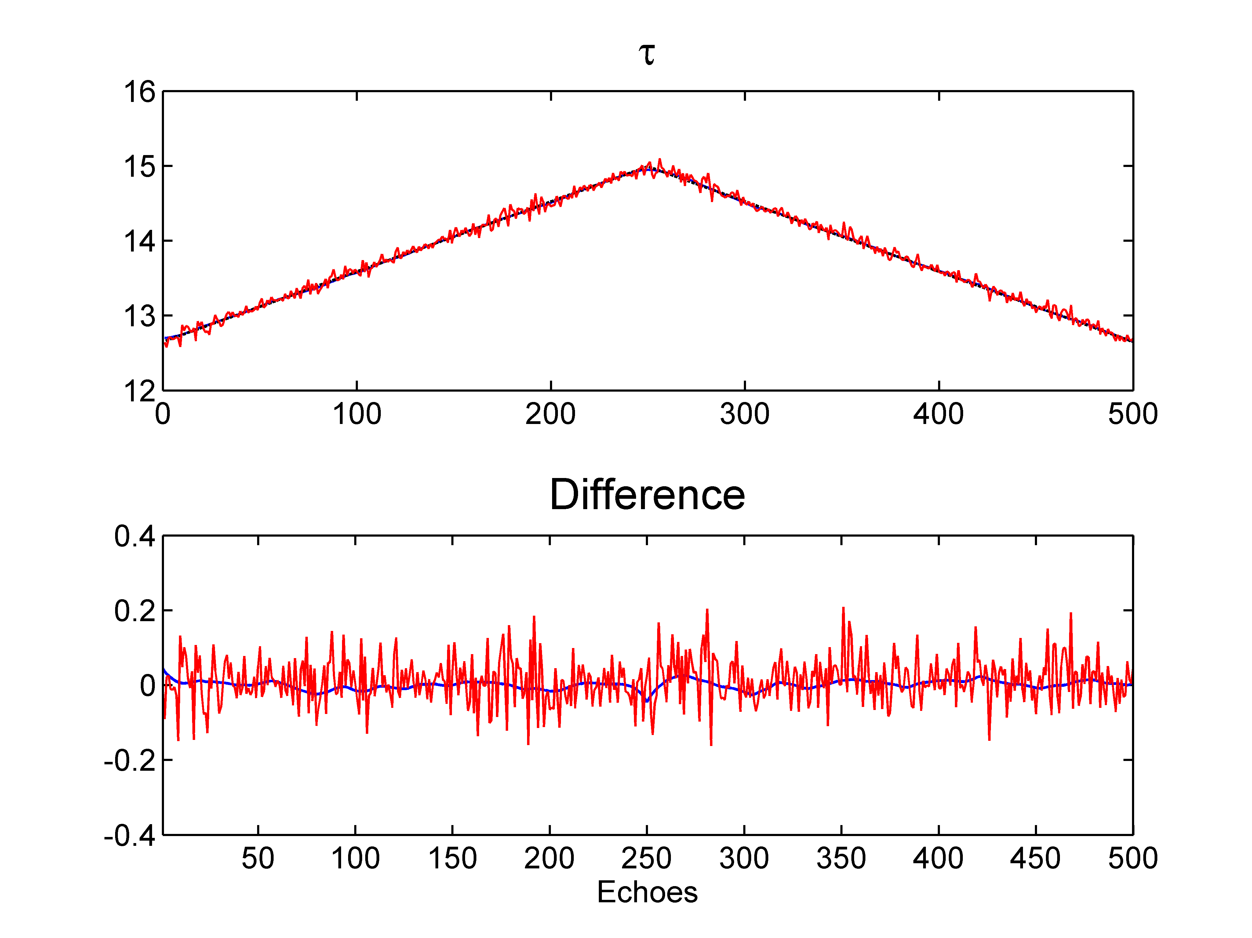
(b) $\tau$

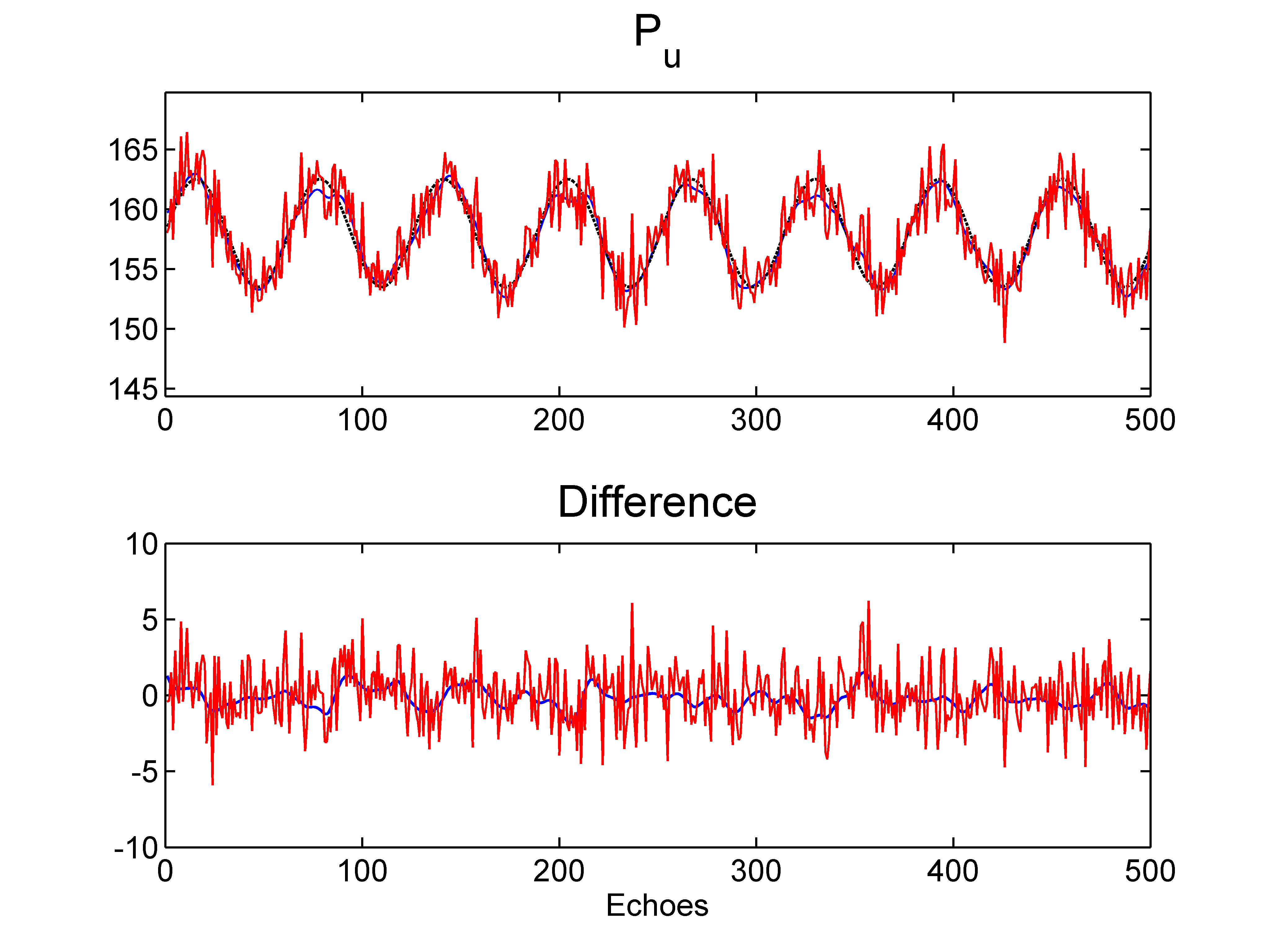
(c) $P_{u}$

Figure 2: Actual (black line) and estimated parameter using the LS algorithm (red line) and the proposed CD-BM algorithm (blue line). (a) SWH, (b) $\tau$ and (c) $P_{u}$. The bottom subfigures show the difference between the estimated and real parameters.

TABLE I: Performance on synthetic BM data ($500$ echoes).

		SWH	$\tau$	$P_{u}$	$\mu$	ENL
		(cm)	(cm)		$\times 10^{(-4)}$
Bias	LS-BM	3.18	1.1	-0.01	$0.51$	-
	CD-BM	0.32	0.08	-0.2	$0.26$	0.97
	HMC-BM	-0.02	-0.13	-0.2	$-0.1$	0.93
STD	LS-BM	44.7	6.1	1.91	$11$	-
	CD-BM	2.72	1.1	0.62	$12$	4.47
	HMC-BM	5.74	1.8	0.52	$6$	4.46
Average time	LS-BM	8.9
per echo	CD-BM	3.6
in milliseconds	HMC-BM	739.7

VI Results on real data

In order to evaluate the performance of the proposed algorithm on real data, we first present our comparison criteria. Then, two kinds of real data are considered: Jason-$2$ echoes for which BM is applied, and Cryosat-$2$ for which CA and DDA models are more appropriate.

VI-A Evaluation criteria

When processing real data, it is not possible to compare the performance of the different parameter estimation algorithms using the bias and STD defined in (37) and (38), since the true parameter values are not known. In the case of real waveforms, it is usual to compare the different parameter estimations along a pass by plotting the different obtained results [13, 9] and by considering a modified STD. The modified STD is computed using (38) in which the true parameter value is approached by the mean of the estimated parameters along $20$ successive echoes. This modified STD is called “STD at 20 Hz” [6, 36, 37].

VI-B Analysis of Jason-$2$ data with the Brown model

This section illustrates the performance of the proposed CD algorithm when applied to a real Jason-$2$ dataset. The considered data last $36$ minutes and consist of $43000$ real echoes that were extracted from the pass $30$ of cycle $35$. Figure 3 shows the parameters estimated on $700$ successive echoes along the pass when considering the LS-BM (in red), HMC-BM (in green) and CD-BM (in blue) algorithms. As observed for synthetic data in Section V, the LS-BM estimates present a high estimation noise while both CD and HMC algorithms provide smoother estimates which are physically more consistent. Moreover, CD and HMC algorithms appear to be more robust to outliers as illustrated for the estimate $\#890$ of $P_{u}$. Note that the estimated SWH is slightly larger for the Bayesian algorithms when compared to LS. This difference can be explained by the i.i.d. noise assumption used in LS algorithm which is not in adequation with the considered data as already discussed in [13, 16]. The reduction of estimation variance provided by the Bayesian algorithms is particularly noticeable when plotting the spectral power density of SWH and $\tau$ as in Fig. 4. This figure shows a clear noise reduction especially for ocean scales smaller than $100$ km for SWH and $10$ km for $\tau$ (note that we have not applied atmospheric and instrumental corrections on the estimated epoch $\tau$) which improves the observation of these scales. More quantitative results are provided in Table II. This table shows a good agreement between the means of the estimated parameters for the LS, HMC and CD algorithms (except for SWH as explained above). Bayesian algorithms also estimate the ENL which provides an indication about the noise level corrupting the data. The estimated ENL ranges between $70$ and $80$ echoes which is close to the actual value (around $90$ or $100$ echoes). As for synthetic data, the estimated STDs obtained with the CD algorithm are smaller than for LS and HMC which is of great importance for many practical applications related to oceanography such as bathymetry. Indeed, the CD algorithm improves the LS-BM STDs by a factor of about $20$ for SWH, $2$ for $\tau$ and $3$ for $P_{u}$. Note finally that the proposed CD algorithm requires a reduced computational time two times lower than that of the LS algorithm. As previously explained, this time reduction is due to the parallel scheme considered by the CD algorithm which is more efficient than the independent processing of echoes performed in the LS algorithm.

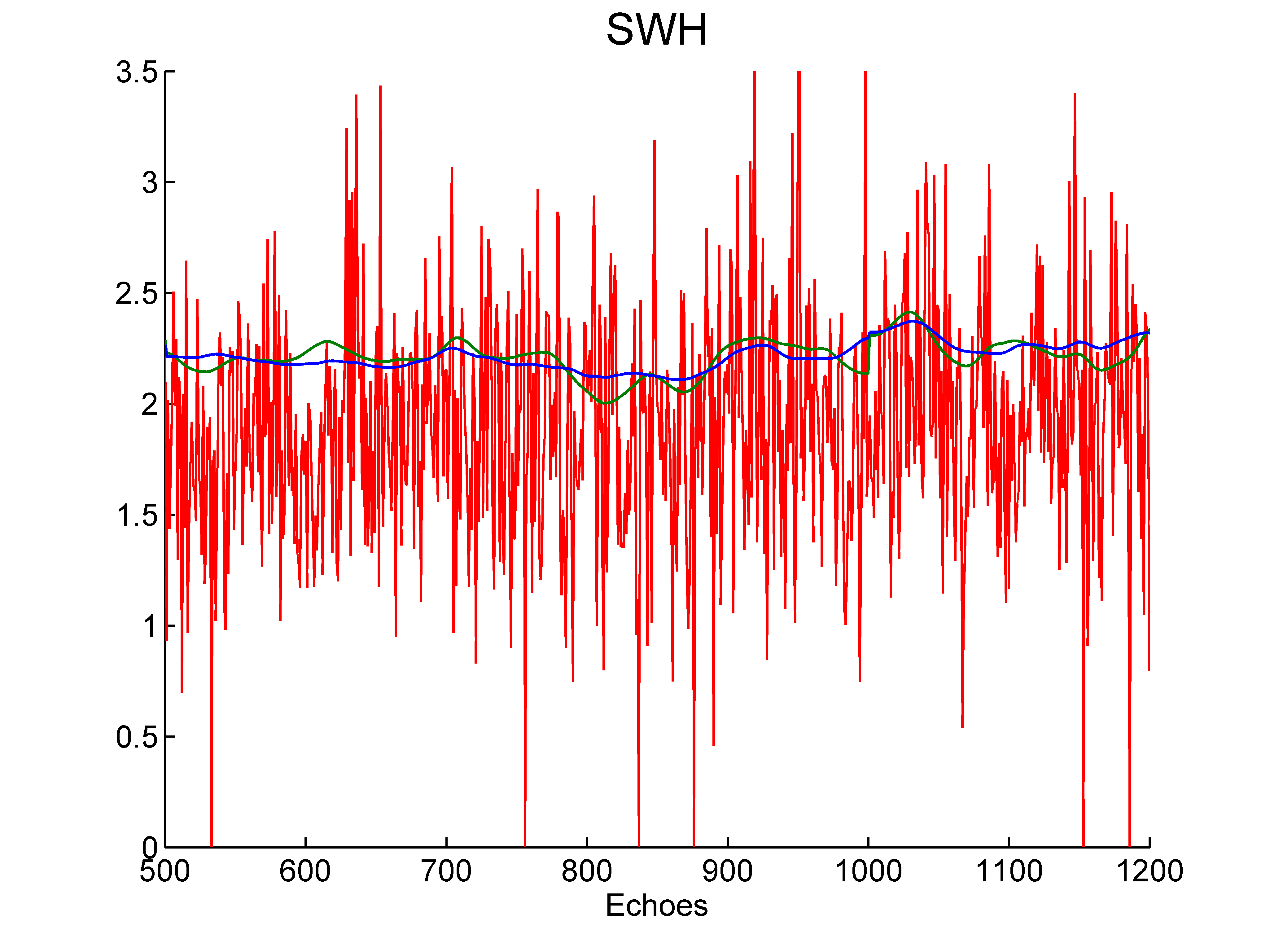
(a) SWH

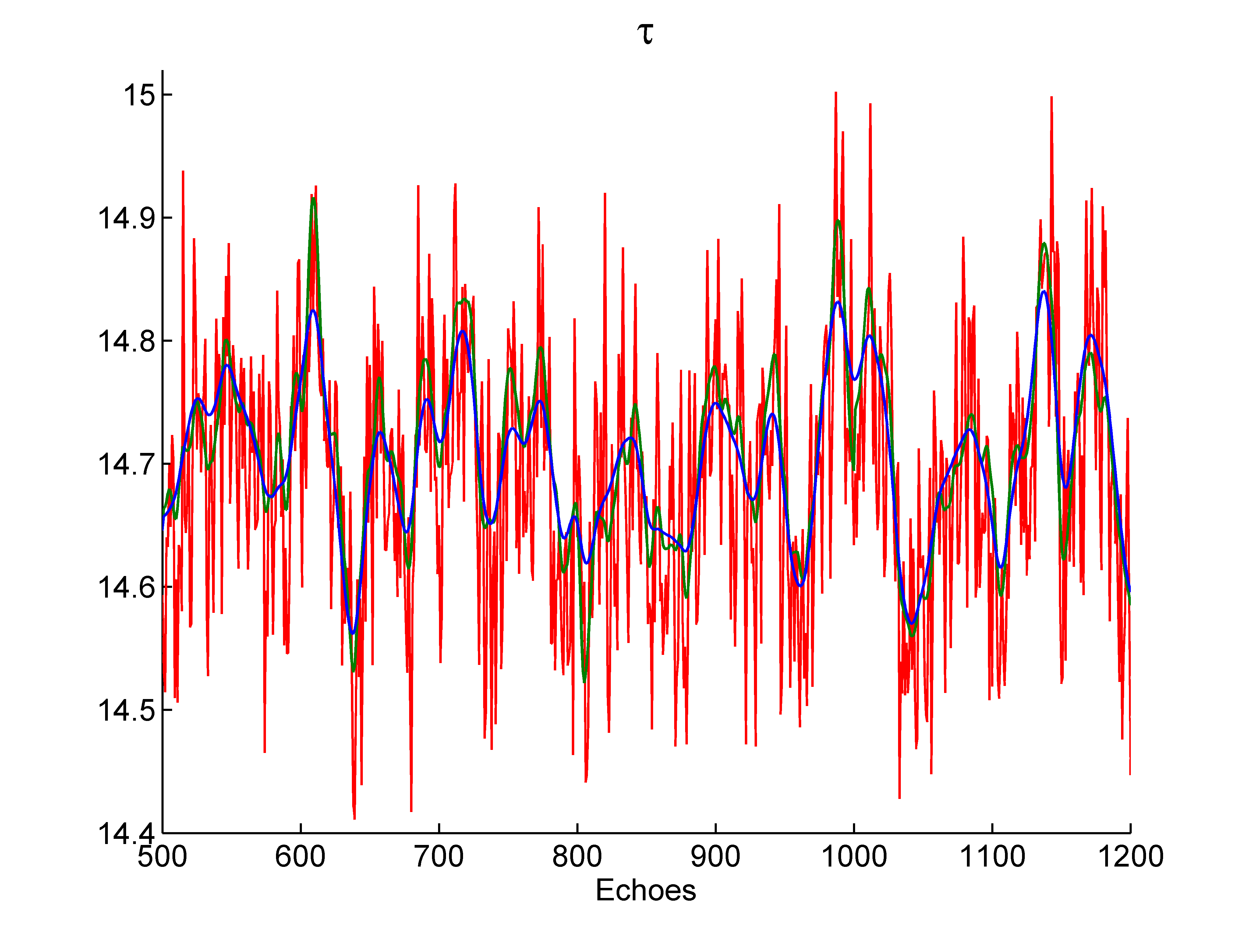
(b) $\tau$

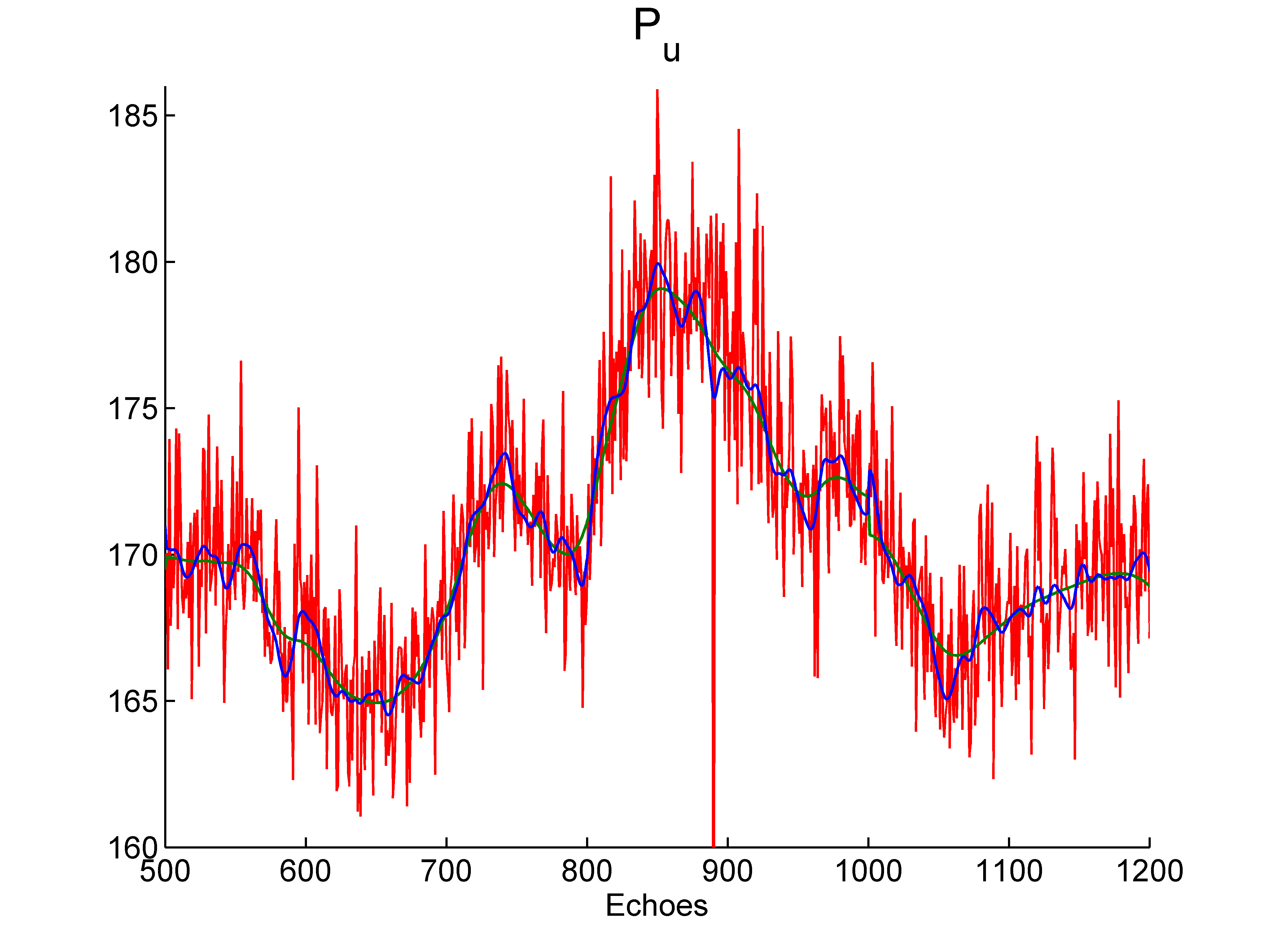
(c) $P_{u}$

Figure 3: Estimated parameters using the LS-BM algorithm (red line), the HMC-BM algorithm (green line) and the CD-BM algorithm (blue line) for Jason-$2$ echoes. (a) SWH, (b) $\tau$ and (c) $P_{u}$.

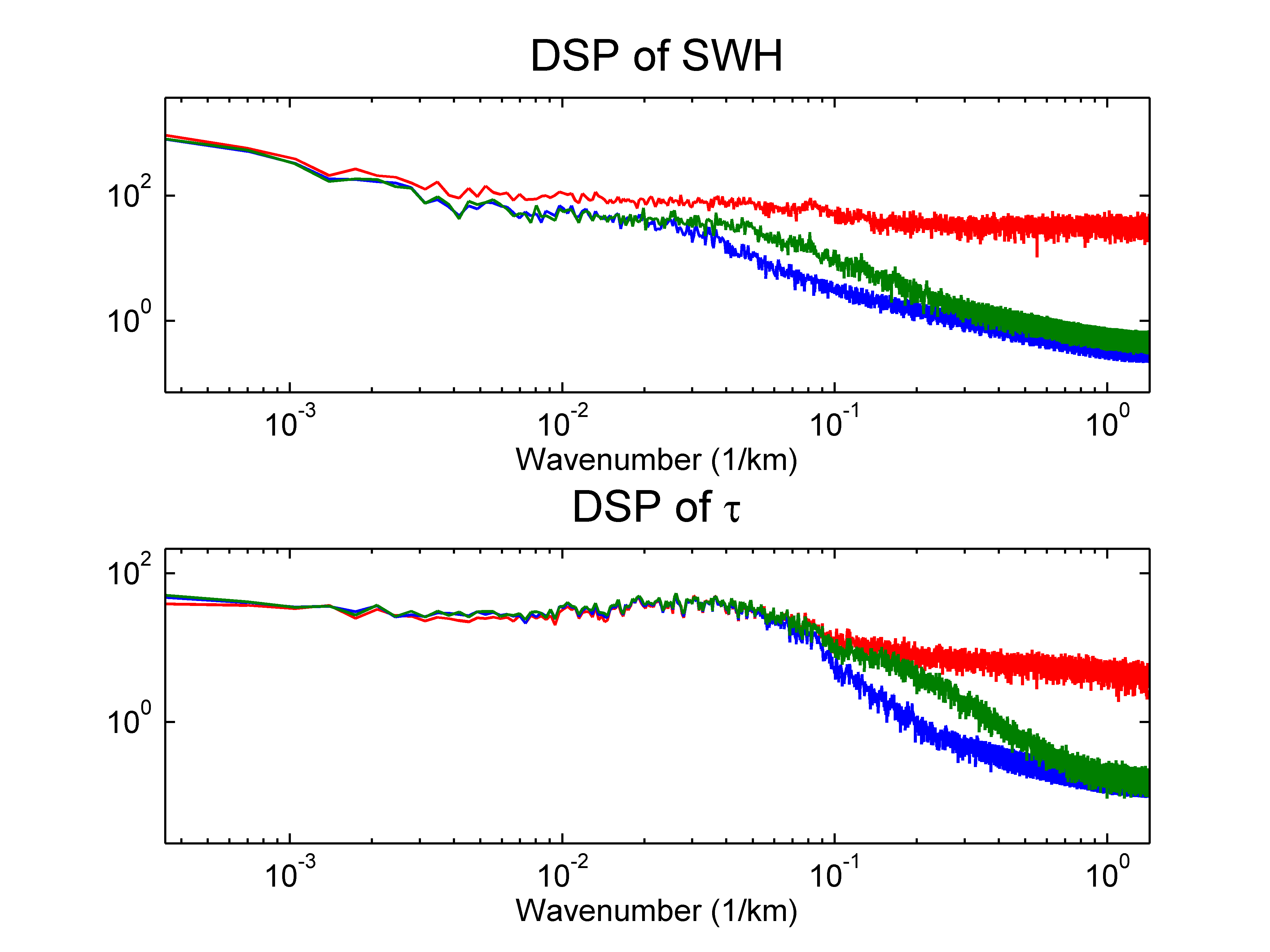
Figure 4: Estimated spectra of SWH and $\tau$ using $43000$ Jason-2 echoes with the LS algorithm (red line), the HMC-BM algorithm (green line) and the CD-BM algorithm (blue line).

TABLE II: Performance on real Jason-$2$ data ($43000$ echoes).

		SWH (cm)	$\tau$ (cm)	$P_{u}$	$\mu$	ENL
Mean	LS-BM	237	14.67	167.81	0.97	-
	CD-BM	272	14.69	167.52	1.06	74
	HMC-BM	270	14.69	167.53	1.06	80
STD	LS-BM	55.5	11.23	8.18	0.12	-
	CD-BM	2.37	5.57	2.79	0.08	15
	HMC-BM	5.58	7.11	7.64	0.08	9.5
Average time	LS-BM	12.5
per echo	CD-BM	6.6
in milliseconds	HMC-BM	1142.3

VI-C Comparison between CA and DDA for Cryosat-$2$ data

This section evaluates the performance of the proposed CD algorithm for real oceanic Cryosat-$2$ waveforms. The Cryosat-$2$ altimeter called SIRAL presents three modes that are: the low resolution mode (LRM), the synthetic aperture radar mode (SARM) and the synthetic aperture radar interferometric mode (SARInM) [38]. This paper considers data from the SARM that are used to generate CA and DDA echoes (see [6] for more details about these echoes). The considered dataset lasts approximately $100$ seconds (i.e., $2000$ echoes) and was obtained in August $2011$ by the Cryosat processing prototype (CPP) developed by CNES [41] (which is doing the level $1$ processing). Note that the CNES-CPP uses data pre-processed to full bit rate provided by ESA [38]. Table IV compares the estimated parameters using the LS algorithm with the CD and HMC algorithms when considering both CA and DDA echoes. For all algorithms, we have considered the same instrumental parameters as in [6, 7] which are given in Table III. To compare with [6], we only present the estimation results of SWH and of the sea surface height anomaly (SSHA) which represent the most important parameters (SSHA is obtained by applying all environmental corrections on the estimated epoch $\tau$). Figs. 5 and 6 show the evolution of the estimated SWH and SSHA parameters when considering the three studied algorithms. These figures show a good agreement between the estimated parameters especially between CD and HMC algorithms, which is confirmed by the mean of the estimated parameters provided in Table IV. Note that, as for Jason-$2$, a bias seems to appear between the estimated SWH parameter for Bayesian algorithms and the LS approach, which can be explained similarly. Considering the STDs, and to compare the results of Table IV with [6], one has to note that the results of [6] were obtained when using the LS algorithm for both CA and DDA. The processing of the Cryosat-$2$ data further highlights the main advantage of the proposed CD approach which is to reduce drastically the STDs of the estimated parameters. For example, STDs(SWH) (resp. STD(SSHA)) goes from $91$ cm (resp. $14$ cm) for LS-CA to $3$ cm (resp. $4$ cm) for CD-CA which represents a great improvement. The same behavior is observed when considering DDA echoes showing the interest of smoothing the altimetric parameters. The second advantage of the CD algorithm is the reduction of the computational time especially for DDA echoes. Indeed, Table IV highlights a time reduction by a factor $20$ w.r.t. LS-DDA that processed the echoes independently while CD-DDA uses a parallel scheme. For CA echoes, the CD approach shows a time improvement by a factor $1.5$ which is still an interesting result. Note finally that the HMC algorithm shows similar performance than the CD algorithm but at a price of a higher computation cost. These results confirm the good performance of the proposed algorithm and show its flexibility w.r.t. the considered altimetric models.

Parameter	Value
Frequency	$13.575$ GHz
Wavelength ($\lambda$)	$2.21$ cm
Bandwidth (B)	$320$ MHz
Altitude ($h$)	$730$ km
Burst repetition frequency (BRF)	$85$ Hz
Pulse repetition frequency (PRF)	$18182$ Hz
3 dB Antenna beam width ($\theta_{3\textrm{dB}}$)	$1.1388$ degrees
Velocity ($v_{s}$)	$7000$ m/s
Pulses per burst	$64$ pulses
Burst length ($\tau_{b}$)	$3.5$ ms
Doppler beam width	$327$ m

TABLE III: Instrumental parameters.

TABLE IV: Comparison between the LS, CD and HMC algorithms when considering real CA and DDA data    ($2000$ Cryosat-$2$ echoes).

		CA echoes			DDA echoes
		LS-CA	CD-CA	HMC-CA	LS-DDA	CD-DDA	HMC-DDA
Means	SWH (m)	2.39	2.59	2.53	2.31	2.70	2.70
	SSHA (m)	-5.12	-5.20	-5.19	-5.13	-5.20	-5.21
STDs at 20 Hz	SWH (cm)	91	3	20	45	3	8
	SSHA (cm)	14	4	4	6	2	2
Average time		0.1	0.07	252	0.79	0.04	233
per echo (s)

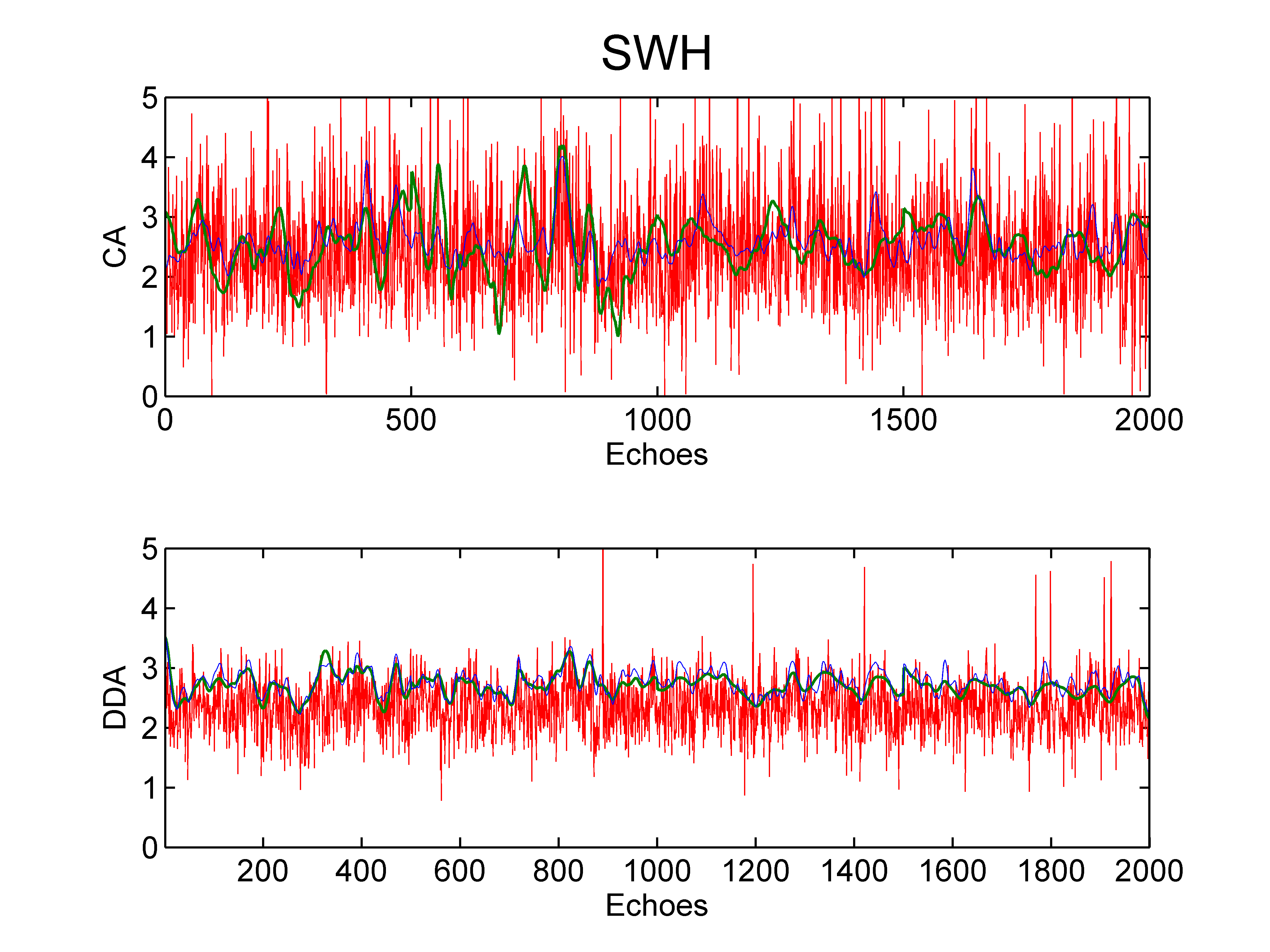
Figure 5: Estimated SWH using $2000$ Cryosat-$2$ echoes with the LS algorithm (red line), the HMC algorithm (green line) and the CD algorithm (blue line). (Top) CA echoes, (bottom) DDA echoes.

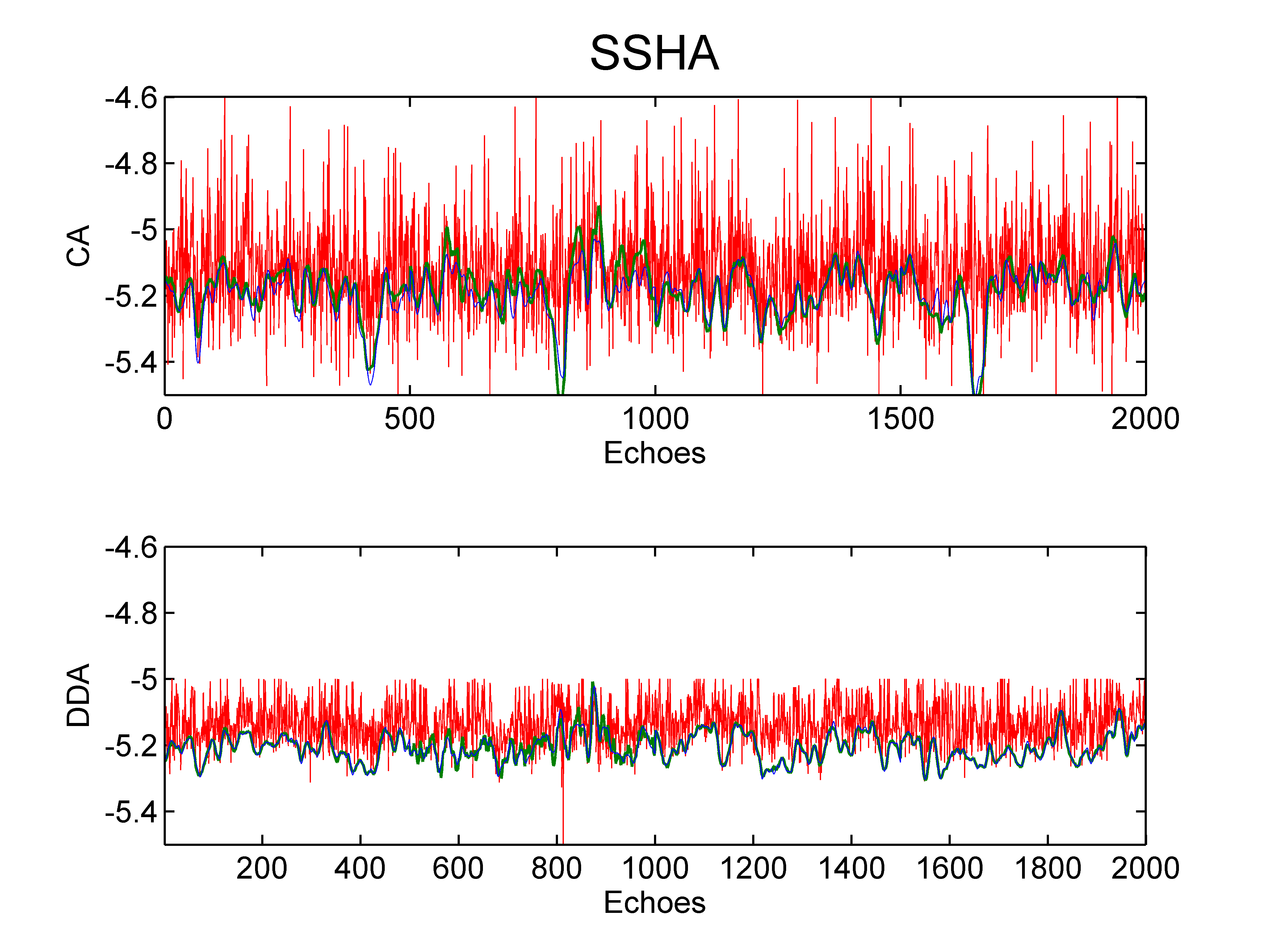
Figure 6: Estimated SSHA using $2000$ Cryosat-$2$ echoes with the LS algorithm (red line), the HMC algorithm (green line) and the CD algorithm (blue line). (Top) CA echoes, (bottom) DDA echoes.

VII Conclusions

This paper proposed a new Bayesian strategy for a smooth parameter estimation of the noise and altimetric parameters. The altimetric parameters were assigned a prior distribution enforcing a smooth temporal evolution. The altimetric signal was assumed to be corrupted by a thermal and speckle noise distributed according to an independent and non identically Gaussian distribution. The parameter estimation was achieved using a coordinate descent algorithm that presents a low computational cost which is suitable for real time applications. The proposed CD algorithm showed good performance and improved the quality of the estimated parameters when applied to both synthetic and real altimetric echoes from conventional and delay/Doppler altimetry. More precisely, it provided reduced parameter STDs and presented a lower computational cost when compared to the state-of-the-art LS algorithm. Moreover, the CD algorithm is generic and showed its efficiency when considering three altimetric models. Future work includes the consideration of other altimetric models such as the DDA-SAMOSA model [42, 43], coastal models [44, 10] and the CA model based on the true PTR [29, 30]. Considering antenna mispointing is also an interesting issue that is currently under investigation.

References

- [1] P. Vincent, N. Steunou, E. Caubet, L. Phalippou, L. Rey, E. Thouvenot, and J. Verron, “AltiKa: a Ka-band altimetry payload and system for operational altimetry during the GMES period,” Sensors, vol. 6, no. 3, pp. 208–234, Mar. 2006.
- [2] J. Richard, L. Phalippou, F. Robert, N. Stenou, E. Thouvenot, and P. Sengenes, “An advanced concept of radar altimetry over oceans with improved performances and ocean sampling : AltiKa,” in Proc. IEEE Int. Conf. Geosci. Remote Sens. (IGARSS), July 2007, pp. 3537–3540.
- [3] R. K. Raney and L. Phalippou, “The future of coastal altimetry,” in Coastal Altimetry, S. Vignudelli, A. G. Kostianoy, P. Cipollini, and J. Benveniste, Eds. Berlin: Springer Verlag, 2011, pp. 61–101.
- [4] R. K. Raney, “The delay/Doppler radar altimeter,” IEEE Trans. Geosci. Remote Sens., vol. 36, no. 5, pp. 1578–1588, Sept. 1998.
- [5] D. Wingham, L. Phalippou, C. Mavrocordatos, and D. Wallis, “The mean echo and echo cross product from a beamforming interferometric altimeter and their application to elevation measurement,” IEEE Trans. Geosci. Remote Sens., vol. 42, no. 10, pp. 2305 – 2323, Oct. 2004.
- [6] A. Halimi, C. Mailhes, J.-Y. Tourneret, P. Thibaut, and F. Boy, “A semi-analytical model for delay/Doppler altimetry and its estimation algorithm,” IEEE Trans. Geosci. Remote Sens., vol. 52, no. 7, pp. 4248–4258, July 2014.
- [7] A. Halimi, C. Mailhes, J.-Y. Tourneret, T. Moreau, and F. Boy, “Including antenna mispointing in a semi-analytical model for delay/Doppler altimetry,” IEEE Trans. Geosci. Remote Sens., vol. 53, no. 2, pp. 598–608, Feb. 2015.
- [8] G. Brown, “The average impulse response of a rough surface and its applications,” IEEE Trans. Antennas and Propagation, vol. 25, no. 1, pp. 67–74, Jan. 1977.
- [9] L. Amarouche, P. Thibaut, O. Z. Zanife, J.-P. Dumont, P. Vincent, and N. Steunou, “Improving the Jason-1 ground retracking to better account for attitude effects,” Marine Geodesy, vol. 27, no. 1-2, pp. 171–197, Aug. 2004.
- [10] A. Halimi, C. Mailhes, J.-Y. Tourneret, P. Thibaut, and F. Boy, “Parameter estimation for peaky altimetric waveforms,” IEEE Trans. Geosci. Remote Sens., vol. 51, no. 3, pp. 1568–1577, March 2013.
- [11] A. Halimi, “From conventional to delay/doppler altimetry,” Ph.D. dissertation, Institut National Polytechnique de Toulouse, Toulouse, France, 2013. [Online]. Available: http://ethesis.inp-toulouse.fr/archive/00002423/01/halimi.pdf
- [12] S. Maus, C. M. Green, and J. D. Fairhead, “Improved ocean-geoid resolution from retracked ERS-1 satellite altimeter waveforms,” vol. 134, no. 1, pp. 243–253, Feb. 1998.
- [13] D. T. Sandwell and W. H. F. Smith, “Retracking ERS-1 altimeter waveforms for optimal gravity field recovery,” Geophys. J. Int., vol. 163, no. 1, pp. 79–89, Oct. 2005.
- [14] J. Severini, C. Mailhes, J.-Y. Tourneret, and P. Thibaut, “Bayesian estimation of altimeter echo parameters,” in Proc. IEEE Int. Conf. Geosci. Remote Sens. (IGARSS), vol. 3, Boston, MA, 2008, pp. 238–241.
- [15] J.-P. Dumont, “Estimation optimale des paramètres altimétriques des signaux radar Poséidon,” Ph.D. dissertation, Institut National Polytechnique de Toulouse, Toulouse, France, 1985.
- [16] A. Halimi, C. Mailhes, and J.-Y. Tourneret, “Cramér-Rao bounds and estimation algorithms for delay/Doppler and conventional altimetry,” in Proc. EUSIPCO, Marrakech-Marocco, Sept. 9-13 2013.
- [17] C. Martin-Puig and G. Ruffini, “SAR altimeter retracker performance bound over water surfaces,” in Proc. IEEE Int. Conf. Geosci. Remote Sens. (IGARSS), Cape Town, South Africa, July 12-17, 2009, pp. 449 –452.
- [18] P. Campisi and K. Egiazarian, Blind image deconvolution: theory and applications. Boca Raton, FL: Taylor Francis, cop. 2007, 2007.
- [19] R. Molina, J. Mateos, and A. Katsaggelos, “Blind deconvolution using a variational approach to parameter, image, and blur estimation,” IEEE Trans. Image Process., vol. 15, no. 12, pp. 3715–3727, Dec. 2006.
- [20] J. Sigurdsson, M. Ulfarsson, and J. Sveinsson, “Hyperspectral unmixing with regularization,” IEEE Trans. Geosci. Remote Sens., vol. 52, no. 11, pp. 6793–6806, Nov. 2014.
- [21] L. Chaari, T. Vincent, F. Forbes, M. Dojat, and P. Ciuciu, “Fast joint detection-estimation of evoked brain activity in event-related fmri using a variational approach,” IEEE Trans. Image Processing, vol. 32, no. 5, pp. 821–837, May 2013.
- [22] A. Halimi, C. Mailhes, and J.-Y. Tourneret, “Nonlinear regression using smooth Bayesian estimation,” in Proc. IEEE Int. Conf. Acoust., Speech, and Signal Process. (ICASSP), Brisbane, Australia, April 2015, to appear.
- [23] S. Brooks, A. Gelman, G. L. . Jones, and X.-L. Meng, Handbook of Markov chain Monte Carlo. ser. Chapman Hall/CRC Handbooks of Modern Statistical Methods. Taylor Francis, 2011.
- [24] D. P. Bertsekas, Nonlinear programming. Belmont, Massachusetts: Athena Scientific, 1995.
- [25] S. Amari and S. Douglas, “Why natural gradient?” in Proc. IEEE ICASSP-98, vol. 2, May 1998, pp. 1213–1216.
- [26] P. J. Green, “Iteratively reweighted least squares for maximum likelihood estimation, and some robust and resistant alternatives,” Journal of the Royal Statistical Society. Series B (Methodological), vol. 46, no. 2, pp. 149–192, 1984.
- [27] M. Girolami and B. Calderhead., “Riemann manifold Langevin and Hamiltonian Monte Carlo methods,” Journal of the Royal Statistical Society, Series B, vol. 73, no. 2, pp. 123–214, March 2011.
- [28] M. Pereyra, H. Batatia, and S. McLaughlin, “Exploiting information geometry to improve the convergence properties of variational active contours,” Selected Topics in Signal Process., IEEE Journal of, vol. 7, no. 4, pp. 700–707, Aug. 2013.
- [29] L. Amarouche et al, “Reduction of the Sea Surface Height spectral hump using a new retracker decorrelating ocean estimated parameters (DCORE),” in Report of the Ocean Surf. Topogr. Sci. Team Meet. (OSTST), Lake Constance, Germany, Oct. 27-31, 2014.
- [30] F. Boy et al, “Towards the Jason-3 waveform processing: assessment of the numerical retracking performances,” in Report of the Ocean Surf. Topogr. Sci. Team Meet. (OSTST), Lake Constance, Germany, Oct. 27-31, 2014.
- [31] G. Hayne, “Radar altimeter mean return waveforms from near-normal-incidence ocean surface scattering,” IEEE Trans. Antennas and Propagation, vol. 28, no. 5, pp. 687–692, Sept. 1980.
- [32] L. Phalippou and F. Demeestere, “Optimal re-tracking of SAR altimeter echoes over open ocean: from theory to results for SIRAL2,” in Report of the Ocean Surf. Topogr. Sci. Team Meet. (OSTST), San Diego, California, Oct. 19-21, 2011. [Online]. Available: http://www.aviso.oceanobs.com/fileadmin/documents/OSTST/2011/oral/01˙Wednesday/Splinter%201%20IP/02%20OSTST-2011-Phalippou-Demeestere.pdf
- [33] O. Germain and G. Ruffini, “A revisit to the GNSS-R code range precision,” in Proc. GNSS-R, Noordwijk, The Netherlands, June 14-15, 2006.
- [34] C. Martin-Puig, P. Berry, R. Smith, C. Gommenginger, G. Ruffini, P. Cipollini, L. Stenseng, A. O., P. Cotton, J. Benveniste, and S. Dinardo, “SAR altimetry over water surfaces,” in Oceans from Space, Venice, Italy, April 2010.
- [35] V. Mazet, “Joint bayesian decomposition of a spectroscopic signal sequence,” IEEE Signal Processing Lett., vol. 18, no. 3, pp. 181–184, March 2011.
- [36] K. Giles, D. Wingham, N. Galin, R. Cullen, and W. Smith, “Precise estimates of ocean surface parameters from cryosat,” in Report of the Ocean Surf. Topogr. Sci. Team Meet. (OSTST), Venice-Lido, Italy, Sept. 22-29, 2012. [Online]. Available: http://www.aviso.oceanobs.com/fileadmin/documents/OSTST/2012/oral/02˙friday˙28/05˙instr˙processing˙IIb/02˙IP2B˙Giles.pdf
- [37] C. Gommenginger, C. Martin-Puig, S. Dinardo, D. Cotton, M. Srokosz, and J. Benveniste, “Improved altimetric accuracy of SAR altimeters over the ocean: observational evidence from Cryosat-2 SAR and Jason-2,” in Report of the Ocean Surf. Topogr. Sci. Team Meet. (OSTST), San Diego, California, Oct. 19-21, 2011. [Online]. Available: http://www.aviso.oceanobs.com/fileadmin/documents/OSTST/2011/oral/01˙Wednesday/Splinter%201%20IP/01%20Gommenginger%20SAMOSA˙OSTST˙Oct2011.pdf
- [38] D. Wingham, C. R. Francis, S. Baker, C. Bouzinac, D. Brockley, R. Cullen, P. de Chateau-Thierry, S. Laxon, U. Mallow, C. Mavrocordatos, L. Phalippou, G. Ratier, L. Rey, F. Rostan, P. Viau, and D. Wallis, “Cryosat: A mission to determine the fluctuations in Earth’s land and marine ice fields,” vol. 37, no. 4, pp. 841 – 871, July 2006.
- [39] W. H. F. Smith and R. Scharroo, “Pulse-to-pulse correlation in Cryosat SAR echoes from ocean surfaces: implications for optimal pseudo-LRM waveform averaging,” in Report of the Ocean Surf. Topogr. Sci. Team Meet. (OSTST), Venice-Lido, Italy, Sept. 22-29, 2012. [Online]. Available: http://www.aviso.oceanobs.com/fileadmin/documents/OSTST/2012/oral/02˙friday˙28/05˙instr˙processing˙IIb/03˙IP2B˙Smith1.pdf
- [40] C. Gommenginger, P. Cipollini, D. Cotton, S. Dinardo, and J. Benveniste, “Finer, better, closer: Advanced capabilities of SAR altimetry in the open ocean and the coastal zone,” in Report of the Ocean Surf. Topogr. Sci. Team Meet. (OSTST), Venice-Lido, Italy, Sept. 22-29, 2012. [Online]. Available: http://www.aviso.oceanobs.com/fileadmin/documents/OSTST/2012/oral/02˙friday˙28/02˙instr˙processing˙II/01˙IP2˙Gommenginger.pdf
- [41] F. Boy, J.-D. Desjonqueres, A. Halimi, P. Thibaut, T. Moreau, and N. Picot, “Cryosat Processing Prototype, LRM and SAR processing on CNES side and a comparison to DUACS SLA,” in Report of the Ocean Surf. Topogr. Sci. Team Meet. (OSTST), Venice-Lido, Italy, Sept. 22-29, 2012. [Online]. Available: http://www.aviso.oceanobs.com/fileadmin/documents/OSTST/2012/oral/02˙friday˙28/02˙instr˙processing˙II/02˙IP2˙Boy.pdf
- [42] C. Martin-Puig, G. Ruffini, J. Marquez, D. Cotton, M. Srokosz, P. Challenor, R. K. Raney, and J. Benveniste, “Theoretical model of SAR altimeter over water surfaces,” in Proc. IEEE Int. Conf. Geosci. Remote Sens. (IGARSS), Boston, U.S.A., July 7-11, 2008, pp. 242 – 245.
- [43] C. Gommenginger, C. Martin-Puig, S. Dinardo, D. Cotton, and J. Benveniste, “Improved altimetric performance of Cryosat-2 SAR mode over the open ocean and the coastal zone,” in Proc. IEEE Int. Conf. Geosci. Remote Sens. (IGARSS), Munich, Germany, July 22-27, 2012.
- [44] J. Gómez-Enri, S. Vignudelli, G. D. Quartly, C. P. Gommenginger, P. Cipollini, P. G. Challenor, and J. Benveniste, “Modeling ENVISAT RA-2 waveforms in the coastal zone: Case study of calm water contamination,” IEEE Geosci. Remote Sens. Lett., vol. 7, no. 3, pp. 474–478, July 2010.
- [45] C. P. Robert, The Bayesian Choice: from Decision-Theoretic Motivations to Computational Implementation, 2nd ed., ser. Springer Texts in Statistics. New York: Springer-Verlag, 2007.
- [46] A. Halimi, N. Dobigeon, and J.-Y. Tourneret, “Unsupervised unmixing of hyperspectral images accounting for endmember variability,” in ArXiv e-prints, Jun. 2014.