Gamow-Teller response and its spreading mechanism in doubly magic nuclei

Abstract

The scope of the paper is to apply a state-of-the-art beyond mean-field model to the description of the Gamow-Teller response in atomic nuclei. This topic recently attracted considerable renewed interest, due, in particular, to the possibility of performing experiments in unstable nuclei. We study the cases of ⁴⁸Ca, ⁷⁸Ni, ¹³²Sn and ²⁰⁸Pb. Our model is based on a fully self-consistent Skyrme Hartree-Fock plus random phase approximation. The same Skyrme interaction is used to calculate the coupling between particles and vibrations, which leads to the mixing of the Gamow-Teller resonance with a set of doorway states and to its fragmentation. We compare our results with available experimental data. The microscopic coupling mechanism is also discussed in some detail.

today

I Introduction

Spin-isospin resonances are not a new subject, yet they still capture the interest of researchers, both experimentalists and theorists, not only in nuclear physics but also in particle physics and astrophysics. There exist some review papers Osterfeld (1992); Ichimura et al. (2006), that do not cover, however, the most recent developments. From the experimental point of view, the forefront of such kind of research is the exploration of the spin-isospin modes in exotic nuclei (mainly neutron-rich and possibly drip-line isotopes). This is nowadays possible due to the advent of radioactive beam facilities, and a dedicated effort focused on charge-exchange reactions leading to spin-isospin modes is ongoing, e.g., in Japan and in the USA. The Gamow-Teller (GT) excitations are the main goal but spin-dipole or other multipoles are also of interest.

Effective nucleon-nucleon forces are poorly constrained in the spin-isospin channel, and they often display unphysical ferromagnetic instabilities in nuclear matter at high densities that need to be cured (cf. Navarro and Polls (2013); Chamel and Goriely (2010) and references therein). A systematic exploration of spin-isospin transitions, from light to medium-heavy systems and from the neutron-deficient to the neutron-rich side, is needed, in order to tune such effective nucleon-nucleon interactions in the nuclear medium and to study the nuclear equation of state. It has been shown, for instance, that the spin-dipole strength is a good indicator of the neutron skin (cf. Colò et al. (2014) and references therein). Most of the GT strength in the $t_{-}$ channel lies at high excitation energy in stable nuclei; however, as the neutron excess increases, one expects that a sizable part of it can move down into the $\beta$-decay window Sagawa et al. (1993). To what extent this happens, and/or brings new information on the spin-isospin part of the nuclear Hamiltonian, is still an open question: although it can be at present mainly tackled in light nuclei such as ⁸He Kobayashi et al. (2014) and ¹²Be, there are attempts towards the neutron-rich side in heavy systems as well (for instance, in the case of ¹³²Sn).

Spin-isospin excitations play an important role in the weak-interaction processes such as electron capture, $\beta$ decay, and neutrino-nucleus reactions. Therefore, the knowledge of selected transitions in a specific series of nuclei, or in specific regions of the nuclear chart, is of great interest for nuclear astrophysics Langanke and Martínez-Pinedo (2003); Janka et al. (2007). A clear and well-known example is that of core-collapse supernovae. In this case, the electron capture rates govern the evolution of the system and consequently, GT transition matrix elements must be accurately known in the iron region Langanke and Martínez-Pinedo (2003); Janka et al. (2007); Paar et al. (2009); Niu et al. (2011); Fantina et al. (2012). The $\beta$-decay half-lives set the time scale of the rapid neutron capture process ($r$ process), and hence influence the production of heavy elements in the universe Burbidge et al. (1957); Qian and Wasserburg (2007); Niu et al. (2013). Last but not least, a very accurate knowledge of spin-isospin matrix elements is also instrumental to extract the properties of the neutrinos from the measured half-life of double-$\beta$ decay Avignone et al. (2008); Vergados et al. (2012).

From the theoretical point of view, in the last two decades there has been significant progress in microscopic models aimed at the description of collective excitations such as the charge-exchange GT and spin-dipole resonances. Most nuclei in the nuclear chart can be studied by models based on self-consistent mean-field or density functional theory. At present, they can be employed in the form of a Hartree [or Hartree-Fock (HF)] approximation for the ground-state plus charge-exchange random phase approximation (RPA) to determine the main resonance properties. This can be done using Skyrme Auerbach and Klein (1984); Hamamoto and Sagawa (2000); Bender et al. (2002); Fracasso and Colò (2007); Bai et al. (2009a); Roca-Maza et al. (2012) or Gogny Martini et al. (2014) effective Hamiltonians, as well as using covariant effective Lagrangians De Conti et al. (2000); Paar et al. (2004); Liang et al. (2008). Some of these Hamiltonians or Lagrangians can reproduce the experimentally observed mean energy, and the fraction of the exhausted sum rule, for the GT and spin-dipole resonances, although they are not based on the same physical picture.

Self-consistent mean-field models have also limitations. It is well known that they cannot account for the spreading widths of giant resonances. The problem of the fragmentation of the GT strength has been addressed using second RPA Drożdż et al. (1990) and the quasiparticle-phonon model Kuzmin and Soloviev (1984) (see also Ref. Dang et al. (1997)). Generally speaking, models based on particle-vibration coupling (PVC) are quite effective in reproducing the giant resonance widths Bertsch et al. (1983). We apply such an approach in the present paper, which is a follow-up of Ref. Niu et al. (2012). As described in that work, some of us implemented a scheme based on the fully self-consistent Skyrme HF plus RPA, in which specific diagrams associated with PVC corrections at lowest order are introduced, and no further approximation has been done. In particular, the same Skyrme force is used to calculate the single-particle levels and the RPA spectrum (including both the GT state and the low-lying surface vibrations to be coupled to it), as well as the PVC vertices (see next section). While the model is similar to the one of Ref. Colò et al. (1994), it includes many improvements; in particular, all the terms of the Skyrme interaction are taken into account. Our goal here is to see if we can reproduce the line shape of the strength function, and the associated spreading width, observed in different nuclei and in different mass regions. In particular, we wish to make predictions for exotic nuclei for which experiments have already been carried out and not yet analyzed, or are planned. We share part of our motivations with the recent work of Ref. Litvinova et al. (2014) which adopts a model similar to ours, but based on a covariant description. We also present a detailed discussion of the spreading mechanism within our approach. The damping width of giant resonances has also a contribution coming from the escape width; that is, from the nucleon emission. In the GTR case, experiment indicates that the escape width is very small (of the order of $\approx$4% of the total width in ²⁰⁸Pb, cf. Table 8.3 of Harakeh and van der Woude (2001)). Consequently, we have not included the continuum coupling in the present paper, and we compare directly the calculated spreading width with the total experimental width.

The outline of our work is as follows. In Sec. II a short account of the formalism is presented. In Sec. III.1 the GT strength distributions and cumulative sums calculated for nuclei ²⁰⁸Pb, and ⁴⁸Ca are compared with the experimental data, while predictions are provided for ¹³²Sn and ⁷⁸Ni. The overall features of the GT resonance (GTR) and phonons are summarized in Sec. III.2. The PVC mechanism for the spreading and fragmentation of GTR is discussed in Sec. III.3. Finally, the main conclusions of this work are summarized in Sec. IV.

II Formalism

We employ the same formalism as in Ref. Niu et al. (2012), and here we only recall its essential points. We first carry out a self-consistent HF+RPA calculation of the GT strength, using a standard Skyrme interaction. The HF equations are solved in coordinate space on a radial mesh of size $0.1$ fm, within a spherical box having a radius equal to $21$ fm. The continuum is discretized by requiring vanishing boundary conditions for the wave functions at the edge of this box. A set of RPA eigenstates $|n\rangle$ for the GT excitations are obtained by the diagonalization of the RPA matrix. Forward-going and backward-going amplitudes associated with the RPA eigenstates $|n\rangle$ will be denoted by $X^{(n)}_{ph}$ and $Y^{(n)}_{ph}$, respectively. Single-particle states up to 100 MeV have been included in the particle-hole (p-h) configuration space. Within PVC, the RPA strength will be shifted and redistributed through the coupling to a set of doorway states, denoted by $|N\rangle$, made of a p-h excitation coupled to a collective vibration of angular momentum $L$. The properties of these collective vibrations, i.e., phonons $|nL\rangle$ are, in turn, obtained by computing the RPA response with the same Skyrme interaction, for states of natural parity $L^{\pi}=0^{+}$, $1^{-}$, $2^{+}$, $3^{-}$, $4^{+}$, $5^{-}$, and $6^{+}$. For the PVC model space, we have retained the phonons with energy less than 20 MeV and absorbing a fraction of the total isoscalar or isovector strength larger than $5\%$, and included intermediate particle states up to an energy of 100 MeV.

The GT strength associated with RPA+PVC, is given by

$$S(\omega)=-\frac{1}{\pi}{\rm Im}\sum_{\nu}\langle 0|\hat{O}_{\rm GT^{\pm}}|\nu\rangle^{2}\frac{1}{\omega-\Omega_{\nu}+i(\frac{\Gamma_{\nu}}{2}+\Delta)},$$ (1)

where the GT operator is $\hat{O}_{\rm GT^{\pm}}=\sum_{i=1}^{A}\mathbf{\sigma}(i)\tau_{\pm}(i)$. In our calculation, we will only focus on the GT^- excitations. $|\nu\rangle$ denote the eigenstates [associated with the complex eigenvalues $\Omega_{\nu}-i\frac{\Gamma_{\nu}}{2}$ and eigenvectors $(F^{(\nu)},\bar{F}^{(\nu)})$] that are obtained by diagonalizing the energy-dependent complex matrix

$$\left(\begin{array}[]{cc}{\cal D}+{\cal A}_{1}(\omega)&{\cal A}_{2}(\omega)\\ -{\cal A}_{3}(\omega)&-{\cal D}-{\cal A}_{4}(\omega)\end{array}\right)\left(\begin{array}[]{c}F^{(\nu)}\\ \bar{F}^{(\nu)}\end{array}\right)=(\Omega_{\nu}-i\frac{\Gamma_{\nu}}{2})\left(\begin{array}[]{c}F^{(\nu)}\\ \bar{F}^{(\nu)}\end{array}\right).$$ (2)

Here, ${\cal D}$ is a diagonal matrix containing the positive RPA eigenvalues, and the ${\cal A}_{i}$ matrices are associated with the coupling to the doorway states. The expressions of ${\cal A}_{i}$ in the RPA basis $|n\rangle$ are given by

$$({\cal A}_{1})_{mn} = \sum_{ph,p^{\prime}h^{\prime}}W^{\downarrow}_{ph,p^{\prime}h^{\prime}}(\omega)X_{ph}^{(m)}X^{(n)}_{p^{\prime}h^{\prime}}+W^{\downarrow*}_{ph,p^{\prime}h^{\prime}}(-\omega)Y_{ph}^{(m)}Y^{(n)}_{p^{\prime}h^{\prime}},$$ (3)

$$({\cal A}_{2})_{mn} = \sum_{ph,p^{\prime}h^{\prime}}W^{\downarrow}_{ph,p^{\prime}h^{\prime}}(\omega)X_{ph}^{(m)}Y^{(n)}_{p^{\prime}h^{\prime}}+W^{\downarrow*}_{ph,p^{\prime}h^{\prime}}(-\omega)Y_{ph}^{(m)}X^{(n)}_{p^{\prime}h^{\prime}},$$ (4)

$$({\cal A}_{3})_{mn} = \sum_{ph,p^{\prime}h^{\prime}}W^{\downarrow}_{ph,p^{\prime}h^{\prime}}(\omega)Y_{ph}^{(m)}X^{(n)}_{p^{\prime}h^{\prime}}+W^{\downarrow*}_{ph,p^{\prime}h^{\prime}}(-\omega)X_{ph}^{(m)}Y^{(n)}_{p^{\prime}h^{\prime}},$$ (5)

$$({\cal A}_{4})_{mn} = \sum_{ph,p^{\prime}h^{\prime}}W^{\downarrow}_{ph,p^{\prime}h^{\prime}}(\omega)Y_{ph}^{(m)}Y^{(n)}_{p^{\prime}h^{\prime}}+W^{\downarrow*}_{ph,p^{\prime}h^{\prime}}(-\omega)X_{ph}^{(m)}X^{(n)}_{p^{\prime}h^{\prime}},$$ (6)

where $W^{\downarrow}$ reads

$$W^{\downarrow}_{ph,p^{\prime}h^{\prime}}(\omega)=\sum_{N}\frac{\langle ph|V|N\rangle\langle N|V|p^{\prime}h^{\prime}\rangle}{\omega-\omega_{N}}.$$ (7)

The matrix elements are given by the sum of the four Feynman diagrams represented in Fig. 1, whose analytic expressions are

$$W^{\downarrow}_{1php^{\prime}h^{\prime}} = \delta_{hh^{\prime}}\delta_{j_{p}j_{p^{\prime}}}\sum_{p^{\prime\prime},nL}\frac{1}{\omega-(\omega_{nL}+\epsilon_{p^{\prime\prime}}-\epsilon_{h})+i\Delta}\frac{\langle p||V||p^{\prime\prime},nL\rangle\langle p^{\prime}||V||p^{\prime\prime},nL\rangle}{\hat{j}_{p}^{2}},$$

$$W^{\downarrow}_{2php^{\prime}h^{\prime}} = \delta_{p{p^{\prime}}}\delta_{j_{h}j_{h^{\prime}}}\sum_{h^{\prime\prime},nL}\frac{1}{\omega-(\omega_{nL}-\epsilon_{h^{\prime\prime}}+\epsilon_{p})+i\Delta}\frac{\langle h^{\prime\prime}||V||h,nL\rangle\langle h^{\prime\prime}||V||h^{\prime},nL\rangle}{\hat{j}_{h}^{2}},$$

$$W^{\downarrow}_{3php^{\prime}h^{\prime}} = \sum_{nL}\frac{(-)^{j_{p}-j_{h^{\prime}}+J+L}}{\omega-(\omega_{nL}+\epsilon_{p}-\epsilon_{h^{\prime}})+i\Delta}\left\{\begin{array}[]{ccc}j_{p}&j_{h}&J\\ j_{h^{\prime}}&j_{p^{\prime}}&L\end{array}\right\}\langle p^{\prime}||V||p,nL\rangle\langle h^{\prime}||V||h,nL\rangle,$$ (10)

$$W^{\downarrow}_{4php^{\prime}h^{\prime}} = \sum_{nL}\frac{(-)^{j_{p^{\prime}}-j_{h}+J+L}}{\omega-(\omega_{nL}+\epsilon_{p^{\prime}}-\epsilon_{h})+i\Delta}\left\{\begin{array}[]{ccc}j_{p}&j_{h}&J\\ j_{h^{\prime}}&j_{p^{\prime}}&L\end{array}\right\}\langle p||V||p^{\prime},nL\rangle\langle h||V||h^{\prime},nL\rangle.$$ (13)

In the above formulas, $p$ and $h$ label particle and hole states, respectively. The corresponding angular momentum and single-particle energies are given respectively by $j_{p}$, $j_{h}$ and $\epsilon_{p}$, $\epsilon_{h}$. ${\hat{j}_{i}^{2}}$ is a shorthand notation for $2j_{i}+1$, while $\omega_{nL}$ denotes the energy of the phonon state $|nL\rangle$. The averaging parameter $\Delta$ is introduced to avoid singularities in the denominator of Eq. (II), and a convenient practical value is $\Delta=200$ keV. Such a value is usually smaller than $\Gamma_{\nu}/2$ and does not affect appreciably the RPA+PVC calculation of the strength in Eq. (1) (it was in fact neglected in the calculations of the strength in Ref. Niu et al. (2012)). In the following, we shall also show calculations with larger values of $\Delta$, in order to simulate the experimental resolution. A larger value of $\Delta$ can also effectively take into account the coupling to more complex configurations not included in the current model.

Figure 1: Diagrammatic representation of the four terms whose sum gives the matrix element $W^{\downarrow}_{ph,p^{\prime}h^{\prime}}$. The analytic expressions are shown in Eq. (II).

A useful approximation to the full diagonalization of the matrix in Eq. (2) can be obtained by retaining only the diagonal term $({\cal A}_{1})_{mm}$, which is defined as self-energy $\Sigma_{m}$. If only a single pronounced GTR peak having energy $E_{\rm RPA}$ and strength $|\langle 0|\hat{O}_{\rm GT^{-}}|\rm GTR\rangle|^{2}$ from the RPA calculation is considered, one obtains the following approximate expression for the strength of Eq. (1)

$$S(\omega)=\frac{1}{\pi}\frac{\frac{\Gamma_{\rm GTR}(\omega)}{2}+\Delta}{[\omega-\Omega_{\rm GTR}(\omega)]^{2}+(\frac{\Gamma_{\rm GTR}(\omega)}{2}+\Delta^{2})}|\langle 0|\hat{O}_{\rm GT^{-}}|{\rm GTR}\rangle|^{2},$$ (15)

where

$$\Omega_{\rm GTR}(\omega)=E_{\rm RPA}+{\rm Re}[({\cal A}_{1})_{\rm GTR,GTR}(\omega)]$$ (16)

and

$$\Gamma_{\rm GTR}(\omega)=-2{\rm Im}[({\cal A}_{1})_{\rm GTR,GTR}(\omega)].$$ (17)

A simple perturbative expression for the strength function Eq. (15) can be obtained by putting $\omega=E_{\rm RPA}$ in Eqs. (16) and (17). However, a much better approximation can be obtained by solving Eq. (16) with $\Omega_{\rm GTR}(\omega)=\omega$ self-consistently. The effectiveness and usefulness of these approximations will be further discussed in Sec. III.3.

III Results and Discussions

III.1 Gamow-Teller strength distributions and cumulative sums

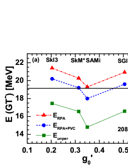
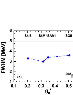
Figure 2: (Color online) Gamow-Teller resonance peak energy [panel (a)] and FWHM [panel (b)] in ²⁰⁸Pb, calculated within HF (squares), RPA (triangles), and RPA+PVC (circles) approaches with the Skyrme interactions SkI3, SkM*, SAMi, and SGII. For convenience, they are shown as a function of the Landau parameter $g_{0}^{\prime}$ associated with each force. The unperturbed HF energy $E_{\rm unper}$ is the weighted average of the two main configurations $\nu i_{13/2}\rightarrow\pi i_{11/2}$ and $\nu h_{11/2}\rightarrow\pi h_{9/2}$. The experimental peak energy and width are shown by the black straight lines.

Our calculations can be performed using different Skyrme parameter sets. Consequently, before discussing in detail the results for the GT strength functions in a series of nuclei, some considerations about the interaction dependence are in order. We display in Fig. 2 the GTR peak energy calculated in ²⁰⁸Pb within the HF, RPA, and RPA+PVC approaches, as well as the GTR full width at half maximum (FWHM) calculated within the RPA+PVC approach, with the Skyrme forces SkI3 Reinhard and Flocard (1995), SkM* Bartel et al. (1982), SAMi Roca-Maza et al. (2012) and SGII Van Giai and Sagawa (1981), as a function of the Landau parameter $g_{0}^{\prime}$ associated with each force, and using the value $\Delta=$ 1 MeV for the averaging parameter. The black straight line in the left panel denotes the experimental peak energy with respect to the parent nucleus (19.2 MeV), while the experimental width (5 MeV) is represented in the same way in the right panel. As is well known, the unperturbed HF peaks underestimate the peak energy by several MeV. The residual interaction included in the RPA calculation raises these values by 4-5 MeV, overestimating the experimental energy by $\approx$ 1-2 MeV, except for the interaction SAMi Roca-Maza et al. (2012), a newly proposed interaction with a good description of the nuclear spin-isospin properties, that was fitted so as to reproduce the experimental value at RPA level. The inclusion of PVC acts in a similar way in the four cases. The peak energies are shifted down by about 1.2 MeV and acquire a width. The FWHM is equal to $\approx$ 3.5 MeV. More precisely, the smallest effect from PVC (1.1 MeV energy shift and 3 MeV FWHM) is obtained in the case of SkM*, and the largest one in the case of SGII (1.3 MeV energy shift and 3.6 MeV FWHM). We conclude that the effects of particle-vibration coupling are only weakly dependent on the chosen Skyrme set. The best agreement with experiment is obtained with SkM* and SGII, and we will adopt SGII in the rest of our work. The results calculated by using the interaction SAMi will also be presented for a more detailed comparison in the case of ²⁰⁸Pb.

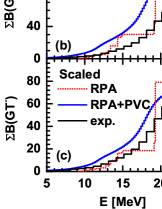
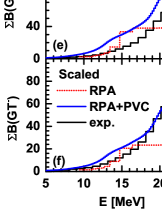
Figure 3: (Color online) Gamow-Teller strength distributions [panels (a), (d), and (g)], their cumulative sums [panels (b), (e), and (h)] and scaled cumulative sums [panels (c), (f), and (i)], calculated with the Skyrme interactions SAMi (first column) and SGII (second and third columns) for the nucleus ²⁰⁸Pb. The red-dotted lines and blue-dashed lines denote the results of RPA and RPA+PVC model, respectively. The smearing parameter $\Delta$ in the calculations is assumed either of the order of the experimental energy resolution ($\Delta=1.0$ MeV, first and second columns), or smaller ($\Delta=0.2$ MeV, third column). The experimental data Wakasa et al. (2012) are displayed by black dots and black solid lines.

In Fig. 3, we show the GT strength distributions, their cumulative sums and the scaled cumulative sums calculated with the Skyrme interactions SAMi and SGII for the nucleus ²⁰⁸Pb, compared with the experimental data of Ref. Wakasa et al. (2012). The excitation energies are given with respect to the parent nucleus in all the figures. The discrete RPA strength is folded with Lorentzian functions having width equal to $2\Delta$. In order to obtain a consistent comparison with data, in panels (a)-(f) we adopt a value $\Delta=1$ MeV, similar to the experimental energy resolution, in both the RPA and RPA+PVC calculations. In panels (g)-(i) we also show the results obtained with a smaller value, namely $\Delta=200$ keV, in order to see the features of the theoretical GT distribution in more detail. The scaled cumulative sums are obtained by scaling both the RPA and RPA+PVC total strength at $E=25$ MeV to the experimental value.

As already seen in Fig. 2, the Skyrme interaction SAMi reproduces the experimental energy of the GTR very well at the RPA level. Including the coupling with phonons, the GT energy is shifted downward, worsening the agreement with the experimental peak energy. On the other hand, the SGII interaction produces a higher GT peak energy compared to the experiment at the RPA level, while the RPA+PVC calculation reproduces very well the line shape of the resonance. Our results are similar to those obtained in the recent relativistic time blocking (RTBA) calculations for ²⁰⁸Pb reported in Ref. Litvinova et al. (2014). Besides the main GT peak at 19.2 MeV, there is another low-energy peak produced by the RPA+PVC calculations, located at about 11.5 MeV (SAMi) or 12.5 MeV (SGII).

Concerning strengths, the total GT^- [$\sum B$(GT^-)] and GT⁺ [$\sum B$(GT⁺)] strengths calculated in the RPA approach with the SGII interaction are 132.95 and 0.96, respectively. The RPA result for $\sum B({\rm GT}^{-})-\sum B({\rm GT}^{+})$ exhausts 99.99% of the Ikeda sum rule. Only 3% of the calculated GT^- strength lies at energies above 25 MeV. In the RPA+PVC calculation, $\sum B({\rm GT}^{-})-\sum B({\rm GT}^{+})$ exhausts 95.2% of the Ikeda sum rule up to the excitation energy 60 MeV while this value becomes 97.3% in the case of smearing parameter $\Delta=0.2$ MeV. About 15% of the sum rule is shifted above $E=25$ MeV [$\sum_{E\leq 25{\rm MeV}}B({\rm GT}^{-})=112.48$, $\sum_{E\leq 25{\rm MeV}}B({\rm GT}^{+})=0.72$]. The experimental strength integrated up to 25 MeV is equal to about 79, corresponding to $71\%$ of the RPA+PVC result Wakasa et al. (2012). This is in agreement with the recent RTBA calculation of Ref. Litvinova et al. (2014), where the ratio between the experimental strength integrated up to 25 MeV and the RTBA result is about 72% using the same smearing parameter $\Delta=1.0$ MeV as ours. Previous studies found that RPA tensor correlations could shift about 10% of the sum rule to the excitation energy region above 30 MeV Bai et al. (2009a, b). The inclusion of $\Delta$-isobar excitation could move strength to very high excitation energy, this amount being of the order of 10% of the total sum rule or less Brown and Wildenthal (1987); Wakasa et al. (1997); Yako et al. (2005). Concerning the remaining discrepancy with experiment, we cannot determine to which extent it can be attributed to deficiencies in the model, or to systematic uncertainties that the experiment was unable to pin down. Despite the disagreement in the total strength, the energy dependence of the cumulative sum calculated with RPA+PVC reproduces quite well the experimental data. In order to see this more clearly, in panel (f) we scale the theoretical integrated strength up to $E=25$ MeV to the experimental value. It can be seen that the inclusion of the phonon coupling improves the description of data considerably as compared to the RPA result. There is some excess in the theoretical strength of the RPA+PVC calculation as compared to the data in the energy region $E=12-16$ MeV, due to the already mentioned low-lying peaks.

By reducing the value of the smearing parameter from $\Delta=1$ MeV to $\Delta=200$ keV [panel (g)], one can investigate the detailed structure of the resonance. The main peak, which had a FWHM equal to 3.6 MeV (cf. Fig. 2 and Table 1), is roughly split into two peaks, located at $E=$ 19.2 MeV and $E=20.6$ MeV, with a FWHM equal to 1.2 and 2 MeV respectively (cf. Table 1). In Ref. Litvinova et al. (2014), the resonance calculated in RTBA is also split into two subpeaks in a very similar way.

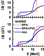
Figure 4: (Color online) The same as Fig. 3, in the case of the nucleus ⁴⁸Ca and the interaction SGII. The experimental data are taken from Ref. Yako et al. (2009).

In keeping with the fact that the effects of PVC depend little on the interaction, in the following we will only display the results calculated with the interaction SGII. In Fig. 4, we show GT results for ⁴⁸Ca. In this case, the experimental energy resolution is about 200 keV, and the experimental strength function Yako et al. (2009) displays a rather complex structure. One finds a low-lying peak at about 3 MeV, with a narrow FHWM of about 0.4 MeV, followed by a broad resonance region between 5 and 16 MeV displaying two peaks lying at 8.2 MeV (with a FWHM of 1.5 MeV) and at 10.8 MeV (with a FWHM of 3.9 MeV); the centroid energy of these two peaks is equal to 10.5 MeV. Finally, a small and narrow peak is observed at 17.5 MeV. The RPA+PVC calculation with the small averaging parameter $\Delta=0.2$ MeV reproduces the strength distribution in the low-energy region reasonably well: the lowest peak energy (2.8 MeV), as well as its FWHM (0.4 MeV), match the experimental values. One finds, then, a very large peak with centroid energy at 10.5 MeV and a much smaller peak at 13.2 MeV. The associated FWHMs are too narrow, being equal to 1.2 MeV and 0.7 MeV respectively (cf. Table 1). The calculation with $\Delta$ = 1 MeV, in which these two peaks merge in a single peak with centroid energy 10.4 MeV and FWHM 2.6 MeV, provides a better overall description of the experimental line shape [cf. panel (d)], as well as a better reproduction of the observed cumulated strength once it is suitably scaled [cf. panel (f)]. The peak appearing at 17.5 MeV in the experiment is not reproduced by the calculation. With $\Delta=0.2$ MeV, the experimental strength integrated up to 20 MeV reaches 63% of the RPA+PVC result. In turn, 8% of the sum rule in the RPA+PVC calculation (2% in the RPA case) is found beyond this interval.

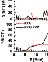
Figure 5: (Color online) Gamow-Teller strength distributions [panels (a) and (c)] with their cumulative sums [panels (b) and (d)] calculated with the Skyrme interaction SGII for the nucleus ¹³²Sn. The red dotted lines and black solid lines denote the results of the RPA and RPA+PVC models, respectively. The smearing parameter $\Delta$ in the calculations takes either a small value $\Delta=0.2$ MeV (first column) or a large one $\Delta=1.0$ MeV (second column).

In the following, we will provide predictions for a few nuclei for which no measurement has been published up to date.

In Fig. 5 we show the GT strength distributions and their cumulative sums for the nucleus ¹³²Sn. Very recently, a (p,n) experiment on ¹³²Sn was carried out at RIKEN with the purpose of studying its GT and spin dipole strength distributions Sasano et al. (2014). In our calculation, using the small averaging parameter $\Delta=0.2$ MeV, the PVC lowers the main RPA peak located at 16 MeV by about 2 MeV and fragments it into three close sub-peaks, which, by using $\Delta=1$ MeV, merge into one broad peak with a FWHM of about 3.6 MeV in the resonance region (cf. Table 1). A secondary RPA peak at about 8 MeV is also shifted downward by 2 MeV. About 1.5% (RPA) and 9% (RPA+PVC with $\Delta$ =0.2 MeV) of the cumulative sum rule is found beyond 20 MeV. The latter value increases up to 15% using $\Delta$ =1 MeV.

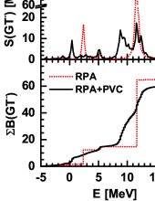
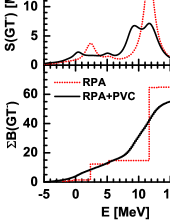
Figure 6: (Color online) The same as Fig. 5 in the case of the nucleus ⁷⁸Ni.

Finally, in Fig. 6 the strength distribution calculated for the nucleus ⁷⁸Ni is shown. This nucleus lies on the r-process path and its $\beta$-decay half-life has a considerable influence on the nuclear abundances around $N=50$ Hosmer et al. (2005). Its $\beta$-decay half-life has been measured Hosmer et al. (2005), and it is quite short ($\approx$ 110 ms) as expected from the large neutron excess so that the measurement of the GT strength distribution definitely represents a very severe challenge. In our calculation, the inclusion of the particle-vibration coupling (calculated with $\Delta=0.2$ MeV) produces in this case a large spreading width and a strong fragmentation of the main RPA resonance peak located at about 11.5 MeV, leading to a two-peak structure (cf. Table 1) centered at 10.7 MeV with a FWHM of about 4.2 MeV. Also the low-lying RPA peak is shifted downward by about 2 MeV and becomes broader. These effects on the low-lying peak could help to reduce the calculated $\beta$-decay half-life which is usually overestimated in the RPA approach Engel et al. (1999); Nikšić et al. (2005); Niu et al. (2013). As for the cumulative sum, 1.3% of the RPA sum rule and 7% of the RPA+PVC sum rule using $\Delta$ =0.2 MeV (11% using $\Delta$ =1 MeV) are found beyond $E=20$ MeV.

III.2 Overall features of Gamow-Teller resonance and phonons

Table 1: Summary of the GTR peak energies and their associated FWHMs extracted from the strength functions of the nuclei we have considered, calculated by the RPA+PVC approach with the interaction SGII. Also shown are available experimental data.

		208Pb	48Ca	132Sn	78Ni
Expt.	$E_{1}$	19.2	8.3
	FWHM1	5.0	1.5
	$E_{2}$		10.9
	FWHM2		3.9
$\Delta=1$ MeV	$E_{1}$	19.6	10.4	14.8	10.5
	FWHM1	3.6	2.6	3.6	5.6
$\Delta=0.2$ MeV	$E_{1}$	19.2	10.4	13.8	8.8
	FWHM1	1.2	0.5	0.7	1.8
	$E_{2}$	20.6	11.2	15	11.6
	FWHM2	2.0	0.7	0.9	1.4
	$E_{3}$		13.2	15.8
	FWHM3		0.7	1.0

In the previous subsection, we have seen that the coupling to vibrations modifies the strength distribution in rather different ways, depending on the specific nucleus. To summarize this feature, the energies of the GTR peaks and the associated FWHMs taken from the strength functions calculated by the RPA+PVC approach with the interaction SGII, are provided in Table 1. Also the available experimental data are shown. Using the value $\Delta=0.2$ MeV, one finds two or three peaks with an overall FWHM of 2 MeV in ⁴⁸Ca, and 3 MeV in ²⁰⁸Pb and in ¹³²Sn, and a broad and strongly fragmented structure in ⁷⁸Ni.

Table 2: The imaginary part of the self-energy multiplied by $-2$ calculated at the RPA energy of the GTR peak in the case of the nuclei ²⁰⁸Pb, ⁴⁸Ca, ¹³²Sn and ⁷⁸Ni with the interaction SGII, using the smearing parameter $\Delta=0.2$ MeV. The partial contributions from phonons with different multipolarities, as well as the total values, are listed.

Nucleus	$-2{\rm Im}\Sigma(1^{-})$	$-2{\rm Im}\Sigma(2^{+})$	$-2{\rm Im}\Sigma(3^{-})$	$-2{\rm Im}\Sigma(4^{+})$	$-2{\rm Im}\Sigma(5^{-})$	$-2{\rm Im}\Sigma$ (total)
208Pb	0.54	0.075	0.89	0.078	0.29	1.88
48Ca	1.0 $\times 10^{-3}$	1.75	0.016	0.20	6.6 $\times 10^{-4}$	1.96
132Sn	0.67	0.30	0.046	0.40	0.030	1.46
78Ni	0.37	0.17	0.22	0.56	$3.1\times 10^{-3}$	1.32

In Table 2, we provide approximate values for the widths of the various nuclei, calculated according to the perturbative expression $\Gamma_{\rm GTR}(E_{\rm RPA})$ [cf. Eq. (17)] with $\Delta$= 0.2 MeV. The partial contributions from phonons with different multipolarities are also listed. These values are approximated ones, as discussed below in the cases of ⁴⁸Ca and ²⁰⁸Pb. However, they provide useful information about the differences and similarities in widths among these nuclei. The $2^{+}$ phonon gives the dominant contribution to the width in ⁴⁸Ca, while only negative-parity phonons are important for ²⁰⁸Pb. The $5^{-}$ multipolarity is relevant only in ²⁰⁸Pb. The other phonons give comparable contributions in ⁷⁸Ni and ¹³²Sn (except for $3^{-}$ in ¹³²Sn).

Table 3: The energies and reduced transition probabilities of the lowest phonons of multipolarity $2^{+},3^{-},4^{+}$, and $5^{-}$ calculated in the RPA with interaction SGII are compared with available experimental data, for the nuclei ²⁰⁸Pb, ⁴⁸Ca, ¹³²Sn, and ⁷⁸Ni. The experimental data are taken from Refs. http://www.nndc.bnl.gov ; Martin (2007); Khazov et al. (2005); Burrows (2006). The calculated phonon states shown in parentheses have a strength smaller than 5% of the total isoscalar or isovector strength, and therefore are not included in the PVC calculation.

			208Pb	48Ca	132Sn	78Ni
$2^{+}$	Expt.	$E$ (MeV)	4.09	3.83	4.04
		$B(EL,0\rightarrow L)$(e2 fm4)	$3.10\times 10^{3}$	88.84	$1.39\times 10^{3}$
		$B(EL)$ (s.p.u.)	8.5	1.7	7.0
	Theor.	$E$ (MeV)	5.03	3.80	4.54	3.46
		$B(EL,0\rightarrow L)$(e2 fm4)	$2.74\times 10^{3}$	51.82	$1.10\times 10^{3}$	$3.83\times 10^{2}$
		$B(EL)$ (s.p.u.)	7.5	1.0	5.5	3.9
$3^{-}$	Expt.	$E$ (MeV)	2.62	4.51	4.35
		$B(EL,0\rightarrow L)$(e2 fm6)	$6.12\times 10^{5}$	$4.82\times 10^{3}$	$>5.14\times 10^{4}$
		$B(EL)$ (s.p.u.)	34.1	5.0	$>7.1$
	Theor.	$E$ (MeV)	3.09	5.75	5.29	7.61
		$B(EL,0\rightarrow L)$(e2 fm6)	$6.79\times 10^{5}$	$8.02\times 10^{3}$	$1.19\times 10^{5}$	$1.68\times 10^{4}$
		$B(EL)$ (s.p.u.)	37.7	8.4	16.5	6.6
$4^{+}$	Expt.	$E$ (MeV)	4.32	4.50	4.42
		$B(EL,0\rightarrow L)$(e2 fm8)	$1.62\times 10^{7}$		$2.17\times 10^{6}$
		$B(EL)$ (s.p.u.)	18.8		8.0
	Theor.	$E$ (MeV)	4.96	(4.13)	5.00	4.22
		$B(EL,0\rightarrow L)$(e2 fm8)	$9.77\times 10^{6}$	($6.82\times 10^{3}$)	$2.08\times 10^{6}$	$2.12\times 10^{5}$
		$B(EL)$ (s.p.u.)	11.4	(0.4)	8.1	3.4
$5^{-}$	Expt.	$E$ (MeV)	3.20	5.73	4.94
		$B(EL,0\rightarrow L)$(e2 fm10)	$4.47\times 10^{8}$
		$B(EL)$ (s.p.u.)	11.0
	Theor.	$E$ (MeV)	3.76	(7.28)	6.85	(8.11)
		$B(EL,0\rightarrow L)$(e2 fm10)	$4.64\times 10^{8}$	($1.58\times 10^{6}$)	$2.43\times 10^{7}$	($2.61\times 10^{3}$)
		$B(EL)$ (s.p.u.)	11.4	(5.1)	2.7	(0.0017)

These different behaviors are mostly determined by the properties of the lowest phonons and by the underlying shell structure in each nucleus. In Table 3 we report the energies and reduced transition probabilities of the lowest phonons with multipolarity $2^{+},3^{-},4^{+}$, and $5^{-}$ calculated within RPA for all these nuclei, comparing them with available experimental data. In most cases, the states have rather collective character, their reduced transition probabilities being of the order of several single-particle units (s.p.u.). For ²⁰⁸Pb and ¹³²Sn, both the energies and reduced transition probabilities agree well with the experimental data. In the case of ⁴⁸Ca, although the calculated phonon energies agree well with the data, the theoretical and experimental reduced transition probabilities differ by about 40%: theory underestimates the B(E2) value and overestimates the B(E3) value. Since among the 2⁺ phonons that provide a dominant contribution to the width, the lowest 2⁺ state plays a major role, we can argue that the calculated width would be approximately doubled if the B(E2) value were enlarged by the same factor, in which case the experimental width would be well reproduced. Thus, the calculated width might be underestimated not due to a basic failure in our picture but rather to the fact that RPA does not account well in this case for the collectivity of the low-lying 2⁺ phonon.

III.3 Underlying mechanisms for the spreading width and fragmentation

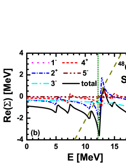
Figure 7: (Color online) The imaginary part multiplied by $-2$ [panel (a)] and the real part [panel(b)] of the self-energy of the main RPA state for the nucleus ⁴⁸Ca, calculated by the interaction SGII with a smearing parameter $\Delta=0.2$ MeV. In addition to the total results, the contributions from phonons with different multipolarities are shown separately. The vertical short-dotted-olive line represents the energy position $E_{\rm RPA}$ of the GTR peak calculated in the RPA approach, while the dashed line in panel (b) represents the function $y=E-E_{\rm RPA}$.

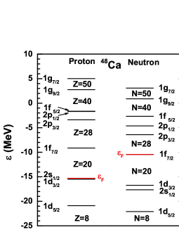
Figure 8: (Color online) Proton and neutron single-particle spectrum in ⁴⁸Ca obtained from the HF calculation with SGII interaction.

In this subsection we will discuss in more detail the microscopic processes leading to the damping of the GT resonance. We start by considering the case of ⁴⁸Ca, calculated with $\Delta$ = 0.2 MeV. Looking at Tables 1 and 2 and Fig. 7, we observe that

(i) The calculated strength function displays three peaks located at 10.4, 11.2 and 13.2 MeV, with associated widths equal to 0.5, 0.7, and 0.7 MeV.

(ii) The dominant contribution to the width is provided by the coupling to quadrupole phonons; $4^{+}$ phonons become important beyond 13 MeV (cf. Fig. 7). The contributions from negative parity phonons are negligible.

The result (i) obtained in the full diagonalization can be quantitatively reproduced by the much simpler expressions with diagonal approximation Eqs. (16) and (17), in which the self-energy $\Sigma_{\rm GTR}(\omega)$ for the giant resonance state is given by the energy-dependent matrix element $({\cal A}_{1})_{\rm GTR,GTR}(E)$. For convenience we reproduce the equations here, in a slightly different form:

$$E_{\rm GTR}-E_{\rm RPA}={\rm Re}[({\cal A}_{1})_{\rm GTR,GTR}(E_{\rm GTR})]$$ (18)

and

$$\Gamma_{\rm GTR}(E_{\rm GTR})=-2{\rm Im}[({\cal A}_{1})_{\rm GTR,GTR}(E_{\rm GTR})].$$ (19)

The curve ${\rm Re}[({\cal A}_{1})_{\rm GTR,GTR}(E)]$ and the line $y=E-E_{\rm RPA}$ are plotted in panel (b) of Fig. 7. They cross at $E$= 10.4 MeV. Furthermore, the quantity $|y-{\rm Re}[\Sigma_{\rm GTR}(E)]|$ has two minima very close to 0 at $E=11.2$ and $13.2$ MeV. These values give the GTR peak energies $E_{\rm GTR}$. Correspondingly, the widths $\Gamma_{\rm GTR}(E_{\rm GTR})$ for $E_{GTR}$ = 10.4,11.2, and 13.2 are given by 0.40, 0.79, and 2.52 MeV , respectively. These values of the energies and widths are in very good agreement with the complex eigenvalues resulting from the full solution which are $10.30-i0.41$ MeV, $10.76-i0.83$ MeV, and $12.96-i2.36$ MeV, where the imaginary parts have been multiplied by 2 to obtain the width. The first two values correspond well to the FWHMs (0.5 and 0.7 MeV) extracted from the strength distribution (cf. Table 1). However, the FWHM of the third peak at $13.2$ MeV obtained from the strength function is 0.7 MeV, smaller than the value given above due to the sharp decrease of the imaginary part of the self-energy above the peak energy [cf. panel (a) of Fig. 7].

In order to understand the feature (ii), we need to determine the configurations which give the largest contributions to the particle and hole self-energies, i.e., diagrams (1) and (2) of Fig. 1. The microscopic RPA wave function of the GTR in ⁴⁸Ca is dominated by a single p-h transition of energy 8.84 MeV, namely $\nu 1{\rm f}_{7/2}\rightarrow\pi 1{\rm f}_{5/2}$. In diagram (1) (cf. Fig. 1), the most important intermediate proton particle states $p^{\prime\prime}$ and phonons $nL$ are those being able to couple with the $\pi 1{\rm f}_{5/2}$ proton state and minimize the denominator $\Omega_{\rm GTR}-(\omega_{nL}+\epsilon_{\pi p^{\prime\prime}}-\epsilon_{\nu 1{\rm f}_{7/2}})+i\Delta$ in Eq. (II). The GTR energy is given approximately by the energy of the particle-hole transition, plus a shift $\Delta E$, which takes into account the effects of the repulsive p-h interaction and of the PVC (cf. Fig. 2). When we use a small value of the smearing parameter $\Delta$, several peaks may appear in the strength distribution (cf. Fig. 4). For simplicity, in the following approximate analysis, we shall use the RPA energy $E_{\rm RPA}$ instead of $\Omega_{\rm GTR}$, and neglect the PVC effect on $\Delta E$. We then put $E_{\rm RPA}=\epsilon_{\pi 1{\rm f}_{5/2}}-\epsilon_{\nu 1{\rm f}_{7/2}}+\Delta E$, so that the denominator becomes $\epsilon_{\pi 1{\rm f}_{5/2}}-\epsilon_{\pi p^{\prime\prime}}-\omega_{nL}+\Delta E+i\Delta$. This means that the relevant intermediate states must lie at an energy $\epsilon_{\pi p^{\prime\prime}}\approx\epsilon_{\pi 1{\rm f}_{5/2}}-\omega_{nL}+\Delta E$. Given that typical values for the energies of the low-lying collective phonons $\omega_{nL}$ are 3-4 MeV and $\Delta E=3$ MeV, this requires that $p^{\prime\prime}$ lies close to $\pi 1{\rm f}_{5/2}$. Looking at Fig. 8, one realizes that this condition is fulfilled only by negative parity single-particle levels in the $pf$ shell, which can couple to the state $\pi 1{\rm f}_{5/2}$ only through positive parity phonons. In a similar way, for diagram (2) (cf. Fig. 1) the energy of the intermediate neutron hole states $\nu h^{\prime\prime}$ coupling to the $\nu 1{\rm f}_{7/2}$ neutron state and giving important contribution to the GTR width is restricted by the condition $\epsilon_{\nu h^{\prime\prime}}\approx\epsilon_{\nu 1{\rm f}_{7/2}}+\omega_{nL}-\Delta E$. Since the $\nu 1{\rm f}_{7/2}$ state is isolated (cf. Fig. 8), this relation can only be satisfied by coupling the $\nu 1{\rm f}_{7/2}$ state with itself through positive parity phonons. In conclusion, the positive parity low-lying phonons rather than the negative parity ones give important contributions to the width because the particle and hole states of the dominant transition are isolated with other single-particle states or close to the states with the same parity, since the energy of low-lying phonons is usually similar to the energy shift $\Delta E$.

More generally, we can conclude from the previous discussion that when the GTR wavefunction is dominated by a strong $\nu l_{j_{>}}\rightarrow\pi l_{j_{<}}$ transition, the intermediate proton particle states $\pi p^{\prime\prime}$ or neutron hole states $\nu h^{\prime\prime}$ and the phonons will obey the following relation if the corresponding diagram gives important contributions to the GTR spreading width,

$$\epsilon_{\pi p^{\prime\prime}}\approx\epsilon_{\pi lj_{<}}-\omega_{nL}+\Delta E\quad{\rm and}\quad\epsilon_{\nu h^{\prime\prime}}\approx\epsilon_{\nu lj_{>}}+\omega_{nL}-\Delta E,$$ (20)

where $\Delta E$ is the energy difference between the energy of p-h configuration and the energy of the GTR peak (approximated by the energy of RPA peak).

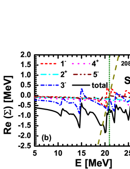
Figure 9: (Color online) The same as Fig. 7 in the case of the nucleus ²⁰⁸Pb.

We now turn to the case of ²⁰⁸Pb. In Fig. 9, we display the values of the imaginary part and real part of the self-energy for the GTR state from RPA calculation, in the same fashion as we did for ⁴⁸Ca. The zeros or the minima of the function $|E-E_{\rm GTR}-{\rm Re}[\Sigma_{\rm GTR}(E)]|$, in the present case lie at $E=19.4$ and 20.4 MeV [cf. panel(b) of Fig. 9], that correspond well to the peak energies (19.2 and 20.6 MeV) reported in Table 1. From panel (a) of Fig. 9, we obtain that the widths at these two peak energies are 1.0 and 2.2 MeV, which again are in agreement with the FWHMs (1.2 and 2 MeV) reported in Table 1.

The individual contributions to the self-energy from the various phonon multipolarities are also shown in Fig. 9, and the corresponding values of the imaginary part of the self-energy calculated at the RPA energy $E_{\rm RPA}$ are given in Table 2. Phonons of positive parity give negligible contributions in this nucleus. This is mainly due to the cancellation between self-energy diagrams [(1) and (2)] and the phonon exchange diagrams [(3) and (4)] of Fig. 1. This cancellation, which does not play so important role in ⁴⁸Ca, becomes more severe for large single-particle angular momentum, which occurs in the case of ²⁰⁸Pb Bortignon (1981). We also observe that the contribution from the $1^{-}$ phonons to the GTR width (0.44 MeV) is comparable to that from $3^{-}$ (1.05 MeV) and $5^{-}$ phonons (0.30 MeV). The $1^{-}$ contribution is also important in ⁷⁸Ni and in ¹³²Sn. This may appear surprising, if one sticks to the general prejudice that the largest effects usually originate from low-energy phonons.

Table 4: Contributions to self-energy $({\cal A}_{1})^{\rm GTR,GTR}_{php^{\prime}h^{\prime}}(E_{\rm RPA})$ arising from the two most important particle-hole configurations forming the GTR state in ²⁰⁸Pb, and associated with the coupling to $1^{-}$ phonons. The calculation is performed with the interaction SGII and smearing parameter $\Delta=0.2$ MeV. The self-energy is calculated at the RPA energy of the GTR. $i^{\prime\prime}$ labels the intermediate particle or hole state of the diagrams, and $E_{1^{-}}$ is the energy of the $1^{-}$ phonon state. For given $ph$ and $p^{\prime}h^{\prime}$ configurations, first we provide the total value of $W^{\downarrow}_{ph,p^{\prime}h^{\prime}}$ as well as the value of $({\cal A}_{1})^{\rm GTR,GTR}_{php^{\prime}h^{\prime}}(E_{\rm RPA})$. In the following four lines, the individual values $W_{kph,p^{\prime}h^{\prime}}$ ($k=1,...,4$) are given. In the fifth line we give the contribution to $W^{\downarrow}$ and $({\cal A}_{1})^{\rm GTR,GTR}$ arising from the most important diagram contributing to the width, associated with a single intermediate state $i^{\prime\prime}=p^{\prime\prime}$ or $i^{\prime\prime}=h^{\prime\prime}$. In the last line labeled with “Total”, the value of $({\cal A}_{1})^{\rm GTR,GTR}_{php^{\prime}h^{\prime}}(E_{\rm RPA})$ summed over all $ph,p^{\prime}h^{\prime}$ particle-hole configurations of the RPA model space is given. The notation (a,b) represents the complex number $a+ib$.

$ph$	$p^{\prime}h^{\prime}$	$X^{\rm GTR}_{ph}$	$X^{\rm GTR}_{p^{\prime}h^{\prime}}$	$i^{\prime\prime}$	$E_{1^{-}}$ (MeV)	$W^{\downarrow}_{php^{\prime}h^{\prime}}$ (MeV)	$({\cal A}_{1})^{\rm GTR,GTR}_{php^{\prime}h^{\prime}}$ (MeV)
$\pi 1{\rm h}_{9/2}-\nu 1{\rm h}_{11/2}$	$\pi 1{\rm h}_{9/2}-\nu 1{\rm h}_{11/2}$	-0.51	-0.51			(-0.094, -0.31)	(-0.025, -0.083)
						$W_{1}$ (-0.019, -1.88$\times 10^{-4}$)
						$W_{2}$ (-0.076, -0.31)
						$W_{3}$ (0,0)
						$W_{4}$ (0,0)
				h” $\nu 1{\rm i}_{13/2}$	12.63	$W_{2}$ (-0.30,-0.095)	( 0.080,-0.025)
				h” $\nu 1{\rm i}_{13/2}$	13.62	$W_{2}$ (-0.37,-0.21)	(-0.099, -0.056)
$\pi 1{\rm h}_{9/2}-\nu 1{\rm h}_{11/2}$	$\pi 1{\rm i}_{11/2}-\nu 1{\rm i}_{13/2}$	-0.51	-0.76			(0.10,-0.17)	(0.040,-0.065) $\times 2$
						$W_{1}$ (0,0)
						$W_{2}$ (0,0)
						$W_{3}$ (0.11, -0.17)
						$W_{4}$ (-8.00$\times 10^{-3}$, -9.23$\times 10^{-5}$ )
					12.63	$W_{3}$ (0.25,-0.078)	(0.066,-0.021)
					13.62	$W_{3}$ (-0.15,-0.084)	(-0.039,-0.022)
$\pi 1{\rm i}_{11/2}-\nu 1{\rm i}_{13/2}$	$\pi 1{\rm i}_{11/2}-\nu 1{\rm i}_{13/2}$	-0.76	-0.76			(0.089, -0.10)	(0.051, -0.060)
						$W_{1}$ (0.10, -0.10)
						$W_{2}$ (-0.012, -1.38$\times 10^{-4}$)
						$W_{3}$ (0,0)
						$W_{4}$ (0,0)
				p” $\pi 1{\rm h}_{9/2}$	12.63	$W_{1}$ (0.21,-0.064)	(0.12, -0.037)
Total							(0.10,-0.27)

Figure 10: (Color online) Proton and neutron single-particle spectrum in ²⁰⁸Pb obtained from the HF calculation with the SGII interaction.

We study the reasons for the relevance of the $1^{-}$ phonons in Table 4. There are two important p-h configurations entering the RPA wave function of the GTR in ²⁰⁸Pb with forwards-going RPA amplitudes in absolute value larger than 0.5, namely $\pi 1{\rm h}_{9/2}-\nu 1{\rm h}_{11/2}$ and $\pi 1{\rm i}_{11/2}-\nu 1{\rm i}_{13/2}$. In Table 4 we list the contributions to the self-energy $({\cal A}_{1})^{\rm GTR,GTR}_{ph,p^{\prime}h^{\prime}}(E_{\rm RPA})$ associated with a $ph$, $p^{\prime}h^{\prime}$ pair, and arising from the coupling of these $ph$ configurations with the $1^{-}$ phonons. The leading role is played by two collective $1^{-}$ phonons which carry the strongest isovector transition strength and have energies $E_{1^{-}}$= 12.63 and 13.62 MeV [i.e., isovector giant dipole resonance (IVGDR) components]. Note that due to parity conservation $W_{3}$ and $W_{4}$ vanish when $ph=p^{\prime}h^{\prime}$, and $W_{1},W_{2}$ vanish when $ph\neq p^{\prime}h^{\prime}$. For the diagonal matrix element $W_{ph,ph}$ in the case of $\pi 1{\rm h}_{9/2}-\nu 1{\rm h}_{11/2}$, the most important contribution to the width comes from the diagram $W_{2}$, associated with the self-energy of the hole $\nu 1{\rm h}_{11/2}$. We can then use Eq. (20) with $\omega_{nL}\approx$ 13 MeV and $\Delta E=E_{\rm RPA}-(\epsilon_{\pi 1{\rm h}_{9/2}}-\epsilon_{\nu 1{\rm h}_{11/2}})=6$ MeV, and find that the important intermediate neutron hole states coupling to the $1^{-}$ phonon and to the $\nu 1h_{11/2}$ hole must lie at an energy $\epsilon_{\nu h^{\prime\prime}}\approx\epsilon_{\nu 1h_{11/2}}+13-6=-11$ MeV, which is close to the energy of the ${\nu 1i_{13/2}}$ hole state ($\epsilon_{\nu{i}_{13/2}}$ = -10.5 MeV). So the intermediate hole state $\nu 1i_{13/2}$ could be coupled to $\nu 1h_{11/2}$ state and gives a non-negligible $W_{2}$ value. In a similar way, for the diagonal matrix element $W_{ph,ph}$ in the case of $\pi 1i_{11/2}-\nu 1i_{13/2}$, with $\Delta E=E_{\rm RPA}-(\epsilon_{\pi 1i_{11/2}}-\epsilon_{\nu 1i_{13/2}})=3.5$ MeV, we find that important proton particle states coupling to the $1^{-}$ phonon and to the $\pi 1i_{11/2}$ state should satisfy the condition $\epsilon_{\pi p^{\prime\prime}}\approx\epsilon_{\pi 1i_{11/2}}-13+3.5=-2.5$ MeV, which is well fulfilled by the $\pi 1h_{9/2}$ orbital, lying at -3 MeV. Besides these contributions associated with the diagrams $W_{1}$ and $W_{2}$, in the present case one finds an important contribution also from diagram $W_{3}$ associated with the non-diagonal matrix element of the configuration $\pi 1{\rm i}_{11/2}-\nu 1{\rm i}_{13/2}$ and $\pi 1{\rm h}_{9/2}-\nu 1{\rm h}_{11/2}$. The non-diagonal matrix element contributes twice since the two different configurations could be exchanged with each other. In conclusion, the IVGDR phonons can give important contributions to the GTR width when an intermediate particle (hole) state lies below (above) the particle (hole) state associated with an important GT configuration by $1\hbar\omega$ energy difference, which can be compensated by the energy of collective dipole phonon. This condition can be satisfied in nuclei characterized by large isospin in which the GT state is composed of two or more important p-h configurations.

The reason for the importance of ${1^{-}}$ phonons in ⁷⁸Ni and ¹³²Sn appears to be analogous to the case of ²⁰⁸Pb. In these two nuclei the RPA wave function of the GTR is dominated by two p-h configurations: $\pi 1{\rm g}_{7/2}-\nu 1{\rm g}_{9/2}$ and $\pi 1{\rm h}_{9/2}-\nu 1{\rm h}_{11/2}$ in ¹³²Sn, or $\pi 1{\rm f}_{5/2}-\nu 1{\rm f}_{7/2}$ and $\pi 1{\rm g}_{7/2}-\nu 1{\rm g}_{9/2}$ in ⁷⁸Ni. In the case of ¹³²Sn (⁷⁸Ni) the energy difference between the GTR and the collective giant dipole state $E_{\rm GTR}-\omega_{nL}$ is about 1.0 MeV (-5.3 MeV), which is close to the energy 0.5 MeV (-6.1 MeV) of the p-h configuration $\pi 1{\rm g}_{7/2}-\nu 1{\rm h}_{11/2}$ ($\pi 1{\rm f}_{5/2}-\nu 1{\rm g}_{9/2}$), i.e., $\epsilon_{p^{\prime\prime}}-\epsilon_{h}$ or $\epsilon_{p}-\epsilon_{h^{\prime\prime}}$. These two nuclei are similar, also in the sense that the multipolarities $1^{-}$, $2^{+}$ and $4^{+}$ give comparable contributions, and so do the $3^{-}$ phonons for ⁷⁸Ni. In ⁷⁸Ni, the $3^{-}$ phonons cannot produce spreading width through their coupling to the most important configurations $\pi 1{\rm g}_{7/2}-\nu 1{\rm g}_{9/2}$ or $\pi 1{\rm f}_{5/2}-\nu 1{\rm f}_{7/2}$, due to the fact that the hole states of these configurations are isolated from the other levels while the particle states are close to the states with the same parity, as in the case of ⁴⁸Ca. However, the $3^{-}$ phonons produce some width by coupling to the p-h configuration $\pi 2{\rm p}_{3/2}-\nu 2{\rm p}_{3/2}$.

IV Conclusion

Many studies of the GTR are performed at the mean-field level. However, experiment shows that such a resonance has a conspicuous width, coming mainly from coupling to complex nuclear configurations. Benchmarking nuclear models through their capability to reproduce at the same time not only energies and strengths, but also widths of the GT states, is not very much pursued - the only exception being probably the recent work of Ref. Litvinova et al. (2014). In the present work, we wish to test systematically a microscopic model, in which on top of HF+RPA the particle-vibration coupling is introduced based consistently on the use of a Skyrme-type force.

In this paper we have applied our model to the cases of ⁴⁸Ca, ⁷⁸Ni, ¹³²Sn, and ²⁰⁸Pb, which can be well described as doubly closed shell nuclei. In the future we plan to include pairing correlations for systematic calculations in open shell nuclei. Our results account well for the experimental findings in ²⁰⁸Pb, especially concerning the lineshape of the GT strength. For ⁴⁸Ca, the experimental width and fragmentation is partly reproduced by the coupling with phonons. We have made predictions for the exotic nuclei ⁷⁸Ni and ¹³²Sn. Large spreading widths and strong fragmentation are obtained for these two nuclei.

For ²⁰⁸Pb the experimental strength integrated up to E = 25 MeV is 71% of the RPA+PVC result, while for ⁴⁸Ca this value up to 20 MeV is 63%. So, we can conclude that the coupling with phonons can produce some quenching of the main GTR, but also other effects, like the inclusion of tensor force and the coupling with high-energy, uncorrelated 2p-2h configurations, need to be considered.

The mechanism for the spreading width and fragmentation is analyzed in detail, particularly in the case of the two nuclei ⁴⁸Ca and ²⁰⁸Pb. To a large extent, the diagonal approximation holds well in the sense that the real part and imaginary part of the self-energy associated with the RPA resonance state calculated at the GTR peak energy account quite well for the energy shift and width of GTR, respectively, produced by the particle-vibration coupling in the full diagonalization. The importance of phonons with different multipolarities is also discussed in detail. The energies of phonons are important for minimizing the energy denominators in the self-energy, whereas the reduced transition probabilities of the phonons influence the matrix elements of the particle-vibration coupling vertex. General arguments may suggest that low-lying phonons are the most effective, in this respect, in particular in order to produce small energy denominators. We have also found, nonetheless, that in nuclei characterized by a large neutron excess, such as ⁷⁸Ni, ¹³²Sn, and ²⁰⁸Pb, the isovector giant dipole phonons can give important contributions to the width. In fact, their energy can match the energy difference between either the particles or holes associated with two important GT configurations.

Comparing the phonon energy and reduced transition probability between the experiment and theory, the phonon properties of ²⁰⁸Pb are best described, while in ⁴⁸Ca the reduced transition probabilities are not reproduced well. This may indicate that the difference in the quality of the results between ²⁰⁸Pb on the one side, and ⁴⁸Ca on the other side, is not due to a breakdown of our overall physical picture, but rather to the inaccurate reproduction of the experimental properties of the low-lying phonons with the adopted interaction.

ACKNOWLEDGMENTS

This work was partly supported by the National Natural Science Foundation of China under Grants No. 11305161.

References

- Osterfeld (1992) F. Osterfeld, Rev. Mod. Phys. 64, 491 (1992).
- Ichimura et al. (2006) M. Ichimura, H. Sakai, and T. Wakasa, Prog. Part. Nucl. Phys. 56, 446 (2006).
- Navarro and Polls (2013) J. Navarro and A. Polls, Phys. Rev. C 87, 044329 (2013).
- Chamel and Goriely (2010) N. Chamel and S. Goriely, Phys. Rev. C 82, 045804 (2010).
- Colò et al. (2014) G. Colò, U. Garg, and H. Sagawa, Eur. Phys. J. A 50, 26 (2014).
- Sagawa et al. (1993) H. Sagawa, I. Hamamoto, and M. Ishihara, Phys. Lett. B 303, 215 (1993).
- Kobayashi et al. (2014) M. Kobayashi, K. Yako, S. Shimoura, M. Dozono, S. Kawase, K. Kisamori, Y. Kubota, C. Lee, S. Michimasa, H. Miya, et al., JPS Conf. Proc. 1, 013034 (2014).
- Langanke and Martínez-Pinedo (2003) K. Langanke and G. Martínez-Pinedo, Rev. Mod. Phys. 75, 819 (2003).
- Janka et al. (2007) H.-T. Janka, K. Langanke, A. Marek, G. Martínez-Pinedo, and B. Müller, Phys. Rep. 442, 38 (2007).
- Paar et al. (2009) N. Paar, G. Colò, E. Khan, and D. Vretenar, Phys. Rev. C 80, 055801 (2009).
- Niu et al. (2011) Y. F. Niu, N. Paar, D. Vretenar, and J. Meng, Phys. Rev. C 83, 045807 (2011).
- Fantina et al. (2012) A. F. Fantina, E. Khan, G. Colò, N. Paar, and D. Vretenar, Phys. Rev. C 86, 035805 (2012).
- Burbidge et al. (1957) E. M. Burbidge, G. R. Burbidge, W. A. Fowler, and F. Hoyle, Rev. Mod. Phys. 29, 547 (1957).
- Qian and Wasserburg (2007) Y.-Z. Qian and G. J. Wasserburg, Phys. Rep. 442, 237 (2007).
- Niu et al. (2013) Z. M. Niu, Y. F. Niu, H. Z. Liang, W. H. Long, T. Nikšić, D. Vretenar, and J. Meng, Phys. Lett. B 723, 172 (2013).
- Avignone et al. (2008) F. T. Avignone, S. R. Elliott, and J. Engel, Rev. Mod. Phys. 80, 481 (2008).
- Vergados et al. (2012) J. D. Vergados, H. Ejiri, and F. Šimkovic, Rep. Prog. Phys. 75, 106301 (2012).
- Auerbach and Klein (1984) N. Auerbach and A. Klein, Phys. Rev. C 30, 1032 (1984).
- Hamamoto and Sagawa (2000) I. Hamamoto and H. Sagawa, Phys. Rev. C 62, 024319 (2000).
- Bender et al. (2002) M. Bender, J. Dobaczewski, J. Engel, and W. Nazarewicz, Phys. Rev. C 65, 054322 (2002).
- Fracasso and Colò (2007) S. Fracasso and G. Colò, Phys. Rev. C 76, 044307 (2007).
- Bai et al. (2009a) C. L. Bai, H. Sagawa, H. Q. Zhang, X. Z. Zhang, G. Colò, and F. R. Xu, Phys. Lett. B 675, 28 (2009a).
- Roca-Maza et al. (2012) X. Roca-Maza, G. Colò, and H. Sagawa, Phys. Rev. C 86, 031306 (2012).
- Martini et al. (2014) M. Martini, S. Péru, and S. Goriely, Phys. Rev. C 89, 044306 (2014).
- De Conti et al. (2000) C. De Conti, A. P. Galeao, and F. Krmpotic, Phys. Lett. B 494, 46 (2000).
- Paar et al. (2004) N. Paar, T. Nikšić, D. Vretenar, and P. Ring, Phys. Rev. C 69, 054303 (2004).
- Liang et al. (2008) H. Z. Liang, N. Van Giai, and J. Meng, Phys. Rev. Lett. 101, 122502 (2008).
- Drożdż et al. (1990) S. Drożdż, S. Nishizaki, J. Speth, and J. Wambach, Phys. Rep. 197, 1 (1990).
- Kuzmin and Soloviev (1984) V. A. Kuzmin and V. G. Soloviev, J. Phys. G 10, 1507 (1984).
- Dang et al. (1997) N. D. Dang, A. Arima, T. Suzuki, and S. Yamaji, Phys. Rev. Lett. 79, 1638 (1997).
- Bertsch et al. (1983) G. F. Bertsch, P. F. Bortignon, and R. A. Broglia, Rev. Mod. Phys. 55, 287 (1983).
- Niu et al. (2012) Y. F. Niu, G. Colò, M. Brenna, P. F. Bortignon, and J. Meng, Phys. Rev. C 85, 034314 (2012).
- Colò et al. (1994) G. Colò, N. Van Giai, P. F. Bortignon, and R. A. Broglia, Phys. Rev. C 50, 1496 (1994).
- Litvinova et al. (2014) E. Litvinova, B. A. Brown, D.-L. Fang, T. Marketin, and R. G. T. Zegers, Phys. Lett. B 730, 307 (2014).
- Harakeh and van der Woude (2001) M. Harakeh and A. van der Woude, Giant resonances: fundamental high-frequency modes of nuclear excitation (Clarendon Press, Oxford, 2001).
- Reinhard and Flocard (1995) P.-G. Reinhard and H. Flocard, Nucl. Phys. A 584, 467 (1995).
- Bartel et al. (1982) J. Bartel, P. Quentin, M. Brack, C. Guet, and H.-B. Håkansson, Nucl. Phys. A 386, 79 (1982).
- Van Giai and Sagawa (1981) N. Van Giai and H. Sagawa, Phys. Lett. B 106, 379 (1981).
- Wakasa et al. (2012) T. Wakasa, M. Okamoto, M. Dozono, K. Hatanaka, M. Ichimura, S. Kuroita, Y. Maeda, H. Miyasako, T. Noro, T. Saito, et al., Phys. Rev. C 85, 064606 (2012).
- Bai et al. (2009b) C. L. Bai, H. Q. Zhang, X. Z. Zhang, F. R. Xu, H. Sagawa, and G. Colò, Phys. Rev. C 79, 041301 (2009b).
- Brown and Wildenthal (1987) B. A. Brown and B. H. Wildenthal, Nucl. Phys. A 474, 290 (1987).
- Wakasa et al. (1997) T. Wakasa, H. Sakai, H. Okamura, H. Otsu, S. Fujita, S. Ishida, N. Sakamoto, T. Uesaka, Y. Satou, M. B. Greenfield, et al., Phys. Rev. C 55, 2909 (1997).
- Yako et al. (2005) K. Yako, H. Sakai, M. Greenfield, K. Hatanaka, M. Hatano, J. Kamiya, H. Kato, Y. Kitamura, Y. Maeda, C. Morris, et al., Phys. Lett. B 615, 193 (2005).
- Yako et al. (2009) K. Yako, M. Sasano, K. Miki, H. Sakai, M. Dozono, D. Frekers, M. B. Greenfield, K. Hatanaka, E. Ihara, M. Kato, et al., Phys. Rev. Lett. 103, 012503 (2009).
- Sasano et al. (2014) M. Sasano, et al., experiment NP1306-SAMURAI17, (2014).
- Hosmer et al. (2005) P. T. Hosmer, H. Schatz, A. Aprahamian, O. Arndt, R. R. C. Clement, A. Estrade, K.-L. Kratz, S. N. Liddick, P. F. Mantica, W. F. Mueller, et al., Phys. Rev. Lett. 94, 112501 (2005).
- Engel et al. (1999) J. Engel, M. Bender, J. Dobaczewski, W. Nazarewicz, and R. Surman, Phys. Rev. C 60, 014302 (1999).
- Nikšić et al. (2005) T. Nikšić, T. Marketin, D. Vretenar, N. Paar, and P. Ring, Phys. Rev. C 71, 014308 (2005).
- (49) http://www.nndc.bnl.gov.
- Martin (2007) M. J. Martin, Nucl. Data Sheets 108, 1583 (2007).
- Khazov et al. (2005) Y. Khazov, A. A. Rodionov, S. Sakharov, and B. Singh, Nucl. Data Sheets 104, 497 (2005).
- Burrows (2006) T. W. Burrows, Nucl. Data Sheets 107, 1747 (2006).
- Bortignon (1981) P. F. Bortignon, R. A. Broglia, Nucl. Phys. A 371, 405 (1981).