Condensation and equilibration in an urn model

Abstract

After reviewing the general scaling properties of aging systems, we present a numerical study of the slow evolution induced in the zeta urn model by a quench from a high temperature to a lower one where a condensed equilibrium phase exists. By considering both one-time and two-time quantities we show that the features of the model fit into the general framework of aging systems. In particular, its behavior can be interpreted in terms of the simultaneous existence of equilibrated and aging degrees with different scaling properties.

1 Introduction

Slow relaxation [1, 2, 3, 4, 5, 6] is the process whereby a system evolves without reaching equilibrium in finite times. Physical realizations of this phenomenon are observed in many materials, for instance ferromagnets, binary or complex fluids and glasses, when they are subjected to a drastic change of thermodynamic control parameters, as in a temperature quench or a pressure crunch. In the large-time regime these systems exhibit typical features of equilibrium, such as the absence of macroscopic currents and the constancy of one-time observables, together with hallmarks of non-stationarity, like the lack of time-reversal invariance and the dependence of two-time quantities on the system’s age $t_{w}$, i.e., the time elapsed after the initial change of parameters.

These apparently contrasting features can be interpreted in a coherent way if the degrees of freedom of the non-equilibrium state can be classified into groups with different properties [7, 8]. In the simplest cases, including ferromagnetic systems and the model considered in this paper, this amounts to identify those degrees whose evolution is sufficiently fast and unrelated to the global non-equilibrium condition of the system to rapidly self-equilibrate with respect to the new value of the control parameters. These fast degrees, whose collection we will indicate with $\{\psi\}$ in the following, are responsible for the appearance of the typical features of equilibrated systems discussed above. The rest of the system – constrained degrees which are not able to efficiently equilibrate with respect to the new control parameters – are a slow component, denoted here with $\{\sigma\}$, which gives rise to the aging properties, namely non-stationarity and lack of time-reversal invariance.

This separation into two classes is fundamental to understand the properties of aging systems: the possibility to disentangle global properties into their very different contributions has represented a groundbreaking tool towards the recognition of the ultimate scaling structure underlying the evolution. However, despite the relevance of the subject, a precise operative definition of fast and slow degrees is, in general, difficult to adopt and a convincing proof of their existence has been given, as to now, only in few cases [9].

In this paper we consider a simple paradigmatic example of aging dynamics, the zeta urn model [10, 11, 12], where fast and slow degrees can be easily identified, their different properties can be studied, and a clear picture of their mutual interplay can be drawn. The scaling properties of $\{\psi\}$ and $\{\sigma\}$ are explicitly worked out and the relative contribution to the behavior of different observables, either dependent on a single time or on two times, is discussed. We also discuss how different and a priori unrelated operative definitions of $\{\psi\}$ and $\{\sigma\}$ lead to the same overall properties, confirming that the separation of degrees is a robust and general property of aging which does not depend on the details of the procedure.

The paper is organized as follows: In section 2 we review on general grounds the behavior of one-time and two-time quantities, showing how they differently encode the non-equilibrium properties. In section 3 a general identification of slow and fast components is made, their statistical properties are worked out, and their mirroring in physical observables is analyzed. In section 4 we introduce the zeta urn model that will be considered in the remaining of the paper. The result of a numerical study of the model is presented in the following section 5, where we explicitly show a consistent way to identify the sets $\{\psi\}$ and $\{\sigma\}$ and explore their contribution to one-time and two-time quantities. Section 6 contains our conclusions and the discussion of some open issues.

2 One-time and two-time quantities

Let us denote with $n=n_{\psi}(t)+n_{\sigma}(t)$ the number of degrees of freedom which are separated into the fast set $\{\psi\}$ and the slow one $\{\sigma\}$. Since the system is approaching equilibrium, where by definition out-of-equilibrium modes are absent, the measure of $\{\sigma\}$ is bound to decrease as the evolution proceeds,

$$\lim_{t\to\infty}n_{\sigma}(t)=0.$$ (1)

This occurs independently of the capacity of the system to reach equilibrium in a finite time (interrupted aging) or not. In the following we will always consider the second case, where equilibration is never achieved, which requires the thermodynamic limit $n\to\infty$ to be taken before the large-time limit $t\to\infty$.

The organization of the internal modes into two sets is reflected in the behavior of any physical observable ${\cal O}$. In the case in which $\{\psi\}$ and $\{\sigma\}$ can be considered statistically independent, an additive form

$${\cal O}={\cal O}_{\psi}+{\cal O}_{\sigma}$$ (2)

is found, with obvious notation.

Let us consider one-time quantities first, as for instance the internal energy, the pressure or the density. Due to the equilibrated character of $\{\psi\}$, ${\cal O}_{\psi}$ reaches almost immediately its time-independent equilibrium value ${\cal O}_{eq}$. For example, taking ${\cal O}(t)$ as the energy, ${\cal O}_{eq}=E_{eq}$ represents the internal energy that the system would possess in the final equilibrium state. If ${\cal O}$ is sufficiently regular, in a sense that will be more precise at the end of this section, since $n_{\sigma}(t)\to 0$ for sufficiently long times, one generally has

$$\lim_{t\to\infty}{\cal O}_{\sigma}(t)=0.$$ (3)

For this reason, if $t$ is large enough and ${\cal O}_{eq}$ is finite, the contribution of ${\cal O}_{\sigma}$ represents only a small vanishing correction and this makes one-time observables basically indistinguishable from their constant equilibrium value. This however does not mean that the system is equilibrated, but only that the contribution of the $\sigma$-s is negligible in the one-time quantities. Clearly, if ${\cal O}_{eq}$ is known the small aging contribution ${\cal O}_{\sigma}$ can be evidenced by subtracting ${\cal O}_{eq}$ from ${\cal O}$.

The non-equilibrium aging character is instead more manifest in the behavior of two-time quantities (again sufficiently regular, see below) ${\cal O}(t,t_{w})$, with $t\geq t_{w}$, such as correlation functions or responses. In the asymptotic time-domain in which the age $t_{w}$ of the sample is large, the typical timescales $t_{\psi}$ and $t_{\sigma}$ over which fast and slow degrees decorrelate are widely separated. Indeed, while $t_{\sigma}=t_{\sigma}(t_{w})$ is usually an increasing function of $t_{w}$, $t_{\psi}$ is generally microscopic and age-independent, again due to the fact that $\{\psi\}$ is basically in equilibrium.

This is made evident by the fact that a two-time quantity ${\cal O}(t,t_{w})$ can probe either fast or slow degrees according to the direction along which the large-time limit is approached in the $(t,t_{w})$ plane. Specifically, if we let $t_{w}\to\infty$ while keeping $\tau=t-t_{w}$ finite, since $\tau\ll t_{\sigma}$ the slow degrees act adiabatically and can be considered as static. In this time sector, denoted as the short time difference (or quasi-equilibrium) regime, one sheds light on the dynamical behavior of fast modes. Indeed ${\cal O}_{\psi}(\tau)$, which depends only on $\tau=t-t_{w}$ due to the stationarity of $\psi$, converges to its asymptotic equilibrium value $\lim_{\tau\to\infty}{\cal O}_{\psi}={\cal O}_{eq}$ in a rather short time $\tau\simeq t_{\psi}$ in which ${\cal O}_{\sigma}$ cannot change appreciably and remains fixed to its equal-time value ${\cal O}_{\sigma}(t_{w},t_{w})=q$. This is pictorially shown in the left panel of Fig. 1, where the behavior of a typical two-time quantity, the autocorrelation function $C(t,t_{w})$ of a spin system (see the definition in Eq. (9)), and its contributions $C_{\psi}(t,t_{w}),C_{\sigma}(t,t_{w})$ are sketched. The short time difference sector is on the left part of the picture.

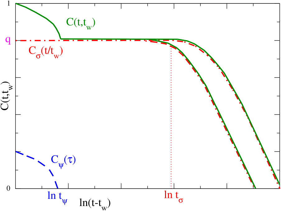
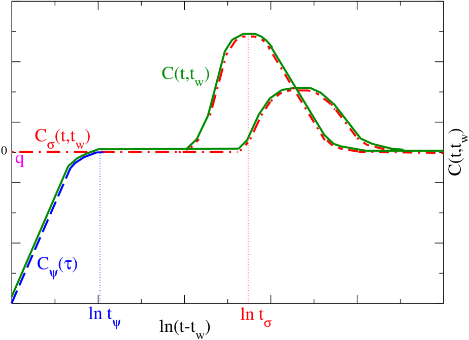
Figure 1: The behavior of $C_{\psi}(\tau)$, $C_{\sigma}(t,t_{w})$ and $C(t,t_{w})$, as $\tau=t-t_{w}$ is varied, is schematically shown on a log-log plot. The left panel is for a ferromagnetic system, the right one for the urn model. For each function two waiting times are considered, the curves corresponding to the larger $t_{w}$ decay later (the curves for $C_{\psi}$ collapse on a single one because this quantity is stationary). Note that, as discussed in the text, for a ferromagnet $C_{\sigma}(t,t_{w})$ only depends on $t/t_{w}$.

Conversely, letting again $t_{w}\to\infty$ but keeping $t/t_{w}$ (or the ratio $\ell(t)/\ell(t_{w})$, where $\ell$ is a monotonously increasing function, in specific systems) finite, one has $\tau\sim t_{w}\sim t_{\sigma}$: This means that the analysis is focused on the timescale of the slow (or aging) components. In this time sector, usually denoted as aging regime (on the right side of the left panel of of Fig. 1), the fast degrees act as a stationary background and the time evolution of the slow modes is probed. Indeed, from $\tau\simeq t_{\sigma}$ onward also ${\cal O}_{\sigma}$ starts changing and ${\cal O}$ moves from the plateau ${\cal O}(t,t_{w})\simeq q$ to the final value $\lim_{\tau\to\infty}{\cal O}(t,t_{w})$.

Generally, a good separation of the degrees can only be operated for very large times. The previous discussion shows that, in this case, two-time observables are quantities particularly fitted to highlight the role played by $\psi$ and $\sigma$.

We mentioned before that $\lim_{t\to\infty}{\cal O}_{\sigma}=0$ occurs for sufficiently regular observables ${\cal O}$. We now precise this point. Consider, in order to keep the discussion simple, a quantity that can be expressed as ${\cal O}=\sum_{i}o^{(i)}$, where the index $i$ runs over the microscopic degrees of freedom and $o^{(i)}$ is the contribution of one such degree. This is usually the case when dealing with extensive quantities. Then we can write ${\cal O}_{\sigma}(t)=\sum_{i\in\{\sigma\}}o_{\sigma}^{(i)}(t)=n_{\sigma}(t)\overline{o}_{\sigma}(t)$, where $\overline{o}_{\sigma}(t)$ is the average contribution to ${\cal O}_{\sigma}$ provided by one slow degree. If the time-dependence of $\overline{o}_{\sigma}(t)$ is such that $\lim_{t\to\infty}n_{\sigma}(t)\overline{o}_{\sigma}(t)=0$, then $\lim_{t\to\infty}{\cal O}(t)=\lim_{t\to\infty}{\cal O}_{\psi}(t)={\cal O}_{eq}$ and we call ${\cal O}$ an equilibrating quantity. Otherwise, the contribution of ${\cal O}_{\sigma}$ does not disappear and $\lim_{t\to\infty}{\cal O}\neq{\cal O}_{eq}$.

Depending on the system considered and on the nature of ${\cal O}$ either situation can be observed. In most cases $\overline{o}$ is weakly dependent on time, and the corresponding observable is an equilibrating one. For instance the energy of a non-disordered magnet quenched to a temperature $T_{f}$ below the critical temperature converges to the value $E_{eq}(T_{f})$ provided by the standard equilibrium statistical mechanical calculation. However there are also some notable exceptions, as for instance the response function $\chi(t)$ (a quantity deeply related to the magnetic energy) of a disordered one-dimensional magnet quenched to $T_{f}=0$, as described by the Ising chain with a random magnetic field of strength $h$. In the limit $h\to 0$ one finds [13, 14, 15, 16, 17] $\lim_{t\to\infty}\chi(t)\neq\chi_{eq}$.

3 Identification of stationary and aging modes

A possible identification of fast and slow degrees, based on arguments similar to the ones discussed in the previous section, can be given along the lines of Ref. [8]. Referring to a system described by a collection $S_{i}=\pm 1$ of spin variables one defines the slow part of $S_{i}$ in terms of the running time-average

$$\sigma_{i}(t)\simeq\frac{1}{\Delta t}\int_{t}^{t+\Delta t}dz\,S_{i}(z)$$ (4)

where

$$t_{\psi}\ll\Delta t\ll t_{\sigma}.$$ (5)

The fast part is then obtained by subtraction

$$\psi_{i}\simeq S_{i}(t)-\sigma_{i}(t).$$ (6)

The idea in Eq. (4) is that, since $\Delta t$ is chosen much larger than $t_{\psi}$ the contribution to $S_{i}$ of the fast modes self-averages to zero (in a more general situation the fast degrees may average to a finite constant value) and we are left precisely with the contribution of the slow modes.

The condition $\Delta t\ll t_{\sigma}$ guarantees that the slow modes are frozen on the timescale $\Delta t$, therefore the running average in Eq. (4) does not mix its value at time $t$ with the future evolution.

Clearly, as it is, Eq. (4) is tautological since we usually don’t know $t_{\sigma}$ unless the slow degrees are defined. However, using the properties of two-time quantities described in Sec. 2 and sketched in the left panel of Fig. 1, the condition (5) can be translated into

$$\frac{1}{\Delta t}\int_{t}^{t+\Delta t}C(z,t_{w})\,dz\simeq C(t+\Delta t,t_{w})$$ (7)

or equivalently

$$\frac{1}{\Delta t}\int_{t_{w}-\Delta t}^{t_{w}}C(t,z)\,dz\simeq C(t,t_{w}-\Delta t),$$ (8)

for the autocorrelation function

$$C(t,t_{w})=\langle S_{i}(t)S_{i}(t_{w})\rangle.$$ (9)

This can be understood looking at the schematic plot on the left panel of Fig. 1. Indeed, let us consider the three possible choices of $t$: i) $t_{w}<t<t_{w}+t_{\psi}$, ii) $t_{w}+t_{\psi}<t<t_{w}+t_{\sigma}$ and iii) $t>t_{w}+t_{\sigma}$. Starting from ii), in this case the correlation function is constant and equal to $q$ (to be precise this occurs if $t_{w}+t_{\psi}<t<t_{w}+t_{\sigma}-\Delta t$ but $t_{w}+t_{\sigma}-\Delta t\simeq t_{w}+t_{\sigma}$ because of (5)) and therefore equations (7) and (8) are obvious. On the other hand, considering for simplicity Eq. (7) (for Eq. (8) one can proceed similarly), in case i) $C(z,t_{w})$ is not a constant in the interval $z\in[t_{w},t_{w}+t_{\psi}]$ but this integration interval is negligible if the condition $\Delta t\gg t_{\psi}$ in Eq. (5) is met. Finally, Eq. (7) is true also in the last case iii), because in this stage $C$ is decreasing but this occurs on timescales of order $t_{\sigma}$, while we have chosen $\Delta t\ll t_{\sigma}$.

Letting $t_{w}=t$ in Eq. (7), with $t$ chosen as in ii) above, one has

$$C(t+\Delta t,t)\simeq q,$$ (10)

which very transparently appears as a direct manifestation of the choice (5). The quantity $q$ in this case amounts to the so-called Edwards–Anderson order parameter. In the previous argument and in what follows it is understood that the symbol $\simeq$ is correct in the large-$t_{w}$ limit, and the corresponding equalities become exact (i.e. with $\simeq$ replaced by a strict equality $=$) for $t_{w}\to\infty$.

Let us notice that the modes $\sigma_{i},\psi_{i}$ defined through Eqs. (4,6) are statistically independent. Indeed any cross-correlation between them vanishes

$$\langle\sigma_{i}(t)\psi_{i}(t_{w})\rangle=\langle\psi_{i}(t)\sigma_{i}(t_{w})\rangle=0,$$ (11)

as can be easily proved

$$\langle\sigma_{i}(t)\psi_{i}(t_{w})\rangle =\langle\sigma_{i}(t)\left[S_{i}(t_{w})-\sigma_{i}(t_{w})\right]\rangle$$

$$=\frac{1}{\Delta t}\int_{t}^{t+\Delta t}C(z,t_{w})dz-\frac{1}{(\Delta t)^{2}}\int_{t}^{t+\Delta t}\int_{t_{w}-\Delta t}^{t_{w}}C(z,y)dzdy$$

$$\simeq C(t+\Delta t,t_{w})-C(t+\Delta t,t_{w}-\Delta t)\simeq 0,$$ (12)

where we have used Eqs. (7,8) and the last passage can be obtaind by reasoning as below Eq. (9) enforcing the properties of $C$. The second relation in (11), namely $\langle\psi_{i}(t)\sigma_{i}(t_{w})\rangle=0$, can be proved analogously.

Due to the statistical independence (11), the correlation splits into

$$C(t,t_{w})=C_{\psi}(\tau)+C_{\sigma}(t,t_{w}),$$ (13)

where we have assumed that the $\psi_{i}$’s are stationary variables. The schematic behavior of $C_{\psi}$ and $C_{\sigma}$ is shown in the left panel of Fig. 1.

While $\mathcal{O}_{\psi}$ inherits the properties of the target equilibrium state, the aging part $\mathcal{O}_{\sigma}$ displays new features characteristic of non-equilibrium, as a remarkable gauge invariance called dynamical scaling. This can be expressed as the fact that the flow of time can be fully taken into account by changing the units $\ell$ of measure of certain dimensional physical quantities. Assuming, as it usually (but not necessarily) is, these to be lengths, one has invariant forms by measuring lengths in unit of the time-dependent unit of measure $\ell(t)$. For instance, in ferromagnets the equal-time correlation function $G(r,t)=\langle S_{i}(t)S_{j}(t)\rangle$ between spins $i,j$ at distance $r$ obeys

$$G_{\sigma}(r,t)=\hat{g}\left[\frac{r}{\ell(t)}\right],$$ (14)

where $\hat{g}$ is a scaling function. The clear meaning of this is that configurations of the same system at different times look the same on average if we rescale space by the characteristic unit measure of lengths, which in this case has the very transparent meaning of the size of the growing ordered domains of the two symmetry related equilibrium phases at $T=T_{f}$. More generally, for a one-time quantity which depends on space, scaling implies

$${\cal O}_{\sigma}(r,t)=\ell^{-b}(t)\,\hat{o}\left[\frac{r}{\ell(t)}\right],$$ (15)

Eq. (14) being a particular case with $b=0$.

In a similar way, for the autocorrelation of a ferromagnet one has $C_{\sigma}(t,t_{w})=\hat{c}\left[\frac{\ell(t)}{\ell(t_{w})}\right]$ which is a particular case (again with $b=0$) of the general scaling

$${\cal O}_{\sigma}(t,t_{w})=\ell^{-b}(t_{w})\,\hat{o}\left[\frac{\ell(t)}{\ell(t_{w})}\right].$$ (16)

In ferromagnetic systems with a scalar order parameter, like those described by the Ising model, the two classes of degrees $\{\psi\},\{\sigma\}$ have a natural interpretation [18]. After a temperature quench domains of the two equilibrium phases with magnetization $\pm M$ form, compete and grow. In this case $\sigma_{i}$ and $\psi_{i}$ can be thought as the background magnetization of the domains, which goes from $+M$ to $-M$ passing from zero upon moving across a domain’s boundary, and the fast thermal flips of spins on top of this background, respectively.

Interestingly, a separation of degrees of freedom into two classes with well separated time-scales can be exhibited in an exactly solvable model describing a ferromagnetic system with a vectorial order-parameter with ${\cal N}$ components, in the large-${\cal N}$ limit [9]. The order parameter $\phi(\vec{x},t)$ – which can be viewed as a coarse-grained spin – can be explicitly decomposed as $\phi(\vec{x},t)=\psi(\vec{x},t)+\sigma(\vec{x},t)$ in an exact analytical way, and the statistical independence (11) is proved.

The previous considerations show that, in some cases, the splitting of the degrees can be achieved. However, in the previous examples the two kind of modes are spatially mixed because both components are uniformly spread around the whole system. In the rest of the paper, instead, we will concentrate on a simple aging system, the zeta urn model [10, 11, 12, 19, 20, 21, 22] which, besides the advantage of being analytically tractable, has the remarkable property that $\{\psi\}$ and $\{\sigma\}$ are segregated in different parts of the system. This allows to concretely visualize them and offers a more intuitive interpretation.

4 The zeta urn model

The zeta urn model is defined by a collection $r_{i}\in\{0,1,\dots,M\}$ of integer variables defined on a network of $N$ nodes $i$. Usually the nodes are identified as boxes or urns inside which $r_{i}$ marbles, whose number $M=\sum_{i=1}^{N}r_{i}$ is fixed and conserved, can be accommodated. A cost function, or Hamiltonian, is introduced as the sum of independent contributions from all the nodes

$${\cal H}(\{r_{i}\})=\sum_{i=1}^{N}E_{i},$$ (17)

where

$$E_{i}=\ln(r_{i}+1)$$ (18)

is the (energy) cost to accommodate $r_{i}$ marbles inside the $i$-th box. In a statistical mechanical approach one introduces a canonical ensemble at the inverse temperature $\beta$ and configurations $\{r_{i}\}$ are weighted by the Boltzmann measure

$${\cal P}(\{r_{i}\})=Z^{-1}(\beta,N,M)e^{-\beta{\cal H}(\{r_{i}\})}$$ (19)

where

$$Z(\beta,N,M)=\sum_{\{r_{i}\}}e^{-\beta{\cal H}(\{r_{i}\})}$$ (20)

is the partition function. An exact computation shows the existence of a density-dependent critical temperature $T_{c}=\beta_{c}^{-1}$. Above such temperature the probability $P(r)$ of any of the identical urns to contain $r$ marbles decays exponentially with $r$, while

$$P(r)\sim(r+1)^{-\beta},$$ (21)

with $\beta=\beta_{c}$, at the critical point. In the low-temperature phase a macroscopic condensate appears: the occupation probability $P(r)$ is still given by Eq. (21), with the current value of $\beta$, for all the boxes except one, which contains an extensive number of marbles.

The equilibrium measure is invariant under a dynamics that respects detailed balance. In the following we will consider a kinetic rule where the number of particles is conserved and the transition rate $w(r_{i},r_{j})$ to move a particle from a non-empty urn $i$ to another $j$, chosen randomly in the network and containing respectively $r_{i}$ and $r_{j}$ particles before the move, is given by the Metropolis expression

$$w(r_{i},r_{j})=\min\left[1,\exp(-\beta\Delta E)\right],$$ (22)

where

$$\Delta E=\ln(r_{i})-\ln(r_{i}+1)+\ln(r_{j}+2)-\ln(r_{j}+1)$$ (23)

is the variation of the energy due to the move. Notice that the present kinetic rule has a mean field nature, in the sense that particles can be transferred between any couple of nodes.

The dynamics of the present model was solved exactly in different conditions in Ref. [22] where many quantities were computed. Here, since we are interested in separating degrees of freedom with different properties, we study it numerically.

5 Numerical study of the model

We performed a series of simulations of a system of $N=500$ urns, which are initially prepared in an infinite temperature equilibrium condition with particles distributed according to

$$P(r)=\frac{\rho^{r}}{(\rho+1)^{r+1}},$$ (24)

where $\rho=M/N$ is the density which, in the following, we will set to $\rho=2$. From this initial condition we quench the system to the final inverse temperature $\beta_{f}=(k_{B}T_{f})^{-1}=6>\beta_{c}$, meaning that we evolve the dynamics with this value of $\beta$ in the transition rates (22). Observables are averaged over a non-equilibrium ensemble of $3\times 10^{5}$ realizations of the process with different initial conditions and thermal histories.

The target equilibrium state with a macroscopic number of marbles condensed in a single urn is approached by a dynamical process that can be roughly divided into three stages. In an early stage, for $0<t\ll N$ (where $t$ is the time elapsed after the quench, measured in units of Monte Carlo sweeps), a segregation occurs between urns with a low occupation number, that we will denote as the gas phase in the following, and a liquid phase containing boxes occupied by many marbles. For larger times $N\ll t\ll N^{2}$ a scaling regime sets in during which the gaseous regions remain on average stationary while urns of the liquid phase compete and, as an effect of this, their number diminishes. Eventually, for $t\gg N^{2}$ a finite-size effect sets in, the symmetry between the nodes is spontaneously broken, a finite fraction of marbles is stored in a prevailing urn and the rest of them is dispersed among the remaining $N-1$ boxes.

5.1 Occupation probability

This whole pattern of behavior is mirrored by the evolution of the occupation probability $P(r,t)$, as it is shown in Fig. 2. From the initial distribution, $P(r,t)$ starts to progressively form a hollow at an intermediate value $r_{min}$ of $r$, signalling that the segregation process is started, and around $t\simeq 10^{2}$ a secondary peak is developed around $r=r_{max}=10$. From this time onward the peak moves progressively to larger values of $r$ and becomes more pronounced as compared to the hollow minimum. We will say that urns with $r<r_{min}$ are in the gaseous phase and the remaining ones in the liquid one.

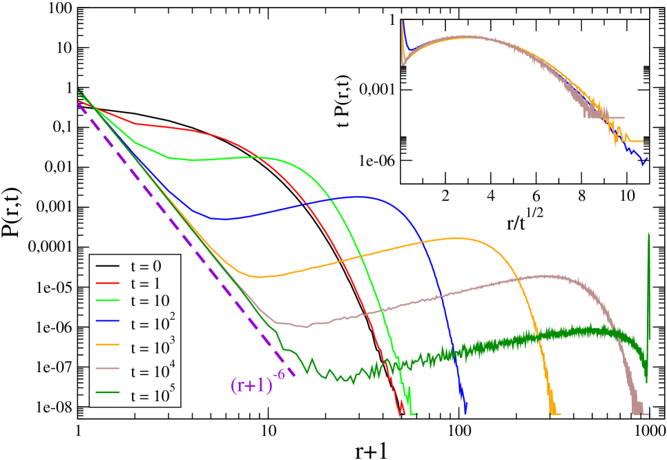
Figure 2: The occupation probability $P(r,t)$ is plotted against $r+1$ on a log-log plot for $\beta_{f}=6$ and $\rho=2$. The dashed violet line is the law $(r+1)^{-6}$, namely the equilibrium occupation probability (21) of the target equilibrium state. In the inset $t\,P(r,t)$ is plotted against $r/t^{1/2}$.

Around $t\simeq t_{sc}\simeq 1.5\cdot 10^{2}$ the second regime is entered, where the form of the different curves do not seem to change except for a rescaling of both axis.

Eventually, around $t=10^{5}$ a sharp peak located at the upper right of the spectrum starts growing. This is the hallmark of the final stage of the process where the finite size is felt and all the condensed marbles fill a single urn.

In the following we will concentrate on the second regime where the scaling properties are observed. Let us stress that, if the thermodynamic limit $N\to\infty$ (with fixed $\rho$) is taken from the onset, this stage becomes truly asymptotic. As discussed in Secs. 1, 2, 3, this is the regime where the two classes of degrees $\{\psi\}$ and $\{\sigma\}$ coexist.

We show now that these two sets can be consistently associated to the gaseous and the liquid urns. In order to do that, we observe that – as it can be seen in Fig. 2 – for $r<r_{min}$ the curves are time-independent and all collapse on the equilibrium power-law distribution (21). Therefore urns with $r\ll r_{min}$ are already in an equilibrium state and this is the characteristic property of the $\{\psi\}$ component. Conversely – as it is shown in the inset of Fig. 2 – by plotting $t\,P(r,t)$ vs $r/t^{1/2}$, for $r\gg r_{min}$ the curves at different times collapse on a single master curve. This means that the form

$$P_{\sigma}(r,t)=\ell^{-2}(t)\,\hat{p}\left(\frac{r}{\ell(t)}\right)$$ (25)

is obeyed, where [19]

$$\ell(t)=t^{1/2}$$ (26)

is a time-dependent characteristic marble number and $\hat{p}$ is a scaling function.

Equation (25) is a typical scaling property, formally identical to Eq. (15), with the difference that $r$ is not a space coordinate but, say, the height of the stack of marbles in an urn and $\ell(t)$ the unit to measure it. This suggests the quite natural identification of the highly populated urns with $r>r_{min}$ as $\{\sigma\}$ (hence the subscript in $P_{\sigma}$). Notice that the property (25) implies that the number $n_{\sigma}(t)\simeq\sum_{r=r_{min}}^{N}P(r,t)$ of liquid urns decreases as

$$n_{\sigma}(t)\sim\ell(t)^{-1}\,,$$ (27)

as it is expected for an aging component according to Eq. (1). Since the number of marbles in the condensate is roughly constant during the scaling regime, the shrinking of $n_{\sigma}(t)$ entails a correspondent growth of the occupation number of a liquid urn proportional to $\ell(t)$. This justifies the physical interpretation of $\ell(t)$ as the natural unit of measure of $r$.

The scaling (25) implies also that $\lim_{t\to\infty}P_{\sigma}(r,t)=0$, that is the property (3), hence $P(r,t)$ is an equilibrating quantity. However quantities like the fluctuation $\langle r^{2}\rangle_{\sigma}-\langle r\rangle_{\sigma}^{2}$ of the number of liquid marbles (where $\langle r\rangle_{\sigma}=\sum_{\sigma}r\,P(r,t)$ and similarly for $\langle r^{2}\rangle_{\sigma}$) are not equilibrating, as it can easily be checked using Eq. (25).

5.2 Energy

As a different example of a one-time quantity we have considered the energy density $\varepsilon(t)=E(t)/N=\langle{\cal H}\rangle/N$ of the system, where the Hamiltonian is given in Eq. (17). Following the decomposition (2) we write $\varepsilon(t)=\varepsilon_{\psi}(t)+\varepsilon_{\sigma}(t)$ and, using the non-interacting character (17) of the model, we define $\varepsilon_{\psi}=\sum_{i\in\{\psi\}}E_{i}/N$ and $\varepsilon_{\sigma}=\sum_{i\in\{\sigma\}}E_{i}/N$ (the two sets $\{\psi\}$ and $\{\sigma\}$ are identified as discussed above). These quantities are shown in Fig. 3. $\varepsilon_{\psi}(t)$ converges to the final equilibrium value $\varepsilon_{eq}(T_{f})=-\zeta^{\prime}(\beta)/\zeta(\beta)$ in a time of order $t\simeq 10^{3}$. $\varepsilon_{\sigma}(t)$ decays to zero proportionally to $(\ln t)/\sqrt{t}$, as can be checked using the scaling form (25), showing that the internal energy is an equilibrating quantity and that, for large time, the contribution of $\varepsilon_{\sigma}$ can be neglected in $\varepsilon$.

Notice that the property $\lim_{t\to\infty}\varepsilon_{\psi}(t)=\varepsilon_{eq}(T_{f})$ is an independent confirmation of the reliability of the method proposed above to separate fast and slow degrees.

We have also computed the variance $\Sigma(t)=\langle{\cal H}^{2}\rangle-\langle{\cal H}\rangle^{2}$ of the energy and of its gaseous and liquid parts, $\Sigma_{\psi}(t)=\langle{\cal H}^{2}\rangle_{\psi}-\langle{\cal H}\rangle_{\psi}^{2}$ and $\Sigma_{\sigma}(t)=\langle{\cal H}^{2}\rangle_{\sigma}-\langle{\cal H}\rangle_{\sigma}^{2}$, respectively. These quantities are shown in the inset of Fig. 3. Here one sees that for sufficiently long times ($t\gtrsim 500$), when the separation of degrees becomes effective, $\Sigma(t)=\Sigma_{\psi}(t)+\Sigma_{\sigma}(t)$. This is a nice indication that the $\psi$’s and the $\sigma$’s are statistically independent variables.

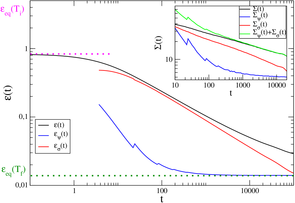
Figure 3: The quantities $\varepsilon(t)$, $\varepsilon_{\psi}(t)$ and $\varepsilon_{\sigma}(t)$ are plotted against $t$ in a double logarithmic plot. The dashed lines are the analytically known equilibrium values $\varepsilon_{eq}(T_{i})$ and $\varepsilon_{eq}(T_{f})$ at the initial and final temperatures, respectively. In the inset the variances $\Sigma(t)$, $\Sigma_{\psi}(t)$, $\Sigma_{\sigma}(t)$ are shown together with the sum of the last two.

5.3 Autocorrelation function

As an example of two-time quantity we consider the autocorrelation function. The number-number correlation

$$\widetilde{C}(t,t_{w})=\langle r_{i}(t)r_{i}(t_{w})\rangle-\rho^{2},$$ (28)

which does not depend on $i$ due to homogeneity, was analytically worked out in [22]. However this quantity is not well suited to the purposes of our paper because it is entirely dominated by the contribution of the highly populated urns forming the condensate. For this reason, instead of $\widetilde{C}$, we will consider

$$C(t,t_{w})=\langle\delta r_{i}(t)\delta r_{i}(t_{w})\rangle,$$ (29)

where $\delta r_{i}(t)=r_{i}(t+1)-r_{i}(t)$, is the variation of the number of marbles in the $i$-th urn. This quantity is related to $\widetilde{C}$ by

$$C(t,t_{w})=\widetilde{C}(t+1,t_{w}+1)-\widetilde{C}(t+1,t_{w})-\widetilde{C}(t,t_{w}+1)+\widetilde{C}(t,t_{w}).$$ (30)

The definition (29) is inspired by the autocorrelation encountered in the study of ferromagnetic systems. Typical values taken by the $\delta r$’s are $\delta r_{i}(t)=0,\pm 1$ (any value between $-M$ and $M$ is in principle possible, but with a very small probability) for all the urns, and this makes the difference with the definition (28) where the largest contribution is provided by large values of $r_{i}$ from the urns in the liquid phase.

Let us now discuss the splitting (13) of this autocorrelation. The gaseous part $C_{\psi}$ has very different features with respect to the liquid one $C_{\sigma}$. If an urn is in the gas phase, the number of marbles contained in it fluctuates rapidly around the average gas occupation number $\rho_{c}=\zeta(\beta-1)/\zeta(\beta)-1\simeq 0.019$ (where $\zeta$ is the Riemann’s zeta-function), hence $C_{\psi}$ is expected to converge quite rapidly (over a microscopic typical time of the equilibrium state) to zero. This decay occurs from the negative side, because if by chance an urn with an average number of balls receives an extra marble, it will most probably release it in the future in order to keep its occupation number close to the mean. Furthermore, on general grounds, $C_{\psi}$ is expected to depend only on the time difference $\tau$.

Conversely, in the effort to build the condensate, one urn in the liquid phase have the tendency to increase its number of marbles. This occurs up to a long time (of order $t_{w}$) when the competition with another prevailing urn will become effective and it will be progressively depleted. As a consequence, $C_{\sigma}$ is expected to show a pronounced maximum at a time monotonously increasing with $t_{w}$ and then to decrease to zero.

All these features are clearly displayed in the main part of Fig. 4, where the autocorrelation is plotted against $t-t_{w}$ for different values of $t_{w}$. Let us start by considering the solid green lines, which correspond to the whole correlation $C(t,t_{w})$.

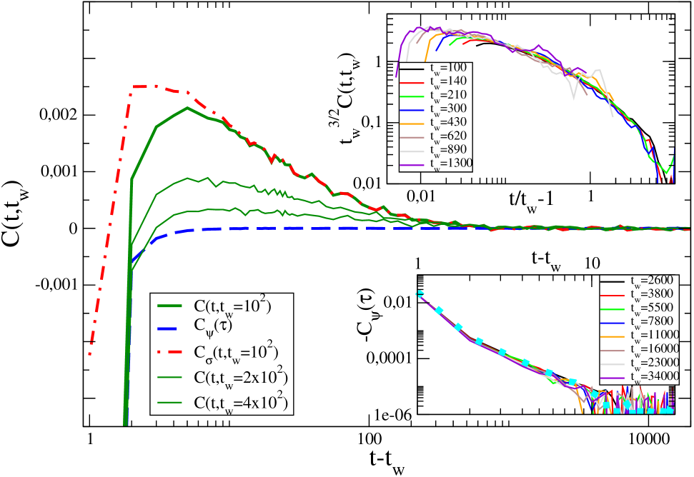
Figure 4: The autocorrelation $C(t,t_{w})$ (continuous green curves) is plotted against $t-t_{w}$ on a semi-log scale, for three different waiting times (lower curves correspond to larger $t_{w}$). The long-dashed blue curve is $C_{\psi}(\tau)$ and the dot-dashed red one is $C_{\sigma}(t,t_{w})$. In the upper inset the data collapse of the same curves of the left panel is obtained by plotting $t_{w}^{3/2}C(t,t_{w})$ against $(t-t_{w})/t_{w}$. In the lower inset $-C_{\psi}(t,t_{w})$ is plotted for different choices of $t_{w}$ (see key). The cyan dots denote $-C_{eq}(\tau)$.

The curves relative to different values of $t_{w}$ collapse for short times, up to $t-t_{w}\simeq 2$. In this regime $C(t,t_{w})$ is negative. What we are observing in this region is clearly the evolution of the fast part $C_{\psi}(\tau)$.

From $t-t_{w}\simeq 2$ onward the curves grow to a positive maximum, which is delayed and suppressed as $t_{w}$ is increased, and then decrease to zero. This is the behavior expected qualitatively for $C_{\sigma}$. Furthermore, in this regime the curves for different $t_{w}$ can be collapsed by plotting $t_{w}^{3/2}C(t,t_{w})$, against $t/t_{w}$, as it can be seen in the inset of Fig. 4. This means that the scaling form

$$C(t,t_{w})\simeq\ell^{-3}(t_{w})\,\hat{c}\left(\frac{t}{t_{w}}\right)$$ (31)

is obeyed, which is of the expected type (16), with the behavior (26) of $\ell$ previously found and $b=3$, yet another consequence of the decrease (27) of urns in the liquid phase.

Let us mention that the form (31) is in agreement with the known behavior

$$\widetilde{C}(t,t_{w})=(\rho-\rho_{c})\,t_{w}^{1/2}\,\Phi(t/t_{w}),$$ (32)

(where $\Phi(x)$ is a scaling function) of $\widetilde{C}(t,t_{w})$ in the aging regime. Indeed, by plugging this expression into Eq. (30) and expanding for large $t_{w}$ the various correlations on the r.h.s. around the value $(t,t_{w})$ of their arguments, one finds Eq. (31) with $\hat{c}=-\frac{\rho-\rho_{c}}{2}\,\Phi^{\prime}(t/t_{w})$, where $\Phi^{\prime}(x)=d\Phi(x)/dx$.

In order to check the decomposition (13) we have separated the urns into the gaseous and the liquid phase as discussed previously, and we have separately computed $C_{\psi}$ and $C_{\sigma}$ by correlating among them degrees that pertain to one or the other set both at $t_{w}$ and $t$. These quantities are also plotted in Fig. 4, where it is seen that they reproduce the whole quantity $C$ in the short-time ($C_{\psi}$) and in the long-time regime ($C_{\sigma}$), respectively. For $C_{\sigma}$ we have also checked that the scaling (31) is obeyed.

In order to better compare the behavior of the autocorrelation in the present urn model with that of a ferromagnet we have represented it pictorially in the right panel of Fig. 1 using the same line styles and colors in the two cases. The analysis of the two panels shows that a similar scenario occurs, apart of course from the different functional form of the various correlations.

According to the general paradigm discussed in Sections 1, 2, 3, $C_{\psi}(\tau)$ should correspond to the correlation function of the target equilibrium state. In the lower inset of Fig. 4 we plot this quantity computed in the aging regime by separating the degrees of freedom for different choices of $t_{w}$. The data do not show any systematic dependence on $t_{w}$, confirming that our definition of the set $\{\psi\}$ has the expected stationary property. In order to compare $C_{\psi}$ with the equilibrium autocorrelation we have computed the latter numerically: An efficient way to equilibrate the system at $T<T_{c}$ is to break the urn symmetry by starting from an initial configuration with all the marbles in one urn. This avoids the aging regime caused by the competition among urns and allows the system to quickly reach the equilibrium state. The quantity $C_{eq}(\tau)$ measured in this way is shown in the lower inset of Fig. 4 with a heavy-dashed cyan curve. As expected, $C_{\psi}(\tau)$ and $C_{eq}(\tau)$ coincide within numerical errors. The equilibrium autocorrelation could also be computed analytically starting from the known [22] expression of $\widetilde{C}$

$$\widetilde{C}_{eq}(\tau)=A_{eq}(\beta_{f})\tau^{-(\beta-3)/2},$$ (33)

where $A_{eq}(\beta)$ is a temperature-dependent constant. From this it is trivial to derive the expression

$$C_{eq}(\tau)\simeq-\frac{(\beta-1)(\beta-3)}{4}A_{eq}(\beta_{f})\tau^{-(\beta+1)/2}$$ (34)

for $C_{eq}(\tau)$. We have checked that our numerical determination shown in the lower inset of Fig. 4 coincides within errors with Eq. (34).

Summarizing, our numerical data for the zeta urn model fit nicely in the general framework of slow relaxation discussed in Sections 1, 2, 3 if the degrees of freedom of the system – the occupation numbers $r_{i}$ – are divided into two sets $\{\psi\}$ and $\{\sigma\}$ according to the recipe described in Section 5.1.

Before closing this section, we briefly comment on the robustness of the overall picture with respect to different definitions – but same in spirit – of the fast and slow degrees. We tried to address this issue by changing the definition of $\psi$’s and $\sigma$’s and, next to the technique of Section 5.1, we have separated slow and fast degrees using the running average procedure Eqs. (4,6) of Section 3. More precisely, considering the autocorrelation function $C$ we have defined the slow part as

$$C_{\sigma}(t,t_{w})=\langle\Delta r_{i}(t)\Delta r_{i}(t_{w})\rangle$$ (35)

where $\Delta r_{i}(t)=(\Delta t)^{-1}[r_{i}(t+\Delta t)-r_{i}(t)]$ is the variation of number of marbles (normalized by $\Delta t$) in the $i$-th urn in a time $\Delta t$ such that – as discussed in Section 3 – $C_{\psi}(\tau=\Delta t)\simeq 0$. Inspection of Fig. 4 suggests $\Delta t\sim 10\div 50$ as reasonable values. By computing the quantity of Eq. (35) we found that, for sufficiently large values of $t-t_{w}$ the curve obtained superimposes on the determination of $C_{\sigma}$ obtained previously with the technique of Section 5.1. This results confirms the robustness of the degree-separation scenario.

6 Conclusions

In this paper we have discussed the paradigm of a simple class of aging systems where the dynamical properties can be accounted for by the coexistence of slow and fast degrees with different scaling properties.

We have studied – in particular – the kinetics of the zeta urn model following a quench from high temperature to a final one below the condensation temperature. This model is a useful playground where fast and slow degrees have an intuitive interpretation in terms of the occupation numbers of different urns, allowing a distinction between a gaseous and a liquid phase, corresponding to the two sets $\{\psi\}$ and $\{\sigma\}$ of fast and slow modes.

We have considered the behavior of one-time quantities, as the energy, and of two-time ones, specifically the autocorrelation function. Due to the progressive reduction of the measure of the aging set $\{\sigma\}$, one-time quantities rapidly attain the characteristic value of the final equilibrium state. Non-equilibrium features are better observed in two-time quantities where the gaseous and the liquid component can be evidenced by increasing the two times along particular directions in the $(t,t_{w})$ plane, namely focusing on the short-time or on the aging regime, very similarly to what is known for ferromagnetic or glassy spin systems.

The concept of an effective temperature is deeply related to the topic considered in the present Article. This quantity, which was originally introduced in the context of mean-field glass models [23, 24, 25, 26, 27], can be obtained from the relation between an autocorrelation function and the correspondent response function. For systems – like the one considered here – where two sets of degrees can be identified, one would expect two different temperatures associated to them. Accordingly, while the set $\{\psi\}$ is equilibrated at the bath temperature, a different effective temperature would characterize the slow part $\{\sigma\}$. An effective temperature for the zeta urn model based on the correlation (28) has already been investigated [22]: The different insight that could be provided by starting from our new definition (29) instead remains an open issue for future research.

References

- [1] Bouchaud JP, Cugliandolo LF, Kurchan J, Mezard M. Out of equilibrium dynamics in spin-glasses and other glassy systems, in Young AP (Ed.), Spin Glasses and Random Fields, World Scientific, Singapore, 1997.
- [2] Biroli G. A crash course on aging, 2005 (arXiv:cond-mat/0504681).
- [3] Cugliandolo LF. Dynamics of glassy systems, in Barrat J-L, Dalibard J, Kurchan J, Feigel’man MV (Eds.), Slow Relaxation and Nonequilibrium Dynamics in Condensed Matter, Les Houches - École d’Été de Physique Theorique, Vol. 77, Springer-Verlag, 2003 (arXiv:cond-mat/0210312).
- [4] Zannetti M. Aging in domain growth, in Puri S, Wadhawan V (Eds.), Kinetics of Phase Transitions, CRC Press, 2009 (arXiv:1412.4670).
- [5] Corberi F, Cugliandolo LF, Yoshino H. Growing length scales in aging systems, in Berthier L, Biroli G, Bouchaud J-P, Cipelletti L, van Saarloos W (Eds.), Dynamical heterogeneities in glasses, colloids, and granular media, Oxford University Press, 2010 (arXiv:1010.0149).
- [6] Henkel M, Pleimling M. Non-equilibrium phase transitions. Volume 2: Ageing and dynamical scaling far from equilibrium, Springer, Dordrecht, 2010.
- [7] Mazenko GF, Valls OT, Zannetti M. Field theory for growth kinetics. Phys. Rev. B 1988; 38(1): 520–542.
- [8] Franz S, Virasoro MA. J. Phys. A: Math. Gen. 2000; 33(5): 891–905.
- [9] Corberi F, Lippiello E, Zannetti M. Slow relaxation in the large- model for phase ordering. Phys. Rev. E 2002; 65: 046136.
- [10] Bialas P, Burda Z, Johnston D. Condensation in the Backgammon model. Nucl. Phys. B 1997; 493: 505–516.
- [11] Bialas P, Burda Z, Johnston D. Phase diagram of the mean field model of simplicial gravity. Nucl Phys B 1999; 542: 413–424.
- [12] Bialas P, Bogacz L, Burda Z, Johnston D. Finite size scaling of the balls in boxes model. Nucl Phys. B 2000; 575: 599–612.
- [13] Corberi F, de Candia A, Lippiello E, Zannetti M. Off-equilibrium response function in the one-dimensional random-field Ising model. Phys. Rev. E 2002; 65: 046114.
- [14] Corberi F, Lippiello E, Zannetti M. On the connection between off-equilibrium response and statics in non disordered coarsening systems. Eur. Phys. J. B 2001; 24: 359–376.
- [15] Corberi F, Lippiello E, Zannetti M. Interface fluctuations, bulk fluctuations, and dimensionality in the off-equilibrium response of coarsening systems. Phys. Rev. E 2001; 63: 061506.
- [16] Corberi F, Lippiello E, Zannetti M. Fluctuation dissipation relations far from equilibrium. J. Stat. Mech 2007; P07002.
- [17] Corberi F, Castellano C, Lippiello E, Zannetti M. Generic features of the fluctuation dissipation relation in coarsening systems. Phys. Rev. E 2004; 70: 017103.
- [18] Corberi F, Gonnella G, Piscitelli A. Heat exchanges in coarsening systems. J. Stat. Mech. 2011; P10022.
- [19] Drouffe J-M, Godrèche C, Camia F. A simple stochastic model for the dynamics of condensation. J. Phys. A: Math. Gen. 1998; 31(1): L19–L25.
- [20] Godrèche C. From urn models to zero-range processes: Statics and dynamics, in Henkel M, Pleimling M, Sanctuary R (Eds.), Ageing and the Glass Transition, Lect. Notes Phys. 716, Springer 2007.
- [21] Godrèche C, Luck JM. Nonequilibrium dynamics of urn models. J. Phys.: Condens. Matter 2002; 14(7): 1601–1615.
- [22] Godrèche C, Luck JM. Nonequilibrium dynamics of the zeta urn model. Eur. Phys. J B 2001; 23(4): 473–486.
- [23] Cugliandolo LF, Kurchan J. Analytical solution of the off-equilibrium dynamics of a long-range spin-glass model. Phys. Rev. Lett. 1993; 71(1): 173–176.
- [24] Cugliandolo LF, Kurchan J. On the out-of-equilibrium relaxation of the Sherrington–Kirkpatrick model. J. Phys. A: Math. Gen. 1994; 27(17): 5749–5772.
- [25] Crisanti A, Ritort F. Violation of the fluctuation–dissipation theorem in glassy systems: basic notions and the numerical evidence. J. Phys. A: Math. Gen. 2003; 36(21): R181–R290.
- [26] Cugliandolo LF, Kurchan J, Peliti L. Energy flow, partial equilibration, and effective temperatures in systems with slow dynamics. Phys Rev. E 1997; 55(4): 3898–3914.
- [27] Corberi F, Lippiello E, Zannetti M. The effective temperature in the quenching of coarsening systems to and to below . J. Stat. Mech. 2004; P12007.