Growing quantum states with topological order

Abstract

We discuss a protocol for growing states with topological order in interacting many-body systems using a sequence of flux quanta and particle insertion. We first consider a simple toy model, the superlattice Bose Hubbard model, to explain all required ingredients. Our protocol is then applied to fractional quantum Hall systems in both, continuum and lattice. We investigate in particular how the fidelity, with which a topologically ordered state can be grown, scales with increasing particle number $N$. For small systems exact diagonalization methods are used. To treat large systems with many particles, we introduce an effective model based on the composite fermion description of the fractional quantum Hall effect. This model also allows to take into account the effects of dispersive bands and edges in the system, which will be discussed in detail.

I Introduction

Since the discovery of the integer quantum Hall effect (IQHE) in 1980 Klitzing1980 and two years later the fractional quantum Hall effect (FQHE) Tsui1982, the interest in states exhibiting topological order has increased tremendously. Due to their robustness against local disorder, these states are for instance well suited for metrology Klitzing1980. Another interesting aspect of such interacting many-body systems is that they host states with anyonic excitations Arovas1984; Halperin1984; Moore1991. In this context, non-Abelian anyons are particularly exciting because they can be employed to build a topological quantum computer Nayak2008, if they can be coherently manipulated.

For many years, solid state systems with electrons appeared to be the only candidates to realize exotic many-body states, e.g. in the FQHE. However, their small intrinsic length scales make coherent control difficult. On the other hand, the rapid development of ultracold gases and photonic systems is a promising route to implement various Hamiltonians known from the solid state community, with full coherent control. With current state of the art technology, noninteracting topological states have been observed in ultracold gases Aidelsburger2013; Miyake2013; Jotzu2014; Aidelsburger2014 as well as photonic systems Hafezi2013; Rechtsman2013.

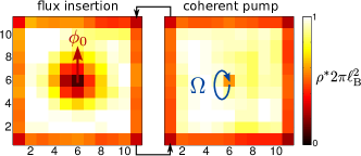
Figure 1: (Color online) Simulation of the effective composite fermion (CF) lattice model. The figure shows the CF density $\rho^{*}$ of a lattice with $11\times 11$ sites and effective flux per plaquette $\alpha^{*}=0.1$. The basic ingredients of the protocol are ($i$) flux insertion, which creates a CF quasi-hole excitation and ($ii$) a coherent CF pump, which refills the hole excitation. Additionally, we include a quasi-hole trapping potential ($g_{\mathrm{h}}=1J^{*}$) and absorbing boundaries ($\gamma_{\mathrm{Edge}}=0.0025J^{*}$) to account for the effects of dispersive bands and edge states.

Unlike in the solid state context, efficient cooling mechanisms below the many-body gap are still lacking in systems of interacting atoms and photons, which makes the preparation of topological states challenging. In this paper we develop an alternative dynamical scheme for the efficient preparation of highly correlated ground states with topological order. It can be implemented with ultracold atoms or photons and exploits the coherent control techniques available in these systems.

To solve the cooling problem, different approaches were discussed previously. In Umucalilar2012 it was suggested to pump the sites of a dissipative lattice system coherently. This scheme relies on a direct $N$-photon transition and thus works only for small systems. Moreover, the state prepared is in a superposition of different particle numbers. Another proposal Kapit2014 suggested to rapidly refill hole excitations due to local loss in a lattice system. This protocol stabilizes the ground state dynamically.

In reference Grusdt2014a, we proposed a scheme to grow the highly correlated Laughlin states. Here, we discuss the general ingredients of the protocol, which may also be used to grow other topological ordered states in interacting many-body systems. To do so, we consider a simple toy model explaining all necessary ingredients. The main ideas of the protocol can be summarized as follows. In the first step, a topologically protected and quantized Thouless pump Thouless1982 is used to create a localized hole excitation in the system. In the second step the hole is refilled using a coherent pump. Local repulsive interactions between the particles are employed to provide a blockade mechanism such that only a single particle is inserted. In the case of the FQHE, we analyze the performance of the protocol in detail and explain how the fidelity scales with the particle number $N$. In order to treat large fractional Chern insulator systems with many particles, we introduce an effective model based on the composite fermion (CF) description of the FQHE. Within this model, we are able to demonstrate, that the growing scheme still works despite the presence of gapless edge states and dispersive bands in large lattice systems. As shown in Fig. 1, we reach a homogeneous density in the bulk with an average CF magnetic filling factor $\nu^{*}\simeq 0.9$, close to the optimal value $\nu^{*}=1$.

The paper is structured as follows. We start by describing the growing scheme using a simple toy model in section II. In section III, we discuss the protocol in a FQH system. Moreover, we discuss the performance of the protocol. The last section IV considers fractional Chern insulators. There, we discuss edge and band dispersion effects based on our effective CF model.

II Topological growing scheme

In this section, we discuss the basic idea how states with topological order can be grown for the one dimensional superlattice Bose Hubbard model (SLBHM) as a toy model. This sets the stage for the following discussions of two dimensional systems with topological order.

II.1 Toy model

The SLBHM can be used to implement a quantized pump Berg2011; Thouless1982, which can be related to a nontrivial topological invariant. The Hamiltonian of the SLBHM is

$$\hat{\mathcal{H}}=-J_{1}\sum_{j}\hat{a}^{\dagger}_{j}\hat{b}_{j}+\text{h.c.}-J_{2}\sum_{j}\hat{a}^{\dagger}_{j}\hat{b}_{j+1}+\text{h.c.}\\ +\delta\sum_{j}\hat{b}^{\dagger}_{j}\hat{b}_{j}+U/2\sum_{j}\left(\hat{a}^{\dagger}_{j}\hat{a}^{\dagger}_{j}\hat{a}_{j}\hat{a}_{j}+\hat{b}^{\dagger}_{j}\hat{b}^{\dagger}_{j}\hat{b}_{j}\hat{b}_{j}\right),$$ (1)

where $\hat{a}_{j}(\hat{b}_{j})$ annihilates a boson on lattice site $A$ ($B$) in the $j$th unit cell (see Fig. 2a). Note, that we consider here a semi-infinite system with open boundary on the left. The hopping elements are denoted by $J_{1},J_{2}$, while $\delta$ is an onsite potential shift acting on lattice sites $B$. Furthermore, we include onsite interactions $U$ for more than one particle per site.

In the case of vanishing $\delta$ and disregarding interactions, the different hopping amplitudes $J_{1}\neq J_{2}$ determine the dimerization of the two sites $A$ and $B$ in the unit cell. This leads to a two-band model with a band gap $E_{\mathrm{gap}}$ and bandwidth $\Delta E$ determined by the ratio $J_{2}/J_{1}$. In the limit $J_{2}/J_{1}\rightarrow 0$ the flatness ratio $E_{\mathrm{gap}}/\Delta E$ tends to infinity and the two bands become nondispersive. At filling $\rho=1/2$ and with interactions, the ground state of the system is a Mott insulator (MI) with many-body gap $\Delta$ or a superfluid (SF) depending on the specific parameters $J_{2}/J_{1}$ and $U$ Buonsante2004; Buonsante2004a; Buonsante2005; Muth2008. Specifically, for large interactions $U$ the model can be mapped to free fermions. The resulting ground state at $\rho=1/2$ is incompressible whenever $J_{1}\neq J_{2}$ or $|\delta|\neq 0$. For finite interaction $U$, the SF region is extended in parameter space $(J_{1}-J_{2},\delta)$ as depicted in Fig. 2b.

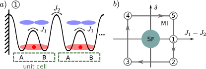
Figure 2: (Color online) (a) Semi-infinite chain of coupled dimers, consisting of two sites $A,B$. Initially, the MI ground state is prepared with filling $\rho=1/2$. (b) Schematic phase diagram of the SLBHM in the regime of intermediate interactions $U$. Following adiabatically the loop 1-5 corresponds to a Thouless pump: Encircling the SF region, all particles in the MI are shifted one dimer to the right.

II.2 Protocol

In the following, we illustrate the main steps of our growing scheme by showing how the MI ground state of this system can be grown. We note that there are more practical ways to prepare the ground state, of course, but the present protocol can be generalized to more complex systems, including states in the FQHE presented in section III and IV.

We will start to discuss the protocol in the nondispersive limit $J_{2}/J_{1}\rightarrow 0$, where hole excitations will remain localized. The effect of dispersive bands in the case of finite $J_{1}/J_{2}$ will be considered later. Let us assume, that the $N$ particle MI ground state of the SLBHM with filling $\rho=1/2$ is already prepared in a finite region of the lattice. We now show how the state with $N+1$ particles can be grown.

II.2.1 Topological pump

First, a topological Thouless pump Thouless1982 is used to create a hole excitation localized at the edge of the system. This process is related to Laughlin’s argument of flux insertion Laughlin1981 in the quantum Hall effect (QHE): Inserting one flux quantum $\phi_{0}$ leads to a quantized particle transport, which is the origin of the quantized Hall conductance $\sigma_{xy}$. In the SLBHM, the process of flux insertion is shown in Fig. 2b. By adiabatically changing the parameters $J_{1}-J_{2}$ and $\delta$ in time we encircle the critical SF region. After a full cycle of period $T_{\phi}$ all particles are shifted one dimer to the right, leaving a hole excitation on the left side of the system. The possibility to construct such a cyclic pump is deeply related to the underlying topological order of the model.

II.2.2 Coherent pump

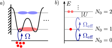
Figure 3: (Color online) (a) Coherent pump couples a reservoir of bosons to the left-most dimer. (b) Due to a blockade mechanism, only a single particle is pumped into the system. $\Omega_{\text{eff}}$ is the many-body Rabi-frequency, reduced by a Franck-Condon factor and $N_{0}$ the number of bosons in the left-most dimer.

In the following step, we replenish the hole excitation by a single boson. To this end, we coherently couple a reservoir of particles to the first lattice site of the system as shown in Fig. 3a. The coherent pump can be described by the Hamiltonian

$$\hat{\mathcal{H}}_{\Omega}=\Omega\hat{a}^{\dagger}_{0}\mathrm{e}^{-i\omega t}+\text{h.c.},$$ (2)

where $\Omega$ is the Rabi- and $\omega$ the driving frequency. The driving frequency $\omega$ is chosen to be resonant with the lowest band. Hence, if $|\Omega|$ is much smaller than the single-particle band gap $E_{\mathrm{gap}}$, particles can only be added in the lowest band. The corresponding Rabi-frequency $|\Omega_{\rm eff}|<|\Omega|$ is then however reduced by a Franck-Condon factor.

In general, the coherent pump (2) creates a coherent superposition state of $N_{0}$ bosons in the left-most Wannier orbital of the lowest band. To ensure that, at most, one boson is added, we employ a blockade mechanism, see Fig. 3b. For sufficiently strong interactions and weak enough driving,

$$U\gg|\Omega_{\rm eff}|$$ (3)

the transition to the $N_{0}=2$ particle state is detuned by the interaction energy $U$.

For $|\Omega_{\rm eff}|\ll\Delta$, at maximum one boson can be added into the lowest Bloch band. To replenish the hole excitation by precisely one boson at a time, one can use a $\pi$-pulse of duration $T_{\Omega}=\pi/2\Omega_{\text{eff}}$. Although the $\pi$-pulse is less robust to errors than e.g. an adiabatic sweep, we choose it because of its speed. This, we believe, is crucial to overcome linear losses present in realistic systems.

Starting from complete vacuum, the sequence described above can be repeated to grow the MI ground state with $N$ particles. Next, we discuss extensions of the protocol, required when the bands are dispersive or the system is finite.

II.2.3 Dispersive bands & finite systems

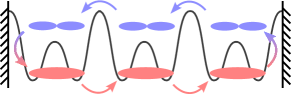
Figure 4: (Color online) Due to the process of flux insertion in a finite system, the higher band of the SLBHM will be occupied. While a state at the right edge of the system will be transferred into the upper band, a state from the left upper band, will be transferred to the lower band.

Dispersive bands $J_{1}/J_{2}\neq 0$ lead to intrinsic dynamics of the particles and thus of the hole excitations. The bandwidth $\Delta E$ of the lowest band sets the timescale for the dispersion. Firstly, the localized quasi-hole excitation created using the topological pump, disperses into the bulk of the system. Since the coherent pump couples locally to the left-most dimer, the hole cannot be refilled efficiently with a single boson. More importantly, the number fluctuations $\Delta N(t)=\left[\big{\langle}\hat{N}^{2}\big{\rangle}-\big{\langle}\hat{N}\big{\rangle}^{2}\right]/\big{\langle}\hat{N}\big{\rangle}$ will increase. To prevent the dynamics of the quasi-hole excitation, a quasi-hole trapping potential

$$\hat{\mathcal{H}}_{\mathrm{qh}}=g_{\mathrm{h}}\left(\hat{a}^{\dagger}_{0}\hat{a}_{0}+\hat{b}^{\dagger}_{0}\hat{b}_{0}\right)$$ (4)

acting on the left-most dimer can be used. The strength of the trap $g_{\mathrm{h}}$ should be weak enough not to destroy the topological order, but strong enough to trap the quasi-hole excitation. Concretely we require

$$\Delta E\lesssim g_{\rm h}\ll\Delta.$$ (5)

Secondly, the diffusion of bulk particles from the right edge of the system into vacuum lets the MI melt. Vice-versa, the diffusion of holes from the vacuum into the bulk at the right edge of the system makes the state compressible. For fast pump rates of the protocol, this effect can be neglected. However, if the bandwidth $\Delta E$ is the dominant contribution, we suggest to use a harmonic trapping potential. The potential should be weak enough to avoid localization effects (see Kolovsky2014). Therefore, in local density approximation, the bulk of the system will remain incompressible.

In finite systems with open boundaries, the flux insertion, as illustrated in Fig. 4, connects states from the lower and the upper band at the edges. As long as the upper band is empty, the topological pump creates a hole excitation in the lower band. However, once the right boundary is reached, particles will be excited to the upper band. To avoid the high energy excitations in the protocol, sufficiently strong losses $\gamma_{\mathrm{Edge}}$ localized at the right boundary of the system can be introduced.

III Fractional Quantum Hall States

We now apply the growing scheme to fractional quantum Hall (FQH) systems. In this case, the bands – i.e. Landau levels (LLs) – are nondispersive and we assume an infinite system.

III.1 Model

We consider a FQH model of bosons in the two dimensional disc geometry. The magnetic field can be implemented using e.g. artificial gauge fields. Moreover, we consider a contact interaction between the particles with strength $g_{0}$. In second quantized form, the Hamiltonian reads

$$\hat{\mathcal{H}}=\int\mathrm{d}^{2}\bm{r}\ \hat{\psi}^{\dagger}(\bm{r})\frac{1}{2M}\left(\bm{p}-\bm{A}\right)^{2}\hat{\psi}(\bm{r})\\ +\frac{1}{2}g_{0}\int\mathrm{d}^{2}\bm{r}\ \hat{\psi}^{\dagger}(\bm{r})\hat{\psi}^{\dagger}(\bm{r})\hat{\psi}(\bm{r})\hat{\psi}(\bm{r}),$$ (6)

where $\hat{\psi}^{\dagger}(\bm{r})$ creates a boson at the position $\bm{r}$. The first term in eqn. (6) includes the magnetic field in minimal coupling using the vector potential $\bm{A}=B/2(-y,x,0)$. In this symmetric gauge, the total angular momentum $L_{z}$ is a conserved quantity, $[\hat{\mathcal{H}},L_{z}]=0$.

For later purposes we express the field operators $\hat{\psi}(\bm{r})$ in terms of the bosonic operators $\hat{b}_{n,\ell}$ which create a particle in the orbital of the $n$th LL with angular momentum $\ell$. Here, $n$ and $\ell$ are integers with $n,\ell+n\geq 0$. We obtain

$$\hat{\psi}(\bm{r})=\sum_{n,\ell}\eta_{n,\ell}(\bm{r})\hat{b}_{n,\ell},$$ (7)

where $\eta_{n,\ell}(\bm{r})$ are the single particle wavefunctions, see e.g. Prange1987; Jain2007.

III.2 Laughlin States and Excitations - CF Picture

It was shown in Wilkin1998; Wilkin2000; Cooper1999; Regnault2003; Regnault2004, that the Laughlin (LN) wavefunction at magnetic filling $\nu=1/2$ is the exact zero energy ground state of the bosonic FQH Hamiltonian (6). The filling factor $\nu=N/N_{\phi}$ is defined as the ratio between particle number $N$ and number of flux quanta $N_{\phi}$. In terms of the complex coordinates $z_{j}=x_{j}-iy_{j}$ of the $j$th particle, the LN wavefunction is

$$|\text{LN},N\rangle\ \hat{=}\ \Psi_{\text{LN}}=\mathcal{N}_{\rm LN}\prod_{j<k}(z_{j}-z_{k})^{2}e^{-\sum_{j}|z_{j}|^{2}/4\ell_{\mathrm{B}}^{2}},$$ (8)

where $\mathcal{N}_{\rm LN}$ is a normalization constant. The magnetic length $\ell_{\mathrm{B}}=\sqrt{\hbar/B}$ depends only on the magnetic field $B$.

The zero energy excitations of the LN wavefunction are quasi-holes described by the wavefunction $\Psi_{\rm qh}=\mathcal{N}_{\rm qh}\prod_{j}z_{j}\Psi_{\rm LN}$. $m$ quasi-holes, located in the center, are described by the $m$ quasi-hole wavefunction

$$|m\text{qh},N\rangle\ \hat{=}\ \Psi_{m\text{qh}}=\mathcal{N}_{m\rm qh}\Big{(}\prod_{j}z_{j}\Big{)}^{m}\Psi_{\text{LN}}.$$ (9)

The LN state $|\text{LN},N\rangle$ and the quasi-hole state $|m\text{qh},N\rangle$ carry different total angular momentum $L_{z}$,

$$L_{z}\big{(}|\text{LN},N\rangle\big{)} =N(N-1)$$ (10)

$$L_{z}\big{(}|m\text{qh},N\rangle\big{)} =N(N-1)+mN.$$ (11)

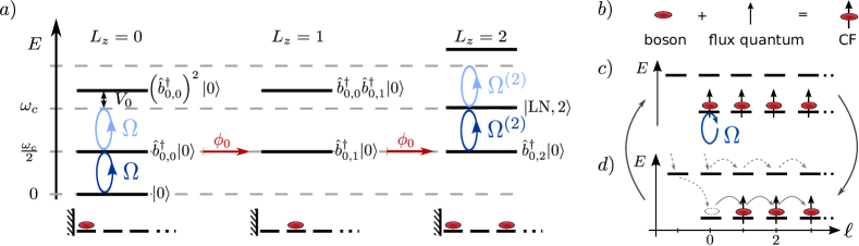
Figure 5: (Color online) (a) Growing scheme for the $\nu=1/2$ LN state in the continuum. The many-body eigenstates of the FQH Hamiltonian (6), between which transitions are driven, are shown as a function of the total conserved angular momentum $L_{z}$. Starting from the vacuum $|0\rangle$, the LN state with $N=2$ bosons is grown. After adding one boson in the central orbital, two flux quanta are adiabatically inserted and the resulting hole excitation is refilled by a second boson. This can be interpreted as replenishment of the system by a composite fermion, hence keeping intact the topological order of the system. The lowest line shows the schematics of the prepared states after every step. (Horizontal lines denote orbitals; This picture is valid in the thin-torus limit or after using the patterns as partitions determining certain Jack polynomials Bernevig2008.) (b) Flux attachment: A single boson together with one flux quantum form a CF. (c),(d) Level spectrum in terms of CFs. (c) Coherent pump process with Rabi-frequency $\Omega$. The lowest CF-LL is filled, corresponding to CF filling factor $\nu^{*}=1$. (d) Flux insertion process increases angular momentum $\ell$ by one.

Both wavefunctions can be understood in the more general framework of composite fermions (CFs) Zhang1989; Read1989; Jain1989; Jain2007. For the $\nu=1/2$ case, the LN wavefunction (8) can be decomposed into

$$\Psi_{\text{LN}}=\mathcal{N}_{\rm LN}\prod_{j<k}(z_{j}-z_{k})\Phi_{\mathrm{CF}}^{(\nu^{*}=1)}.$$ (12)

Besides the Jastrow factor $\prod_{j<k}(z_{j}-z_{k})$ attaching one flux quantum to each boson (see Fig. 5b), a fermionic wavefunction $\Phi_{\mathrm{CF}}^{(\nu^{*}=1)}$ appears. The Jastrow factor screens the interactions between the particles and leads to a reduced magnetic field $B^{*}=B/2$ seen by the CFs. As in the IQHE, their wavefunction is given by a Slater determinant of single particle orbitals filling the lowest CF-LL $\nu^{*}=1$, i.e. $\Phi_{\mathrm{CF}}^{(\nu^{*}=1)}=\prod_{j<k}(z_{j}-z_{k})\exp\left(-\sum_{j}|z_{j}|^{2}/4\ell_{\mathrm{B}}^{2}\right)$. The FQHE can be interpreted as an IQHE of noninteracting CFs in a reduced magnetic field $B^{*}$. The CF picture in the context of the FQHE is powerful in describing all fractions in the Jain sequence Jain1989 and moreover describes the quasi-hole excitations and their counting correctly. However, the CF theory does not reproduce the correct Laughlin gap $\Delta_{\text{LN}}$. Here, a microscopic theory of the full interacting many-body problem is necessary. Also in order to explain other than the main sequence of FQH states, interactions between CFs need to be taken into account.

III.3 Protocol

III.3.1 Topological pump – flux insertion

In the toy model II.1 we used a topological Thouless pump to shift the particles to the right. In the context of quantum Hall physics, this corresponds to Laughlin’s argument of flux insertion Laughlin1981, which was used to explain the quantization of the Hall conductivity. The idea is to insert locally in the center of the system flux quanta $\phi_{0}$ in time $T_{\phi}$, which produces an outwards Hall current $j_{r}\sim\mathrm{Ch}\ \partial_{t}\phi$ in radial direction. The quantization of the Hall current is related to the nontrivial Chern number $\mathrm{Ch}$ of the system. The process of inserting flux quanta increases the total angular momentum of the state. A more detailed discussion of the process in the noninteracting case can be found in appendix A.

Starting from the $\nu=1/2$ LN state $|\text{LN},N\rangle$ with $N$ particles, we insert two flux quanta $2\times\phi_{0}$ in time $T_{\phi}$ in the center of the system. In this way, we create a two-quasi-hole excitation $|2\text{qh},N\rangle$. The two-quasi-hole state $|2\text{qh},N\rangle$ already lies in the same angular momentum $L_{z}$ sector as the LN state $|\text{LN},N+1\rangle$ with $N+1$ particles (compare eqns. (10), (11)).

III.3.2 Coherent pump

In the next step, we refill the quasi-hole excitation using a coherent pump, which couples a reservoir of bosons to the hole excitation. As this is done in the center, no angular momentum is transferred. To this end, we supplement the FQH Hamiltonian (6) by a term

$$\hat{\mathcal{H}}_{\Omega}=\int\mathrm{d}^{2}\bm{r}\ g(t)\mathrm{e}^{-i\omega t}\delta^{2}(\bm{r})\hat{\psi}^{\dagger}(\bm{r})+\text{h.c.}$$ (13)

While $g(t)$ denotes the strength of the coherent pump, the driving frequency $\omega=\omega_{c}/2$ is chosen resonant with the lowest LL (LLL). In the regime of large magnetic fields and low temperatures, it is sufficient to project eqn. (13) to the LLL resulting in

$$\hat{\mathcal{P}}_{\text{LLL}}\hat{\mathcal{H}}_{\Omega}\hat{\mathcal{P}}_{\text{LLL}}=\Omega\mathrm{e}^{-i\omega t}\hat{b}^{\dagger}_{0,0}+\text{h.c.},$$ (14)

where we defined the Rabi-frequency $\Omega=g/\sqrt{2\pi\ell_{\mathrm{B}}^{2}}$. This corresponds to $\Omega_{\text{eff}}$ in the toy model.

Since the coherent pump does not change the angular momentum $L_{z}$ sector, we obtain a similar blockade mechanism as in the toy model (see Fig. 5a with $L_{z}=0,2$). In the corresponding sector, there is only one zero-interaction energy eigenstate, the $N+1$ LN state. The energy offset to any other states in the $(N+1)$-particle manifold is of the order of Haldanes zeroth pseudopotential $V_{0}$ Haldane1983. We require $\Omega\ll\omega_{c},V_{0}$ to avoid excitations to high energy states.

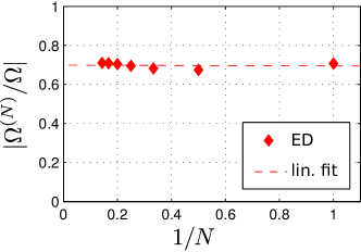
Figure 6: (Color online) Franck-Condon factors $\Omega^{(N)}/\Omega$, as defined in eqn. (15), for different particle numbers $N$ calculated using exact diagonalization (ED) in a system with contact interaction for up to $N=7$ particles. A linear fit is used to extrapolate $N\rightarrow\infty$.

To insert a single particle, we use a $\pi$-pulse of duration $T_{\Omega}=\pi/2\Omega^{(N)}$. Here, the bare Rabi-frequency $\Omega$ is reduced by a Franck-Condon factor

$$\Omega^{(N)}/\Omega=\langle\text{LN},N|\hat{b}^{\dagger}_{0,0}|2\text{qh},N-1\rangle,$$ (15)

which accounts for the overlap between the initial and final state. In Fig. 6 we show the Franck-Condon factors for different particle number $N$ and extrapolate to $N\rightarrow\infty$. To this end, we calculated the LN wavefunction using exact diagonalization . A linear fit suggests that even in the case $N\rightarrow\infty$ the Franck-Condon factor does not vanish with $\Omega^{(\infty)}/\Omega\simeq 0.7$.

III.3.3 CF picture

The first few steps of the protocol are illustrated in Fig. 5a. Another description of the protocol, which provides a much simpler physical picture uses the CF picture. Firstly, due to local flux insertion (see Fig. 5d), we generate a quasi-hole excitation. Secondly, the hole excitation is refilled by an effective coherent CF pump, for a particle together with one flux quantum. Analogously to the blockade mechanism, one CF refills the empty $\ell=0$ orbital (see Fig. 5c). By subsequent repetition, we grow the filling $\nu^{*}=1$ integer quantum Hall state of noninteracting CFs in a reduced magnetic field $B^{*}$.

The CF picture provides an explanation, why it is possible to grow highly correlated LN states. Since the CF wavefunction $\Phi_{\mathrm{CF}}^{(\nu^{*}=1)}$ is a separable Slater determinant of noninteracting CFs, we can grow the highly correlated LN state by adding CFs one by one to the system. Note that, although the wavefunction is a separable product state of CFs occupying Wannier functions (or Landau level orbitals), it has non-local topological order. This is because Wannier functions (or orbitals) of a single LL are non-local Brouder2007. On first glance, this may look contradicting as the dynamical growing scheme presented in this paper involves only local processes. However, the non-local topological order in the system is generated by the Thouless pump (flux insertion).

III.4 Performance

For interesting applications such as measuring the braiding statistics of elementary excitations, the LN state has to be prepared with high accuracy. To quantify the quality of the scheme, we calculate the fidelity $\mathcal{F}_{N}$ of being in the LN state with $N$ particles after $N$ steps of the protocol. The fidelity is defined as

$$\mathcal{F}_{N}=|\langle\Psi_{N}|\text{LN},N\rangle|,$$ (16)

where $|\Psi_{N}\rangle$ is the state after $N$ steps of the protocol. In the calculation of the fidelity $\mathcal{F}_{N}$ we include besides nonadiabatic transitions in the flux insertion and coherent pump process, a particle loss rate $\gamma$. This is important, since decay usually plays a crucial role, in particular in photonic systems.

The total time for a full cycle (flux insertion time $T_{\phi}$, coherent pump time $T_{\Omega}$) is $T=T_{\phi}+T_{\Omega}$. As will be discussed in detail later, we find for the fidelity perturbatively in the limit $\gamma T,(\Delta_{\text{LN}}T_{\phi})^{-1},(\Delta_{\text{LN}}T_{\Omega})^{-1}\ll 1$

$$\mathcal{F}_{N}\simeq\exp\left(-\frac{1}{2}N\left(\frac{1}{2}\gamma T(N+1)+\frac{\Lambda_{N}^{2}}{(\Delta_{\text{LN}}T)^{2}}\right)\right).$$ (17)

We see, that the losses and the nonadiabatic transitions contribute competitively in eqn. (17). While it is favorable to run the protocol as fast as possible to avoid losses, the adiabaticity requires long time scales $T$.

For fixed fidelity $\mathcal{F}_{N}=1-\varepsilon$, $\varepsilon\ll 1$, we calculate the maximal number of particles $N_{\mathrm{max}}$ which can be grown with optimal period $T_{\mathrm{opt}}$. To leading order in $N$, we approximately obtain

$$N_{\mathrm{max}} \simeq 1.365\varepsilon^{3/5}\left(\frac{\Delta_{\text{LN}}}{\Lambda_{N}\gamma}\right)^{2/5}$$ (18)

$$T_{\mathrm{opt}} \simeq 1.431\left(\varepsilon\gamma\right)^{-1/5}\left(\frac{\Lambda_{N}}{\Delta_{\text{LN}}}\right)^{4/5}.$$ (19)

The LN state with fildelity $\mathcal{F}_{N}=1-\varepsilon$ can be grown in time $T_{0}=N_{\mathrm{max}}T_{\mathrm{opt}}\sim N_{\mathrm{max}}^{3/2}\varepsilon^{-1/2}\Lambda_{N}/\Delta_{\text{LN}}$ scaling only slightly faster than linear with particle number $N_{\mathrm{max}}$. Note, that the fidelity decreases with increasing time $t>T_{0}$. In the following, we discuss the different contributions to the fidelity (17) in detail.

III.4.1 Loss

We assume a particle loss rate $\gamma\ll 1/T$, i.e. after one full period $T$ the probability of loosing a particle is small. The probability of a single decay process after $N$ steps of the protocol is then given by

$$P_{\gamma}=1-\exp\left(-\gamma T\sum_{n=1}^{N}n\right)\simeq\frac{1}{2}\gamma TN\left(N+1\right).$$ (20)

To leading order in $N$, the probability of loosing one particle increases quadratically with the particle number $N$.

III.4.2 Flux insertion

The process of flux insertion, as described in III.3, introduces one flux quantum $\phi_{0}$ in the center of the system. For simplicity, we assume the flux $\phi(t)=\phi_{0}\ t/T_{\phi}$ to change linear in time $t$. In the fully adiabatic protocol, the angular momentum $\ell$ is therefore increased by one without coupling different LLs $n,n^{\prime}$. We calculate in the noninteracting case the nonadiabatic coupling matrix element $\kappa=\langle n^{\prime},\ell|-i\partial_{\ell}|n,\ell\rangle$ between different LLs. To estimate the scaling of the probability $P_{\phi}$ for excitation of higher LLs, we consider the coupling between the LLs $n$ and $n+1$. In the regime of long times $T_{\phi}$, we determine $P_{\phi}$ perturbatively (see appendix B). Using the Laughlin gap $\Delta_{\text{LN}}$, we obtain

$$P_{\phi}\simeq\frac{\tilde{\kappa}^{2}}{(\Delta_{\text{LN}}T_{\phi})^{2}},$$ (21)

where $\tilde{\kappa}$ is a nonuniversal coupling constant. Importantly, nonadiabatic transitions to higher LLs scale as $\sim 1/(\Delta_{\text{LN}}T_{\phi})^{2}$.

III.4.3 Coherent pump

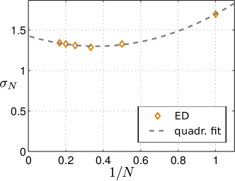
Figure 7: (Color online) Scaling of the nonuniversal factor $\sigma_{N}$ from eqn. (22) with particle number $N$. We interpolate $N\rightarrow\infty$ with a quadratic fit.

The coherent pump (14), as discussed in III.3, couples in zeroth order in $\Omega/\Delta_{\text{LN}}$ only the two-quasi-hole state $|2\text{qh},N\rangle$ to the Laughlin state $|\text{LN},N+1\rangle$. In first order perturbation theory, couplings to excited states in the $N-1,N,N+1,N+2$ particle sectors are relevant. We obtain for the probability of nonadiabatic excitations

$$P_{\Omega}\simeq\frac{\sigma_{N}^{2}}{(\Delta_{\text{LN}}T_{\Omega})^{2}},$$ (22)

where we used the $\pi$-pulse time $T_{\Omega}=\pi/2\Omega$. The nonuniversal factor $\sigma_{N}$ includes Franck-Condon factors and excitation energies $\Delta^{(N)}$ of undesired states weighted by the Laughlin gap $\Delta_{\text{LN}}$ (see appendix C). In Fig. 7 $\sigma_{N}$ is calculated for various particle numbers $N$ using exact diagonalization. For $N\rightarrow\infty$ we extrapolate with a quadratic fit $\sigma_{\infty}\simeq 1.4$.

To conclude, we obtain the estimate for the fidelity in eqn. (17), summarizing the contributions of flux insertion $P_{\phi}$ and coherent pump $P_{\Omega}$ for fixed ratio $T_{\Omega}/T_{\phi}$. Assuming, the coefficients $\tilde{\kappa},\sigma_{N}$ to depend only slightly on the particle number $N$, we define the factor $\Lambda_{N}$ containing all constant contributions. Then, using

$$\mathcal{F}_{N}=\exp\left(-\frac{1}{2}\left(P_{\gamma}+P_{\phi}+P_{\Omega}\right)\right)$$ (23)

we obtain eqn. (17).

IV Lattice and Fractional Chern Insulators

Lattice systems are promising candidates to realize FQH physics, since the magnetic fields realized in these systems are very strong, such that low magnetic filling factors $\nu\leq 1$ can be achieved while keeping a sufficiently large density of particles. However, in this case the magnetic length $\ell_{\mathrm{B}}$ and the lattice constant $a$ become of comparable size. Therefore lattice effects, such as dispersive bands, play a crucial role. Now, we introduce an effective CF lattice model, which allows us to include these effects in our investigation. Moreover, we consider finite systems now, where edge states are present.

IV.1 Hofstadter Hubbard Model

We consider a two dimensional lattice described in a tight-binding model with nearest neighbor hopping terms $J$. The Peierls phases are chosen to mimic a magnetic field in Landau gauge. Additionally, we consider onsite interactions $U$ resulting in the Hofstadter Hubbard Hamiltonian

$$\hat{\mathcal{H}}=-J\sum_{x,y}\left[\hat{a}^{\dagger}_{x+1,y}\hat{a}_{x,y}\mathrm{e}^{-i2\pi\alpha y}+\hat{a}^{\dagger}_{x,y+1}\hat{a}_{x,y}+\text{h.c.}\right]\\ +U/2\sum_{x,y}\hat{a}^{\dagger}_{x,y}\hat{a}^{\dagger}_{x,y}\hat{a}_{x,y}\hat{a}_{x,y}.$$ (24)

The $x,y$ coordinates are measured in units of the lattice constant $a$. We use the operators $\hat{a}_{x,y}$ to denote the bosonic annihilation of a particle at site ($x,y$). The flux per plaquette $\alpha$ (in units of the flux quantum) accounts for the magnetic field penetrating the two dimensional lattice. In particular, it sets the magnetic length $\ell_{\mathrm{B}}=a/\sqrt{2\pi\alpha}$, which describes the extend of the cyclotron orbits.

In recent experiments, the realization of the Hofstadter model was shown in a photonic system Hafezi2013 as well as ultracold gases Aidelsburger2013; Miyake2013. The photonic system Hafezi2013 implements a tight-binding model using ringresonators in the optical wavelength regime. The tunneling is achieved using off-resonant ringresonators, which have a different length for hopping forward and backward and the Peierls phases are determined by the optical path difference. In experiments with ultracold gases Aidelsburger2013; Miyake2013, standing waves are used to create a two dimensional optical lattice. Due to a strong field gradient along one direction, the particles are localized. Using laser-assisted tunneling techniques, the hopping elements are implemented with an additional Peierls phase. In the experiments, the Peierls phase can be engineered to realize e.g. a flux per plaquette of $\alpha=1/4$.

Note, that the continuum limit $\alpha\rightarrow 0$, where the magnetic length $\ell_{\mathrm{B}}$ is much larger than the lattice constant $a$, corresponds to the FQH model (6).

IV.2 Ground State and Excitations

We summarize the properties of the ground state of the Hofstadter Hubbard model (24) for bosons with magnetic filling factor $\nu=1/2$ in two different geometries. In the case of a torus discussed in Sorensen2005; Hafezi2007, the exact ground state was compared to the Laughlin state (8) projected on a lattice for different flux per plaquette $\alpha$. It was found, that the Laughlin wavefunction provides a good description up to $\alpha\simeq 0.2$. Moreover, the many-body Chern number remains $\mathrm{Ch}=1/2$ until the flux per plaquette reaches a critical value of $\alpha\simeq 0.4$. The size of the Laughlin gap $\Delta_{\text{LN}}$ depends on the parameters $\alpha$ and $U$. For instance, at $\alpha\simeq 0.1$, the Laughlin gap saturates at $\Delta_{\text{LN}}\simeq 0.1J$ for large $U\gg J$.

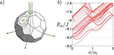
Figure 8: (Color online) a) Flux insertion on a $\mathrm{C}_{60}$ buckyball geometry. b) Many-body spectrum $E(\phi)$ on a $\mathrm{C}_{60}$ buckyball starting with $N=3$ particles and $N_{\phi}=4$ flux quanta and introducing two more flux quanta $2\times\phi_{0}$.

In Grusdt2014a, we numerically analyzed the ground state in a spherical geometry using a buckyball lattice with $N_{s}=60$ sites (see Fig. 8a). To realize a filling $\nu=1/2$ in the continuum on a sphere, the relation between particle number $N$ and flux quanta $N_{\phi}$ is $N_{\phi}=2(N-1)$. We identify the topological order of the ground state by inserting two flux quanta $\phi_{0}$ in a system with $N=3$ particles and $N_{\phi}=4$ flux quanta. The many-body spectrum $E_{\phi}$ during flux insertion is shown in Fig. 8b. We observe a single incompressible ground state with many-body gap $\Delta\simeq 0.1J$ for $U=10J$, similar to the case on a torus. Importantly, we obtain the correct counting of nearly degenerate quasi-holes states after inserting one and two flux quanta as expected from the continuum limit on a sphere. In both lattice cases we expect the ground state to be in the same topological universality class as the LN state in the continuum.

IV.3 Effective CF Lattice Model

Before we introduce the effective CF lattice model, we briefly summarize the results of the exact simulations in reference Grusdt2014a. We implemented the protocol on a $\mathrm{C}_{60}$ lattice up to $N=3$ particles. Additionally, we used a similar quasi-hole trapping potential as in eqn. (4). The numerical results show, that the state $|\Psi(t)\rangle$ prepared after three steps of the protocol is close to the LN ground state $|\mathrm{gs}\rangle$ with $N=3$ particles. Moreover, as expected from the blockade mechanism in the coherent pump, the number fluctuations $\Delta N(t)$ are small throughout the protocol.

To discuss edge effects, larger systems with many particles are required, such that bulk and edge states can be distinguished. However, using exact diagonalization only a few particles are feasible on large lattice systems with $N_{\mathrm{s}}\gtrsim 60$ sites. To simulate such a system, we need an effective model describing the low energy dynamics of the Hamiltonian (24).

In the spirit of the composite fermion principle, we assume a model of noninteracting composite fermions on a lattice. By attaching one flux quantum to a boson, as shown in Fig. 5b, an (approximately) noninteracting composite fermion is formed in a reduced magnetic field. The simplest tight-binding model with a reduced magnetic field, $\alpha^{*}=\alpha/2$, only considers nearest neighbor hopping elements $J^{*}$. Under these assumptions, the effective model is

$$\hat{\mathcal{H}}_{\mathrm{CF}}=-J^{*}\sum_{x,y}\left[\hat{c}^{\dagger}_{x+1,y}\hat{c}_{x,y}\mathrm{e}^{-i2\pi\alpha^{*}y}+\hat{c}^{\dagger}_{x,y+1}\hat{c}_{x,y}+\text{h.c.}\right],$$ (25)

where $\hat{c}^{\dagger}_{x,y}$ creates a composite fermion at site ($x,y$). The only free parameter $J^{*}$ in this model determines the time scale of the dynamics. By comparing the bandwidth of the full many-body spectrum of interacting bosons to the free CF single-particle spectrum on a $\mathrm{C}_{60}$ buckyball at $N_{\phi}=6$ flux quanta, we find $J^{*}\simeq J$.

Now, we conjecture that the effective CF lattice model describes correctly the low energy dynamics. Yet, there is no proof that the CF theory is applicable in a lattice. However, there are several hints that the essential physics can still be understood in terms of CFs. First of all, the CF picture in a lattice captures the correct counting of quasi-hole excitations . Thus, the low energy excitations should be described correctly. Moreover, the LN wavefunction is a special case of the more general CF theory, when the lowest CF-LL $n^{*}=0$ is filled. As shown in Sorensen2005 the LN wavefunction projected on a lattice describes the many-body ground state on a lattice accurately up to relatively high flux per plaquette $\alpha\simeq 0.2$. Therefore, we limit the flux per plaquette in our effective model to $\alpha^{*}\leq 0.1$. Finally, CF states from the Jain sequence Jain1989, other than the LN state, have been identified in a lattice Moeller2009; Liu2013 for small flux per plaquette. Therefore, we expect that this effective model captures the essential physics of the original many-body model in the lowest Chern band ($\mathrm{LChB}$), including the dynamics of the hole excitations. As this model is supposed to describe only the low energy regime, excitations to higher Chern bands ($\mathrm{HChB}$s) are not expected to be described correctly.

IV.4 Numerical Results

IV.4.1 Numerical implementation of the protocol

The protocol is implemented in both, the spherical geometry on a $\mathrm{C}_{60}$ buckyball as in Grusdt2014a as well as the square lattice with open boundary conditions. We use the method explained in Grusdt2014a to insert flux quanta locally.

Unlike the coherent boson pump (13), we model the coherent CF pump by coupling a CF reservoir mode to the central site of the system. The reservoir mode is refilled in each step of the protocol. Therefore, we insert at most one CF per cycle. This is similar to the blockade mechanism for bosons and therefore only justified in the limit of large interactions $U\gg J$, where corrections scale as $(\Omega/\Delta_{\text{LN}})^{2}$ (see eqn. (22)).

Moreover, we implement the quasi-hole trapping potential by including an onsite potential $g_{\mathrm{h}}$ on the central site.

As explained for the toy model, we introduce loss channels at the boundaries of the system to prevent high energy excitations. Then, we calculate the time evolution of the correlation matrix elements $\left\langle\hat{c}^{\dagger}_{x,y}\hat{c}_{x^{\prime},y^{\prime}}\right\rangle$. by solving the corresponding master equation in Lindblad form ($\hbar=1$)

$$\partial_{t}\hat{\rho}=-i[\hat{\mathcal{H}}_{\mathrm{CF}},\hat{\rho}]+\frac{1}{2}\sum_{x,y}^{\prime}2\hat{l}_{x,y}\hat{\rho}\hat{l}^{\dagger}_{x,y}-\{\hat{l}^{\dagger}_{x,y}l_{x,y},\hat{\rho}\}$$ (26)

numerically. Absorbing boundary conditions are described by the jump operators $l_{x,y}=\sqrt{\gamma_{\mathrm{Edge}}}\hat{c}_{x,y}$ with loss rate $\gamma_{\mathrm{Edge}}$ and we restrict the sum $\sum^{\prime}$ to the edge of the system.

Note, that the loss of a CF is a loss of both, a flux quantum and the boson it was attached to. Therefore, we only allow this loss term at the edge of the system, where the meaning of a free flux quantum without a particle is obsolete.

IV.4.2 Performance

To investigate the performance of the protocol, we use the spherical geometry without edges. The bandwidth $\Delta E/J$ of the $\mathrm{C}_{60}$ buckyball with up to $N_{\phi}=6$ flux quanta is small and thus we can neglect the effect of dispersive bands. In section III.4, we have seen that the topological pump as well as the coherent pump in the continuum need sufficiently long times $T_{\phi},T_{\Omega}\gg\Delta_{\text{LN}}^{-1}$ to avoid nonadiabatic excitations. The excitation probability to the excitonic states scale as $P_{\phi}\sim T_{\phi}^{-2},P_{\Omega}\sim T_{\Omega}^{-2}\sim\Omega^{2}$ (see eqns. (21), (22)). Here, we show that the scaling for $P_{\phi},P_{\Omega}$ also holds for the lattice in the perturbative regime.

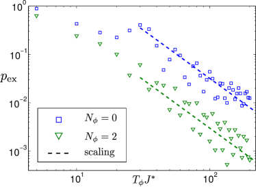
Figure 9: (Color online) Shown is the excitation probability $p_{\mathrm{ex}}$ to high energy states in the case of flux insertion. Starting with particle number $N=1$ ($N=3$) in the ground state $|\mathrm{gs}\rangle$ at $N_{\phi}=0$ ($N_{\phi}=2$) flux quanta, we insert one flux quantum and analyze the probability $p_{\mathrm{ex}}$ of being in an excited state for various flux insertion times $T_{\phi}$. The dashed lines indicate the expected scaling from eqn. (21) in section III.4.

Firstly, we analyze the excitation probability $p_{\mathrm{ex}}$ in the case of flux insertion. We start from the ground state $|\mathrm{gs}\rangle$ with $N=1$ ($N=3$) particle(s) at $N_{\phi}=0$ ($N_{\phi}=2$) flux quanta and insert one flux quantum in time $T_{\phi}$ to create a CF quasi-hole excitation $|\text{qh}\rangle$. Figure 9 shows the probability $p_{\mathrm{ex}}$ for excitation of higher bands. Besides an oscillatory behavior with increasing duration $T_{\phi}$, we confirm the expected scaling $P_{\phi}\sim T_{\phi}^{-2}$in the perturbative regime.

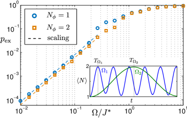
Figure 10: (Color online) We show the excitation probability $p_{\mathrm{ex}}$ to high energy states for different Rabi-frequencies $\Omega$ in the coherent CF pump. Starting from the quasi-hole state with $N_{\phi}=1$ ($N_{\phi}=2$) flux quantum, we coherently couple to the ground state with $N=2$ ($N=3$) particles for various Rabi-frequencies $\Omega$. The dashed lines indicate the expected scaling from section III.4. In the inset, we extract the $\pi$-pulse time $T_{\Omega}$ when the maximal number of particles is in the system, for two different values of $\Omega$.

To analyze the excitation probability $p_{\mathrm{ex}}$ for the coherent CF pump, we start from the quasi-hole state $|\text{qh}\rangle$ at $N_{\phi}=1$ ($N_{\phi}=2$) flux quantum. The coherent pump is coupled resonantly to the hole excitation for different bare Rabi-frequencies $\Omega$. In Fig. 10 we plot $p_{\mathrm{ex}}$ for different $\Omega$. The time $T_{\Omega}$ needed for a $\pi$-pulse is determined by the maximal achievable particle number $\left\langle N\right\rangle$ (see inset Fig. 10). For time $T_{\Omega}$, we extract the excitation probability $p_{\mathrm{ex}}$ of being not in the ground state with $N=2$ ($N=3$) particles. We find excellent agreement with the expected scaling in the perturbative regime.

IV.4.3 Dispersive bands – quasi-hole trapping

As noted in the toy model section II, the finite bandwidth leads to an intrinsic dispersion of the quasi-hole excitations. Without trapping the hole excitations, the coherent pump cannot replenish them efficiently.

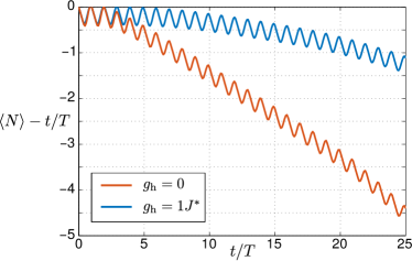
Figure 11: (Color online) Shown is the number of particles $\left\langle N\right\rangle$ during the protocol in time $t/T$ in a system with and without trapping potential $g_{\mathrm{h}}$. The lattice size is $11\times 11$ with an effective flux per plaquette $\alpha^{*}=0.1$. We insert flux in time $T_{\phi}=60/J^{*}$. The $\pi$-pulse time $T_{\Omega}$ for $g_{\mathrm{h}}=0$ ($g_{\mathrm{h}}=1J^{*}$) is $T_{\Omega}=100/J^{*}$ ($T_{\Omega}=130/J^{*}$).

We numerically analyze the effect of dispersive bands on a square lattice. The results are shown in Fig. 11, where we compare the number of CFs $\left\langle N\right\rangle(t)$ for 25 cycles of the protocol with and without quasi-hole trapping potential $g_{\mathrm{h}}$. Here, $T=T_{\phi}+T_{\Omega}$ is the time needed for one step of the protocol. The trapping potential improves the efficiency of the growing scheme already after three steps. Therefore, we include the quasi-hole trapping potential $g_{\mathrm{h}}$ for the following discussions.

IV.4.4 Finite systems – edge decay

Let us finally discuss the effects of a finite system, where edge states are present. As explained in the toy model section II, during the protocol edge states will transport particles to high energy states. To reach a homogeneous particle density in the bulk of the $\mathrm{LChB}$, absorbing boundaries can be implemented to prevent excitations to $\mathrm{HChB}$s.

In the case of open boundary conditions, we identify three different regimes in the single particle spectrum of the CFs, shown in Fig. 12a. Due to the finite size of the system, edge states occur between the states of the $\mathrm{LChB}$ and those of the $\mathrm{HChB}$. Crucially, the effective CF model on the lattice is not supposed to describe the dynamics of the high energy states correctly. To prepare a LN type state in the bulk of a finite systems, it is necessary to avoid high energy excitations.

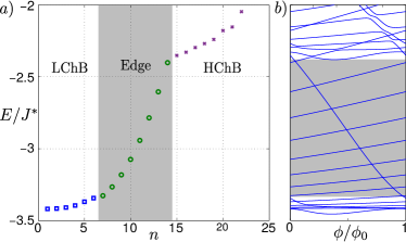
Figure 12: (Color online) a) Low energy spectrum of the CF Hamiltonian (25) with $\alpha^{*}=0.1$ and lattice size $11\times 11$. States are labeled with number $n$. We identify three different sectors using additionally the density distribution of the states: Lowest Chern band ($\mathrm{LChB}$) $n=1,\ldots,6$, edge states ($\mathrm{Edge}$) $n=7,\ldots,14$ and higher Chern bands ($\mathrm{HChB}$s) $n\geq 15$. b) Energy spectrum during insertion of one flux quantum $\phi_{0}$ with parameters as in a).

The free CF energy spectrum of a finite system with trapping potential $g_{\mathrm{h}}$ during adiabatic flux insertion is depicted in Fig. 12b. Besides the creation of a hole excitation in the $\mathrm{LChB}$, edge states occur connecting the low and high energy states. Due to the edge states, particles will be excited to the $\mathrm{HChB}$s of the system during the protocol.

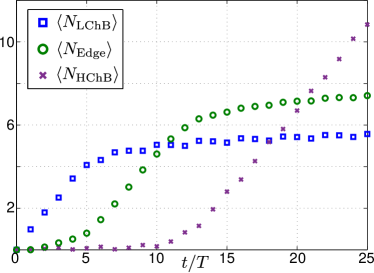
Figure 13: (Color online) Particle number $\left\langle N_{\mathrm{LChB}}\right\rangle$, $\left\langle N_{\mathrm{Edge}}\right\rangle$, $\left\langle N_{\mathrm{HChB}}\right\rangle$ in the three different energy sectors, defined in Fig. 12a, after each cycle in the protocol. The parameters used here are the same as in Fig. 11 with trapping potential $g_{\mathrm{h}}$.

This is shown in Fig. 13, where we analyze the particle number $\left\langle N_{\mathrm{LChB}}\right\rangle,\left\langle N_{\mathrm{Edge}}\right\rangle,\left\langle N_{\mathrm{HChB}}\right\rangle$ in the three different regions, defined in Fig. 12a, after each step of the protocol. As expected, in the first few steps the number of particles in the $\mathrm{LChB}$ $\left\langle N_{\mathrm{LChB}}\right\rangle$ increases. However, before the $\mathrm{LChB}$ is completely filled, edge states are populated and as a consequence the number of states in $\mathrm{HChB}$s $\left\langle N_{\mathrm{HChB}}\right\rangle$ starts to increase. Figure 14a shows the population $p_{n}$ of the first CF states (labeled with integer $n$) after 25 steps of the protocol.

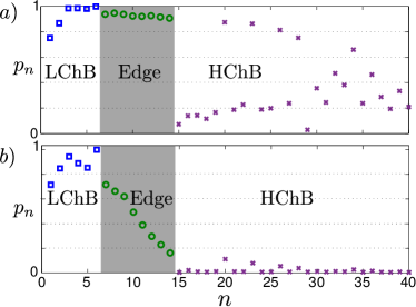
Figure 14: (Color online) Population $p_{n}$ of the low energy CF states at the end of the protocol. a) Parameters as in Fig. 11 after 25 steps of the protocol and b) after 35 steps of the protocol with absorbing boundary conditions ($\gamma_{\mathrm{Edge}}=0.0025J^{*}$).

To avoid the population of $\mathrm{HChB}$s, we include absorbing boundaries as discussed in the toy model. Since edge states are localized at the boundaries of the system, the bulk properties of the system will only slightly be affected. However, for a properly chosen decay rate $\gamma_{\mathrm{Edge}}$ on the boundary, edge excitations will be lost before they reach the $\mathrm{HChB}$ during the protocol. In Fig. 14b we show the population of the first CF states after 35 steps of the protocol. The $\mathrm{HChB}$s are only very weakly populated due to the absorbing boundary conditions. The CF density $\rho^{*}$ of the last cycle is shown in Fig. 1. In terms of the CFs we reach an average CF filling factor of $\nu^{*}\simeq 0.9$ of the $\mathrm{LChB}$, which is close to the optimal value $\nu^{*}=1$.

V Summary & Outlook

In conclusion, we discussed a protocol which allows to grow topologically ordered states in interacting many-body systems. We explained all necessary ingredients using the SLBHM as a simple toy model. We showed that in the flat-band limit a combination of a topologically protected Thouless pump Thouless1982, creating a local hole excitation, and a coherent pump, refilling the hole excitation, are sufficient. Moreover, we extended the protocol to the case of dispersive bands and finite systems with edges.

Furthermore, we discussed the protocol in detail in both, the continuum case and the lattice case of fractional quantum Hall systems. In the continuum, we estimated the fidelity of the protocol depending on the particle number $N$. To describe numerically large lattice systems with many particles, we introduced an effective model based on the CF description of the FQHE. This allows us to simulate large systems and include edge effects. We showed, that a quasi-hole trapping potential can be used in the case of dispersive bands to maintain a high efficiency of the protocol. Moreover, absorbing boundaries are used in finite systems, where edge states would transport excitations to higher bands. We showed that in the case of dispersive bands and even in the presence of edge states, a high CF filling factor $\nu^{*}\simeq 0.9$ is achievable, in large systems with more than 10 particles.

We believe, that our protocol can be used to grow other exotic states than the LN state, e.g. the Moore-Read Pfaffian Moore1991. So far, we did not consider experimental realizations. However, ultracold gases as well as photonic systems are promising candidates. Moreover, the efficiency of our scheme can be increased by introducing multiple pairs of topological and coherent pumps.

Appendix A Flux Insertion in the IQHE

To address the problem of flux insertion, we briefly review the Landau Level (LL) problem. To this end, we use a basis, which is not typically used in standard textbooks. It will turn out, that this basis allows a simple understanding of the flux insertion process.

A.1 Landau Level

The LL Hamiltonian in symmetric gauge, $\bm{A}=B/2(-y,x,0)$, is ($\hbar=1$)

$$\hat{\mathcal{H}}_{0} =\frac{1}{2M}\left(\bm{p}-\bm{A}\right)^{2}$$ (27)

$$=\frac{1}{2M}\bm{p}^{2}+\frac{1}{2}M\left(\frac{\omega_{c}}{2}\right)^{2}\left(x^{2}+y^{2}\right)-\frac{\omega_{c}}{2}L_{z}.$$

As angular momentum $L_{z}$ is a conserved quantity, i.e. $[\hat{\mathcal{H}}_{0},L_{z}]=0$ , we can use the eigenbasis $|n_{r},\ell_{r}\rangle$ of a two dimensional harmonic oscillator. Here, $n_{r}=0,1,\ldots$ corresponds to the energy levels of the harmonic oscillator and $\ell_{r}\in\mathbb{Z}$ to those of the angular momentum. We obtain

$$L_{z}|n_{r},\ell_{r}\rangle =\ell_{r}|n_{r},\ell_{r}\rangle$$ (28)

$$\hat{\mathcal{H}}_{0}|n_{r},\ell_{r}\rangle =\frac{\omega_{c}}{2}\left(2n_{r}+|\ell_{r}|-\ell_{r}\right)|n_{r},\ell_{r}\rangle.$$ (29)

The energy spectrum of both, the harmonic oscillator and the LL, are shown in Fig. 15.

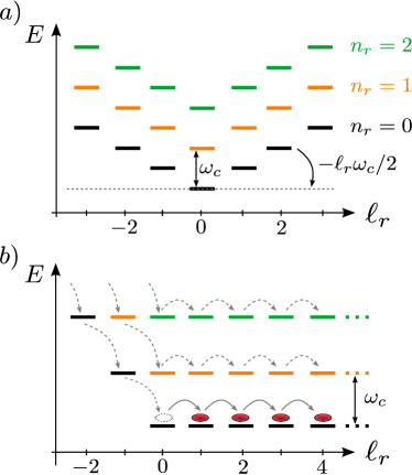
Figure 15: (Color online) a) Schematic picture of the Landau Level construction using the two dimensional harmonic oscillator basis $|n_{r},\ell_{r}\rangle$. b) In the flux insertion process, the angular momentum $\ell_{r}$ is increased by one, while keeping the quantum number $n_{r}$ fixed.

A.2 Flux insertion

In 1981 Laughlin Laughlin1981 explained the quantization of the Hall current using the argument of flux insertion. This idea can be used to create localized hole excitations in the quantum Hall effect. The idea is as follows. After introducing one flux quantum $\phi_{0}$ adiabatically in the center, a circular electric field is generated. The Hall response thus leads to a radial outwards current creating a hole in the center of the system. As shown below, the quasi-hole excitation is quantized.

To realize Laughlin’s argument, we include in eqn. (27) the vectorpotential

$$\bm{A}_{\phi}=-\frac{\phi(t)}{2\pi r}\bm{e}_{\varphi}.$$ (30)

Defining a new angular momentum

$$L_{z}^{{}^{\prime}}=L_{z}+\phi/\phi_{0},$$ (31)

we obtain the same structure as in eqn. (27). However, by adiabatically increasing $\phi(t)$, we change the angular momentum of the system. By inserting one flux quantum $\phi_{0}$, we increase the angular momentum $\ell_{r}$ of all states by one, while the quantum number $n_{r}$ stays fixed. This generates the spectral flow depicted in FIG. 15b.

Appendix B Nonadiabatic Corrections in the Flux Insertion Process

To calculate the probability $P_{\phi}$ of exciting particles to higher LLs during flux insertion in the noninteracting case, we use the basis discussed in appendix A. By inserting adiabatically one flux quantum $\phi(t)=\phi_{0}\ t/T_{\phi}$ in time $T_{\phi}\gg 1/\omega_{c}$, the angular momentum $\ell_{r}(t)$ increases by one, i.e. $\ell_{r}(T_{\phi})=\ell_{r}(0)+1$. Therefore, starting from state $|n_{r},\ell_{r}(0)\rangle$, we end in the state $|n_{r},\ell_{r}(0)+1\rangle$. Here, we calculate perturbatively in the regime $(\omega_{c}T_{\phi})^{-1}\ll 1$ the scaling of the probability $P_{\phi}$ of exciting particles to higher LLs.

The nonadiabatic coupling $g_{\phi}$ between different LLs $n_{r}\neq n_{r}^{\prime}$ is

$$g_{\phi} =\langle n_{r}^{\prime},\ell_{r}|-i\partial_{t}|n_{r},\ell_{r}\rangle$$

$$=\langle n_{r}^{\prime},\ell_{r}|-i\partial_{\ell_{r}}|n_{r},\ell_{r}\rangle/T_{\phi}=\kappa/T_{\phi}.$$ (32)

In Fig. 16, we plot the coupling $|\kappa|$ from the lowest LL $n_{r}^{\prime}=0$ to higher LLs $n_{r}$ for different angular momentum $\ell_{r}$. As expected, the coupling to higher LLs decreases.

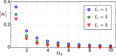
Figure 16: (Color online) Coupling $|\kappa|$ from the lowest LL $n_{r}^{\prime}=0$ to higher LLs $n_{r}$ for different angular momentum $\ell_{r}$.

To estimate the scaling of $P_{\phi}$ with flux insertion time $T_{\phi}$ in the perturbative regime $(\omega_{c}T_{\phi})^{-1}\ll 1$, we consider a simple two level approximation with LLs $n_{r},n_{r}+1$ and constant coupling $\kappa$. Starting from the state $|n_{r},\ell_{r}\rangle$, we calculate in first order perturbation theory the probability for ending in state $|n_{r}+1,\ell_{r}\rangle$. We obtain approximately

$$P_{\phi}\simeq\frac{\kappa^{2}}{(\omega_{c}T_{\phi})^{2}}2\left(1-\cos(\omega_{c}T_{\phi})\right).$$ (33)

We expect, that the scaling of $P_{\phi}$ with $T_{\phi}$ in the interacting case to be the same as in the noninteracting case, when the cyclotron frequency $\omega_{c}$ is replaced by the many-body gap $\Delta_{\text{LN}}$. This leads to eqn. (21).

Appendix C Nonadiabatic Corrections in the Coherent Pump Process

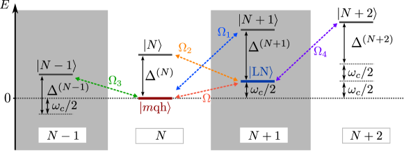
Figure 17: (Color online) Schematic overview over the coupling between states in different particle sectors in first order in $\Omega/\Delta_{\text{LN}}$. Starting from the quasi-hole state $|\text{qh}\rangle$ of $N$ particles or the LN state $|\text{LN}\rangle$ with $N+1$ particles, the particle sectors from $N-1$ to $N+2$ are involved. $\Omega_{i}$ denote the many-body Rabi-frequencies reduced by their Franck-Condon factors with respect to the bare Rabi-frequency $\Omega$. The many-body gaps $\Delta^{(N)}\geq\Delta_{\text{LN}}$ to the excitonic states $|N\rangle$ are multiples of the LN gap $\Delta_{\text{LN}}$.

In zeroth order in $\Omega/\Delta_{\text{LN}}\ll 1$, the coherent pump couples the quasi-hole state $|\text{qh}\rangle$ with $N$ particles to the LN state with $N+1$ particles. The Rabi-frequency is $\Omega$ and we choose a driving frequency $\omega_{c}/2$, resonant with the zero-interaction energy LN state $|\text{LN}\rangle$. Thereby, in the continuum no total angular momentum $\Delta L_{z}$ is transferred.

In first order, we couple the quasi-hole state $|\text{qh}\rangle$ and the LN state $|\text{LN}\rangle$ to the excitonic states in different particle sectors from $N-1$ to $N+2$, as illustrated schematically in Fig. 17. For simplicity, only one excitonic state $|N\rangle$ in each particle sector with many-body gap $\Delta^{(N)}$ is shown. The effective Rabi-frequencies $\Omega_{i}$, reduced by many-body Franck-Condon factors, are labeled by an index $i=1,\ldots,4$.

For the model discussed in section III, we find, that the Franck-Condon factors

$$\Omega_{2}/\Omega =\langle N|\hat{b}_{0,0}|\text{LN}\rangle=0$$ (34)

$$\Omega_{3}/\Omega =\langle N-1|\hat{b}_{0,0}|\text{qh}\rangle=0$$ (35)

vanish. Furthermore, we calculate perturbatively the excitation probability $P_{\Omega}$ of excitonic states in first order in $\Omega/\Delta_{\text{LN}}\ll 1$. Starting from the quasi-hole state $|\text{qh}\rangle$, after a $\pi$-pulse of duration $T_{\Omega}=\pi/2\Omega$, we obtain approximately the result in eqn. (21). There, the factor $\sigma_{N}$ is defined as

$$\sigma_{N}^{2}=\left(\frac{\pi}{2}\right)^{2}\sum_{j}\frac{\Omega_{1j}^{2}/\Omega^{2}}{\Delta_{j}^{(N+1)2}/\Delta_{\text{LN}}^{2}}+\frac{\Omega_{4j}^{2}/\Omega^{2}}{\Delta_{j}^{(N+2)2}/\Delta_{\text{LN}}^{2}},$$ (36)

where the sum over $j$ includes all states in each of the particle sectors with gap $\Delta_{j}^{(N)}\geq\Delta_{\text{LN}}$. For different particle numbers $N$, we calculated the prefactor $\sigma_{N}$ in Fig. 7.