Thick brane models in generalized theories of gravity

D. Bazeia1, A. S. Lobão Jr.2 and R. Menezes3,4 1Departamento de Física, Universidade Federal da Paraíba, 58051-970 João Pessoa, PB, Brazil
2Escola Técnica de Saúde de Cajazeiras, Universidade Federal de Campina Grande, 58900-000 Cajazeiras, PB, Brazil
3Departamento de Ciências Exatas, Universidade Federal da Paraíba, 58297-000 Rio Tinto, PB, Brazil and
4Departamento de Física, Universidade Federal de Campina Grande, 58109-970 Campina Grande, PB, Brazil.
Abstract

This work deals with thick braneworld models, in an environment where the Ricci scalar is changed to accommodate the addition of two extra terms, one depending on the Ricci scalar itself, and the other, which takes into account the trace of the energy-momentum tensor of the scalar field that sources the braneworld scenario. We suppose that the scalar field engenders standard kinematics, and we show explicitly that the gravity sector of this new braneworld scenario is linearly stable. We illustrate the general results investigating two distinct models, focusing on how the brane profile is changed in the modified theories.

pacs:
11.27.+d, 11.10.Kk

I introduction

This work deals with braneworld models in the presence of scalar fields RS ; GW ; F in an AdS5 geometry with a single extra dimension of infinite extent. Differently from the original Randall and Sundrum (RS) proposal presented in RS , which leads to the thin braneworld scenario, the coupling with scalar fields is also of interest and leads to another, thick braneworld scenario GW ; F ; C . The presence of a scalar field makes the warp function to behave smoothly, leading to a thick braneworld scenario. This possibility has opened a new area of study, and here we quote Ref. G for some works on the subject.

In the current work, we go beyond General Relativity. Before doing this, however, we should care about issues concerning the presence of degrees of freedom which may lead to instabilities in these theories, and here we recommend the interesting reviews on the subject ghost . To go beyond General Relativity, we add two distinct contributions, one taking the metric tensor gμνsubscript𝑔𝜇𝜈g_{\mu\nu} to change R=gμνRμν𝑅subscript𝑔𝜇𝜈superscript𝑅𝜇𝜈R=g_{\mu\nu}R^{\mu\nu} (the Ricci scalar, the trace of the Ricci tensor) to F(R)𝐹𝑅F(R), and the other, modifying Einstein’s equation with the inclusion of auxiliary fields, as suggested recently in Ref. psv . To be more specific, we recall that the modification that changes R𝑅R into F(R)𝐹𝑅F(R) in the Einstein-Hilbert action is older and was reviewed in Ref. FR . The modification introduced in the presence of auxiliary fields is more recent psv and was studied in Refs. c1 ; c2 within the cosmological context, to see how the auxiliary fields may contribute to the cosmic evolution. Moreover, it has also been recently studied within the thick braneworld context, in five dimensions with a single extra dimension of infinite extent gly ; we . See also Refs. m1 ; m2 for other related studies on thick branes.

In order to widen the interest in the work, here we add together both R𝑅R and T=gμνTμν𝑇subscript𝑔𝜇𝜈superscript𝑇𝜇𝜈T=g_{\mu\nu}T^{\mu\nu} (the trace of the energy-momentum tensor) into F(R,T)𝐹𝑅𝑇F(R,T) to describe the generalized model, inspired by the recent investigations RT1 ; RT2 . We then study how the two modifications act to change the standard braneworld scenario, in an AdS5𝐴𝑑subscript𝑆5AdS_{5} braneworld geometry with a single extra spatial dimension of infinite extent. We implement the investigation in Sec. II, where we discuss the general theory, including linear stability of the gravity sector. We then study two specific new models in Sec. III, working out the most important results of the models. As one knows, scalar fields play a fundamental role in cosmology as possible explanations for inflation, late time acceleration, and dark matter, among other issues. Also, scalar fields are fundamental sources in the thick braneworld scenario with a single extra dimension of infinite extent. Thus, here we investigate scenarios described by a single real scalar field to source the thick brane configuration, leaving aside studies related to cosmology. We then end the work in Sec. IV, where we include our comments and conclusions.

II The problem

We start investigating a model that describes generalized gravity coupled to a scalar field in five-dimensional space-time, with a single extra dimension y𝑦y of infinite extent. The model is controlled by an action of the form

S=d4x𝑑y|g|(14F(R,T)+s),𝑆superscript𝑑4𝑥differential-d𝑦𝑔14𝐹𝑅𝑇subscript𝑠S=\int d^{4}x\,dy\sqrt{|g|}\Big{(}-\frac{1}{4}F(R,T)+{\cal L}_{s}\Big{)}\,, (1)

where R𝑅R and T𝑇T represents the Ricci scalar and the trace of the energy-momentum tensor, and ssubscript𝑠{\cal L}_{s} describes the source Lagrange density, which we suppose is of the form

s=12aϕaϕV(ϕ).subscript𝑠12subscript𝑎italic-ϕsuperscript𝑎italic-ϕ𝑉italic-ϕ{\cal L}_{s}=\frac{1}{2}\nabla_{a}\phi\nabla^{a}\phi-V(\phi)\,. (2)

It engenders standard kinematics, and we are using 4πG(5)=14𝜋superscript𝐺514\pi G^{(5)}=1, g=det(gab)𝑔𝑑𝑒𝑡subscript𝑔𝑎𝑏g=det(g_{ab}), a,b=0,1,,4formulae-sequence𝑎𝑏014a,b=0,1,...,4 and the signature of the metric is (+)(+----). We focus attention on the profile of the thick braneworld scenario, so the addition of fermions and gauge fields will not be considered in this work. We take the spacetime coordinates and fields as dimensionless quantities, and we use Greek indices for the embedded (3+1)-dimensional space, μ,ν=0,1,2,3formulae-sequence𝜇𝜈0123\mu,\nu=0,1,2,3.

We can use the source Lagrange density (2) to write the energy-momentum tensor in the form

Tab=12gabcϕcϕ+gabV+aϕbϕ,subscript𝑇𝑎𝑏12subscript𝑔𝑎𝑏subscript𝑐italic-ϕsuperscript𝑐italic-ϕsubscript𝑔𝑎𝑏𝑉subscript𝑎italic-ϕsubscript𝑏italic-ϕT_{ab}=-\frac{1}{2}g_{ab}\nabla_{c}\phi\nabla^{c}\phi+g_{ab}V+\nabla_{a}\phi\nabla_{b}\phi\,, (3)

which contributes to give the trace

T=(3/2)aϕaϕ+5V.𝑇32subscript𝑎italic-ϕsuperscript𝑎italic-ϕ5𝑉T=-(3/2)\nabla_{a}\phi\nabla^{a}\phi+5V. (4)

Moreover, the equation of motion for the scalar field has the form

aaϕ+34a(FTaϕ)+54VϕFT+Vϕ=0,subscript𝑎superscript𝑎italic-ϕ34subscript𝑎subscript𝐹𝑇superscript𝑎italic-ϕ54subscript𝑉italic-ϕsubscript𝐹𝑇subscript𝑉italic-ϕ0\displaystyle\nabla_{a}\nabla^{a}\phi+\frac{3}{4}\nabla_{a}\Big{(}F_{T}\nabla^{a}\phi\Big{)}+\frac{5}{4}V_{\phi}F_{T}+V_{\phi}=0, (5)

where Vϕ=dV/dϕsubscript𝑉italic-ϕ𝑑𝑉𝑑italic-ϕV_{\phi}=dV/d\phi, and FR=dF/dRsubscript𝐹𝑅𝑑𝐹𝑑𝑅F_{R}=dF/dR, FT=dF/dTsubscript𝐹𝑇𝑑𝐹𝑑𝑇F_{T}=dF/dT, etc. By varying the action of the gravitational field with respect to the metric tensor we obtain the modified Einstein equation

FRRab12gabF+(gabab)FRsubscript𝐹𝑅subscript𝑅𝑎𝑏12subscript𝑔𝑎𝑏𝐹subscript𝑔𝑎𝑏subscript𝑎subscript𝑏subscript𝐹𝑅\displaystyle F_{R}R_{ab}-\frac{1}{2}g_{ab}F+\Big{(}g_{ab}\Box-\nabla_{a}\nabla_{b}\Big{)}F_{R}
=2Tab+32FTaϕbϕ.absent2subscript𝑇𝑎𝑏32subscript𝐹𝑇subscript𝑎italic-ϕsubscript𝑏italic-ϕ\displaystyle=2T_{ab}+\frac{3}{2}F_{T}\nabla_{a}\phi\nabla_{b}\phi\,. (6)

We study the case of a flat brane, with the line element

ds2=e2Aημνdxμdxνdy2,𝑑superscript𝑠2superscript𝑒2𝐴subscript𝜂𝜇𝜈𝑑superscript𝑥𝜇𝑑superscript𝑥𝜈𝑑superscript𝑦2ds^{2}=e^{2A}\eta_{\mu\nu}dx^{\mu}dx^{\nu}-dy^{2}\,, (7)

where A𝐴A is the warp function, e2Asuperscript𝑒2𝐴e^{2A} is the warp factor and ημνsubscript𝜂𝜇𝜈\eta_{\mu\nu} is the 4-dimensional Minkowski metric, with signature (+,,,)(+,-,-,-). We consider the case where both A𝐴A and ϕitalic-ϕ\phi are static and only depends on the extra dimension, that is, A=A(y)𝐴𝐴𝑦A=A(y) and ϕ=ϕ(y)italic-ϕitalic-ϕ𝑦\phi=\phi(y). We then get

(1+34FT)ϕ′′+[(4+3FT)A+34FT]ϕ=(1+54FT)Vϕ,134subscript𝐹𝑇superscriptitalic-ϕ′′delimited-[]43subscript𝐹𝑇superscript𝐴34superscriptsubscript𝐹𝑇superscriptitalic-ϕ154subscript𝐹𝑇subscript𝑉italic-ϕ\Big{(}1+\frac{3}{4}F_{T}\Big{)}\phi^{\prime\prime}+\Big{[}(4+3F_{T})A^{\prime}+\frac{3}{4}F_{T}^{\prime}\Big{]}\phi^{\prime}=\Big{(}1+\frac{5}{4}F_{T}\Big{)}V_{\phi}\,, (8)

where the prime denotes derivative with respect to the extra dimension. Also, the modified Einstein equation becomes

23ϕ2(1+34FT)23superscriptitalic-ϕ2134subscript𝐹𝑇\displaystyle\frac{2}{3}\phi^{\prime 2}\Big{(}\!1\!+\!\frac{3}{4}F_{T}\!\Big{)}\!\!\! =\displaystyle= A′′FR+13AFR13FR′′,superscript𝐴′′subscript𝐹𝑅13superscript𝐴superscriptsubscript𝐹𝑅13superscriptsubscript𝐹𝑅′′\displaystyle\!\!\!-A^{\prime\prime}F_{R}+\frac{1}{3}A^{\prime}F_{R}^{\prime}-\frac{1}{3}F_{R}^{\prime\prime}\,, (9a)
V(ϕ)ϕ22(1+32FT)𝑉italic-ϕsuperscriptitalic-ϕ22132subscript𝐹𝑇\displaystyle\!\!\!\!\!\!V(\phi)\!-\!\frac{\phi^{\prime 2}}{2}\Big{(}\!1\!+\!\frac{3}{2}F_{T}\!\Big{)}\!\!\! =\displaystyle= 2(A2+A′′)FRF42AFR.2superscript𝐴2superscript𝐴′′subscript𝐹𝑅𝐹42superscript𝐴superscriptsubscript𝐹𝑅\displaystyle\!\!\!2(A^{\prime 2}\!\!+\!A^{\prime\prime})F_{R}\!-\!\frac{F}{4}\!-\!2A^{\prime}F_{R}^{\prime}. (9b)

As it is standard check, here we also note that the set of equations (9) leads us with the equation of motion (8).

An important characteristic of the brane is its tension, which is given by

𝒯=𝑑yρ(y),𝒯differential-d𝑦𝜌𝑦{\cal T}=\int dy\,\rho(y)\,, (10)

where ρ(y)=e2As𝜌𝑦superscript𝑒2𝐴subscript𝑠\rho(y)=-e^{2A}{\cal L}_{s} is the energy density of the brane.

The next important step is to check if the modification proposed above contribute to destabilize the geometric degrees of freedom of the braneworld model. We investigate this issue studying linear stability of the gravity sector in the usual way.

II.1 Stability

The investigation of linear stability of the braneworld model can be done assuming that the metric is perturbed in the form

ds2=e2A(y)[ημν+hμν(y,x)]dxμdxνdy2.𝑑superscript𝑠2superscript𝑒2𝐴𝑦delimited-[]subscript𝜂𝜇𝜈subscript𝜇𝜈𝑦𝑥𝑑superscript𝑥𝜇𝑑superscript𝑥𝜈𝑑superscript𝑦2ds^{2}=e^{2A(y)}\Big{[}\eta_{\mu\nu}+h_{\mu\nu}(y,x)\Big{]}dx^{\mu}dx^{\nu}-dy^{2}\,. (11)

Furthermore, the scalar field is written in the form

ϕ=ϕ(y)+ξ(y,x).italic-ϕitalic-ϕ𝑦𝜉𝑦𝑥\phi=\phi(y)+\xi(y,x)\,. (12)

The first-order contributions in hh and ξ𝜉\xi that follow from the equations of motion lead us to

[12hμν′′+2Ahμν+12ημνAh12e2A(4)hμν+\displaystyle\Big{[}\frac{1}{2}h_{\mu\nu}^{\prime\prime}+2A^{\prime}h_{\mu\nu}^{\prime}+\frac{1}{2}\eta_{\mu\nu}A^{\prime}h^{\prime}-\frac{1}{2}e^{-2A}\Box^{(4)}h_{\mu\nu}+
+12e2A(μαhαν+ναhαμμνh)]FR\displaystyle+\frac{1}{2}e^{-2A}\Big{(}\partial_{\mu}\partial^{\alpha}h_{\alpha\nu}+\partial_{\nu}\partial^{\alpha}h_{\alpha\mu}-\partial_{\mu}\partial_{\nu}h\Big{)}\Big{]}F_{R}-
e2AμνP(x,y)+12hμνFR=Q(x,y)ημν,superscript𝑒2𝐴subscript𝜇subscript𝜈𝑃𝑥𝑦12superscriptsubscript𝜇𝜈superscriptsubscript𝐹𝑅𝑄𝑥𝑦subscript𝜂𝜇𝜈\displaystyle-e^{-2A}\partial_{\mu}\partial_{\nu}P(x,y)+\frac{1}{2}h_{\mu\nu}^{\prime}F_{R}^{\prime}=Q(x,y)\eta_{\mu\nu}\,, (13)

where h=hμμh=h^{\mu}{}_{\mu}. For simplicity, we have introduced the functions P(x,y)𝑃𝑥𝑦P(x,y) and Q(x,y)𝑄𝑥𝑦Q(x,y), which are defined as

P(x,y)𝑃𝑥𝑦\displaystyle P(x,y)\!\! =\displaystyle= [h′′+5Ah+e2A(μνhμν(4)h)]FRRdelimited-[]superscript′′5superscript𝐴superscriptsuperscript𝑒2𝐴superscript𝜇superscript𝜈subscript𝜇𝜈superscript4subscript𝐹𝑅𝑅\displaystyle\!\!\Big{[}h^{\prime\prime}+5A^{\prime}h^{\prime}+e^{-2A}\Big{(}\partial^{\mu}\partial^{\nu}h_{\mu\nu}-\Box^{(4)}h\Big{)}\Big{]}F_{RR} (14)
+[5Vϕξ+3ϕξ+(ϕ2+2V)h]FRT,delimited-[]5subscript𝑉italic-ϕ𝜉3superscriptitalic-ϕsuperscript𝜉superscriptitalic-ϕ22𝑉subscript𝐹𝑅𝑇\displaystyle\!\!+\Big{[}5V_{\phi}\xi+3\phi^{\prime}\xi^{\prime}+(\phi^{\prime 2}+2V)h\Big{]}F_{RT}\,,

and

Q(x,y)𝑄𝑥𝑦\displaystyle Q(x,y)\!\! =\displaystyle= 3AP(x,y)+P′′(x,y)e2A(4)P(x,y)+3superscript𝐴superscript𝑃𝑥𝑦superscript𝑃′′𝑥𝑦limit-fromsuperscript𝑒2𝐴superscript4𝑃𝑥𝑦\displaystyle\!\!3A^{\prime}P^{\prime}(x,y)+P^{\prime\prime}(x,y)-e^{-2A}\Box^{(4)}P(x,y)+ (15)
+(Ah+12h)FR+2Vϕξ+2ϕξ+[12FT\displaystyle\!\!+\Big{(}A^{\prime}h+\frac{1}{2}h^{\prime}\Big{)}F_{R}^{\prime}+2V_{\phi}\xi+2\phi^{\prime}\xi^{\prime}+\Big{[}\frac{1}{2}F_{T}-
FRT(4A2+A′′)][5Vϕξ+3ϕξ+(ϕ2+2V)h]\displaystyle\!\!-F_{RT}(4A^{\prime 2}\!+\!A^{\prime\prime})\!\Big{]}\!\Big{[}5V_{\phi}\xi\!+\!3\phi^{\prime}\xi^{\prime}\!\!+\!(\phi^{\prime 2}\!\!+\!2V)h\Big{]}\!\!-
[(4A2+A′′)FRR12FR][h′′+5Ah+\displaystyle\!\!-\Big{[}(4A^{\prime 2}+A^{\prime\prime})F_{RR}-\frac{1}{2}F_{R}\Big{]}\Big{[}h^{\prime\prime}+5A^{\prime}h^{\prime}+
+e2A(μνhμν(4)h)].\displaystyle\!\!+e^{-2A}\Big{(}\partial^{\mu}\partial^{\nu}h_{\mu\nu}-\Box^{(4)}h\Big{)}\Big{]}\,.

If we take F(R,T)R𝐹𝑅𝑇𝑅F(R,T)\to R, in the case of General Relativity we get P(x,y)=0𝑃𝑥𝑦0P(x,y)=0 and

Q(x,y)𝑄𝑥𝑦\displaystyle Q(x,y) =\displaystyle= 2Vϕξ+2ϕξ+12h′′+52Ah2subscript𝑉italic-ϕ𝜉2superscriptitalic-ϕsuperscript𝜉12superscript′′52superscript𝐴superscript\displaystyle 2V_{\phi}\xi+2\phi^{\prime}\xi^{\prime}+\frac{1}{2}h^{\prime\prime}+\frac{5}{2}A^{\prime}h^{\prime} (16)
+12e2A(μνhμν(4)h).12superscript𝑒2𝐴superscript𝜇superscript𝜈subscript𝜇𝜈superscript4\displaystyle+\frac{1}{2}e^{-2A}\Big{(}\partial^{\mu}\partial^{\nu}h_{\mu\nu}-\Box^{(4)}h\Big{)}.

We can simplify the investigation of stability considering the transverse traceless components of metric fluctuations, that is, we take

μhμν=0;h=0.formulae-sequencesuperscript𝜇subscript𝜇𝜈00\partial^{\mu}h_{\mu\nu}=0;\;\;\;\;\;h=0\,. (17)

Thus, we can check that Eq. (13) reduces to the form

(y24Ay+e2A(4)FRFRy)hμν=superscriptsubscript𝑦24superscript𝐴subscript𝑦superscript𝑒2𝐴superscript4superscriptsubscript𝐹𝑅subscript𝐹𝑅subscript𝑦subscript𝜇𝜈absent\displaystyle\Big{(}\!-\partial_{y}^{2}-4A^{\prime}\partial_{y}+e^{-2A}\Box^{(4)}-\frac{F_{R}^{\prime}}{F_{R}}\partial_{y}\Big{)}h_{\mu\nu}=
12e2AFRTFR[ημν(4)4μν](5Vϕξ+3ϕξ).12superscript𝑒2𝐴subscript𝐹𝑅𝑇subscript𝐹𝑅delimited-[]subscript𝜂𝜇𝜈superscript44subscript𝜇subscript𝜈5subscript𝑉italic-ϕ𝜉3superscriptitalic-ϕsuperscript𝜉\displaystyle\frac{1}{2}e^{-2A}\frac{F_{RT}}{F_{R}}\Big{[}\eta_{\mu\nu}\Box^{(4)}\!-\!4\partial_{\mu}\partial_{\nu}\Big{]}(5V_{\phi}\xi\!+\!3\phi^{\prime}\xi^{\prime})\,. (18)

We see that the analysis of stability depends crucially on the function F(R,T)𝐹𝑅𝑇F(R,T), as expected. The problem simplifies if we assume that the function F(R,T)𝐹𝑅𝑇F(R,T) is separable in the form: F(R,T)=G(R)+H(T)𝐹𝑅𝑇𝐺𝑅𝐻𝑇F(R,T)=G(R)+H(T). This choice allows to write the previous equation as

(y24Ay+e2A(4)GRGRy)hμν=0.superscriptsubscript𝑦24superscript𝐴subscript𝑦superscript𝑒2𝐴superscript4superscriptsubscript𝐺𝑅subscript𝐺𝑅subscript𝑦subscript𝜇𝜈0\displaystyle\Big{(}\!-\!\partial_{y}^{2}\!-\!4A^{\prime}\partial_{y}\!+\!e^{-2A}\Box^{(4)}\!-\!\frac{G_{R}^{\prime}}{G_{R}}\partial_{y}\!\Big{)}h_{\mu\nu}=0\,. (19)

We introduce the z𝑧z-coordinate in order to make the metric conformally flat. We take dz=eA(y)dy𝑑𝑧superscript𝑒𝐴𝑦𝑑𝑦dz=e^{-A(y)}dy and we write

hμν(x,z)=eipxe3A(z)/2GR1/2h¯μν(z).subscript𝜇𝜈𝑥𝑧superscript𝑒𝑖𝑝𝑥superscript𝑒3𝐴𝑧2superscriptsubscript𝐺𝑅12subscript¯𝜇𝜈𝑧\displaystyle h_{\mu\nu}(x,z)=e^{-ip\cdot x}e^{-3A(z)/2}G_{R}^{-1/2}\bar{h}_{\mu\nu}(z)\,. (20)

In this case, the 4-dimensional components of hμνsubscript𝜇𝜈h_{\mu\nu} obey the Klein-Gordon equation and the metric fluctuations of the brane solution lead to the Schroedinger-like equation

(d2dz2+U(z))h¯μν=p2h¯μν,superscript𝑑2𝑑superscript𝑧2𝑈𝑧subscript¯𝜇𝜈superscript𝑝2subscript¯𝜇𝜈\displaystyle\left(-\frac{d^{2}}{dz^{2}}+U(z)\right)\bar{h}_{\mu\nu}=p^{2}\bar{h}_{\mu\nu}\,, (21)

where

U(z)𝑈𝑧\displaystyle U(z) =\displaystyle= 94Az2+32Azz+32Azd(lnGR)dz94superscriptsubscript𝐴𝑧232subscript𝐴𝑧𝑧limit-from32subscript𝐴𝑧𝑑subscript𝐺𝑅𝑑𝑧\displaystyle\frac{9}{4}A_{z}^{2}+\frac{3}{2}A_{zz}+\frac{3}{2}A_{z}\frac{d(\ln G_{R})}{dz}- (22)
14(d(lnGR)dz)2+12GRd2GRdz2.14superscript𝑑subscript𝐺𝑅𝑑𝑧212subscript𝐺𝑅superscript𝑑2subscript𝐺𝑅𝑑superscript𝑧2\displaystyle-\frac{1}{4}\Big{(}\frac{d(\ln G_{R})}{dz}\Big{)}^{2}+\frac{1}{2G_{R}}\frac{d^{2}G_{R}}{dz^{2}}\,.

Fortunately, we can use this U(z)𝑈𝑧U(z) to write

SS=d2dz2+U(z),superscript𝑆𝑆superscript𝑑2𝑑superscript𝑧2𝑈𝑧S^{\dagger}S=-\frac{d^{2}}{dz^{2}}+U(z)\,, (23)

where

S=ddz+32Az+12d(lnGR)dz.𝑆𝑑𝑑𝑧32subscript𝐴𝑧12𝑑subscript𝐺𝑅𝑑𝑧S=-\frac{d}{dz}+\frac{3}{2}A_{z}+\frac{1}{2}\frac{d(\ln G_{R})}{dz}\,. (24)

The operator z2+U(z)superscriptsubscript𝑧2𝑈𝑧-\partial_{z}^{2}+U(z) is then non-negative, and so the gravity sector is linearly stable. This is an interesting result, which shows that despite the modification introduced with F(R,T)𝐹𝑅𝑇F(R,T), when we write F(R,T)=G(R)+H(T)𝐹𝑅𝑇𝐺𝑅𝐻𝑇F(R,T)=G(R)+H(T), the gravity sector of the braneworld is linearly stable. We note that the stability behavior of the gravity sector only depends on the warp function, since R𝑅R only depends on A(z)𝐴𝑧A(z) in this case.

III Specific models

Up to here, we used the generalized F(R,T)𝐹𝑅𝑇F(R,T) gravity coupled to a real scalar field to obtain the equations of motion and show that the gravity sector of the thick braneworld scenario is linearly stable for F(R,T)=G(R)+H(T)𝐹𝑅𝑇𝐺𝑅𝐻𝑇F(R,T)=G(R)+H(T). The results motivate us to further explore specific models, investigating how modifications depending on R𝑅R and T𝑇T change the standard scenario. We do this below, studying two distinct models.

III.1 A simple model

The first example we consider is described by the F(R,T)𝐹𝑅𝑇F(R,T) function

F(R,T)=RαTn,𝐹𝑅𝑇𝑅𝛼superscript𝑇𝑛F(R,T)=R-\alpha\,T^{\,n}, (25)

where α𝛼\alpha and n𝑛n are real parameters. This is a simple choice, and now the two components of equation (9) become

A′′superscript𝐴′′\displaystyle\!\!\!\!\!A^{\prime\prime}\!\!\! =\displaystyle= 23ϕ2+αn2ϕ2Tn1,23superscriptitalic-ϕ2𝛼𝑛2superscriptitalic-ϕ2superscript𝑇𝑛1\displaystyle\!\!\!-\frac{2}{3}\phi^{\prime 2}+\frac{\alpha n}{2}~{}\phi^{\prime 2}T^{n-1}\,, (26a)
A2superscript𝐴2\displaystyle\!\!\!\!\!A^{\prime 2}\!\!\! =\displaystyle= 16ϕ213Vαn4ϕ2Tn1+α12Tn.16superscriptitalic-ϕ213𝑉𝛼𝑛4superscriptitalic-ϕ2superscript𝑇𝑛1𝛼12superscript𝑇𝑛\displaystyle\!\!\!\frac{1}{6}\phi^{\prime 2}-\frac{1}{3}V-\frac{\alpha n}{4}\phi^{\prime 2}T^{n-1}+\frac{\alpha}{12}T^{n}. (26b)

where T=32ϕ2+5V𝑇32superscriptitalic-ϕ25𝑉T=\frac{3}{2}\phi^{\prime 2}+5V.

We concentrate on the simplest case, with n=1𝑛1n=1. Here the two components of the Einstein equation becomes

A′′superscript𝐴′′\displaystyle\!\!\!\!\!A^{\prime\prime}\!\!\! =\displaystyle= 43α6ϕ2,43𝛼6superscriptitalic-ϕ2\displaystyle\!\!\!-\frac{4-3\alpha}{6}~{}\phi^{\prime 2}\,, (27a)
A2superscript𝐴2\displaystyle\!\!\!\!\!A^{\prime 2}\!\!\! =\displaystyle= 43α24ϕ245α12V.43𝛼24superscriptitalic-ϕ245𝛼12𝑉\displaystyle\!\!\!\frac{4-3\alpha}{24}\phi^{\prime 2}-\frac{4-5\alpha}{12}V\,. (27b)

To get to the first-order formalism, we introduce another function, W=W(ϕ)𝑊𝑊italic-ϕW=W(\phi), which can be used to see the warp factor as a function of the scalar field. We do this writing the first-order equation

A=γ3W,superscript𝐴𝛾3𝑊A^{\prime}=-\frac{\gamma}{3}W\,, (28)

where γ𝛾\gamma is a real parameter to be determined. With this, we obtain that

ϕ=2γ43αWϕ.superscriptitalic-ϕ2𝛾43𝛼subscript𝑊italic-ϕ\phi^{\prime}=\frac{2\gamma}{4\!-\!3\alpha}W_{\phi}\,. (29)

Note that if γ=13α/4𝛾13𝛼4\gamma=1-3\alpha/4 the solution is identical to the standard case (α=0𝛼0\alpha=0). On the other hand, for a general γ𝛾\gamma the solutions depend on the parameter α𝛼\alpha. Using equations (28) and (29) we can also obtain the potential as

V(ϕ)=2γ2Wϕ2(45α)(43α)4γ2W23(45α).𝑉italic-ϕ2superscript𝛾2superscriptsubscript𝑊italic-ϕ245𝛼43𝛼4superscript𝛾2superscript𝑊2345𝛼V(\phi)=\frac{2\gamma^{2}~{}W_{\phi}^{2}}{(4\!-\!5\alpha)(4\!-\!3\alpha)}-\frac{4\gamma^{2}W^{2}}{3(4\!-\!5\alpha)}\,. (30)

Furthermore, the energy density can be written in the form

ρ(y)=4γ2e2A(y)45α[44α(43α)2Wϕ2(ϕ(y))13W2(ϕ(y))].𝜌𝑦4superscript𝛾2superscript𝑒2𝐴𝑦45𝛼delimited-[]44𝛼superscript43𝛼2superscriptsubscript𝑊italic-ϕ2italic-ϕ𝑦13superscript𝑊2italic-ϕ𝑦\rho(y)=\frac{4\gamma^{2}e^{2A(y)}}{4\!-\!5\alpha}\Big{[}\frac{4\!-\!4\alpha}{(4\!-\!3\alpha)^{2}}~{}W_{\phi}^{2}(\phi(y))-\frac{1}{3}W^{2}(\phi(y))\Big{]}\,. (31)

The energy of the thick brane becomes

Eα=αγ2(45α)89α(43α)2𝑑ye2A(y)Wϕ2(ϕ(y)).subscript𝐸𝛼𝛼superscript𝛾245𝛼89𝛼superscript43𝛼2superscriptsubscriptdifferential-d𝑦superscript𝑒2𝐴𝑦superscriptsubscript𝑊italic-ϕ2italic-ϕ𝑦E_{\alpha}=\frac{\alpha\gamma^{2}}{(4\!-\!5\alpha)}\frac{8\!-\!9\alpha}{(4\!-\!3\alpha)^{2}}~{}\int_{-\infty}^{\infty}\!dy~{}e^{2A(y)}W_{\phi}^{2}(\phi(y))\,. (32)

We note that the energy is controlled by α𝛼\alpha, and for 0<α<4/50𝛼450<\alpha<4/5 the energy of the brane is positive.

An interesting example which leads to analytical investigation of its stability is given with the superpotential in the form

W(ϕ)=2asin(bϕ),𝑊italic-ϕ2𝑎𝑏italic-ϕW(\phi)=2a\sin(b\phi)\,, (33)

where a𝑎a and b𝑏b are real parameters. With this choice, we obtain the solution (29) as

ϕ(y)=1barcsin[tanh(By)],italic-ϕ𝑦1𝑏𝐵𝑦\phi(y)=\frac{1}{b}\arcsin\Big{[}\tanh(By)\Big{]}\,, (34)

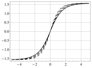
where B4γab2/(43α)𝐵4𝛾𝑎superscript𝑏243𝛼B\equiv 4\gamma ab^{2}/(4-3\alpha). In Fig. 1 we depict the behavior of the solution (34). We note that the thickness of the solution is controlled essentially by α𝛼\alpha. Moreover, as expected, the solution goes to the asymptotic value ϕϕ¯=±π/2bitalic-ϕ¯italic-ϕplus-or-minus𝜋2𝑏\phi\to\bar{\phi}=\pm\pi/2b when y±𝑦plus-or-minusy\to\pm\infty.

Refer to caption
Figure 1: The solution (34), depicted for a=b=γ=1𝑎𝑏𝛾1a=b=\gamma=1 and α=0𝛼0\alpha\!=\!0 (solid line), α=0.1,0.2,0.3,0.4𝛼0.10.20.30.4\alpha\!=\!0.1,0.2,0.3,0.4 (dashed lines).

Using equation (28) we can also get the warp function as

A(y)=2γa3Bln[sech(By)].𝐴𝑦2𝛾𝑎3𝐵sech𝐵𝑦A(y)=\frac{2\gamma a}{3B}~{}\ln\Big{[}\mbox{sech}(By)\Big{]}\,. (35)

If α<4/3𝛼43\alpha<4/3 we can get the thin-brane limit when y±𝑦plus-or-minusy\to\pm\infty, in the form

A(y±)2γa3|y|.𝐴𝑦plus-or-minus2𝛾𝑎3𝑦A(y\to\pm\infty)\backsim-\frac{2\gamma a}{3}|y|\,. (36)

In Fig. 2 we depict the warp factor e2Asuperscript𝑒2𝐴e^{2A} for some values of the parameters. We note that the warp factor narrows as α𝛼\alpha increases.

Refer to caption
Figure 2: The warp factor e2Asuperscript𝑒2𝐴e^{2A}, depicted for a=b=γ=1𝑎𝑏𝛾1a=b=\gamma=1 and α=0𝛼0\alpha\!=\!0 (solid line), and for α=0.1,0.2,0.3,0.4𝛼0.10.20.30.4\alpha\!=\!0.1,0.2,0.3,0.4 (dashed lines).

Furthermore, the potential (30) can be written as

V(ϕ)=16(aγ)23(45α)+2γa(3B+8γa)3(45α)cos2(bϕ),𝑉italic-ϕ16superscript𝑎𝛾2345𝛼2𝛾𝑎3𝐵8𝛾𝑎345𝛼superscript2𝑏italic-ϕV(\phi)=-\frac{16(a\gamma)^{2}}{3(4\!-\!5\alpha)}+\frac{2\gamma a(3B+8\gamma a)}{3(4\!-\!5\alpha)}\cos^{2}(b\phi)\,, (37)

which is depicted in Fig. 3. Note that the potential has several global minima at ϕ=ϕ¯iitalic-ϕsubscript¯italic-ϕ𝑖\phi=\bar{\phi}_{i}, where

V(ϕ¯i)=163(aγ)2(45α).𝑉subscript¯italic-ϕ𝑖163superscript𝑎𝛾245𝛼V(\bar{\phi}_{i})=-\frac{16}{3}\frac{(a\gamma)^{2}}{(4-5\alpha)}\,. (38)
Refer to caption
Figure 3: The scalar field potential, depicted for a=b=γ=1𝑎𝑏𝛾1a=b=\gamma=1 and α=0𝛼0\alpha\!=\!0 (solid line), α=0.1,0.2,0.3,0.4𝛼0.10.20.30.4\alpha\!=\!0.1,0.2,0.3,0.4 (dashed lines).

Finally, the energy density (31) can be written as

ρ(y)𝜌𝑦\displaystyle\rho(y)\!\!\! =\displaystyle= 16(γa)23(45α)[1+(1+3B(1α)γa(43α))sech2(By)]×\displaystyle\!\!\!\frac{16(\gamma a)^{2}}{3(4\!-\!5\alpha)}\!\Big{[}\!\!-\!1\!+\!\!\Big{(}\!1\!+\!\frac{3B(1\!-\!\alpha)}{\gamma a(4\!-\!3\alpha)}\!\Big{)}\mbox{sech}^{2}(By)\!\Big{]}\!\!\times (39)
×[sech(By)]4γa3B.absentsuperscriptdelimited-[]sech𝐵𝑦4𝛾𝑎3𝐵\displaystyle\!\!\!\times\Big{[}\mbox{sech}(By)\Big{]}^{\frac{4\gamma a}{3B}}\,.

Fig. 4 shows how the parameter α𝛼\alpha controls the energy density. The equation (39) can be integrated to give the energy of the brane in the form

Eα=αB4b2(89α45α)πΓ(s)Γ(s+1/2),subscript𝐸𝛼𝛼𝐵4superscript𝑏289𝛼45𝛼𝜋Γ𝑠Γ𝑠12E_{\alpha}=\alpha\frac{B}{4b^{2}}\Big{(}\frac{8\!-\!9\alpha}{4\!-\!5\alpha}\Big{)}~{}\frac{\sqrt{\pi}~{}\Gamma\left(s\right)}{\Gamma(s+1/2)}\,, (40)

where s1+2γa/3B𝑠12𝛾𝑎3𝐵s\equiv 1+2\gamma a/3B.

Refer to caption
Figure 4: The energy density, depicted for a=b=γ=1𝑎𝑏𝛾1a=b=\gamma=1 and α=0𝛼0\alpha\!=\!0 (solid line), and for α=0.1,0.2,0.3,0.4𝛼0.10.20.30.4\alpha\!=\!0.1,0.2,0.3,0.4 (dashed lines).

The behavior of the stability of the gravitational sector can be analyzed analytically for the particular case where B=2γa/3𝐵2𝛾𝑎3B=2\gamma a/3. In this case we can make the change

y=1Barcsinh(Bz).𝑦1𝐵arcsinh𝐵𝑧y=\frac{1}{B}\mbox{arcsinh}(Bz)\,. (41)

With this we get the stability potential in the form

U(z)=3B2425B2z2(1+B2z2)2.𝑈𝑧3superscript𝐵2425superscript𝐵2superscript𝑧2superscript1superscript𝐵2superscript𝑧22U(z)=-\frac{3B^{2}}{4}\frac{2-5B^{2}z^{2}}{\left(1+B^{2}z^{2}\right)^{2}}\,. (42)

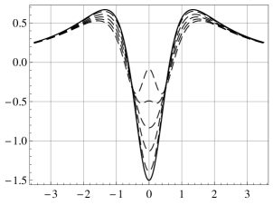
It is depicted in Fig. 5, for several values of the parameters.
Refer to caption
Figure 5: The stability potential, depicted for B=2/3𝐵23B\!=\!2/3 (solid line), and for B=1,4/3,5/3𝐵14353B\!=\!1,4/3,5/3 (dashed lines).

The above results show that the thick brane narrows as α𝛼\alpha increases, but the brane profile is qualitatively similar to the case of a standard brane.

III.2 Another model

Let us go on and investigate another model, this time with contribution from the Ricci scalar too. We assume that

F(R,T)=R+βR2αT,𝐹𝑅𝑇𝑅𝛽superscript𝑅2𝛼𝑇F(R,T)=R+\beta R^{2}-\alpha T\,, (43)

where α𝛼\alpha and β𝛽\beta are real parameters. The case with α=0𝛼0\alpha=0 has been studied in Bazeia:2013uva , and now we add both the R2superscript𝑅2R^{2} and T𝑇T contributions, to get analytical results. In Ref. Bazeia:2013uva one noted that the term R2superscript𝑅2R^{2} contributes to generate an interesting effect, the splitting of the brane, and here we want to see how it works. In this new model, the brane equations become

43α6ϕ2=A′′+8β3(2A′′′′+16A′′2+8AA′′′+5A2A′′),43𝛼6superscriptitalic-ϕ2superscript𝐴′′8𝛽32superscript𝐴′′′′16superscript𝐴′′28superscript𝐴superscript𝐴′′′5superscript𝐴2superscript𝐴′′\displaystyle\!-\frac{4\!-\!3\alpha}{6}\phi^{\prime 2}\!\!=\!\!A^{\prime\prime}\!\!+\!\frac{8\beta}{3}\Big{(}\!2A^{\prime\prime\prime\prime}\!\!+\!16A^{\prime\prime 2}\!\!+\!8A^{\prime}\!\!A^{\prime\prime\prime}\!\!+\!5A^{\prime 2}\!\!A^{\prime\prime}\!\Big{)},
(44a)
43α24ϕ245α12V=A2+43𝛼24superscriptitalic-ϕ245𝛼12𝑉limit-fromsuperscript𝐴2\displaystyle\frac{4-3\alpha}{24}\phi^{\prime 2}-\frac{4-5\alpha}{12}V=A^{\prime 2}+\quad\quad\quad\quad\quad\quad\quad~{}~{}~{}~{}
+4β3(5A4+8AA′′′+32A2A′′4A′′2).4𝛽35superscript𝐴48superscript𝐴superscript𝐴′′′32superscript𝐴2superscript𝐴′′4superscript𝐴′′2\displaystyle+\frac{4\beta}{3}\Big{(}5A^{\prime 4}\!\!+8A^{\prime}A^{\prime\prime\prime}\!\!+32A^{\prime 2}A^{\prime\prime}\!\!-4A^{\prime\prime 2}\Big{)}.~{}~{}~{} (44b)

We note that if β=0𝛽0\beta=0 we get to the equations (27). Also, for β0𝛽0\beta\neq 0 the equations involve the fourth derivative of the warp function, which makes it difficult to search for solutions. However, as suggested in Bazeia:2013uva if we choose the warp function A(y)𝐴𝑦A(y) as

A(y)=ln[sech(ky)],𝐴𝑦sech𝑘𝑦A(y)=\ln\Big{[}\mbox{sech}(ky)\Big{]}\,, (45)

where k𝑘k is a positive parameter, this allows us to write the relations (44) as

ϕ2superscriptitalic-ϕ2\displaystyle\phi^{\prime 2}\!\!\! =\displaystyle= 6k243αS2+16βk443αS2(2949S2),6superscript𝑘243𝛼superscript𝑆216𝛽superscript𝑘443𝛼superscript𝑆22949superscript𝑆2\displaystyle\!\!\!\frac{6k^{2}}{4-3\alpha}S^{2}\!+\!\frac{16\beta k^{4}}{4-3\alpha}S^{2}\Big{(}29-49S^{2}\Big{)}\,, (46a)
V(y)𝑉𝑦\displaystyle V(y)\!\!\! =\displaystyle= 12k245α+15k245αS28βk445α(10145S2+147S4),12superscript𝑘245𝛼15superscript𝑘245𝛼superscript𝑆28𝛽superscript𝑘445𝛼10145superscript𝑆2147superscript𝑆4\displaystyle\!\!\!-\frac{12k^{2}}{4\!-\!5\alpha}\!+\!\frac{15k^{2}}{4\!-\!5\alpha}S^{2}\!-\!\frac{8\beta k^{4}}{4\!-\!5\alpha}\Big{(}\!10\!-\!145S^{2}\!\!+\!147S^{4}\!\Big{)}\,,

where S=sech(ky)𝑆sech𝑘𝑦S=\mbox{sech}(ky). We use equation (46a) to see that β𝛽\beta should be limited to the interval

3232k2β3160k2.3232superscript𝑘2𝛽3160superscript𝑘2-\frac{3}{232k^{2}}\leq\beta\leq\frac{3}{160k^{2}}\,. (47)

Moreover, we suppose that the parameter α𝛼\alpha is positive, smaller than 4/5454/5. For this model, we can write the energy density as

ρ(y)𝜌𝑦\displaystyle\rho(y)\!\! =\displaystyle= 12k245αS2+12k2(65α)(43α)(45α)S48βk445αS2[10\displaystyle\!\!-\frac{12k^{2}}{4\!-\!5\alpha}S^{2}\!+\!\frac{12k^{2}(6\!-\!5\alpha)}{(4\!-\!3\alpha)(4\!-\!5\alpha)}S^{4}\!-\!\frac{8\beta k^{4}}{4\!-\!5\alpha}S^{2}\Big{[}10- (48)
116(65α)43αS2+98(87α)43αS4].\displaystyle\!-\frac{116(6-5\alpha)}{4\!-\!3\alpha}S^{2}\!+\!\frac{98(8-7\alpha)}{4\!-\!3\alpha}S^{4}\Big{]}\,.

A closer examination of the energy density (48) shows that it start to split when

β=3(87α)16(125116α)k2.𝛽387𝛼16125116𝛼superscript𝑘2\beta=\frac{3(8-7\alpha)}{16(125-116\alpha)k^{2}}\,. (49)

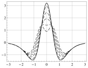
The splitting depends on α𝛼\alpha, so the modification introduced with the presence of T𝑇T contributes to control this effect. In Fig. 6 we depict the energy density for k=1𝑘1k=1, α=1/2𝛼12\alpha\!=\!1/2 and β𝛽\beta within the interval (47). In this case the split starts approximately at β=0.012𝛽0.012\beta=0.012.

Refer to caption
Figure 6: The energy density, depicted for k=1𝑘1k=1, α=1/2𝛼12\alpha=1/2 and β=0𝛽0\beta\!=\!0 (solid line), β=0.002,0.006,0.010,0.014,0.018𝛽0.0020.0060.0100.0140.018\beta\!=\!0.002,0.006,0.010,0.014,0.018 (dashed lines).
Refer to caption
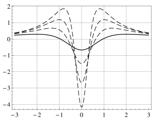
Figure 7: The stability potential, depicted for k=1𝑘1k=1 and β=0𝛽0\beta\!=\!0 (solid line), β=0.002,0.006,0.010,0.014,0.018𝛽0.0020.0060.0100.0140.018\beta\!=\!0.002,0.006,0.010,0.014,0.018 (dashed lines).

The solutions of equation (46a) can be written as

ϕ(y)=±643α320βk243αEllipticE(ϕs;392βk2160βk23),italic-ϕ𝑦plus-or-minus643𝛼320𝛽superscript𝑘243𝛼EllipticEsubscriptitalic-ϕ𝑠392𝛽superscript𝑘2160𝛽superscript𝑘23\phi(y)=\pm\sqrt{\frac{6}{4\!-\!3\alpha}\!-\!\frac{320\beta k^{2}}{4-3\alpha}}~{}\mbox{EllipticE}~{}\Big{(}\phi_{s};\frac{392\beta k^{2}}{160\beta k^{2}\!-\!3}\Big{)}\,, (50)

where ϕs=arcsin[tanh(ky)]subscriptitalic-ϕ𝑠𝑘𝑦\phi_{s}=\arcsin\Big{[}\tanh(ky)\Big{]} and EllipticE is the elliptic integral of the second kind. For β=3/232k2𝛽3232superscript𝑘2\beta=-3/232k^{2} and β=0𝛽0\beta=0 we obtain the solution as, respectively,

ϕ(y)italic-ϕ𝑦\displaystyle\phi(y) =\displaystyle= 29411687αtanh(ky),29411687𝛼𝑘𝑦\displaystyle\sqrt{\frac{294}{116-87\alpha}}~{}\tanh(ky)\,, (51a)
ϕ(y)italic-ϕ𝑦\displaystyle\phi(y) =\displaystyle= 643αarcsin[tanh(ky)].643𝛼𝑘𝑦\displaystyle\sqrt{\frac{6}{4-3\alpha}}\arcsin\Big{[}\tanh(ky)\Big{]}\,. (51b)

We now study linear stability of the gravity sector. For this we make the following change of variables

y=1karcsinh(kz).𝑦1𝑘arcsinh𝑘𝑧y=\frac{1}{k}\mbox{arcsinh}(kz)\,. (52)

It allows to get the stability potential as

U(z)𝑈𝑧\displaystyle U(z)\!\!\! =\displaystyle= 3k2425k2z2(1+k2z2)2+56βk4(13k2z2)(1+k2z2)2f(z)3superscript𝑘2425superscript𝑘2superscript𝑧2superscript1superscript𝑘2superscript𝑧22limit-from56𝛽superscript𝑘413superscript𝑘2superscript𝑧2superscript1superscript𝑘2superscript𝑧22𝑓𝑧\displaystyle\!\!\!-\frac{3k^{2}}{4}\frac{2-5k^{2}z^{2}}{(1+k^{2}z^{2})^{2}}+\frac{56\beta k^{4}(1-3k^{2}z^{2})}{(1+k^{2}z^{2})^{2}f(z)}- (53)
3136k8z2β2(1+k2z2)2f(z)2,3136superscript𝑘8superscript𝑧2superscript𝛽2superscript1superscript𝑘2superscript𝑧22𝑓superscript𝑧2\displaystyle\!\!\!-\frac{3136k^{8}z^{2}\beta^{2}}{(1+k^{2}z^{2})^{2}f(z)^{2}}\,,

where, f(z)=1+k2z28βk2(25k2z2)𝑓𝑧1superscript𝑘2superscript𝑧28𝛽superscript𝑘225superscript𝑘2superscript𝑧2f(z)=1+k^{2}z^{2}-8\beta k^{2}(2-5k^{2}z^{2}). This potential is depicted in Fig. 7. The appearance of a lump in the well confirms the splitting of the brane as β𝛽\beta increases. We note that the stability potential does not depend on α𝛼\alpha, although α𝛼\alpha contributes to split the brane, as shown above in (49), for instance.

The results show that the presence of R2superscript𝑅2R^{2} controls the splitting of the brane, as also noted in Ref. Bazeia:2013uva ; here, however, the T𝑇T term also contributes, adding quantitative modification to the braneworld profile.

We can also consider adding a quadratic term in T𝑇T with a quadratic term in the scalar curvature. In this case, we have

F=R+βR2αT2.𝐹𝑅𝛽superscript𝑅2𝛼superscript𝑇2F=R+\beta R^{2}-\alpha T^{2}\,. (54)

The equations (9) become

23ϕ2+αϕ2T=23superscriptitalic-ϕ2𝛼superscriptitalic-ϕ2𝑇absent\displaystyle-\frac{2}{3}\phi^{\prime 2}+\alpha\phi^{\prime 2}T=
A′′+83β(2A′′′′+16A′′2+8AA′′′+5A2A′′),superscript𝐴′′83𝛽2superscript𝐴′′′′16superscript𝐴′′28superscript𝐴superscript𝐴′′′5superscript𝐴2superscript𝐴′′\displaystyle A^{\prime\prime}+\frac{8}{3}\beta\Big{(}\!2A^{\prime\prime\prime\prime}\!\!+\!16A^{\prime\prime 2}\!\!+\!8A^{\prime}\!\!A^{\prime\prime\prime}\!\!+\!5A^{\prime 2}\!\!A^{\prime\prime}\Big{)}\,, (55a)
V(ϕ)12ϕ2+3α2ϕ2Tα4T2=𝑉italic-ϕ12superscriptitalic-ϕ23𝛼2superscriptitalic-ϕ2𝑇𝛼4superscript𝑇2absent\displaystyle\!\!\!\!\!\!V(\phi)\!-\!\frac{1}{2}\phi^{\prime 2}+\!\frac{3\alpha}{2}\phi^{\prime 2}T-\frac{\alpha}{4}T^{2}=
3A24β(5A4+8AA′′′+32A2A′′4A′′2).3superscript𝐴24𝛽5superscript𝐴48superscript𝐴superscript𝐴′′′32superscript𝐴2superscript𝐴′′4superscript𝐴′′2\displaystyle-3A^{\prime 2}-4\beta\Big{(}5A^{\prime 4}\!\!+8A^{\prime}A^{\prime\prime\prime}\!\!+32A^{\prime 2}A^{\prime\prime}\!\!-4A^{\prime\prime 2}\Big{)}.\;\;\;\; (55b)

To solve the model we assume that the warp function is yet given by (45), and we take k=1𝑘1k=1. This problem is much harder then the previous one, but we then rewrite the above equations in the simpler form

ϕ23α2ϕ2T=32S2+4β(29S249S4),superscriptitalic-ϕ23𝛼2superscriptitalic-ϕ2𝑇32superscript𝑆24𝛽29superscript𝑆249superscript𝑆4\displaystyle\phi^{\prime 2}-\frac{3\alpha}{2}\phi^{\prime 2}T=\frac{3}{2}S^{2}+4\beta\Big{(}29S^{2}-49S^{4}\Big{)}, (56a)
V(ϕ)12ϕ2+3α2ϕ2Tα4T2=𝑉italic-ϕ12superscriptitalic-ϕ23𝛼2superscriptitalic-ϕ2𝑇𝛼4superscript𝑇2absent\displaystyle V(\phi)\!-\!\frac{1}{2}\phi^{\prime 2}+\!\frac{3\alpha}{2}\phi^{\prime 2}T-\frac{\alpha}{4}T^{2}=
3+3S24β(558S2+49S4).33superscript𝑆24𝛽558superscript𝑆249superscript𝑆4\displaystyle\;\;\;\;\;\;\;\;\;\;-3+3S^{2}-4\beta\Big{(}5-58S^{2}+49S^{4}\Big{)}. (56b)

These equations have analytical solutions for appropriate choices of the parameters α𝛼\alpha and β𝛽\beta. We have examined some specific cases, and they are all similar. Thus, we take, for instance, α=0.02304𝛼0.02304\alpha=0.02304 and β=0.00433𝛽0.00433\beta=0.00433; the solutions are

ϕ(y)italic-ϕ𝑦\displaystyle\phi(y)\!\! =\displaystyle= ±parcsin[tanh(y)],plus-or-minus𝑝𝑦\displaystyle\!\!\pm\,p\arcsin[\tanh(y)]\,, (57a)
V(ϕ)𝑉italic-ϕ\displaystyle V(\phi)\!\! =\displaystyle= 2.31489+3.00269cos2(ϕp),2.314893.00269superscript2italic-ϕ𝑝\displaystyle\!\!-2.31489+3.00269\cos^{2}\Big{(}\frac{\phi}{p}\Big{)}\,, (57b)

where p=1.19576𝑝1.19576p=1.19576. The energy density becomes

ρ(y)=2.31489S2+3.71762S4.𝜌𝑦2.31489superscript𝑆23.71762superscript𝑆4\rho(y)=-2.31489\,S^{2}+3.71762\,S^{4}\,. (58)

It is depicted in Fig 8, showing standard profile. The absence of splitting is due to the fact that the analytical solution is obtained for a very small value of β𝛽\beta.

Refer to caption
Figure 8: The energy density, depicted for the solution (58).

IV COMMENTS AND CONCLUSIONS

In this work we studied some thick braneworld scenarios in an AdS5𝐴𝑑subscript𝑆5AdS_{5} warped geometry with a single extra dimension of infinite extent, with the gravity sector extended to accommodate the F(R,T)𝐹𝑅𝑇F(R,T) modification, coupled to a single real scalar field with standard kinematics. We used the equations of motion to show explicitly that the gravity sector is linearly stable when we consider F(R,T)=G(R)+H(T)𝐹𝑅𝑇𝐺𝑅𝐻𝑇F(R,T)=G(R)+H(T).

We investigated two distinct models, the first one with F(R,T)=RαT𝐹𝑅𝑇𝑅𝛼𝑇F(R,T)=R-\alpha\,T, and the other with F(R,T)=R+βR2αT𝐹𝑅𝑇𝑅𝛽superscript𝑅2𝛼𝑇F(R,T)=R+\beta R^{2}-\alpha T. In the first case, the contributions that appear from the extra term T𝑇T induces quantitative modifications in the thick brane profile, without changing its qualitative behavior. In the second case, the presence of R2superscript𝑅2R^{2} works to split the brane. This effect was identified before in Bazeia:2013uva , and the modification introduced with αT𝛼𝑇\alpha\,T also contributes to the splitting, but it adds no new effect in the braneworld profile. We then conclude that the modification of the form RF(R,T)=G(R)+H(T)𝑅𝐹𝑅𝑇𝐺𝑅𝐻𝑇R\to F(R,T)=G(R)+H(T) does not destabilize the gravity sector of the thick braneworld with an AdS5𝐴𝑑subscript𝑆5AdS_{5} warped geometry with a single extra dimension of infinite extent. Moreover, the presence of the term H(T)=αT𝐻𝑇𝛼𝑇H(T)=-\alpha\,T contributes to change the braneworld profile quantitatively, although it adds no new qualitative effect to the brane. If we add the term H(T)=αT2𝐻𝑇𝛼superscript𝑇2H(T)=-\alpha T^{2}, it seems that the effect is similar, but here, however, one needs to explore a larger range of parameters. This task requires numerical investigation, an issue that is out of the scope of the work.

The present study drives our attention to some issues of current interest, one concerning the investigation of how the quantitative modifications that we have identified in this work act to localize fermion and gauge fields within the thick brane fl ; gl . Another, very natural continuation is related to the hybrid brane recently proposed, in which one changes the potential of the source field to make the scalar field solution compact we2 , to see how it adds in this new scenario. This last issue is now under consideration, and we hope to report on it in the near future.

Acknowledgements.
DB and RM would like to thank CNPq for partial financial support.

References

  • (1)
  • (2) L. Randall and R. Sundrum, Phys. Rev. Lett. 83, 4690 (1999).
  • (3) W.D. Goldberger and M.B. Wise, Phys. Rev. Lett. 83, 4922 (1999).
  • (4) O. DeWolfe, D. Z. Freedman, S. S. Gubser and A. Karch, Phys. Rev. D 62, 046008 (2000).
  • (5) C. Csaki, J. Erlich, T. Hollowood, Y. Shirman, Nucl. Phys. B 581, 309 (2000); C. Csaki, J. Erlich, G. Grojean, T. Hollowood, Nucl. Phys. B 584, 359 (2000).
  • (6) M. Gremm, Phys. Lett. B 478, 434 (2000); F.A. Brito, M. Cvetic, and S.-C. Yoon, Phys. Rev. D 64, 064021 (2001); M. Cvetic and N.D. Lambert, Phys. Lett. B 540, 301 (2002); A. Campos, Phys. Rev. Lett. 88, 141602 (2002); A. Melfo, N. Pantoja, and A. Skirzewski, Phys. Rev. D 67, 105003 (2003); D. Bazeia, F.A. Brito, and J.R. Nascimento, Phys. Rev. D 68, 085007 (2003); D. Bazeia, C. Furtado, and A.R. Gomes, JCAP 0402, 002 (2004); D. Bazeia and A.R. Gomes, JHEP 0405, 012 (2004).
  • (7) C.M. Will, Living Rev. Rel. 9, 3 (2006); R.P. Woodard, Lect. Notes Phys. 720, 403 (2007).
  • (8) P. Pani, T.P. Sotiriou and D. Vernieri, Phys. Rev. D 88, 121502 (2013).
  • (9) T.P. Sotiriou and V. Faraoni, Rev. Mod. Phys. 82 451 (2010); A. De Felice, S. Tsujikawa, Living Rev. Rel. 13, 3 (2010).
  • (10) T. Harko, F. S. N. Lobo and E. N. Saridakis, Cosmology with higher-derivative matter fields. arXiv:1405.7019.
  • (11) D. Bazeia, F.A. Brito, and F.G. Costa, Phys. Rev. D 90, 043523 (2014).
  • (12) Bin Guo, Yu-Xiao Liu, and Ke Yang, Brane worlds in gravity with auxiliary fields. arXiv:1405.0074.
  • (13) D. Bazeia, A.S. Lobão Jr., and R. Menezes, Phys. Rev. D 90 (2014); D. Bazeia, M.A. Marques, R. Menezes, and D.C. Moreira, New braneworld models in the presence of auxiliary fields, arXiv:1412.XXXX.
  • (14) Yu-Xiao Liu, Yuan Zhong, Zhen-Hua Zhao, Hai-Tao Li, JHEP 1106, 135 (2011).
  • (15) Yi Zhong, Yu-Xiao Liu, Feng-Wei Chen, Qun-Ying Xie, Warped Brane worlds in Critical Gravity, arXiv:1403.5109; Zeng-Guang Xu, Yu-Xiao Liu, Yuan Zhong, Metastable gravitons in f(R)𝑓𝑅f(R)-brane models, arXiv:1405.6277; D. Bazeia, L. Losano, R. Menezes, G.J. Olmo, and D. Rubiera-Garcia, Thick brane in f(R)𝑓𝑅f(R) gravity with Palatini dynamics, arXiv:1411.0897.
  • (16) T. Harko, F. S. N. Lobo, S. Nojiri and S. D. Odintsov, Phys. Rev. D 84, 024020 (2011).
  • (17) F. G. Alvarenga, A. de la Cruz-Dombriz, M. J. S. Houndjo, M. E. Rodrigues and D. Sáez-Gómez, Phys. Rev. D 87, 103526 (2013).
  • (18) D. Bazeia, A. S. Lobão Jr., R. Menezes, A. Y. Petrov and A. J. da Silva, Phys. Lett. B 729, 127 (2014).
  • (19) R.A.C. Correa, A. de Souza Dutra, and M.B. Hott, Class. Quant. Grav. 28, 155012 (2011); A.E.R. Chumbes, A.E.O. Vasquez, and M.B. Hott, Phys. Rev. D 83, 105010 (2011); Yu-Xiao Liu, Zeng-Guang Xu, Feng-Wei Chen, and Shao-Wen Wei, Phys. Rev. D 89, 086001 (2014).
  • (20) W.T. Cruz, A.R.P. Lima, C.A.S. Almeida, Phys. Rev. D, 87, 045018 (2013); W.T. Cruz, R.V. Maluf, C.A.S. Almeida, Eur. Phys. J. C 73, 2423 (2013).
  • (21) D. Bazeia, L. Losano, M.A. Marques, and R. Menezes, EPL 107, 61001 (2014); Phys. Lett. B 736, 515 (2014).