First High-resolution Spectroscopic Observations of an Erupting Prominence Within a Coronal Mass Ejection by the Interface Region Imaging Spectrograph (IRIS)
Abstract
Spectroscopic observations of prominence eruptions associated with coronal mass ejections (CMEs), although relatively rare, can provide valuable plasma and 3D geometry diagnostics. We report the first observations by the Interface Region Imaging Spectrograph (IRIS) mission of a spectacular fast CME/prominence eruption associated with an equivalent X1.6 flare on 2014 May 9. The maximum plane-of-sky and Doppler velocities of the eruption are 1200 and , respectively. There are two eruption components separated by in Doppler velocity: a primary, bright component and a secondary, faint component, suggesting a hollow, rather than solid, cone-shaped distribution of material. The eruption involves a left-handed helical structure undergoing counter-clockwise (viewed top-down) unwinding motion. There is a temporal evolution from upward eruption to downward fallback with less-than-free-fall speeds and decreasing nonthermal line widths. We find a wide range of Mg II k/h line intensity ratios (less than 2 expected for optically-thin thermal emission): the lowest ever-reported median value of 1.17 found in the fallback material and a comparably high value of 1.63 in nearby coronal rain and intermediate values of 1.53 and 1.41 in the two eruption components. The fallback material exhibits a strong () linear correlation between the k/h ratio and the Doppler velocity as well as the line intensity. We demonstrate that Doppler dimming of scattered chromospheric emission by the erupted material can potentially explain such characteristics.
Subject headings:
Sun: activity—Sun: corona—Sun: coronal mass ejections—Sun: filaments, prominences—Sun: UV radiation1. Introduction
As one of the major drivers of space-weather disturbances, coronal mass ejections (CMEs; see Chen, 2011; Webb & Howard, 2012, for recent reviews) are powerful eruptions of typically – masses from the Sun traveling at 100 – and involving energies of – . CMEs seen in white light often exhibit a classic three-part morphology (e.g., Hundhausen et al., 1984; Schwenn, 1996) consisting of a bright leading front surrounding a dark cavity containing a bright core. The core is identified as an erupting prominence (e.g., Tandberg-Hanssen, 1995; Martin, 1998; Labrosse et al., 2010; Mackay et al., 2010; Parenti, 2014), some cool () and dense “chromospheric” plasma residing in the hot () and tenuous corona prior to its eruption.
Prominence eruptions and CMEs in general are conventionally detected with global imaging instruments, which can constrain the morphology and plane-of-sky (POS) velocity among other observables. Such observations are obtained either monochromatically (e.g., in H, extreme ultraviolet [EUV], or white light; St. Cyr et al. 2000) or in multiple passbands (e.g., with the Coronal Multichannel Polarimeter [CoMP]; Tian et al. 2013).
Spectroscopic observations of prominence eruptions or CMEs within restricted fields of view (FOVs) of slit spectrographs, although comparably rare, can provide valuable, complementing plasma diagnostics, e.g., density, temperature, and Doppler velocity. Such observations were obtained (i) in the outer corona (1.4 – ) by the UltraViolet Coronagraph Spectrometer (UVCS; e.g., Ciaravella et al., 1997; Raymond et al., 2003) onboard the Solar and Heliospheric Observatory (SOHO), and (ii) in the inner corona () by spectroheliographs on Skylab (e.g., Schmahl & Hildner, 1977; Widing et al., 1986), the Ultraviolet Spectrometer and Polarimeter (UVSP) on the Solar Maximum Mission (SMM; e.g., Fontenla & Poland, 1989), the Solar Ultraviolet Measurements of Emitted Radiation (SUMER) and Coronal Diagnostic Spectrometer (CDS) on SOHO (e.g., Wiik et al., 1997), the EUV Imaging Spectrometer (EIS) on Hinode (e.g., Harra et al. 2007; Jin et al. 2009; Tian et al. 2012; Williams et al. 2015, in prep.), and ground-based instruments (e.g., Penn, 2000). Notably, during 1996 – 2005, UVCS detected 1000 CMEs (Giordano et al., 2013), about 10% of the CMEs detected by the SOHO Large Angle and Spectrometric Coronagraph (LASCO) during the same period. The most commonly detected feature of UVCS CMEs (in 70% of them) is the cool prominence material.
The recently launched Interface Region Imaging Spectrograph mission (IRIS; De Pontieu et al., 2014), thanks to its advanced capabilities over previous generations of instruments, has provided a new opportunity to observe CMEs and especially prominence eruptions in unprecedented detail. IRIS offers a high resolution of – in space, in time, and in Doppler velocity. A unique advantage of IRIS is the combination of spectra and slit-jaw images (SJIs), which provides simultaneous Doppler and POS velocity measurement and can thus constrain the true three-dimensional (3D) geometry and velocity vector. Its ultraviolet (UV) spectra cover a wide temperature range of – and are particularly sensitive to chromospheric and transition-region temperatures of prominence material. With its FOV covering the low corona, IRIS can provide critical clues to the initiation and early development of a CME/prominence eruption and complement instruments covering the high corona (e.g., coronagraphs and UVCS which was turned off on 2012 December 15).
We report in this paper the first result of IRIS observations of an erupting prominence within a CME. We present the overview of observations in Section 2, data analysis results in Section 3, and concluding remarks in Section 4.
2. Overview of Observations
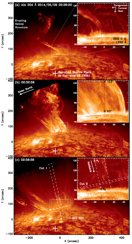
On 2014 May 9, a major eruption involving a flare and a CME with a prominence eruption occurred in NOAA active region (AR) 12051 on the far side of the Sun. The flare kernel, observed by the Extreme UltraViolet Imager (EUVI) on the Solar TErrestrial RElations Observatory Ahead spacecraft (STEREO-A), was located behind the west limb seen from the Earth perspective. Its POS projection, shown as the plus sign in 1(a), was located at (, ), inside the limb. The pre-event background removed full-disk EUVI 195 Å flux (1(d), blue line, at a 5 min cadence) peaked at 02:21 UT and , which translates to an equivalent GOES X-ray flare class of X1.6, according to empirical scaling (Nitta et al., 2013). The CME observed by SOHO/LASCO had a maximum POS speed of , according to the CACTUS catalog (http://sidc.oma.be/cactus).
As seen by the Atmospheric Imaging Assembly (AIA) on the Solar Dynamics Observatory (SDO) in the He II 304 Å channel, the prominence eruption occurred in two episodes starting at 02:20 and 02:28 UT, with leading-edge speeds of 1060 and , respectively. Episode 1 involved a single helical material thread expanding radially (1(a)). Episode 2 was more complex, consisting of sub-structured material bundles spanning a cone shape up to in angular extent (Figures 1(b) and (c)), whose central axis (along “Cut 1”) was oriented counter-clockwise from the radial direction. Episode 2 lasted more than an hour up to 03:45 UT, with material being episodically ejected in some directions and at the same time falling back to the Sun in some other directions.
IRIS was running large coarse 8-step rasters with a step size of and 9.6 s cadence (8 s exposure) through 03:21 UT. SJIs in a single C II 1330 Å channel (bandwidth: 55 Å) covered a maximum FOV, as shown in 1(c). The IRIS slit, oriented at clockwise from the eruption axis, missed the first episode but fully covered the second, which will be the focus of this paper. Table 1 summarizes the milestones of this event and corresponding coverage by different instruments.
| 02:16/02:21 | Flare onset/peak seen by STEREO-A (5 min cadence) |
|---|---|
| 02:18 | EUV wave onset seen by SDO/AIA |
| 02:20–02:28 | Prominence eruption Episode 1 seen by SDO/AIA |
| Max. POS speed at 02:21 | |
| 02:28–03:45 | Prominence eruption Episode 2 seen by SDO/AIA |
| Max. POS speed at 02:29 | |
| 02:28–03:21 | IRIS slit coverage of Episode 2 eruption |
| Max. redshift at 02:31 | |
| 02:48 | CME seen by SOHO/LASCO (24 min cadence) |
| 02:50 | Transition from eruption to fallback within IRIS slit |
3. IRIS Data Analysis
3.1. Wavelength Calibration
We performed on IRIS level-2 data relative (not absolute) wavelength calibration, which practically served our purpose of measuring the Doppler velocity of the eruption. Shown as the vertical dotted line in 2, the reference wavelength for the Doppler velocity in each spectral line window was selected at the centroid of the corresponding line profile averaged over the on-disk portion of the slit through this event (02:17–03:21 UT). Therefore, all the Doppler velocities are measured with respect to the quiet-Sun region near the limb within the IRIS slit, which is located in the neighborhood of the eruption source region (the plus sign in 1(a)).
The absolute uncertainty of this relative wavelength calibration can be estimated as follows. Taking the Mg II k 2796 Å line as an example, the sources of uncertainty include (i) the wavelength shift (equivalent to ) of this line measured near the solar limb from that at the disk center (Kohl & Parkinson, 1976) and (ii) the IRIS orbital thermal variation of (De Pontieu et al., 2014). These errors combined give an overall uncertainty of for the absolute Doppler velocity, two orders of magnitude smaller than the typical values of hundreds of measured in this eruption.
3.2. Temperature Distribution
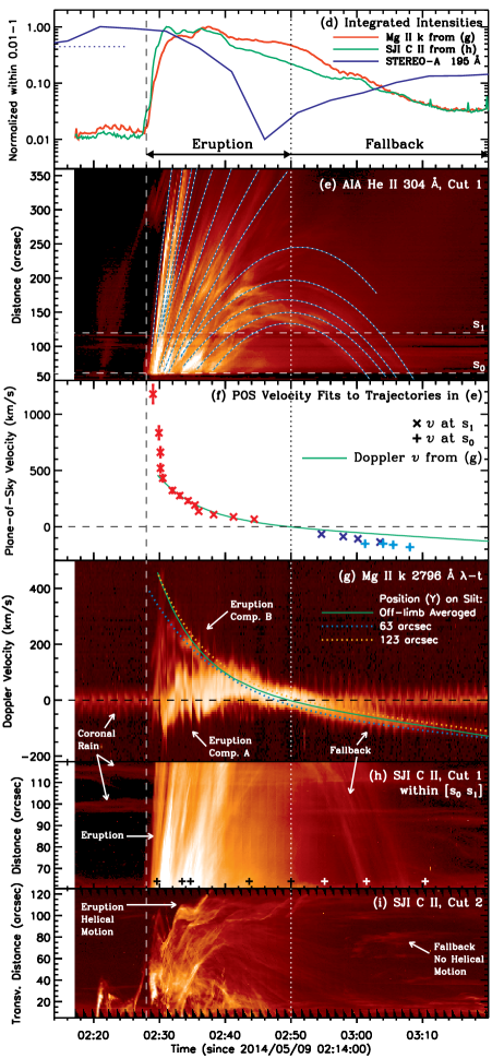
The eruption was observed in C II 1330 Å SJIs and spectra of cool lines at chromospheric to transition region temperatures, including Mg II (), C II (), Si IV (), and O IV (), as shown in 2, corresponding to the erupting prominence material. IRIS detected no eruption-associated signal in the Fe XII 1349 Å () or Fe XXI 1354 Å () line, although AIA detected in its Fe XII 193 Å and Fe XIV 211 Å () channels a dome-shaped, CME-generated EUV wave (e.g., Liu & Ofman, 2014) appearing above the limb at 02:18 UT preceding the prominence eruption. We found no obvious delay among line intensities at different temperatures at a given spatial location and Doppler velocity, indicating no detectable temperature change of the erupting material passing through the IRIS slit.
3.3. Velocity Distribution: Plane-of-Sky and Doppler
We selected a wide Cut 1 along the eruption axis to cover a large portion of the region scanned by the IRIS slit and to obtain an AIA 304 Å space–time plot shown in 1(e). The mass ejections exhibit ballistic-shaped trajectories, which were fitted with parabolic functions shown as dotted lines. We found a cascade of the ejections toward lower velocities at later times. As shown in 1(f), the velocity at the top of the IRIS FOV (labeled in panel (e)), starts with at 02:29:01 UT and rapidly decreases to at 02:30:30 UT, followed by a gradual drop to at 02:44:24 UT. Ejections with speeds at turn back and start falling around 02:50 UT. In general, faster ejections reach greater heights and return to the IRIS FOV later at higher speeds. 1(h) shows an IRIS C II 1330 Å SJI space–time plot from the same Cut 1 at higher resolution with similar behaviors because of its similar sensitivity (as He II 304 Å) to the ejected prominence material at typically transition-region/chromospheric temperatures (see Avrett et al., 2013, for more information on the C II 1330 Å formation temperature).
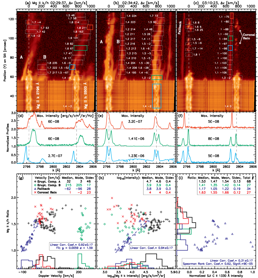
In the Doppler velocity distribution observed by IRIS, a striking feature is a two-component composition during the early phase of the eruption: a primary (A) bright and broad component being slightly blueshifted and/or mildly redshifted, and a secondary (B) highly redshifted, comparably faint and narrow component, as shown in 2. The two components, yet with different structures, are somewhat parallel to each other, separated by , with a similar trend of growing redshifts (up to ) with height. They can be identified in all bright lines, including the Mg II k 2796 Å and h 2803 Å, C II 1335 and 1336 Å, and Si IV 1403 Å lines. (Note that the C II 1335 Å component B almost overlaps with the 1336 Å component A.) One possibility consistent with the gap between the two components is that the erupting material is spatially distributed in a hollow, rather than solid, cone shape.
As time progresses, the two components gradually merge into a single component with decreasing line widths. At later times, the entire spectrum evolves from red- to blueshifts, while maintaining the same general slope with height as noted below (see 3, bottom). This evolution can be clearly seen from the wavelength– or velocity–time plot shown in 1(g), obtained by averaging the Mg II k 2796 Å spectra over the entire region above the chromospheric limb. We fitted the velocity–time positions of component B and later the merged single component with a smooth spline function, shown as the solid green curve, to characterize the temporal evolution. This curve exhibits an initially rapid and then gradual decline with time, similar to that of the POS velocity shown in 1(f). More interestingly, its crossing at zero Doppler velocity, i.e., the change from red- to blueshifts at 02:50 UT (marked by the vertical dotted line), coincides with the switch of sign for the POS velocity and the apexes of the ballistic POS trajectories shown in 1(e), indicating a transition from upward eruption to downward fallback of the material. This transition may also explain the onset of the faster drop of the Mg II k 2796 Å intensity at the same time (see 1(d), red line). The uncertainty of this temporal coincidence is estimated at minutes, bracketed by the zero-crossings of the two dotted lines in 1(g), which are the counterparts of the solid curve obtained near the bottom and top edges of the off-limb portion of the IRIS slit (at and , see 1(b)). This conservative error estimate can also account for the temporal spread of the turning points of the different POS trajectories shown in 1(e) and the uncertainty in the absolute Doppler velocity noted in Section 3.1.
We also note in 1(g) a persistent feature near zero Doppler shift, which is coronal rain in the foreground of the eruption. Because it is captured by the slit near the apexes of coronal loops where such cooling condensation is initially formed (e.g., Antolin et al., 2010; Liu et al., 2012; Fang et al., 2013), its small Doppler velocity, almost symmetrically distributed around zero, is expected and consistent with our selection of the reference wavelength described in Section 3.1.
We can estimate the 3D velocity vector using simultaneous POS and Doppler velocities. For example, during 02:30–02:45 UT, the two velocities (1(f), red crosses and green curve) are almost the same, indicating an angle of behind the POS. This is an upper limit, because the eruption component B has the highest redshift. A more accurate estimate can be obtained during the late phase when the velocity distribution is relatively simple. At 03:06:15 UT (see 3(h)), for instance, the fallback material exhibits blueshifts increasing almost linearly with decreasing heights. This is consistent with a similar trend of the POS velocity (white dashed line) obtained from the last parabolic trajectory in 1(e) covering this time. Specifically, the blueshift increases from to by 36% over the POS height range of () within the IRIS FOV. This percentage change is similar to the 33% increase of the POS velocity from at 03:03:32 UT to at 03:08:04 UT over the same height range. These two pairs of velocities give a consistent angle of between the velocity vector and POS. This provides additional support for our interpretation of the late-phase blueshift as evidence of material falling back, and implies that the fallback trajectory within this height range is oriented at a constant angle from the POS.
This parabolic space–time trajectory yields a downward POS acceleration of , which translates to a true 3D acceleration of , where is the solar surface gravitational constant. Note that Cut 1 (along which this trajectory is measured) is only from the POS projection of the radial direction and the angle of the velocity vector from the POS is close to the angle of the behind-the-limb location of the source flare. Therefore, this fallback path is likely close to the local vertical at the source111The exact 3D path of the fallback material is difficult to infer in this case, because of the inadequate cadence of STEREO-A and thus the unknown landing site behind the limb. and the effective gravitational acceleration along it is close to , greater than the measured . Such a less-than-free-fall acceleration, indicating cancellation of gravity by some upward force, is comparable to those (mostly measured in POS) of fallback material in chromospheric jets (e.g., Liu et al., 2009) and of coronal rain (e.g., Schrijver, 2001; Antolin & Rouppe van der Voort, 2012), but somewhat higher than those of downflow threads in quiescent prominences (e.g., van Ballegooijen & Cranmer, 2010; Chae, 2010; Liu et al., 2012; Low et al., 2012).
Another interesting feature of the fallback material is its narrow line width, which continues decreasing with time, as shown in 1(g). During the late phase after 03:10 UT (e.g., Figures 3(h) and 4(c)), its nonthermal line width is only on the order of , nearly 50% that of the foreground coronal rain at loop apexes. This indicates that such material falls along streamline trajectories with very little velocity scatter or nonthermal broadening. We speculate that this could be due to the lack of line broadening agents, such as small-scale Alfvén waves or turbulence, which likely accompany the impulsive eruption earlier but have diminished substantially ever since.
3.4. Helical Structure and Torsional Motions
Helical structures have been commonly seen in imaging or spectroscopic observations of solar eruptions, including CMEs (e.g., Kohl et al., 2006), prominence eruptions (Koleva et al., 2012), and jets or surges (Canfield et al., 1996; Liu et al., 2011). We found compelling new evidence in this event, with the combination of high-resolution SJIs and spectra offering critical clues to the 3D structure.
In the POS, AIA images show cork-screw shaped threads, especially early in the eruption when the morphology is relatively simple (e.g., Figures 1(a) and (b)). Their temporal evolution is manifested in the multiple sinusoidal tracks shown in 1(i), an IRIS C II 1330 Å SJI space–time plot obtained from Cut 2, perpendicular to the eruption axis. In contrast, during the late phase, e.g., after 03:00 UT, the falling material shows no longer sinusoidal, but essentially flat tracks. This suggests that the pre-stored magnetic helicity or twists have been transported into the heliosphere by the eruption and thus the falling material returns as streamline flows along untwisted field lines, similar to those in previously reported helical jets (e.g., Liu et al., 2009).
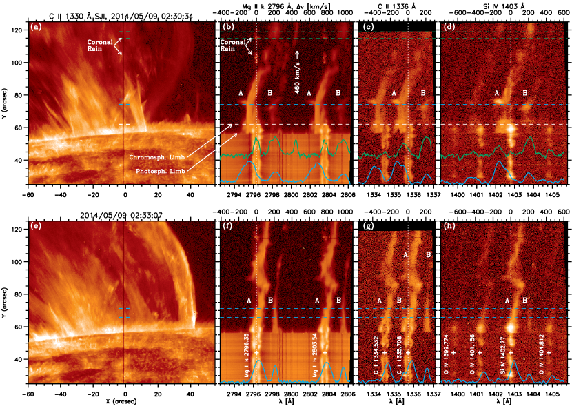
Doppler measurements by IRIS provide several clues for the interpretation of the above POS observations as torsional/rotational motions, rather than transverse oscillations. The IRIS slit is oriented at clockwise from the central axis of the eruption, allowing it to cover both sides of the axis, i.e., with its lower portion sampling the left-hand side and the upper portion sampling the right-hand side. We find that early in the eruption, the initial blueshifts of some individual features switch to redshifts with time as they travel upward along the slit (see 3(a)–(c) and Animation 2 for an example). Moreover, in single spectral snapshots, the primary (A) spectral component of the eruption at times show predominant blueshifts at lower heights that smoothly transition to redshifts at larger heights (e.g., 2(b) and 3(c)). The combination of these observations indicates a counter-clockwise rotation of the erupting material when viewed top-down. Note that sometimes both components A and B show no sign of blueshifts but only redshifts that generally grow with height. This can be explained by the fact that the eruption occurs behind the limb and large redshifts due to outward radial motions are expected and can reduce or even reverse the blueshifts caused by rotations.
We can further infer the handedness of the helices by combining POS and Doppler observations. Early in the event, SJIs show material threads progressing transversely from left to right. To be consistent with the above inferred counter-clockwise rotations with dominant blueshifts on the left, such threads must be located on the front side of the eruption, although the C II 1330 Å SJI emission is likely optically thin above the C II limb and thus we are seeing both the front and back sides. Noting that these threads are oriented from lower-right to upper-left, we conclude that they are left-handed helices. Their counter-clockwise rotations are thus consistent with relaxation or unwinding, rather than tightening, motions of the helices, which are expected for such an eruption.
We also found sinusoidal spectral variations along the slit and their progression toward greater heights with time, best seen during 02:31:12–02:32:19 UT (3(d)). This may be evidence of (multiple) small-scale ( across) helical sub-structures within the overall eruption, which are also evident in SJIs (e.g., see the unfolding feature near 02:45 UT in Animation 2).
3.5. Mg II k/h Line Ratio and Doppler Dimming
3.5.1 Mg II k/h Line Ratio
The Mg II k 2796 Å and h 2803 Å lines and their intensity ratio can provide useful plasma diagnostics (e.g., Leenaarts et al., 2013; Pereira et al., 2013). In general, this k/h ratio is expected to be 2 for optically thin, collisionally excited (thermal) emission. Previously reported values include 2 for an active-region prominence (Vial et al., 1979), 1.7 for a quiescent prominence (Vial, 1982a), and 1.33–1.35 for quiescent prominences recently observed by IRIS (Heinzel et al., 2014; Schmieder et al., 2014).
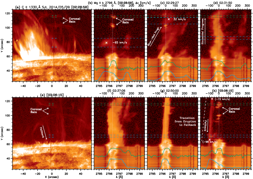
As shown in 4 (top), we identified various corresponding features in both the k and h lines, integrated their continuum-subtracted intensities, and obtained their ratios, which are labeled together with the line-centroid Doppler velocities. The mid row in 4 shows some sample spectra at selected positions. Unlike their on-disk or chromospheric counterparts, the off-limb Mg II k and h lines of both erupted material and coronal rain have no central reversal, similar to those in IRIS observed prominences (Heinzel et al., 2014; Schmieder et al., 2014), suggestive of a low pressure or thickness and optically-thin regime. Because the oscillator strength of the k line is twice that of the h line, the k line always has a larger integrated intensity. However, for the fallback material (4(f)), the k line has a comparably lower peak intensity.
We repeated this analysis for a total of 156 features selected from eight spectra through the course of this event. The resulting intensity ratio is plotted against the line-centroid Doppler velocity and k line intensity (4(g) and (h)), categorized for four types of features: the primary (A; black plus signs) and secondary (B; green diamonds) eruption components, fallback material (blue triangles), and coronal rain (red crosses). As a reference, the k/h ratios of the on-disk quiet Sun and chromosphere at the limb have medians and standard deviations of and , respectively. The coronal rain has the highest k/h ratio of , the lowest Doppler velocity nearly zero, and a moderate intensity. Eruption component A has a moderate k/h ratio of , a small Doppler velocity, and the highest intensity of . Eruption component B has a somewhat smaller ratio of , the highest Doppler velocity of redshifts, and a moderate intensity about 6 times smaller than that of component A. The fallback material has the lowest k/h ratio of , a moderate blueshift, and the lowest intensity.
The k/h ratios of the fallback material are particularly interesting, yet puzzling. During the late phase of the event, as progressively less material is present off-limb and as the intensity drops with time, one would expect the Mg II k and h emission to approach the optically-thin regime and thus a k/h ratio close to 2. However, the median ratio is surprisingly small, the lowest among all reported values for prominences and even less than those of the quiet-Sun disk () and chromosphere (). More interestingly, the k/h ratio is highly correlated with both the line-centroid Doppler velocity and the k line intensity , with linear correlation coefficients of and , respectively. A linear regression gives , leading to a ratio of unity at .
We also obtained C II 1330 Å SJI intensities averaged within the Y-direction ranges corresponding to those boxes defined in the spectra of the fallback material (e.g. 4(c)) and within an X-direction range of covering all the 8-step raster positions. They show a comparably weak but noticeable correlation with the k/h ratios. This is perhaps not surprising because of the similar temporal trends of the C II 1330 Å SJI and Mg II k line intensities, as shown in 1(d).
3.5.2 Doppler Dimming
Compared with the eruption components A and B with a complex morphology and dynamic evolution but lack of correlation in Figures 4(g) and (h), the fallback material has a relatively simple morphology in a relaxed, post-eruption state and a well-defined correlation between the Mg II k/h ratio and the Doppler velocity or line intensity. In this section, we thus focus on the fallback material to explore the underlying physics of such characteristics as the surprisingly low values of the k/h ratio. We note that the off-limb k and h lines have contributions from both radiative excitation by the solar surface radiation and local collisional (thermal) excitation. Their relative importance depends on the pressure (density and temperature) of the material and is estimated as follows.
We assume that the Mg II line emitting plasma is optically thin, an assumption valid only for thin, low-pressure prominence threads (see Table 2 of Heinzel et al., 2014). Then each plasma blob receives the full incident radiation and emits both scattered () and thermal () radiation. Regardless of the frequency redistribution process, is the product of the geometric dilution factor and the chromospheric intensity, for which we adopt the line-center intensity of from Heinzel et al. (2014). is the product of the photon destruction probability and the Planck function at the plasma temperature (see, e.g., Mihalas, 1978; Vial, 1982b). is proportional to the electron density and steadily increases with (so does ). We find that
-
1.
for a typical prominence density of (e.g., see Table 4 of Labrosse et al., 2010) and a low temperature of , the radiation term dominates over the collisional term by orders of magnitude, while
-
2.
an increase in density above and/or in temperature to would result in the collisional-term dominance.
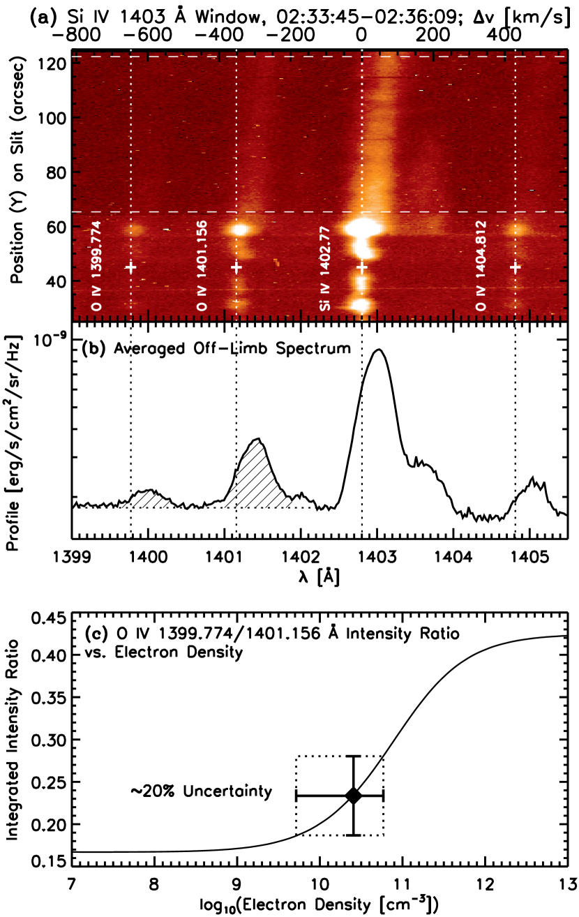
Determining the relative importance of and for the specific event under study requires the knowledge of the plasma density. To this end, we utilized the density sensitive O IV 1399.774/1401.156 Å line ratio. In order to increase the signal-to-noise ratio, we first obtained a spectrum (see 5(a)) by averaging two raster scans when these lines are relatively bright and overlaps due to Doppler shifts are relatively small. We then averaged all off-limb spectra to obtain the profile shown in 5(b), which then gives a continuum-subtracted, integrated O IV 1399.774/1401.156 Å intensity ratio of 0.234 for the primary (A) eruption component. According to the CHIANTI v7.1 database (Landi et al., 2013), this ratio translates to a predicted density of (see 5(c)). Its uncertainty originates mainly from line blending, which is estimated as follows: (i) We found that the O IV 1399.774 Å line is blended by the Fe II 1399.962 Å line at an upper-limit 6% level. To arrive at this order-of-magnitude estimate, we assumed that the Fe II and Mg II k lines are emitted by the same optically-thin plasma of a uniform differential emission measure (not necessarily true). We used the CHIANTI routine ch_synthetic.pro and assumed a constant pressure (corresponding to and for typical prominence conditions) to synthesize their respective contribution functions , which were then multiplied by the chromospheric abundance and the IRIS response function (from iris_get_response.pro) and integrated over a temperature range of – covering the peak to yield their line intensities, and . With the predicted ratio of and the observed Mg II k intensity, we estimated the Fe II 1399.962 Å intensity, which turned out to be 6% of the observed O IV 1399.774 Å intensity. (ii) We could not identify any S I 1401.514 Å line emission beyond the quiet-Sun disk and thus its blend to the O IV 1401.156 Å line is considered negligible. Nevertheless, we assumed a conservative 20% uncertainty for the line ratio, which gives a density range of – . This density pertains to the warm plasma at the O IV formation temperature of , which, in this case, is most likely located in the so-called prominence–corona transition region (PCTR; Parenti & Vial, 2014). In the cold prominence core at the Mg II k and h formation temperature of , the density could be times higher (assuming pressure equilibrium), but still smaller than the extreme density of required for the collisional-term dominance in the low temperature regime as mentioned above. Therefore, we conclude that the Mg II k and h emission of the erupted material is dominated by radiative excitation.

For radiatively excited emission from moving objects, there is a Doppler dimming effect in which the incident line emission from the solar surface is Doppler-shifted out of resonance. This effect has been extensively investigated for hydrogen and helium lines (e.g., Hyder & Lites, 1970; Heinzel & Rompolt, 1987; Gontikakis et al., 1997; Labrosse et al., 2007; Labrosse & McGlinchey, 2012) and recently modeled for the Mg II k and h lines (Heinzel et al., 2014). Note that the wings of the chromospheric k and h lines are somewhat different. Therefore, when a moving object resonantly absorbs the Doppler-shifted wings followed by de-excitation radiation, the emergent k/h ratio can depend on the Doppler velocity. This may potentially explain their observed correlation.
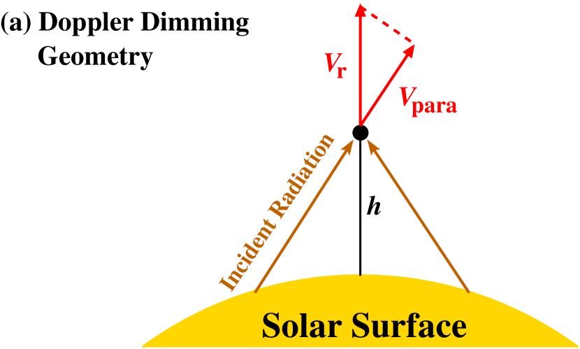
As a proof-of-concept exercise, we model the Mg II k/h ratio due to Doppler dimming as follows. Again, we assume that the erupted material is optically thin and ignore collisional excitation according to the above analysis. Thus the Mg II k and h emission is simply resonant scattering of the incident chromospheric radiation, with no radiative transfer taking place. We also assume that the solar surface is a sphere producing uniform radiation, for which we adopt an IRIS-observed quiet-Sun Mg II k and h spectrum, and ignore limb darkening or brightening. For an object at a height moving at a velocity in the radial direction, we calculate its incident radiation by integrating the Doppler-shifted radiation from the entire visible solar surface, as schematically shown in 6(a). This spatial average can alter the shape of the absorbed line profile, because the radial velocity has different parallel components projected along incident rays from different directions that determine the Doppler shifts. As an example, 6(b) and (c) show the average Mg II k and h profiles incident on an object moving at different velocities at a height of 100 Mm, which is near the lower limit of the height range of the IRIS-observed prominence material according to its behind-the-limb source location. At , the central reversals of both lines disappear. Because Mg is a heavy element, the thermal broadening is expected to be small and we assume a delta-function profile for the scattering agent (moving object). Thus the scattered emission is essentially the incident radiation at the line center (), as marked by the vertical dashed line. The ratio of the k and h intensity at this position, as shown in 6(d), would be equivalent to the observed line ratio. For a stationary object (), this k/h ratio is . For a moving object, the two lines are dimmed by different factors. At , for example, the k line center intensity is reduced by a factor of 0.10, while the h line by 0.14,leading to . Such dimming factors are on the same order of magnitude as those modeled for a moving prominence (Heinzel et al., 2014).
Repeating this for different height and velocity values, we obtained the dependence of the k/h ratio on these two quantities, as shown in 6(e). These curves have a butterfly shape and generally decrease with increasing or . There is a positive correlation between and near (0 for falling material), which qualitatively agrees with the observed correlation shown in 4(g). A blue-red asymmetry is present, with smaller k/h ratios for radially outward velocities (0), because of the asymmetry in the Mg II k and h wings. For lower heights, the butterfly curves have a broader top portion at values close to that at , because relatively more incident radiation originates from large angles away from the local radial direction at the object. Such radiation is less Doppler-shifted due to the smaller component of the assumed radial velocity projected along those rays.
Note that the eruption component B is about higher in Doppler velocity and a factor of 6 fainter in intensity than component A, and even fainter than the coronal rain. We suggest that Doppler dimming may contribute to its faintness, among other possible factors, such as a smaller emission measure. We also note that the gradual fading of the C II 1330 Å SJI intensity during the late phase (see 1(d) and online Animation 2) coincides with the increasing blueshifts and POS downflow velocities. We speculate that this fading may be due, at least in part, to Doppler dimming of the C II lines in a similar manner. In contrast, Doppler dimming has very little effect on the coronal rain detected near the loop apexes because of its small velocities.
4. Concluding Remarks
4.1. Summary
We have presented the first IRIS observations of a fast prominence eruption associated with a CME and an equivalent X1.6 flare on the far side of the Sun. We summarize our major findings as follows.
-
1.
The ejected material is detected in bright lines at chromospheric to transition-region temperatures (–). We find no obvious delay among lines at different temperatures, suggesting no detectable temperature changes (see Section 3.2).
-
2.
The prominence eruption has a maximum POS velocity of and redshift of , while the white-light CME has a maximum POS speed of (Section 3.3). These values are near the higher end of the velocity distribution reported for prominence eruptions. In contrast, the Doppler velocities of prominence material in the slower CME interior detected by SOHO/UVCS are on average only 10% of the POS speeds of the CME leading fronts seen by SOHO/LASCO (Giordano et al., 2013).
-
3.
The erupting material exhibits a cascade with time toward lower velocities, with a transition from upward ejection to downward fallback consistently manifested in both POS velocities and Doppler shifts (red to blue drift). During the fallback phase, at a given time, larger blueshifts are found at lower heights, consistent with the downward acceleration of the falling material; at a given height, the blueshift increases with time, consistent with the fact that material falling later returns from greater heights and is originally ejected at larger initial velocities earlier. A typical fallback trajectory has a less-than-free-fall, true 3D acceleration of , comparable to the values reported for falling ejecta and coronal rain. The fallback material exhibits a progressively narrower line width down to , indicative of streamline flows (see Section 3.3).
-
4.
There are two components of erupted material in Doppler velocity: a primary (A), bright component of comparably small Doppler shifts and a secondary (B), faint, highly redshifted component. The two components are separated by , suggestive of a hollow, rather than solid, cone shape, in which the material is distributed (Section 3.3). We also suggest that stronger Doppler dimming of component B can contribute to its relatively smaller intensity.
-
5.
The combination of a blue- to redshift transition with height along the slit and cork-screw shaped threads and sinusoidal transverse motions imaged in the POS indicates that the eruption involves a left-handed helical structure undergoing counter-clockwise (when viewed top-down) unwinding/relaxation motions (Section 3.4). Such a handedness originating from the southern hemisphere (AR 12051) is opposite to the dominant hemispheric rule of magnetic helicity for active regions (e.g., Pevtsov et al., 1995; Wang, 2013).
-
6.
We find a wide range of Mg II k/h line intensity ratios. The foreground coronal rain has the highest median ratio of , the eruption components A and B have intermediate values of and , respectively, while the fallback material has the lowest value of , the smallest ever reported. In addition, the k/h ratio of the fallback material is strongly correlated with the Doppler velocity and line intensity, with linear correlation coefficients at levels (Section 3.5.1).
-
7.
The low density of the prominence core inferred from the O IV 1399.774/1401.156 Å line ratio implies that the observed Mg II k and h emission is dominated by radiative (rather than collisional) excitation. Doppler dimming is thus expected to alter the emergent emission profile from moving objects. Our simple back-of-envelope calculation demonstrates that this effect may qualitatively explain the observed Mg II k/h ratios, especially the surprisingly low values found in the fallback material and their correlation with Doppler velocities (Section 3.5.2).
4.2. Discussion
New IRIS observations, such as these presented here, have opened a new diagnostic window to study CMEs/prominence eruptions. For example, once the thermodynamic parameters establish that the Mg II k and h emission is dominated by resonance scattering, the k/h ratio can provide, through the Doppler dimming factor, critical information about the radial velocity, height, and 3D geometry of the ejected material. Similar techniques have already been used for diagnosing solar wind and CME speeds in the outer corona (e.g., Kohl & Withbroe, 1982; Raymond & Ciaravella, 2004).
Another novel feature revealed by IRIS is that the erupting and returning material behind the limb both appear at spicule heights within the chromosphere in all bright lines at large Doppler shifts (see 2), alongside their corresponding rest-wavelength chromospheric emission at the foreground limb. These lines include the Mg II k and h and C II lines, which have central reversals in the chromospheric emission because of high opacity, but have no reversal in the Doppler-shifted, off-limb components indicating a largely optically-thin regime. In other words, IRIS “sees through” the chromosphere at the limb in certain Doppler-shifted lines of otherwise optically-thick chromospheric emission. This is equivalent to detecting emission at different wavelengths from different LOS depths of the on-disk atmosphere. This capability of simultaneously detecting behind-the-chromospheric-limb, Doppler-shifted material (which is usually not accessible to telescopes from the Earth view) and the foreground chromospheric material of the same temperature provides a unique, novel diagnostic potential yet to be explored, e.g., for partially occulted flares (e.g., Liu et al., 2008; Krucker & Lin, 2008).
The proof-of-concept estimate of Doppler dimming presented in Section 3.5.2 has its limitations with assumptions that may not be valid in the real situation. It explains some, but not all observed features including some high Mg II k/h ratio (1.6) of the highly redshifted eruption component B (4(g)). However, its promise demonstrated in the qualitative agreement with the observations warrants more detailed NLTE modeling with the inclusion of, e.g., a 2D or 3D geometry, velocity vectors for Doppler dimming effects, and, as in Heinzel et al. (2014), the presence of a prominence–corona transition region, which we plan to pursue in the future. We also plan to use multi-instrument observations to infer the detailed 3D geometry and velocity vector as well as the escaping and returning mass fluxes.
References
- Antolin & Rouppe van der Voort (2012) Antolin, P. & Rouppe van der Voort, L. 2012, ApJ, 745, 152
- Antolin et al. (2010) Antolin, P., Shibata, K., & Vissers, G. 2010, ApJ, 716, 154
- Avrett et al. (2013) Avrett, E., Landi, E., & McKillop, S. 2013, ApJ, 779, 155
- Canfield et al. (1996) Canfield, R. C., Reardon, K. P., Leka, K. D., Shibata, K., Yokoyama, T., & Shimojo, M. 1996, ApJ, 464, 1016
- Chae (2010) Chae, J. 2010, ApJ, 714, 618
- Chen (2011) Chen, P. F. 2011, Liv. Rev. Solar Phys., 8, 1
- Ciaravella et al. (1997) Ciaravella, A., Raymond, J. C., Fineschi, S., Romoli, M., Benna, C., Gardner, L., Giordano, S., Michels, J., O’Neal, R., Antonucci, E., Kohl, J., & Noci, G. 1997, ApJ, 491, L59
- De Pontieu et al. (2014) De Pontieu, B., Title, A. M., Lemen, J. R., et al.. 2014, Sol. Phys., 289, 2733
- Fang et al. (2013) Fang, X., Xia, C., & Keppens, R. 2013, ApJ, 771, L29
- Fontenla & Poland (1989) Fontenla, J. M. & Poland, A. I. 1989, Sol. Phys., 123, 143
- Giordano et al. (2013) Giordano, S., Ciaravella, A., Raymond, J. C., Ko, Y.-K., & Suleiman, R. 2013, J. Geophys. Res. (Space Physics), 118, 967
- Gontikakis et al. (1997) Gontikakis, C., Vial, J.-C., & Gouttebroze, P. 1997, A&A, 325, 803
- Harra et al. (2007) Harra, L. K., Hara, H., Imada, S., Young, P. R., Williams, D. R., Sterling, A. C., Korendyke, C., & Attrill, G. D. R. 2007, PASJ, 59, 801
- Heinzel & Rompolt (1987) Heinzel, P. & Rompolt, B. 1987, Sol. Phys., 110, 171
- Heinzel et al. (2014) Heinzel, P., Vial, J.-C., & Anzer, U. 2014, A&A, 564, A132
- Hundhausen et al. (1984) Hundhausen, A. J., Sawyer, C. B., House, L., Illing, R. M. E., & Wagner, W. J. 1984, J. Geophys. Res., 89, 2639
- Hyder & Lites (1970) Hyder, C. L. & Lites, B. W. 1970, Sol. Phys., 14, 147
- Jin et al. (2009) Jin, M., Ding, M. D., Chen, P. F., Fang, C., & Imada, S. 2009, ApJ, 702, 27
- Kohl et al. (2006) Kohl, J. L., Noci, G., Cranmer, S. R., & Raymond, J. C. 2006, A&A Rev., 13, 31
- Kohl & Parkinson (1976) Kohl, J. L. & Parkinson, W. H. 1976, ApJ, 205, 599
- Kohl & Withbroe (1982) Kohl, J. L. & Withbroe, G. L. 1982, ApJ, 256, 263
- Koleva et al. (2012) Koleva, K., Madjarska, M. S., Duchlev, P., Schrijver, C. J., Vial, J.-C., Buchlin, E., & Dechev, M. 2012, A&A, 540, A127
- Krucker & Lin (2008) Krucker, S. & Lin, R. P. 2008, ApJ, 673, 1181
- Labrosse et al. (2007) Labrosse, N., Gouttebroze, P., & Vial, J.-C. 2007, A&A, 463, 1171
- Labrosse et al. (2010) Labrosse, N., Heinzel, P., Vial, J.-C., Kucera, T., Parenti, S., Gunár, S., Schmieder, B., & Kilper, G. 2010, Space Sci. Rev., 151, 243
- Labrosse & McGlinchey (2012) Labrosse, N. & McGlinchey, K. 2012, A&A, 537, A100
- Landi et al. (2013) Landi, E., Young, P. R., Dere, K. P., Del Zanna, G., & Mason, H. E. 2013, ApJ, 763, 86
- Leenaarts et al. (2013) Leenaarts, J., Pereira, T. M. D., Carlsson, M., Uitenbroek, H., & De Pontieu, B. 2013, ApJ, 772, 89
- Liu et al. (2012) Liu, W., Berger, T. E., & Low, B. C. 2012, ApJ, 745, L21
- Liu et al. (2009) Liu, W., Berger, T. E., Title, A. M., & Tarbell, T. D. 2009, ApJ, 707, L37
- Liu et al. (2011) Liu, W., Berger, T. E., Title, A. M., Tarbell, T. D., & Low, B. C. 2011, ApJ, 728, 103
- Liu & Ofman (2014) Liu, W. & Ofman, L. 2014, Sol. Phys., 289, 3233
- Liu et al. (2008) Liu, W., Petrosian, V., Dennis, B. R., & Jiang, Y. W. 2008, ApJ, 676, 704
- Low et al. (2012) Low, B. C., Liu, W., Berger, T., & Casini, R. 2012, ApJ, 757, 21
- Mackay et al. (2010) Mackay, D. H., Karpen, J. T., Ballester, J. L., Schmieder, B., & Aulanier, G. 2010, Space Sci. Rev., 151, 333
- Martin (1998) Martin, S. F. 1998, Sol. Phys., 182, 107
- Mihalas (1978) Mihalas, D. 1978, Stellar Atmospheres, 2nd edition (San Francisco, W. H. Freeman and Co., 650 p.)
- Nitta et al. (2013) Nitta, N. V., Aschwanden, M. J., Boerner, P. F., Freeland, S. L., Lemen, J. R., & Wuelser, J.-P. 2013, Sol. Phys., 288, 241
- Parenti (2014) Parenti, S. 2014, Living Reviews in Solar Physics, 11, 1
- Parenti & Vial (2014) Parenti, S. & Vial, J.-C. 2014, in IAU Symposium, Vol. 300, Nature of Prominences and Their Role in Space Weather, ed. B. Schmieder, J.-M. Malherbe, & S. T. Wu, 69–78
- Penn (2000) Penn, M. J. 2000, Sol. Phys., 197, 313
- Pereira et al. (2013) Pereira, T. M. D., Leenaarts, J., De Pontieu, B., Carlsson, M., & Uitenbroek, H. 2013, ApJ, 778, 143
- Pevtsov et al. (1995) Pevtsov, A. A., Canfield, R. C., & Metcalf, T. R. 1995, ApJ, 440, L109
- Raymond & Ciaravella (2004) Raymond, J. C. & Ciaravella, A. 2004, ApJ, 606, L159
- Raymond et al. (2003) Raymond, J. C., Ciaravella, A., Dobrzycka, D., Strachan, L., Ko, Y.-K., Uzzo, M., & Raouafi, N.-E. 2003, ApJ, 597, 1106
- Schmahl & Hildner (1977) Schmahl, E. & Hildner, E. 1977, Sol. Phys., 55, 473
- Schmieder et al. (2014) Schmieder, B., Tian, H., Kucera, T., López Ariste, A., Mein, N., Mein, P., Dalmasse, K., & Golub, L. 2014, A&A, 569, A85
- Schrijver (2001) Schrijver, C. J. 2001, Sol. Phys., 198, 325
- Schwenn (1996) Schwenn, R. 1996, Ap&SS, 243, 187
- St. Cyr et al. (2000) St. Cyr, O. C., Plunkett, S. P., Michels, D. J., Paswaters, S. E., Koomen, M. J., Simnett, G. M., Thompson, B. J., Gurman, J. B., Schwenn, R., Webb, D. F., Hildner, E., & Lamy, P. L. 2000, J. Geophys. Res., 105, 18169
- Tandberg-Hanssen (1995) Tandberg-Hanssen, E. 1995, The nature of solar prominences (Dordrecht; Boston: Kluwer)
- Tian et al. (2012) Tian, H., McIntosh, S. W., Xia, L., He, J., & Wang, X. 2012, ApJ, 748, 106
- Tian et al. (2013) Tian, H., Tomczyk, S., McIntosh, S. W., Bethge, C., de Toma, G., & Gibson, S. 2013, Sol. Phys., 288, 637
- van Ballegooijen & Cranmer (2010) van Ballegooijen, A. A. & Cranmer, S. R. 2010, ApJ, 711, 164
- Vial (1982a) Vial, J. C. 1982a, ApJ, 253, 330
- Vial (1982b) —. 1982b, ApJ, 254, 780
- Vial et al. (1979) Vial, J. C., Gouttebroze, P., Artzner, G., & Lemaire, P. 1979, Sol. Phys., 61, 39
- Wang (2013) Wang, Y.-M. 2013, ApJ, 775, L46
- Webb & Howard (2012) Webb, D. F. & Howard, T. A. 2012, Liv. Rev. Solar Phys., 9, 3
- Widing et al. (1986) Widing, K. G., Feldman, U., & Bhatia, A. K. 1986, ApJ, 308, 982
- Wiik et al. (1997) Wiik, J. E., Schmieder, B., Kucera, T., Poland, A., Brekke, P., & Simnett, G. 1997, Sol. Phys., 175, 411