Superconductivity in the elements, alloys and simple compounds

Abstract

We give a brief review of superconductivity at ambient pressure in elements, alloys, and simple three-dimensional compounds. Historically these were the first superconducting materials studied, and based on the experimental knowledge gained from them the BCS theory of superconductivity was developed in 1957. Extended to include the effect of phonon retardation, the theory is believed to describe the subset of superconducting materials known as ‘conventional superconductors’, where superconductivity is caused by the electron-phonon interaction. These include the elements, alloys and simple compounds discussed in this article and several other classes of materials discussed in other articles in this Special Issue.

I introduction

Superconductivity was discovered by Kamerlingh Onnes in 1911 in $Hg$ hg , and in $Pb$ and $Sn$ within the next two years pbsn . By 1932, $Tl$, $In$, $Ga$, $Ta$, $Ti$, $Th$ and $Nb$ had also been found to be superconductors meissner . By 1935, 15 superconducting elements were known smith , 19 by 1946 justi , 22 by 1954 eisenstein . Today, 31 elements are known to be superconducting at ambient pressure buzea ; liexp , many more at high pressures hamlinshimizu . Critical temperatures of the elements at ambient pressure range from $0.0003$ K for $Rh$ to $9.25$ K for $Nb$.

Table 1: Some superconducting alloys and compounds known in 1935 smith .

Material	$T_{c}$	Material	$T_{c}$
$Bi_{6}Tl_{3}$	$6.5K$	$TiN$	$1.4K$
$Sb_{2}Tl_{7}$	$5.5$	$TiC$	$1.1$
$Na_{2}Pb_{5}$	$7.2$	$TaC$	$9.2$
$Hg_{5}Tl_{7}$	$3.8$	$NbC$	$10.1$
$Au_{2}Bi$	$1.84$	$ZrB$	$2.82$
$CuS$	$1.6$	$TaSi$	$4.2$
$VN$	$1.3$	$PbS$	$4.1$
$WC$	$2.8$	$Pb-As$ alloy	$8.4$
$W_{2}C$	$2.05$	$Pb-Sn-Bi$	$8.5$
$MoC$	$7.7$	$Pb-As-Bi$	$9.0$
$Mo_{2}C$	$2.4$	$Pb-Bi-Sb$	$8.9$

Shortly after superconductivity in $Hg$ was discovered in 1911, alloys of $HgAu$, $HgCd$ $HgSn$ and $PbSn$ were also measured and found to be superconducting pbsn . By 1932 meissner , a large number of binary alloys and compounds had been found to be superconducting including $Au_{2}Bi$, with both elements non-superconducting aubi . It was also found that when alloying a non-superconducting metal with a superconducting one $T_{c}$ may be increased. Superconducting binary compounds with one of the elements nonmetallic were found meissner , e.g. $NbC$, with $T_{c}=10.1$ K, a non-superconducting metal with an insulator, $CuS$, $T_{c}=1.6$ K cus and many other binary compounds, particularly sulfides, nitrides and carbides meissner . These early findings demonstrated that superconductivity is a property of the solid, not of the elements forming the solid. Table 1 gives examples of superconducting compounds discussed in a 1935 review smith .

These experimental results indicated that the energy scale associated with superconductivity was of order $k_{B}T_{c}\sim 10^{-4}$ eV. On the other hand, it was generally believed at the time that superconductivity originated from the electron-electron interaction neglected in Bloch’s theory of electrons in single-particle energy bands. Thus a major puzzle was to understand how an interaction many orders of magnitude larger could give rise to the low $T_{c}$’s measured experimentally.

Table 2: Critical temperature and Debye temperature of superconducting elements known in 1946 justi .

Metal	$T_{c}$	$\theta_{D}$
$Nb$	$9.22$	$184$
$Pb$	$7.26$	$86$
$La$	$4.71$	$?$
$Ta$	$4.38$	$246$
$V$	$4.3$	$69$
$Hg$	$4.12$	$69$
$Sn$	$3.69$	$180$
$In$	$3.37$	$150$
$Tl$	$2.38$	$100$
$Ti$	$1.81$	$400$
$Th$	$1.32$	$200$
$U$	$1.25$	$141$
$Al$	$1.14$	$305$
$Ga$	$1.07$	$125$
$Re$	$0.95$	$283$
$Zn$	$0.79$	$230$
$Zr$	$0.70$	$288$
$Cd$	$0.54$	$158$
$Hf$	$0.35$	$?$

In Table II we list the 19 superconducting elements known by the year 1946, from a paper by E. Justi justi . The table also gives the Debye temperatures as given in that paper. It is interesting that Justi discusses in this paper the possible effect of the ionic mass and Debye temperature on the critical temperature. He reasoned that because lattice vibrations give rise to Ohmic resistance, one might expect a connection between Debye temperature and superconducting $T_{c}$. However, from the data in Table II he concluded that there is no relation between $\theta_{D}$ and $T_{c}$ justi . In addition he discussed an experiment performed in 1941 justi2 attempting to detect any difference in the critical temperature of the two $Pb$ isotopes ${}^{206}Pb$ and ${}^{208}Pb$ and finding identical results to an accuracy $1/1000$. From these observations he concluded in 1946 that the ionic mass has no influence on superconductivity.

The possible relation between Debye temperature and superconducting critical temperature was also examined by de Launay and Dolecek in 1947 isotope2 . In their paper “Superconductivity and the Debye characteristic temperature” they plotted the critical temperature versus Debye temperature. From this they concluded that electronegative elements have $T_{c}$’s well above the $T_{c}$’s of electropositive elements of comparable Debye temperatures, except in the range of lowest Debye temperatures where they converge. Combining these data with the atomic volumes they predicted that, at atmospheric pressure, Scandium and Yttrium should not be superconducting (correct) and that Ce, Pr and Nd should be superconducting (incorrect).

Table 3: Critical temperature, Debye temperature, atomic mass, measured and calculated isotope exponents of superconducting elements. Measured values are taken from a table in Ref. [isotope, ] and theoretical values are taken from a table in Ref. [garland63, ].

Metal	$T_{c}$	$\theta_{D}$	M	$\alpha$	$\alpha_{theory}$
$Nb$	$9.25$	$275$	93
$Tc$	$8.2$	$450$	99
$Pb$	$7.2$	$105$	207	0.48	0.47
$La$	$6$	$142$	139
$V$	$5.4$	$380$	51		0.15
$Ta$	$4.4$	$240$	181		0.35
$Hg$	$4.15$	$72$	201	0.5	0.465
$Sn$	$3.7$	$200$	119	0.46	0.44
$In$	$3.4$	$108$	115
$Tl$	$2.4$	$78.5$	204	0.5	0.445
$Re$	$1.7$	$430$	186	0.38	0.3
$Th$	$1.4$	$163$	232
$Pa$	$1.4$	$?$	231
$U$	$1.3$	$207$	238	-2
$Al$	$1.18$	$428$	27		0.345
$Ga$	$1.08$	$320$	70
$Am$	$1$	$154$	243
$Mo$	$0.92$	$450$	96	0.37	0.35
$Zn$	$0.85$	$327$	65	0.3
$Os$	$0.7$	$500$	190	0.21	0.1
$Zr$	$0.6$	$291$	91	0	0.35
$Cd$	$0.52$	$209$	112	0.5	0.365
$Ru$	$0.5$	$600$	101	0	0.0
$Ti$	$0.5$	$420$	48		0.2
$Hf$	$0.38$	$252$	176		0.3
$Ir$	$0.1$	$420$	192		-0.2
$Lu$	$0.1$	$210$	139
$Be$	$1440$	$1440$	9
$W$	$0.01$	$400$	184
$Li$	$0.0004$	$344$	7
$Rh$	$0.0003$	$480$	103

In view of these investigations it is remarkable that just three years later in 1950 Herbert Fröhlich proposed frohlich that superconducting critical temperatures should be proportional to $M^{-\alpha}$, with $M$ the ionic mass and $\alpha=0.5$ the isotope exponent. This was done without knowledge view1 ; view2 ; view3 of the isotope effect experiments maxwell ; serin being conducted at the same time that measured an isotope exponent $\alpha\sim 0.5$ in $Hg$ and shortly thereafter in $Pb$ pb , $Sn$ and $Tl$ sn . Table III lists the isotope exponents of these and several other elements measured since then isotope ; garland63 .

After the experimental findings of an isotope effect, the focus of theoretical efforts to understand the origin of the interaction leading to superconductivity shifted from the electron-electron interaction to the electron phonon interaction. In 1957 BCS developed their theory based on an effective instantaneous attractive interaction between electrons mediated by phonons bcs , that also predicts $\alpha=0.5$. BCS theory, extended to take into account the fact that the effective interaction between electrons mediated by phonons is not instantaneous but retarded, is believed to describe the superconductivity of all elements at ambient pressure, and of thousands of superconducting compounds. The tabulation by Roberts (1976) roberts lists several tens of thousands of superconducting alloys and compounds, almost all with critical temperatures below $20K$, believed to be described by BCS theory.

II Response to a Magnetic Field: Phenomenology

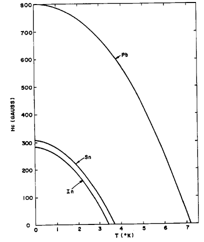
Figure 1: (a) Upper panel shows the $H_{c}$ vs temperature curves for three elemental type-I superconductors. (b) Lower panel shows the upper critical field, $H_{c2}$ for several superconducting compounds, belonging to various families. Note the huge difference in critical magnetic field strengths between type-I (a) and type-II (b) superconductors. Figure in (a) adapted from Ref. [cody73, ] and figure in (b) used from Tables of Physical & Chemical Constants (16th edition 1995). 2.1.4 Hygrometry. Kaye & Laby Online. Version 1.0 (2005).

Much of the focus for superconducting materials is on increasing $T_{c}$. This is of course important for applications, but as Geballe et al. geballe emphasize, it is also a primary measure of our understanding of the mechanism for superconductivity. In contrast the response of a material to an applied magnetic field is more generic, in the sense that a microscopic theory is usually not required to understand this response. In fact the Ginzburg-Landau theory ginzburg50 often suffices to provide a detailed description of the magnetic state, whether the material is type-I or type-II. In a type-I superconductor the magnetic response is perfect diamagnetism, with the magnetic field completely expelled provided the field strength is less than a critical value, $H_{c}$. At this field value the material reverts to the normal state. In a type-II superconductor, the material exhibits perfect diamagnetism up to a critical field $H_{c1}$; with increasing applied field, flux begins to penetrate the material in the form of vortices. This continues to occur up to an upper critical field, $H_{c2}$, after which they become normal remark0 .

Since $H_{c2}>>H_{c}$ (by several orders of magnitude), type-II superconductors are most useful in applications that have a magnetic field present. Whether a material is a type-I or a type-II superconductor depends on the so-called Ginzburg-Landau parameter, $\kappa\equiv\lambda/\xi$, where $\lambda$ is the penetration depth and $\xi$ is the superconducting coherence length. Since the coherence length can decrease with a decreased scattering length, then a type-I superconductor can be made into a type-II superconductor through disorder. There are approximately 30 pure elements that superconduct at atmospheric pressure; three of these, $Nb$, $V$, and $Tc$ are type-II while the rest are type-I. Essentially all compounds are type-II. In Fig. 1 we show some experimental data for the critical fields of (a) a few type-I elemental superconductors, and (b) a few type-II superconducting compounds. Note that while the temperature scale in (b) is about a factor of 3 higher than in (a), the magnetic field strengths in (b) about 1000 times higher than in (a).

III BCS theory and its extensions (Eliashberg)

The papers in this Special Issue each deal with a particular family of superconductor. By design they focus on the materials and experimental properties, with limited theoretical discussion. As Bernd Matthias said it in the famous ‘Science’ debate with Philip Anderson anderson64 , we wanted to focus on ‘The Facts’. Nonetheless, as the reader will see from the various contributions in this Issue, it is difficult to examine material properties without an underlying theoretical framework. For example, the McMillan equation mcmillan68 comes up in a number of places as a means to understand trends in superconducting $T_{c}$. We therefore felt it would be useful to provide here a sketch of the ‘conventional’ theory of superconductivity.

The zero temperature BCS theory bcs consists of a variational wave function, motivated by a collection of Cooper pairs cooper56 . Using this wave function, and a mean field simplification at finite temperature, one arrives at the simplest form for the superconducting transition temperature, given by

$$T_{c}=1.13\theta_{D}e^{-1/[g(\epsilon_{F})V]}$$ (1)

where $g(\epsilon_{F})$ is the density of states at the Fermi energy and $V$ is the effective electron-electron attraction within a range $\hbar\omega_{D}\equiv k_{B}\theta_{D}$ of the Fermi energy. One should take special note that BCS theory is a pairing theory, and in principle, has nothing to say about pairing mechanism. Here, following BCS bcs , a phonon mechanism is implied by the use of a cut off energy, $k_{B}\theta_{D}$. Many extensions of BCS theory are possible beyond this simple model, spanning minor considerations like a non-constant density of states near the Fermi level, to more serious modifications like inhomogeneities (leading to the Bogoliubov-de Gennes (BdG) equations degennes66 ), or an order parameter with nodes, or significant retardation effects (leading to Eliashberg theory eliashberg60 ). In discussing superconductivity amongst the elements, Eliashberg theory is required for a quantitative understanding of many of the superconducting properties, so we will expand in this direction below.

BCS theory alone allows us to understand a number of simple but important properties, which we now discuss before moving on to Eliashberg theory. First, as already mentioned, superconducting $T_{c}$ will have an isotope effect, and since $T_{c}\propto\theta_{D}$, then $T_{c}\propto M^{-\alpha}$ with $\alpha=0.5$. As mentioned already by Geballe et al. geballe , even in the absence of theoretical motivation, Kamerlingh Onnes and Tuyn onnes23 looked (unsuccessfully) for an isotope effect in Pb in 1923, as did Justi justi2 18 years later; then one was found in 1950 in Hg maxwell ; serin . BCS theory predicts an energy gap in the single particle density of states; this was confirmed by tunneling measurements a number of years later giaever60 . Finally, one of the non-intuitive confirmations of BCS theory is the observation of the so-called Hebel-Slichter coherence peak in the NMR relaxation rate of Aluminum hebel57 ; redfield59 , where the relaxation rate rises initially as the temperature is lowered below $T_{c}$, before becoming suppressed due to the opening of a gap.

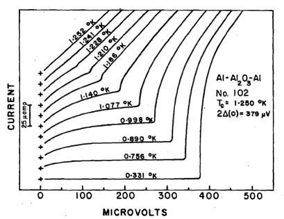
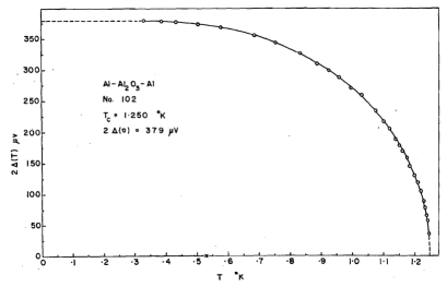
Figure 2: (a) IV characteristics for Al-I-Al junctions, and (b) the resulting normalized superconducting gap as a function of reduced temperature (points) compared with BCS theory (curve). The agreement is very good. From Ref. [black68, ].

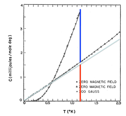
Figure 3: Specific heat measurements in both the normal and superconducting states for Al (from Ref. [phillips59, ]). Normal state results are achieved by the application of a magnetic field of 300 Gauss. The lightly shaded line and the two vertical lines have been added to indicate the normal state electronic specific heat ($\gamma T$) (grey) and the normal state electronic contribution at $T_{c}$ ($\gamma T_{c}$) (red) and additional jump at $T_{c}$ as predicted by BCS theory ($\Delta C_{es}=1.43\gamma T_{c}$) (blue), respectively. The data in the superconducting state is in very good agreement (slightly lower) than the BCS weak coupling prediction. Adapted from Ref. [phillips59, ].

Examples of some experiments with excellent agreement with BCS theory are the tunneling measurements for Al-I-Al junctions (see Fig. 2) and specific heat measurements on Al (see Fig. 3). There are many others in the literature parks69 . It is clear from these examples that Aluminum is the ‘poster child’ for BCS weak coupling theory. Nonetheless, even amongst the elemental superconductors there exist so-called ‘bad actors’ whose properties clearly do not conform quantitatively to BCS theory. Eliashberg theory was explored in part because of these discrepancies, and the ‘poster child’ for Eliashberg theory is Lead. Many reviews scalapino69 ; mcmillan69 ; allen82 ; rainer86 ; carbotte90 ; marsiglio08 , have been written on this subject, so here we will highlight some of the experimental manifestations. Note that Eliashberg theory is sometimes called the strong coupling version of BCS theory; this is somewhat of a misnomer, as both are developments with Fermi Liquid Theory as a starting point, and the term ‘strong coupling’ is generally reserved for situations in which kinetic energy (and therefore Fermi Liquid ideas) is initially ignored. It is more accurate to refer to Eliashberg theory as an extension of BCS theory with retardation effects properly taken into account remark1 .

The order parameter in Eliashberg theory becomes frequency dependent and complex. Both of these complications result from retardation effects. One of the immediate manifestations of this theory is a series of non-universal results for various properties that are universal within BCS theory. But even the theory for $T_{c}$ becomes more complicated, as epitomized, for example, by the McMillan equation mcmillan68 ; allen75 for $T_{c}$:

$$T_{c}={\hbar\omega_{\rm\ell n}\over 1.2k_{B}}\exp{\biggl{(}{-1.04(1+\lambda)\over\lambda-\mu^{\ast}(1+0.62\lambda)}\biggr{)}}$$ (2)

where $\omega_{\rm\ell n}$ is used as an average phonon frequency, and it and $\lambda$ are defined by

$$\omega_{\ln}\equiv\exp{\left[{2\over\lambda}\int_{0}^{\infty}d\nu\,\ln{(\nu)}{\alpha^{2}(\nu)F(\nu)\over\nu}\right]}$$ (3)

and

$$\lambda\equiv 2\int_{0}^{\infty}d\nu\,{\alpha^{2}(\nu)F(\nu)\over\nu}.$$ (4)

Both of these parameters are related to moments of the so-called Eliashberg function, $\alpha^{2}(\nu)F(\nu)$; this function describes the modes of excitations (in this case phonons) through which electrons effectively attract one another. They do this by emitting virtual phonons, in analogy to the photon exchange for the ordinary Coulomb interaction. But phonon propagation is several orders of magnitude slower than photon propagation, so properly accounting for this time delay means one electron attracts the other not to itself, but to where it used to be. This ‘dynamics’ also accounts for the smallness of the direct Coulomb interaction between two electrons, depicted by $\mu^{\ast}$. This repulsion would be overwhelmingly large, except that the two electrons are not in the same place at the same time, when they best take advantage of the virtual phonon exchange. This diminishing effect of the direct Coulomb potential is crucial for phonon-mediated superconductivity, and is known as the pseudo potential effect bogoliubov58 ; morel62 , with an expression given by

$$\mu^{\ast}={\mu\over 1+\mu\ln{({\epsilon_{F}\over\hbar\omega_{D}})}},$$ (5)

with $\epsilon_{F}$ the Fermi energy and $\mu=g(\epsilon_{F})U$ the dimensionless ‘bare’ Coulomb interaction. Typically $\epsilon_{F}>>\hbar\omega_{D}$, and so $\mu^{\ast}<<\mu$, with a limiting value of $1/\ln{(\epsilon_{F}/(\hbar\omega_{D})}$. This scaling of the Coulomb repulsion is also responsible for making calculations more tractable, as frequencies out to several (say, 6) times the phonon energy scale are required (about 60 meV for Lead), compared with several times the electronic bandwidth (about 2 orders of magnitude higher). A simple model illustrating this can be found in Ref. [marsiglio92, ].

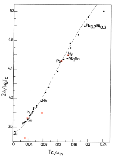
Figure 4: The gap ratio $2\Delta_{0}/(k_{B}T_{c})$ as a function of $T_{c}/\omega_{\rm\ell n}$. The black circles indicate theoretical calculations, with some of the elements and a couple of binary alloys indicated. The unmarked circles refer mostly to various binary alloys mitrovic84 . These calculations use an electron-phonon spectral function $\alpha(\nu)^{2}F(\nu)$ and value of $\mu^{\ast}$ extracted from tunneling experiments, or, in some cases taken from calculations carbotte67 ; carbotte68 . Selected experimental values are indicated with red squares. Note the excellent agreement of theory with experiment in the case of Sn, Pb and Hg, with more deviation in the case of Vanadium and Niobioum. Sources are available in Ref. [mitrovic84, ]. Figure is taken and then adapted from Ref. [mitrovic84, ].

Damping effects are essentially left out of simplifications like the McMillan equation, except for the presence of the mass enhancement factor, $1+\lambda$, in the numerator of the exponential. This tells us that the electron does become heavier as a result of the electron-phonon interaction, and $m^{\ast}/m\approx 1+\lambda$ is essentially the weak coupling remnant of the polaronic mass enhancement.

Full solutions of the Eliashberg equations display non-universality of various dimensionless quantities as a function of retardation effects. Mitrović et al. mitrovic84 identified a dimensionless parameter that grows from zero with increasing retardation effects; this is $T_{c}/\omega_{\rm\ell n}$. As this parameter tends to zero, various superconducting properties tend to their BCS limit. An example is the gap ratio, $2\Delta_{0}/(k_{B}T_{c})$, and a plot of this property vs. $T_{c}/\omega_{\rm\ell n}$ is shown in Fig. 4, along with some experimental data. Mitrović et al. derived an approximate expression,

$${2\Delta_{0}\over(k_{B}T_{c})}=3.53\biggl{[}1+12.5\bigl{(}{T_{c}\over\omega_{\ln}}\bigr{)}^{2}\ln{({\omega_{\ln}\over 2T_{c}})}\biggr{]},$$ (6)

which is also plotted as a dashed line. This simple expression clearly captures the essence of the theoretical results; note that some of the experimental values are in close agreement with the theoretical ones, while others remain closer to the universal BCS value.

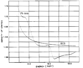
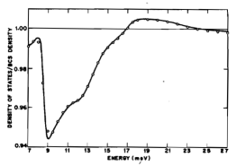
Figure 5: (a) The density of states for a Pb superconductor, obtained from conductance measurements of a Pb-I-Pb tunnel junction mcmillan69 . The BCS theory expectation value is shown for comparison. In (b) the extracted $\alpha^{2}(\nu)F(\nu)$ is shown (referred to as $\alpha^{2}(\nu)g(\nu)$ in the figure; this is obtained by demanding that the theory reproduce exactly the observed modulations with frequency. Also superimposed is the phonon density of states (denoted $g(\nu)$ in the figure) as measured through neutron scattering roy70 ; the rough agreement makes it clear that the excitations responsible for the modulations are phonons. Note that a number of consistency checks all prove positive. For example, the spectral function turns out to be positive definite (as it must), the required value of $\mu^{\ast}$ is positive (indicating a competing repulsion and not an additional attractive mechanism) and finally, in part (c) a comparison of the theory (curve) and experiment (points) in the ‘multiple-phonon-emission’ region is shown to illustrate the predictive power of the Eliashberg theory mcmillan69 . Figures in (a) and (c) are from Ref. [mcmillan69, ] and the figure in (b) is from Ref. [roy70, ].

The strongest evidence for the applicability of Eliashberg theory to elemental superconductors comes from tunneling measurements. Very early on observed modulations as a function of frequency in the measured current-voltage characteristics, especially in Lead, were suspected of being due to the electron-phonon interaction. Model calculations rowell63 ; schrieffer63 confirmed that Eliashberg theory could explain these modulations, and a short while later McMillan and Rowell mcmillan65 used Eliashberg theory to invert the tunneling data and extract $\alpha^{2}(\nu)F(\nu)$ and $\mu^{\ast}$. The latter was fit to a measurement of the tunneling gap edge, for example. An example of the data and the spectrum extracted from this data are shown in Fig. 5, and explained in that figure caption. Further explanation is available in Ref. [mcmillan69, ].

These have been interpreted as being very strong indications of the validity of Eliashberg Theory for elemental superconductors. Probably the ‘Achilles heel’ for which at the very least further understanding is required is the significant reduction of the direct Coulomb repulsion, manifested in the single number, $\mu^{\ast}$.

IV Isotope effect

The simplest BCS prediction for the isotope effect, using Eq. 1 is that the isotope coefficient, $\alpha=0.5$. Use of Eliashberg theory does not alter this result, but in either case there will be a reduction in the isotope coefficient due to the interplay between the electron-phonon and direct Coulomb interactions. The reason for the reduction is simple to understand in the following way garland63 : for increased isotope mass, while the prefactor in Eq. 2 goes down, therefore causing a decrease in $T_{c}$, this is offset slightly by the fact that the overall interaction is slightly more retarded than it was previously. This means that the electrons attract one another more effectively, because $\omega_{D}$ is even lower compared to the Fermi energy than before, so that $T_{c}$ will increase as a result. The lower $T_{c}$ is, the more effective is this mechanism, and therefore the isotope coefficient will be less than $\alpha=0.5$ By the time Garland performed his study in 1963, quite a number of elemental superconductors were known with very low values of $\alpha$, most notably Ru (see Table III), and he was able to understand this very low value, along with others, based on a competition between these two effects. A general statement is that the lower $T_{c}$ is, the more likely that the isotope coefficient approaches zero. More complete calculations were performed in Ref. [rainer79, ] and a comparison with what is inferred from the McMillan equation is provided in Ref. [knigavko01, ].

Other elemental superconductors exist where a quantitative understanding of the isotope coefficient is still lacking allen88 ; fowler67 . The case of $\alpha-$uranium stands out, and has an anomalous coefficient of $\alpha=-2$ fowler67 .

In simple compounds the situation is similar. The study in Ref. [rainer79, ] was motivated by the anomalous isotope effect observed in the Palladium-Hydride system stritzker72 , where $T_{c}$ increases with increasing isotope mass. The isotope effect in compounds requires the notion of a “differential isotope exponent” rainer79 to determine the contribution from alterations in the electron-phonon spectral function at different frequencies. In the case of a system where the different atoms vary considerably in mass (as in the Pd-H system) then high frequency components can be attributed specifically to vibrations associated with the lighter mass element. Thus one can readily determine the expected isotope effect due to only the Hydrogen-Deuterium substitution. The isotope coefficient in this case will be reduced from $0.5$, but it will never go below zero, and thus cannot explain the experimental result rainer79 .

We should note that a theory to explain this anomaly was constructed ganguly75 ; klein77 , but it invoked large anharmonic effects to determine superconducting $T_{c}$ and the isotope coefficient $\alpha$ struzhkin15 . More recently superconductivity has been found in H₂S drozdov14 , in a system where anharmonic effects are expected to be even larger, because of the much higher temperatures involved. Here, however, the isotope coefficient does not have an anomalous sign, and is in fact much higher than expected from BCS/Eliashberg theory with harmonic phonons.

V Superconductivity in the elements

It is generally believed that the 31 superconducting elements at ambient pressure listed in table III are described by BCS-Eliashberg theory, and that the reason the remaining elements are not superconducting is also explained by BCS-Eliashberg theory. However it should be kept in mind that many predictions of BCS theory are not dependent on whether the pairing mechanism is the electron-phonon interaction or some other boson exchange mechanism.

In the previous section we discussed how the deviations from the BCS gap ratio $2\Delta/k_{B}T_{c}=3.53$ are explained within Eliashberg theory, and Figure 4 appeared to provide strong confirmation of the validity of this interpretation. However, the theoretical steps to obtain both the horizontal and vertical coordinates of each point in Fig. 4 are intertwined in a complicated way. It is interesting to redraw Fig. 4 using only experimental data. In place of $\omega_{ln}$ we use the Debye temperature for the horizontal coordinate and for the vertical coordinate we use the experimental values for the gap ratio, both quantities as given in Ref. poole2 . The results are shown in Fig. 6. It is not obvious from Fig. 6 that there is a simple relation between the gap ratio, the critical temperature and an average phonon frequency represented here by the Debye temperature. The reason for the qualitatively different behavior seen in Figs. 6 and 4 is unclear remark2 .

Figure 6: The gap ratio $2\Delta_{0}/(k_{B}T_{c})$ as a function of $T_{c}/\theta_{D}$. Note the considerable deviation from the simple behavior shown in Fig. 4. All data is taken from Ref. [poole2, ].

There is in principle a well-defined procedure to calculate the critical temperature of an element from first principles BCS-Eliashberg theory. given its lattice structure. One needs to know the Fermi surface, the matrix elements of the electron-phonon interaction and the phonon dispersion curves, to find the parameters that go into the Eliashberg equation. The electronic properties can be obtained from the modern theory of electronic structure of materials based on density functional theory. The phonon dispersion curves are usually obtained from a Born-Von Karman fit to measured phonon frequencies, or alternatively from first principles. However there are many subtleties involved in these calculations. Examples of attempts to explain theoretically the observed critical temperatures of the elements are discussed in what follows.

In an early contribution carbotte67 , Carbotte and Dynes computed the transition temperature of Al using as input inelastic neutron scattering data on phonons and the Heine-Abarenkov pseudopotential for the electron-ion form factor. Solving the Eliashberg gap equation and assuming the weak coupling BCS relation $2\Delta_{0}/(k_{B}T_{c})=3.53$ they obtained a critical temperature $T_{c}=1.17$ K, in remarkable agreement with the experimental value $T_{c}=1.18$ K. Using the same scheme the authors predicted carbotte68 that the critical temperature of Na and K should be much less than $10^{-5}$ K, and that the energy gap in Pb is $\Delta_{0}=1.49$ meV, in good agreement with the measured value $1.35$ meV.

Using a similar first-principles approach, Allen and Cohen ac computed the transition temperature of sixteen simple metals plus Ca, Sr and Ba. They used an isotropic model for the Fermi surface and the phonon spectrum, a Debye sphere for the phonon Brillouin zone, and a variety of different pseudopotentials. They found that the calculated electron-phonon coupling $\lambda$ and resulting $T_{c}$ is quite sensitive to the details of the pseudopotential, and that the results also depend on the assumed value of the band mass which is quite sensitive to the type of band calculation and form of the pseudopotential used. In addition the results depend on the assumed value of $\mu^{*}$ which according to these authors may vary considerably from metal to metal and for which it is difficult to get reliable first principles values. The calculated values of the transition temperatures were found to be surprisingly good in view of all these uncertainties. The results for Pb, Sn, Tl, Hg and Zn were in reasonable agreement with experiment (within a factor of 2). Large disagreement was found for the case of Ga, for which the calculations predicted $T_{c}<0.05$ K versus the experimental value $T_{c}=1.09$ K. This was attributed to a failure of the spherical extended zone approximation used for the phonons ac . However for the case of Sn the same effect was found to give too large a value of $\lambda$ and $T_{c}$. For $Li$ and $Mg$ the critical temperatures were estimated to be around $1$ K and $10-80$ mK respectively. The paper concluded by urging that Mg and Li be tested for superconductivity, stating that “The discovery of superconductivity in these materials would be a rather convincing demonstration that the theory of the transition temperature had come of age.”

Motivated by this prediction an experimental attempt to test for superconductivity in $Li$ and $Mg$ down to $4$ mK was made shortly thereafter limg , with negative results. Several decades later superconductivity in Li at ambient pressure was detected at $0.4$ mK liexp . More sophisticated theoretical studies have not been able to resolve the discrepancy for Li cohen1 ; cohen2 , necessitating the assumption of a Coulomb pseudopotential as large as $\mu^{*}=0.21$ cohen2 , much larger than the canonical value $\mu^{*}=0.1$, to account for the observed low $T_{c}$. $Mg$ has not yet been found to be superconducting at any temperature.

In another study papa , Papaconstantopoulos and coworkers calculated the critical temperature of the 32 metallic elements with $Z\leq 49$ using a theory of the electron-phonon interaction formulated by Gaspari and Gyorffy gas for a rigid muffin-tin model, using experimental values for the Debye temperature obtained from specific heat measurements. $T_{c}$ was calculated from the McMillan formula using an empirical formula for the Coulomb pseudopotential that only depends on the density of states at the Fermi energy. To get better agreement with experiment, the contribution to the electron-phonon interaction arising from d-f scattering was reduced by a factor of 2 from its first principles value.

The values found papa for the critical temperature of Nb and V were 8.77 K and 4.62 K, in good agreement with the experimental values 9.2 K and 5.43 K. Also good agreement was found for Ti, $T_{c}=0.28$ K versus the experimental value $T_{c}^{exp}=0.39$ K and for Zr, $T_{c}=1.53$ K vs $T_{c}^{exp}=0.53$ K. However, many discrepancies were found: For technetium, $T_{c}=0.03$ K vs $T_{c}^{exp}=7.73$ K, for In, $T_{c}=0.04$ K vs $T_{c}^{exp}=3.40$ K, for Ru, $T_{c}=0$ vs $T_{c}^{exp}=0.49$ K, for Mo, $T_{c}=0$ vs $T_{c}^{exp}=0.92$ K, for Ga, $T_{c}=0$ vs $T_{c}^{exp}=1.08$ K, for Zn, $T_{c}=0$ vs $T_{c}^{exp}=0.375$ K, for Sc, $T_{c}=0.51$ K vs $T_{c}^{exp}=0$, for Al, $T_{c}=0$ vs $T_{c}^{exp}=1.18$ K, and for Li, $T_{c}=0.65$ K vs $T_{c}^{exp}=0.0004$ K. Nevertheless the authors concluded that their method can reliably account for all the high temperature superconductors in the first half of the periodic table, and viewed this as a promising step in the direction of predicting new superconductors in more complex materials papa .

In a similar calculation for Pb papa2 , the authors found an ab-initio value for $\lambda$ which was half the value found experimentally from tunneling experiments. They argued that for Pb the rigid muffin-tin model has to be corrected and proposed a correction term to the rigid muffin tin potential. Imposing the constraint that its Fourier transform of this term yields the correct limit as the wavevector $q\rightarrow 0$ they obtained a renormalized $\lambda$ which was in excellent agreement with experiment.

An ab initio calculation of superconducting transition temperatures using the rigid muffin tin approximation was performed by Glotzel, Rainer and Schobern abinitio , using for the lattice dynamics a Born-von Karman model fitted to measured phonon frequencies, for the elements $V$, $Nb$, $Ta$, $Mo$, $W$, $Pd$, $Pt$, $Pb$. The calculated versus experimental (in parentheses) values of $T_{c}$, in K, were 21.4 (5.4), 17.4 (9.2), 9.2 (4.4), 0.8 (0.91), 0.07 (0.015), 1.4 (0), 3.2 (0), 2.6 (7.2). The authors concluded that at the present state of the art (year 1979) ab initio theory was incapable of producing reliable values of $T_{c}$.

The papers discussed above carbotte68 ; carbotte67 ; ac ; papa ; papa2 ; abinitio are among the most prominent early attempts to calculate $T_{c}$’s of elements from first principles. To learn what has been achieved since then in that respect we looked at all the papers citing these seminal works. There are a few more recent calculations of $T_{c}$’s of elements that report improved agreement with experiment tc1 ; tc2 ; tc3 ; tc4 ; tc5 ; tc6 ; tc7 ; tc8 ; tc9 . However, by and large the interest of the leading practitioners of this science/art and their disciples shifted to calculate critical temperatures of more complicated materials, some of which will be discussed in other papers in this Special Issue. As a consequence, we face the somewhat disconcerting situation that the calculation of critical temperatures of the simplest materials, the elements at ambient pressure, within conventional BCS-Eliashberg theory, does not seem to be developed to a stage where it can predict the observed $T_{c}$ from first principles. This situation, recognized and termed “superflexibility” by D. Rainer back in 1982 rainer , does not appear to have been resolved since then, despite recent claims to the contrary gross .

VI superconductivity in alloys and simple compounds

Essentially all elements, whether superconducting or not, make superconducting alloys and compounds when combined with one or two other elements. The large majority of these superconductors are believed to be conventional superconductors.

A large number of superconducting alloys have been investigated, as surveyed by Matthias, Geballe and Compton mgt . Alloys can have $T_{c}$’s that are higher or lower than those of its constituents. For example, addition of $20-30\%$ $Zr$ ($T_{c}=1.1K$) to $Nb$ ($T_{c}=9.2K$) raises its critical temperature to $11K$, while $8\%$ of $Sn$ dissolved into $Nb$ lowers its $T_{c}$ to $5.6K$. It is often the case that the $T_{c}$ of an alloy bears little relation with that of its constituting elements, for example, $30\%$ $W$ ($T_{c}=12mK$) dissolved in $Pt$ (non-superconductor) is superconducting with $T_{c}=0.40K$, $25\%$ of $Re$ ($T_{c}=1.4K$) in $W$ raises its $T_{c}$ to $4.2K$, etc. Thousands of intermetallic compounds as well as carbides, nitrides, oxides, sulfides, hydrides, etc, in a large variety of different crystal structures have been studied and many found to be superconducting. References roberts ; poole ; vonsovsky survey many of these materials.

One such simple class is that consisting of binary compounds with a metallic and a non-metallic atom forming a sodium-chloride structure. Another simple class are binary intermetallic compounds with a cesium-chloride structure. Other examples are Laves phases, metallic $AB_{2}$ type compounds in cubic or hexagonal structures, several of which are superconducting. Examples of these compounds, as well as of technologically important substitutional alloys with the bcc structure, with their $T_{c}$’s and values of the upper critical field, are shown in Table IV.

There have been several calculations and predictions of critical temperatures of such simple compounds based on the BCS-Eliashberg formalism, with mixed success. For example, for $VN$, $NbN$ and $TaN$, first principles calculations yielded vnetc $Tc$’s $19.7K$, $17.1K$ and $14.6K$, in reasonable agreement with the experimental values $9,25K$, $17K$ and $8.9K$. However, using the same methodology it was predicted mon that $MoN$ if it formed in the sodium-chloride structure would have a surprisingly high $T_{c}\sim 29K$. When experimentalists succeeded in stabilizing this structure in $MoN$ films, the superconducting transition temperature was found to be only around $3K$ monexp . It was proposed that the discrepancy might be due to the presence of substantial disorder in the films vnetc . More recent calculations for $NbC$, $NbN$ and $NbC_{1-x}N_{x}$ alloys nbnrec found that Fermi surface nesting and the associated Kohn anomaly greatly increases the electron-phonon coupling thus accounting for the relatively high $T_{c}$ of these materials.

For the carbides $NbC$, $TaC$, and $HfC$ first principles calculations yielded carbtheo $T_{c}$ values $10.8K$, $9.6K$ and $0$, in good agreement with the experimental values $11.1K$, $11.4K$ and $0$. A more recent calculation for a variety of carbides found that Fermi surface nesting plays a significant role in enhancing $T_{c}$ carb .

For the cubic Laves phase compounds $ZrV_{2}$, $ZrCo_{2}$, and $ZrFe_{2}$, first principles calculations of the superconducting transition temperatures lavestheo yielded the values $17K$, $0K$ and $9K$, for experimental values $9K$, $0K$ and $0K$. The discrepancy for $ZrFe_{2}$ is explained by the fact that the material is a ferromagnet while in the calculation a paramagnetic state is assumed.

Table 4: Some compounds and alloys with simple structures and their critical temperatures, and some $H_{c2}$ values with $T_{mess}$ the temperature at which $H_{c2}$ was measured ((0) means extrapolated to zero temperature). See, for example, Ref. roberts, .

Structure	Material	$T_{c}(K)$	$H{c2}(kOe)$
Cubic NaCl	MoC	14.3	52 (4.2)
”	VN	9.25	$>$250 (4.2)
”	NbN	17	$>$250 (4.2)
”	TaN	8.9	$>$250 (4.2)
”	NbC	11.1	16.9 (4.2)
”	NbO	1.4
”	ZrB	3.4
”	ThS	0.5
”	ThSe	1.7
”	TaC	11.4	4.6 (1.2)
”	TeGe	0.4
”	LaS	0.9
”	PdH	9.6
Cubic CsCl	CuSc	0.5
”	CuY	0.3
”	AgY	0.3
”	AgLa	0.9
”	AgSc	2
Laves cubic	CaRh2	6.4
or hexagonal
”	CaIr2	2
”	ScRu2	2
”	ScOs2	2
”	ZrV2	9	103 (4.2)
”	HfV2	2	200 (4.2)
”	AgY	0.3
Bcc alloys	MoxRe1-x	11.8	27.9 (1.3)
”	NbxTa1-x	9	8.7 (0)
”	NbxTi1-x	9.9	141 (0)
”	NbxZr1-x	11.1	103 (0)

VII beyond bcs theory

While the BCS-Eliashberg formalism can often account for observed critical temperatures through detailed calculations as reviewed above, it does not provide simple criteria to understand why critical temperatures are sometimes high, sometimes low, and sometimes zero, neither for the elements, alloys and simple compounds discussed here nor for other classes of materials discussed in this Special Issue. For example, this state of affairs is acknowledged in a recent study of superconductivity of elements under high pressure pressure , where the authors state that even though “it has become clear that strong electron-phonon coupling can account for the remarkable superconductivity of Y under pressure”, “What is lacking is even a rudimentary physical picture for what distinguishes Y and Li ($T_{c}$ around 20K under pressure) from other elemental metals which show low, or vanishingly small, values of $T_{c}$”. We suggest that the same statement applies to the elements, alloys and simple compounds at ambient pressure discussed in this article. For this reason it is of interest to mention briefly some empirical criteria that have been used to understand the presence or absence of superconductivity and/or the magnitude of critical temperatures in elements and simple compounds that do not rely on BCS-Eliashberg theory.

As discussed elsewhere in this Special Issue geballe , B. Matthias proposed certain rules (“Matthias’ rules”) to understand the behavior of $T_{c}$ in alloys of transition metals mr , pointing out that the critical temperature appears to depend solely on the average number of electrons per atom (e/a ratio). An explanation of this e/a dependence based on conventional BCS theory is given in Ref. pines , and an alternative explanation is proposed in Ref. tm . Matthias also noted that simple cubic and hexagonal structures are favorable for superconductivity matthias57 . See ref. geballe for further discussion. Another Matthias’ insight, that may mcmillan68 ; testardi or may not coulomb be related to BCS theory, was that instab “Crystallographic instabilities seem to be a necessary condition for high superconducting transition temperatures in multicomponent phases”.

As mentioned in the introduction, among the earliest superconducting compounds investigated were $CuS$ and $PbS$ (see table I). In 1932, Kikoin and Lasarew pointed out kikoin that the Hall coefficient of these materials was particularly small, compared to that of other similar semiconductors that were not superconductors. They wondered whether the small value of the Hall coefficient was related to the existence of superconductivity. Tabulating the values of $R$ (Hall coefficient) and $R\sigma$ ($\sigma=$ electrical conductivity) for several superconducting elements and some binary compounds known at the time, they found that superconductivity was strongly correlated with small values of $R$ and particularly with small values of $R\sigma$.

Later, Linde and Rapp pointed out linde that for many non-transition metal alloys the critical temperature increases as the Hall coefficient decreases as a function of composition, at the same time as the electron-phonon coupling as inferred from the temperature derivative of the resistivity is increasing. Examples of these systems are $AuGa$, $AuAl$, $AuGe$, $AuZn$, $AuSn$ and $AuIn$. In 25 out of 27 alloy systems considered they found this correlation.

In a series of papers, Chapnik pointed out chapnik1 ; chapnik2 ; chapnik3 ; chapnik4 that in fact superconductivity is correlated with a positive sign of the Hall coefficient in a large number of elements, alloys and compounds. For example, he pointed out that $Au$ and $Pd-Ag$ alloys with a cubic crystal structure (usually favorable to superconductivity) and a negative Hall coefficient are not superconducting schuller . Chapnik explained the observation of Linde and Rapp with a two-band model where the decrease of $R$ pointed out by Linde and Rapp would result from an increasing hole concentration.

One of the present authors examined correlations between 13 normal state properties of elements and superconductivity correl from a statistical point of view. It was found that properties assumed to be important within BCS theory rank low in predictive power regarding whether a material is or is not a superconductor. Instead, properties with highest predictive power in this respect were found to be bulk modulus, work function and particularly Hall coefficient as pointed out by Chapnik. These properties play no special role within BCS theory. The correlation of $T_{c}$ with Hall coefficient for the elements is shown in Fig. 7.

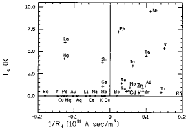
Figure 7: Superconducting critical temperature of the elements plotted versus the inverse Hall coefficient at low temperatures and high fields. Note that superconductivity is predominantly associated with a $positive$ Hall coefficient.

Another early empirical observation was made by Meissner and Schubert ms ; justi . They pointed out that the volume per valence electron (the difference between the atomic and ionic volume, divided by the number of conduction electrons per atom) is particularly small in superconducting elements compared to non-superconducting elements, with the smallest values associated with the highest transition temperatures. It is interesting that this criterion gives a qualitative understanding for why high critical temperatures are often achieved under high pressures, as discussed in several other papers in this Special Issue.

VIII summary and discussion

In this article we gave a brief review of superconductivity in elements, alloys and simple compounds at ambient pressure. These materials are generally believed to be described by the conventional BCS-Eliashberg theory, with the superconductivity caused by an effective electron-electron attraction resulting from the electron-phonon interaction, that overcomes the repulsive Coulomb interaction between electrons. The resulting superconducting state is s-wave, and the magnitude of the critical temperature is limited by the fact that phonon energy scales are much lower than electronic energy scales. The same theoretical framework is generally believed to explain why many elements, alloys and simple compounds do $not$ become superconducting at any temperature.

However, this raises the question: why are none of the non-conventional mechanisms proposed to apply to other classes of materials discussed in this Special Issue operative in the class of superconductors discussed in this article?

For example, it has been argued that spin fluctuations induced by strong Coulomb repulsion prevent conventional superconductivity from occurring in $Sc$ and $Pd$ pd . Why isn’t a spin-fluctuation mechanism scalreview proposed to be operative in several of the other classes of materials discussed in this Special Issue such as cuprates, pnictides, heavy fermions, Pu compounds, layered nitrides, organics, cobaltates and $Sr_{2}RuO_{4}$, operative in $Sc$ and $Pd$ and gives rise to superconductivity in them or in alloys or simple binary compounds with $Sc$ or $Pd$ as one of the components? Or, why doesn’t the $s\pm$ mechanism proposed to operate in iron pnictides operate in simple compounds that also have both hole-like and electron-like pieces to the Fermi surface?

We suggest that the question why none of the elements, alloys and simple compounds can take advantage of any of the non-conventional mechanisms operating in other materials is worth pondering, and that finding its answer could significantly advance our understanding of superconductivity in materials.

We also suggest that given the significant advances that have taken place in recent years in first principles calculations of electronic properties of materials gross ; new1 ; new2 , it should be possible using BCS-Eliashberg theory to better account for the $T_{c}$’s measured in elements, alloys and simple compounds, as well as the non-existence of superconductivity in many of these materials, than what was recounted in Sects. III and IV. For example, the theory is claimed to reproduce the $T_{c}=39K$ of $MgB_{2}$ from first principles to within $10\%$ without adjustable parameters liu ; choi ; floris ; margine , in rather complicated calculations where anharmonicity and anisotropy of the phonon spectrum is fully taken into account. It should be simpler and at least as successful to apply these techniques to elements and simple compounds. For a handful of elements and simple compounds this has recently been done and claimed to successfully reproduce the measured $T_{c}$’s gross ; margine ; gross2 ; gross3 . It should be systematically done for many elements and simple compounds. For example, can these methods reproduce the non-existence of superconductivity in the early and late transition metal series (e.g. $Sc$, $Y$, $Pd$, $Pt$) and the extremely low $T_{c}$ of $Li$ without additional ad-hoc assumptions such as a large $\mu^{*}$ as was done in the past pd ; papa ; cohen2 ; ashcr ? Can one computer program designed to calculate $T_{c}$ of binary compounds forming a cubic $NaCl$ structure such as the ones listed in Table IV, compute the critical temperature (including $T_{c}=0$) of binary compounds in such a structure by simply entering $Z_{1}$, $Z_{2}$ and $a$, the atomic number of each constituent and the lattice constant, with $no$ further adjustments? Approximate agreement with experiment for dozens of such elements and compounds would be an impressive validation of BCS-Eliashberg theory as the correct theory for the description of the superconductivity of conventional superconductors. On the other hand, significant disagreement would suggest that something is amiss with the present understanding of the validity of BCS-Eliashberg theory to describe superconductivity in simple materials validity .

References

- (1) H. Kamerlingh Onnes, Comm. Leiden 1911, Nr I22b, I24C; 1913, Nr 133a, I33C.
- (2) H. Kamerlingh Onnes, Comm. Leiden I913, Nr. I33a to I33 d.
- (3) W. Meissner, Ergebnisse der Exakten Naturwissenschaften 11, Springer, Berlin, p. 219 (1932).
- (4) H.G. Smith and J.O. Wilhelm, Rev. Mod. Phys. 7, 237 (1935).
- (5) E. Justi, Naturwissenschaften 33, 292 (1946).
- (6) J. Eisenstein, Rev. Mod. Phys. 26, 277 (1954).
- (7) C. Buzea and K. Robbie, Superconductor Science and Technology 18, R1 (2005).
- (8) Juha Tuoriniemi et al, Nature 447, 187 (2007).
- (9) See articles by J. Hamlin and K. Shimizu in this Special Issue.
- (10) W.J. de Haas and F. Juriaanse, Naturwiss. 19, 106 (1931).
- (11) W. Meissner, Z. Phys. 58, 570 (1929).
- (12) E. Justi, Phys. Zs. 42, 325 (1941).
- (13) J. de Launay and R. L. Dolecek, Phys. Rev. 72, 141 (1947).
- (14) H Fröhlich, Phys. Rev. 79, 845 (1950).
- (15) J. Bardeen, Rev. Mod. Phys. 23, 261 (1951).
- (16) H. Fröhlich, Rep. Prog. Phys. 24, 1 (1961).
- (17) For a different viewpoint see J. E. Hirsch, Physica Scripta 84, 045705 (2011).
- (18) E. Maxwell, Phys. Rev. 78 477 (1950).
- (19) C. A. Reynolds. B. Serin, W. H. Wright and L. B. Nesbitt, Phys. Rev. 78, 487 (1950).
- (20) M. Olsen, Nature 168, 246 (1951).
- (21) E. Maxwell, Phys. Rev. 86, 235 (1952).
- (22) M. A. Malik and B. A. Malik, American Journal of Condensed Matter Physics 2, 67 (2012).
- (23) J.W. Garland, Jr., Phys. Rev. Lett. 11 111 (1963); ibid, 114 (1963); Phys. Rev. 153, 460 (1963).
- (24) J. Bardeen, L.N. Cooper and J.R. Schrieffer, Phys. Rev. 106, 162 (1957); Phys. Rev. 108, 1175 (1957).
- (25) B. W. Roberts, J. Phys. Chem. Ref. Data 5, 581-821 (1976).
- (26) Theodore H Geballe, Robert H Hammond, Phillip M Wu, “What Tc Tells”, this Special Issue.
- (27) V.L. Ginzburg and L.D. Landau, Zh. Eksperim. i. Teor. Fiz. 20 1064 (1950). Importantly, Abrikosov [A.A. Abrikosov, Zh. Eksperim. i. Teor. Fiz 32, 1442 (1957) [Soviet Phys. - JETP 5, 1174 (1957)]] applied the Ginzburg-Landau theory to explain Type-II behavior, including early measurements of response of alloys to a magnetic field by L.V. Shubnikov, V.I. Khotkevich, Yu.D. Shepelev, Yu.N. Ryabinin, Zh. Eksperim. i. Teor. Fiz. 7, 221 (1937); translation in L.V. Shubnikov, V.I. Khotkevich, Yu.D. Shepelev, Yu.N. Ryabinin, Ukr. J. Phys. V. 53, 42 (2008) Special Issue.
- (28) A third critical field, , is also possible, predicted saint-james63 to occur at the surface of a type-II superconductor. This was verified experimentally for several type-II materials webb68 ; karasik70 and even for a type-I elemental superconductor mcevoy67 .
- (29) G.D. Cody and G.W. Webb, CRC Critical Reviews in Solid State and Materials Sciences, Vol 4, 27 (1973).
- (30) D. Saint-James and P. G. de Gennes, Phys. Lett. ??, 306 (1963).
- (31) G. W. Webb, Solid State Commun.6, 33 (1968).
- (32) V. R. Karasik and I. Yu. Shebalin, Soviet Phys. JETP 30, 1068 (1970).
- (33) J. P. McEvoy, D. P. Jones, and J. G. Park, Solid State Commun. 5, 641 (1967). It is possible in some Type I materials to supercool at the surface in fields below the surface nucleation field .
- (34) P.W. Anderson and B.T. Matthias, Science 144 373 (1964).
- (35) W.L. McMillan, Phys. Rev. 167 331 (1968).
- (36) L.N. Cooper, Phys. Rev. 104, 1189 (1956).
- (37) P. G. de Gennes, Superconductivity of Metals and Alloys (W.A. Benjamin, Inc. New York, 1966).
- (38) G.M. Eliashberg, Zh. Eksperim. i Teor. Fiz. 38 966 (1960); Soviet Phys. JETP 11 696 (1960).
- (39) H. Kamerlingh Onnes and W. Tuyn, Comm. Leiden 160b 451 (1923).
- (40) I. Giaever, Phys. Rev. Lett. 5 464 (1960).
- (41) L.C. Hebel and C.P. Slichter, Phys. Rev. 107, 901 (1957); Phys. Rev. 113, 1504 (1959); L.C. Hebel, Phys. Rev. 116, 79 (1959).
- (42) A.G. Redfield, Phys. Rev. Lett. 3, 85 (1959); A.G. Anderson and A.G. Redfield, Phys. Rev. 116 583 (1959).
- (43) B.L. Blackford and R.H. March, Can. J. Phys. 46, 141 (1968).
- (44) N.E. Phillips, Phys. Rev. 114 676 (1959).
- (45) See the many excellent reviews in Superconductivity, edited by R.D. Parks (Marcel Dekker, Inc., New York, 1969).
- (46) D.J. Scalapino, in Superconductivity, edited by R.D. Parks (Marcel Dekker, Inc., New York, 1969)p. 449.
- (47) W.L. McMillan and J.M. Rowell, in Superconductivity, edited by R.D. Parks (Marcel Dekker, Inc., New York, 1969)p. 561.
- (48) P.B. Allen and B. Mitrović, in Solid State Physics, edited by H. Ehrenreich, F. Seitz, and D. Turnbull (Academic, New York, 1982) Vol. 37, p.1.
- (49) D. Rainer, in Progress in Low Temperature Physics, Vol. 10, edited by D.F. Brewer (North-Holland, 1986), p.371.
- (50) J.P. Carbotte, Rev. Mod. Phys. 62 1027 (1990).
- (51) F. Marsiglio and J.P. Carbotte, ‘Electron-Phonon Superconductivity’, Review Chapter in Superconductivity, Conventional and Unconventional Superconductors, edited by K.H. Bennemann and J.B. Ketterson (Springer-Verlag, Berlin, 2008), pp. 73-162.
- (52) Note that retardation effects are taken into account in BCS theory in a very phenomenological way through the imposed cutoff. This cutoff is imposed in momentum space (not in frequency space), and because of the Fermi Liquid nature of BCS theory rainer86 this can be rewritten as a formulation in terms of Matsubara frequencies with a cutoff in this space, so it better resembles Eliashberg theory.
- (53) P.B. Allen and R.C. Dynes, Phys. Rev. B12 905 (1975); see also R.C. Dynes, Solid State Commun. 10 615 (1972).
- (54) N.N. Bogoliubov, N.V. Tolmachev, and D.V. Shirkov, A New Method in the Theory of Superconductivity, Consultants Bureau, Inc., New York (1959).
- (55) P. Morel and P.W. Anderson, Phys. Rev. 125 1263 (1962).
- (56) F. Marsiglio, J. Low. Temp. Phys. 87 659 (1992).
- (57) B. Mitrović, H.G. Zarate, and J.P. Carbotte, Phys. Rev. B29 184 (1984).
- (58) J.P. Carbotte and R.C. Dynes, Phys. Lett. A25, 685 (1967).
- (59) J.P. Carbotte and R.C. Dynes, “ Superconductivity in Simple Metals”, Phys. Rev. 172, 476 (1967).
- (60) J.M. Rowell, P.W. Anderson, and D.E. Thomas, Phys. Rev. Lett. 10 334 (1963).
- (61) J.R. Schrieffer, D.J. Scalapino and J.W. Wilkins, Phys. Rev. Lett. 10 336 (1963). D.J. Scalapino, J.R. Schrieffer and J.W. Wilkins, Phys. Rev. 148 263 (1966).
- (62) W.L. McMillan and J.M. Rowell, Phys. Rev. Lett. 14 108 (1965).
- (63) A.P. Roy and B.N. Brockhouse, Can. J. Phys. 48, 1781(1970).
- (64) D. Rainer and F.J. Culetto, Phys. Rev. B 19, 2540 (1979).
- (65) A. Knigavko and F. Marsiglio, Phys. Rev. B64, 172513 (2001).
- (66) P. B. Allen, Nature 335, 396 (1988).
- (67) R. D. Fowler. J. D. G. Lindsay, R. W. White. H. H. Hill and B. T. Matthias, Phys. Rev. Lett. 19, 892 (1967).
- (68) B. Stritzker and W. Buckel, Z. Physik 257, 1 (1972).
- (69) B.N. Ganguly, Z. Physik B22, 127 (1975).
- (70) B.M. Klein, E.N. Economu and D.A. Papaconstantopoulos, Phys. Rev. Lett. 39, 574 (1977).
- (71) See also V.V. Struzhkin, contribution to this volume.
- (72) A.P. Drozdov, M.I. Eremets and I.A. Troyan, “Conventional superconductivity at at high pressures”, arXiv:1412.0460 (2014).
- (73) “Handbook of Superconductivity”, edited by C.P. Poole, Jr, Academic Press, New York, 2000.
- (74) Also note that there are discrepancies in the reported experimental values of, for example, , in the literature.
- (75) P.B. Allen and M.L. Cohen, “Pseudopotential Calculation of the Mass Enhancement and Superconducting Transition Temperature of Simple Metals”, Phys. Rev. 187, 525 (1969).
- (76) T.L. Thorp et al, J. Low Temp. Phys. 3, 589 (1970).
- (77) A. Y. Liu and M. L. Cohen, Phys. Rev. B 44, 9678 (1991).
- (78) T. Bazhirov, J. Noffsinger, and M. L. Cohen, Phys. Rev. B84, 125122 (2011).
- (79) D. A. Papaconstantopoulos et al, “Calculation of the superconducting properties of 32 metals with ”, Phys. Rev. B 15, 4221 (1977).
- (80) G. D. Gaspari and B. L. Gyorffy, Phys. Rev. Lett. 28, 801 (1972)
- (81) A. D. Zdetsis, E. N. Economou and D. A. Papaconstantopoulos, Le Journal de Physique Lettres 46, L-253 (1979).
- (82) D. Glotzel, D. Rainer and H. R. Schober, Z. fur Physik B 35, 317 (1979).
- (83) J. S. Rajput, “Superconductivity in simple metals”, Phys. Stat. Sol. (b) 45, 287 (1971).
- (84) H. C. Gupta and B. B. Tripathi, “Pseudopotential calculation of superconducting transition temperature for simple metals”, Indian Journal of Pure and Applied Physics 10, 506 (1972).
- (85) S. C. Jain and C. M. Kachhava, “Electron-Phonon interaction and superconductivity in metals”, Phys. Stat. Sol. (b) 101, 619 (1980).
- (86) Y. G. Naidyuk et al, “Study of electron-phonon interaction in alkali metals”, Fizika Tverdogo Tela 22, 3665 (1980).
- (87) S. C. Jain and C. M. Kachhava, “Superconductivity in certain metals”, Indian Journal of Pure and Applied Physics 18, 489 (1980).
- (88) R. Sharma, K S. Sharma and L. Dass, “Linearized screened pseudopotential and superconducting state parameters of a number of metals”, Phys. Stat. Sol. (b) 133, 701(1986).
- (89) P. N. Gajjar, A. M. Vora and A. R. Jani, “Superconducting state parameters of metals”, Indian Journal of Physics and Proceedings of the Indian Association for the Cultivation of Science 78 775 (2004).
- (90) J. Yadev and S. M. Rafique, “Superconducting parameters of metals and alloys: HFP technique”, Indian Journal of Physics and Proceedings of the Indian Association for the Cultivation of Science 81, 161 (2007).
- (91) I. Skiyadneva et al, “Electron-phonon interaction in bulk Pb: Beyond the Fermi surface”, Phys. Rev. 85, 155115 (2012).
- (92) D. Rainer, “First principles calculations of in superconductors”, Physica B 109 110, 1671 (1982).
- (93) M. A. L. Marques, M. L ders, N. N. Lathiotakis, G. Profeta, A. Floris, L. Fast, A. Continenza, E. K. U. Gross, and S. Massidda, “Ab initio theory of superconductivity. II. Application to elemental metals”, Phys. Rev. 72, 024546 (2005).
- (94) B. T. Matthias, T. H. Geballe and V. B. Compton, Rev. Mod. Phys. 35, 1 (1963).
- (95) “Handbook of Superconductivity”, edited by C.P. Poole, Jr, Academic Press, New York, 2000. See in particular Chpt. 5 by C. P. Poole, Jr., P. C. Canfield and A. P. Ramirez and Chpt. 6 by R. Gladyshevskii and K. Cenzual.
- (96) S, V, Vonsovsky, Y. A. Izyumov and E¿ Z. Kurmaev, “Superconductivity of Transition Metals”, Springer, Berlin, 1982.
- (97) D.A: Papaconstantopoulos, W.E. Pickett, B.M. Klein and L. L. Boyer, Phys. Rev. B 31, 752 (1985).
- (98) W.E. Pickett, B.M. Klein and D.A: Papaconstantopoulos, “Theoretical prediction of MoN as a high t superconductor”, Physica B 107, 667 (1981).
- (99) G. Linker, R. Smithey and O. Meyer, “Superconductivity in MoN films with NaCI structure”, J. Phys. F 14, L115 (1984).
- (100) S. Blackburn, M. Cote, S. G. Louie and M. L. Cohen, Phys. Rev. B 84, 104506 (2011).
- (101) B. M. Klein and D. A. Papaconstantopoulos, Phys. Rev. Lett 32, 1193 (1974).
- (102) J.Noffsinger, F. Giustino, S. G. Louie and M. L. Cohen, Phys. Rev. B 77, 180507 (2008).
- (103) B.M. Klein, W. E. Pickett, D. A. Papaconstantopoulos, and L. L. Boyer, Phys. Rev. B 27, 6721 (1983).
- (104) Z. P. Yin, S. Y. Savrasov, and W. E. Pickett, Phys. Rev. B 74, 094519 (2006).
- (105) B.T. Matthias, “Empirical relation between superconductivity and the number of valence electrons per atom”, Phys. Rev. 97, 74 (1955).
- (106) D. Pines, Phys. Rev. 109, 280 (1958).
- (107) J. E. Hirsch and F. Marsiglio, Phys. Lett. A 140, 122 (1989); X. Q. Hong and J. E. Hirsch, Phys. Rev. B 46, 14702 (1992).
- (108) B. T. Matthias, Superconductivity in the Periodic System, Progress in Low Temperature Physics, Vol II, p. 138 (1957).
- (109) L. R. Testardi, Phys. Rev. 5 4342 (1972).
- (110) J. E. Hirsch, Phys. Lett. A 138, 83 (1989).
- (111) B. T. Matthias, “Criteria for Superconducting Transition Temperatures”, Physica 69, 54 (1973).
- (112) I. Kikoin and B. Lasarew, Nature 129, 58 (1932); Physikalische Zeitschrift der Sowjetunion 3, 351 (1933).
- (113) J. Linde, O. Rapp, Phys. Lett. A 70, 147 (1979)
- (114) I. M. Chapnik, Sov. Phys. Dokl. 6, 988 (1962).
- (115) I. M. Chapnik, Phys. Lett. A 72, 255 (1979).
- (116) I. M. Chapnik, J. Phys. F 13, 975 (1983).
- (117) I. M. Chapnik, Phys. Stat. Sol. (b) 123, K183 (1984).
- (118) I. K. Schuller, D. Hinks and R. J. Soulen Jr, Phys. Rev. B 25, 1981 (1982).
- (119) J. E. Hirsch, “Correlations between normal-state properties and superconductivity”, Phys. Rev. B 55, 9907 (1997).
- (120) W. Meissner and G. Schubert, “Zur Abrenzung der supraleitenden reinen Metalle gegenuber den anderen Elementen”, Sitz. der. Bayr. Akad. Wiss. Nat. Abstr. p 6 (1943).
- (121) G. Gladstone, M. A. Jensen and J. R. Schrieffer, ref. parks69 , p.665.
- (122) D. J. Scalapino, “A common thread: The pairing interaction for unconventional superconductors”, Rev. Mod. Phys. 84, 1383 (2012).
- (123) X. Gonze et al, “ABINIT: First-principles approach to material and nanosystem properties”, Computer Physics Communications 180, 2582 (2009).
- (124) J. Noffsinger et al, “A program for calculating the electron-phonon coupling using maximally localized Wannier functions”, Computer Physics Communications 181, 2140 (2010).
- (125) A. Y. Liu, I. I. Mazin, and J. Kortus, Phys. Rev. Lett. 87, 087005 (2001).
- (126) H. J. Choi, D. Roundy,, H. Sun, M. L. Cohen, and S. G. Louie, “First-principles calculation of the superconducting transition in within the anisotropic Eliashberg formalism”, Phys. Rev. B 66, 020513 (2002).
- (127) A. Floris et al, “Superconducting Properties of from First Principles”, Phys. Rev. Lett. 94, 037004 (2005).
- (128) E. R. Margine and F. Giustino, “Anisotropic Migdal-Eliashberg theory using Wannier functions”, Phys. Rev. B 87, 024505 (2013).
- (129) C Bersier et al, J. Phys. Cond. Matt. 21, 164209 (2009).
- (130) J. A. Flores-Livas and A. Sanna, arXiv:1411.4792 (2014).
- (131) C. F. Richardson and N. W. Ashcroft, Phys. Rev. B 55, 15130 (1997).
- (132) J. E. Hirsch, Phys. Scr. 80, 035702 (2009).