TTP15-05
Decoupling of heavy quarks at four loops and effective Higgs-fermion coupling

Abstract

We compute the decoupling constant $\zeta_{m}$ relating light quark masses of effective $n_{l}$-flavour QCD to $(n_{l}+1)$-flavour QCD to four-loop order. Immediate applications are the evaluation of the $\overline{\rm MS}$ charm quark mass with five active flavours and the bottom quark mass at the scale of the top quark or even at GUT scales. With the help of a low-energy theorem $\zeta_{m}$ can be used to obtain the effective coupling of a Higgs boson to light quarks with five-loop accuracy. We briefly discuss the influence on $\Gamma(H\to b\bar{b})$.

PACS numbers: 12.38.-t, 12.38.Bx, 14.65.Dw, 14.65.Fy

1 Introduction and notation

Perturbative calculations in QCD are quite advanced and have reached, at least for some observables, the four and even five-loop level (see Refs. [1, 2] for a recent review). This concerns in particular the renormalization group functions which have been computed at four loops in Refs. [3, 4, 5, 6, 7]. The first five-loop result has been obtained recently in Ref. [8] where the quark mass anomalous dimension has been computed to this order.

In order to consistently relate the quark masses and strong coupling constant evaluated at different energy scales, both the renormalization group functions and also the decoupling relations have to be available. The latter take care of integrating out heavy quark fields. In fact, $N$-loop running goes along with $(N-1)$-loop decoupling. Thus, besides the five-loop anomalous dimensions also the four-loop decoupling relations are needed. In Refs. [9, 10] a first step has been undertaken in this direction and the four-loop decoupling constant for $\alpha_{s}$ has been computed (although the five-loop beta function is not yet available). In this paper we complement the result by computing the four-loop corrections to the decoupling constant for the light quark masses, which supplements the five-loop result for $\gamma_{m}$ [8].

In Ref. [11] a formalism has been derived which allows for an effective calculation of the $N$-loop decoupling constants with the help of $N$-loop vacuum integrals. In the following we present the formulae which are relevant for the calculation of the quark mass decoupling constant.

The bare decoupling constant $\zeta_{m}^{0}$ is defined via the relation

$$m_{q}^{0\prime} = \zeta_{m}^{0}m_{q}^{0}\,,$$ (1)

where $m_{q}^{0}$ and $m_{q}^{0\prime}$ are the bare quark mass parameters in the full $n_{f}$- and effective $n_{l}(\equiv n_{f}-1)$-flavour theory. Introducing the renormalization constants in both theories leads to the equation

$$m_{q}^{\prime}(\mu) = \frac{Z_{m}}{Z_{m}^{\prime}}\zeta_{m}^{0}m_{q}(\mu)=\zeta_{m}m_{q}(\mu)\,,$$ (2)

which relates finite quantities and defines $\zeta_{m}$. Note that primed quantities depend on $\alpha_{s}^{(n_{l})}$ and non-primed quantities on $\alpha_{s}^{(n_{f})}$. Four-loop results for $Z_{m}$ and $Z_{m}^{\prime}$ can be found in Refs. [3, 4, 7] and $\zeta_{m}^{0}$ can be computed with the help of

$$\zeta_{m}^{0} = \frac{1-\Sigma_{S}^{0h}(0)}{1+\Sigma_{V}^{0h}(0)}\,,$$ (3)

where $\Sigma_{S}^{0h}(0)$ and $\Sigma_{V}^{0h}(0)$ are the scalar and vector parts of the light-quark self energy evaluated at zero external momentum. The superscript “h” reminds that one has to consider only the hard part which involves at least one propagator of the heavy quark.

In the next Section we discuss the calculation of $\zeta_{m}^{0}$ and its renormalization to arrive at $\zeta_{m}$. Section 3 applies a low-energy theorem to derive, from the four-loop result of $\zeta_{m}$, the effective Higgs-fermion coupling constant to five-loop order. We summarize our findings in Section 4.

2 Decoupling for light quark masses

Figure 1: Sample Feynman diagrams contributing to the hard part of the light-quark propagator up to four loops. Solid and curly lines denote quarks and gluons, respectively. At least one of the closed fermion loops needs to be the heavy quark.

In this section, we compute the decoupling constant $\zeta_{m}^{0}$ and combine it with the four-loop result for $Z_{m}$ to obtain the finite quantity $\zeta_{m}$. The computation of $\zeta_{m}^{0}$ requires the knowledge of the hard contribution to the scalar and vector part of the light-quark propagator, see Fig. 1 for sample Feynman diagrams. The first non-vanishing contribution arises at two loops where one diagram contributes. At three-loop order there are 25 and at four loops we have 765 Feynman diagrams.

The perturbative expansion of Eq. (3) to four loops leads to

$$\zeta_{m}^{0} = 1-\Sigma_{S}^{0h}(0)-\Sigma_{V}^{0h}(0)+\Sigma_{V}^{0h}(0)\left[\Sigma_{S}^{0h}(0)+\Sigma_{V}^{0h}(0)\right]+\ldots\,,$$ (4)

where in the last term on the right-hand side only two-loop expressions for $\Sigma_{S}^{0h}(0)$ and $\Sigma_{V}^{0h}(0)$ have to be inserted.

We generate the Feynman diagrams with the help of QGRAF [12]. FORM [13, 14] code is then generated by passing the output via q2e [15, 16], which transforms Feynman diagrams into Feynman amplitudes, to exp [15, 16]. After processing the latter one obtains the result as a linear combination of scalar functions which have a one-to-one relation to the underlying topology of the diagram. The functions contain the exponents of the involved propagators as arguments. At this point one has a large number of different functions. Thus, in the next step one passes them to a program which implements the Laporta algorithm [17] and performs a reduction to a small number of so-called master integrals. We use, for the latter step, the C++ program FIRE [18]. Our four-loop result is expressed in terms of 13 master integrals which we take from Ref. [19] (see also [20, 21, 22] and references therein). All $\epsilon$ coefficients are known analytically in the literature except the $\epsilon^{3}$ term of integral $J_{6,2}$ (in the notation from Ref. [19]) which has been provided from [23].

Note that for our calculation we have used a general gauge parameter $\xi$ of the gluon propagator. At four loops, in intermediate steps terms up to order $\xi^{6}$ are present, however, in the final result for $\zeta_{m}^{0}$ all $\xi$ terms drop out. The last term on the right-hand side of Eq. (4) is separately $\xi$-independent since at two loops $\Sigma_{S}^{0h}(0)$ and $\Sigma_{V}^{0h}(0)$ are individually $\xi$-independent. The results up to three-loop order have been checked with the help of MATAD [24] which avoids the use of the program FIRE since it implements the explicit solution of the recurrence relations.

To obtain $\zeta_{m}^{0}$ we have to renormalize $\alpha_{s}$ and the heavy quark mass $m_{h}$ to two-loop order. The corresponding $\overline{\rm MS}$ counterterms are well-known (see, e.g.. Ref. [7]). $\zeta_{m}^{0}$ still contains poles in $\epsilon$ which are removed by multiplying with the factor $Z_{m}/Z_{m}^{\prime}$ (see, Eq. (2)) which is needed to four-loop order [3, 4, 7]. Note that $Z_{m}^{\prime}$ depends on the strong coupling constant of the effective theory, $\alpha_{s}^{(n_{l})}$, whereas $Z_{m}$ and $\zeta_{m}^{0}$ are expressed in terms of $\alpha_{s}^{(n_{l}+1)}$. In order to achieve the cancellation of the $\epsilon$ poles the same coupling constant has to be used in all three quantities. We have decided to replace $\alpha_{s}^{(n_{l})}$ in favour of $\alpha_{s}^{(n_{l}+1)}$ which is done using the corresponding decoupling constant $\zeta_{\alpha_{s}}$ up three-loop order [11]. Note, however, that higher order terms in $\epsilon$ are also needed since $\zeta_{\alpha_{s}}$ gets multiplied by poles present in $Z_{m}^{\prime}$. Up to two-loop order they can be found in Refs. [25, 26]; the three-loop terms of order $\epsilon$ can be extracted from Refs. [9, 10].

Our final result for the decoupling constant parametrized in terms of the $\overline{\rm MS}$ heavy quark mass, $m_{h}\equiv m_{h}(\mu)$, reads

$$\zeta_{m}^{\overline{\rm MS}}=$$ (5)

$$\!\!\!\!\!\!\!\!\!\!\!\!1+\left(\frac{\alpha_{s}^{(n_{f})}}{\pi}\right)^{2}\left(\frac{89}{432}-\frac{5}{36}\ln\frac{\mu^{2}}{m_{h}^{2}}+\frac{1}{12}\ln^{2}\frac{\mu^{2}}{m_{h}^{2}}\right)+\left(\frac{\alpha_{s}^{(n_{f})}}{\pi}\right)^{3}\left[\frac{2951}{2916}+\frac{1}{9}\zeta(2)\ln^{2}2\right.$$

$${}-\frac{1}{54}\ln^{4}2-\frac{407}{864}\zeta(3)+\frac{103}{72}\zeta(4)-\frac{4}{9}a_{4}-\left(\frac{311}{2592}+\frac{5}{6}\zeta(3)\right)\ln\frac{\mu^{2}}{m_{h}^{2}}+\frac{175}{432}\ln^{2}\frac{\mu^{2}}{m_{h}^{2}}$$

$${}\left.+\frac{29}{216}\ln^{3}\frac{\mu^{2}}{m_{h}^{2}}+n_{l}\left(\frac{1327}{11664}-\frac{2}{27}\zeta(3)-\frac{53}{432}\ln\frac{\mu^{2}}{m_{h}^{2}}-\frac{1}{108}\ln^{3}\frac{\mu^{2}}{m_{h}^{2}}\right)\right]$$

$${}+\left(\frac{\alpha_{s}^{(n_{f})}}{\pi}\right)^{4}\Bigg{[}\frac{131968227029}{3292047360}-\frac{1924649}{4354560}\ln^{4}2+\frac{59}{1620}\ln^{5}2+\frac{1924649}{725760}\zeta(2)\ln^{2}2$$

$${}-\frac{59}{162}\zeta(2)\ln^{3}2-\frac{353193131}{40642560}\zeta(3)+\frac{1061}{576}\zeta(3)^{2}+\frac{16187201}{580608}\zeta(4)-\frac{725}{108}\zeta(4)\ln 2$$

$${}-\frac{59015}{1728}\zeta(5)-\frac{3935}{432}\zeta(6)-\frac{1924649}{181440}a_{4}-\frac{118}{27}a_{5}+\left(-\frac{2810855}{373248}-\frac{31}{216}\ln^{4}2\right.$$

$${}\left.+\frac{31}{36}\zeta(2)\ln^{2}2-\frac{373261}{27648}\zeta(3)+\frac{4123}{288}\zeta(4)+\frac{575}{72}\zeta(5)-\frac{31}{9}a_{4}\right)\ln\frac{\mu^{2}}{m_{h}^{2}}$$

$${}+\left(\frac{51163}{10368}-\frac{155}{48}\zeta(3)\right)\ln^{2}\frac{\mu^{2}}{m_{h}^{2}}+\frac{301}{324}\ln^{3}\frac{\mu^{2}}{m_{h}^{2}}+\frac{305}{1152}\ln^{4}\frac{\mu^{2}}{m_{h}^{2}}$$

$${}+n_{l}\left(-\frac{2261435}{746496}+\frac{49}{2592}\ln^{4}2-\frac{1}{270}\ln^{5}2-\frac{49}{432}\zeta(2)\ln^{2}2+\frac{1}{27}\zeta(2)\ln^{3}2\right.$$

$${}\left.-\frac{1075}{1728}\zeta(3)-\frac{1225}{3456}\zeta(4)+\frac{49}{72}\zeta(4)\ln 2+\frac{497}{288}\zeta(5)+\frac{49}{108}a_{4}+\frac{4}{9}a_{5}\right.$$

$${}\left.+\left(\frac{16669}{31104}+\frac{1}{108}\ln^{4}2-\frac{1}{18}\zeta(2)\ln^{2}2+\frac{221}{576}\zeta(3)-\frac{163}{144}\zeta(4)+\frac{2}{9}a_{4}\right)\ln\frac{\mu^{2}}{m_{h}^{2}}\right.$$

$${}\left.-\frac{7825}{10368}\ln^{2}\frac{\mu^{2}}{m_{h}^{2}}-\frac{23}{288}\ln^{3}\frac{\mu^{2}}{m_{h}^{2}}-\frac{5}{144}\ln^{4}\frac{\mu^{2}}{m_{h}^{2}}\right)+n_{l}^{2}\left(\frac{17671}{124416}-\frac{5}{864}\zeta(3)\right.$$

$${}\left.-\frac{7}{96}\zeta(4)+\left(-\frac{3401}{46656}+\frac{7}{108}\zeta(3)\right)\ln\frac{\mu^{2}}{m_{h}^{2}}+\frac{31}{1296}\ln^{2}\frac{\mu^{2}}{m_{h}^{2}}+\frac{1}{864}\ln^{4}\frac{\mu^{2}}{m_{h}^{2}}\right)\Bigg{]}$$

$$\stackrel{{\scriptstyle\mu=m_{h}}}{{=}} \mbox{}1+\left(\frac{\alpha_{s}^{(n_{f})}(m_{h})}{\pi}\right)^{2}0.2060+\left(\frac{\alpha_{s}^{(n_{f})}(m_{h})}{\pi}\right)^{3}\left(1.848+0.02473n_{l}\right)$$

$$\mbox{}+\left(\frac{\alpha_{s}^{(n_{f})}(m_{h})}{\pi}\right)^{4}\left(6.850-1.466n_{l}+0.05616n_{l}^{2}\right)\,,$$

with $\alpha_{s}^{(n_{f})}\equiv\alpha_{s}^{(n_{f})}(\mu)$. In the analytic expression $\zeta(n)$ denotes the Riemann zeta function evaluated at $n$ and $a_{n}=\mbox{Li}_{n}(1/2)$.

Often it is convenient to express $\zeta_{m}$ in terms of the on-shell heavy quark mass, $M_{h}$. The corresponding analytic expressions are obtained from Eq. (5) with the help of the two-loop relation between $m_{h}(\mu)$ and $M_{h}$ which can be found in Refs. [27, 28, 29]. We refrain from showing the corresponding analytic result and restrict the presentation to the numerical expression which is given by

$$\zeta_{m}^{\rm OS} = 1+\left(\frac{\alpha_{s}^{(n_{f})}}{\pi}\right)^{2}\left(0.2060-0.1389\ln\frac{\mu^{2}}{M_{h}^{2}}+0.08333\ln^{2}\frac{\mu^{2}}{M_{h}^{2}}\right)$$ (6)

$$\mbox{}+\left(\frac{\alpha_{s}^{(n_{f})}}{\pi}\right)^{3}\left[1.477-0.9550\ln\frac{\mu^{2}}{M_{h}^{2}}+0.7384\ln^{2}\frac{\mu^{2}}{M_{h}^{2}}+0.1343\ln^{3}\frac{\mu^{2}}{M_{h}^{2}}\right.$$

$$\left.\mbox{}+n_{l}\left(0.02473-0.1227\ln\frac{\mu^{2}}{M_{h}^{2}}-0.009259\ln^{3}\frac{\mu^{2}}{M_{h}^{2}}\right)\right]+\left(\frac{\alpha_{s}^{(n_{f})}}{\pi}\right)^{4}\bigg{[}\left.0.2233\right.$$

$$\left.\mbox{}+2.674\ln\frac{\mu^{2}}{M_{h}^{2}}+6.227\ln^{2}\frac{\mu^{2}}{M_{h}^{2}}+2.165\ln^{3}\frac{\mu^{2}}{M_{h}^{2}}+0.2648\ln^{4}\frac{\mu^{2}}{M_{h}^{2}}\right.$$

$$\left.\mbox{}+n_{l}\left(-1.504-0.6470\ln\frac{\mu^{2}}{M_{h}^{2}}-0.9260\ln^{2}\frac{\mu^{2}}{M_{h}^{2}}-0.1632\ln^{3}\frac{\mu^{2}}{M_{h}^{2}}\right.\right.$$

$$\left.\left.\mbox{}-0.03472\ln^{4}\frac{\mu^{2}}{M_{h}^{2}}\right)+n_{l}^{2}\left(0.05616+0.005016\ln\frac{\mu^{2}}{M_{h}^{2}}+0.02392\ln^{2}\frac{\mu^{2}}{M_{h}^{2}}\right.\right.$$

$$\left.\left.\mbox{}+0.001157\ln^{4}\frac{\mu^{2}}{M_{h}^{2}}\right)\bigg{]}\right.\,.$$

On the webpage [30] we provide analytic results in computer-readable form for a general $SU(N_{c})$ gauge group.

In the remaining part of this section we discuss two applications which involve the evaluation of light quark masses at high scales. In the first one we compute the running bottom quark mass at the scale $\mu=M_{t}$, where $M_{t}$ is the top quark pole mass. $m_{b}(M_{t})$ appears as an intermediate step in analyses concerned with Yukawa coupling unification. Here the role of the heavy quark is taken over by the top quark. In the second application we cross the bottom threshold and evaluate the charm quark mass for $\mu=M_{Z}$ using $m_{c}^{(4)}(3~{}\mbox{GeV})$ as input. As input parameters for the numerical analyses we use [31, 32]

$$\alpha_{s}^{(5)}(M_{Z}) = 0.1185\,,$$

$$m_{b}^{(5)}(m_{b}^{(5)}) = 4.163~{}\mbox{GeV}\,,$$

$$m_{c}^{(4)}(3~{}\mbox{GeV}) = 0.986~{}\mbox{GeV}\,.$$ (7)

As a first phenomenological application we consider the evaluation of the bottom quark mass at the scale of the top quark with six active flavours using $m_{b}^{(5)}(m_{b}^{(5)})$ as input. We are interested in the dependence of $m_{b}^{(6)}(M_{t})$ on the decoupling scale of the top quark. Since this scale is unphysical it should get weaker after including higher order corrections. Our results, which are shown in Fig. 2(a), are obtained using the following scheme, where $N\in\{1,2,3,4,5\}$ refers to the number of loops:

• Use $N$-loop running: $m_{b}^{(5)}(m_{b}^{(5)})\to m_{b}^{(5)}(\mu_{t}^{\rm dec})$

• Use $(N-1)$-loop decoupling: $m_{b}^{(5)}(\mu_{t}^{\rm dec})\to m_{b}^{(6)}(\mu_{t}^{\rm dec})$

• Use $N$-loop running $m_{b}^{(6)}(\mu_{t}^{\rm dec})\to m_{b}^{(6)}(M_{t})$

The values for $\alpha_{s}$ involved in this procedure, $\alpha_{s}^{(5)}(m_{b}^{(5)}(m_{b}^{(5)}))$, $\alpha_{s}^{(5)}(\mu_{t}^{\rm dec})$, $\alpha_{s}^{(6)}(\mu_{t}^{\rm dec})$, and $\alpha_{s}^{(6)}(M_{t})$, are obtained from $\alpha_{s}^{(5)}(M_{Z})$ using the same loop-order for the running and decoupling as described above for the bottom quark mass.

In Fig. 2(a) $m_{b}^{(6)}(M_{t})$ is shown as a function of the scale $\mu_{t}^{\rm dec}$ where the transition from five- to six-flavour QCD is performed normalized to the on-shell top quark mass. For the on-shell top quark mass we choose $M_{t}=173.34$ GeV [33]. We vary $\mu_{t}^{\rm dec}/M_{t}$ by a factor of 10 around the central scale $\mu_{t}^{\rm dec}/M_{t}=1$. The one-loop result leads to $m_{b}^{(6)}(M_{t})\approx 2.9$ GeV and is not shown in the plot. One observes that already the result where two-loop running is used (short-dashed line) shows only a weak dependence on $\mu_{t}^{\rm dec}$. It becomes even weaker at three and four loops (results with higher perturbative order have longer dashes) and results in an almost flat curve at five loops (solid line) which can barely be distinguished from the four-loop curve. The five-loop results depends on the unknown five-loop coefficient $\beta_{4}$ of the beta function. Our default choice in Fig. 2(a) is $\beta_{4}=100\beta_{0}$ ($\beta_{0}=11/4-n_{f}/6$) which is numerically close to the Padé estimate obtained in Ref. [34]. For $\beta_{4}=0$ and $\beta_{4}=200\beta_{0}$ one observes a shift of the five-loop result by about $+0.5$ MeV and $-0.5$ MeV, respectively.

It is interesting to look at the shift on $m_{b}^{(6)}(M_{t})$ at the central scale $\mu_{\rm dec}=M_{t}$. The two-, three- and four-loop curves lead to shifts of about $-201$ MeV, $-21$ MeV and $-2$ MeV, respectively. For $\beta_{4}=100\beta_{0}$ the five-loop result leads to a shift of about $-0.5$ MeV.

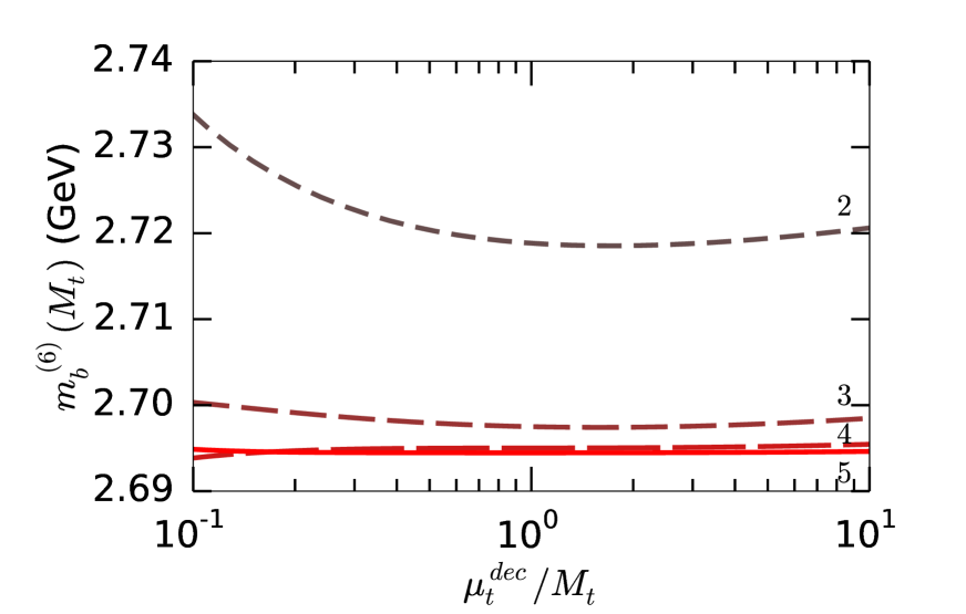
(a)

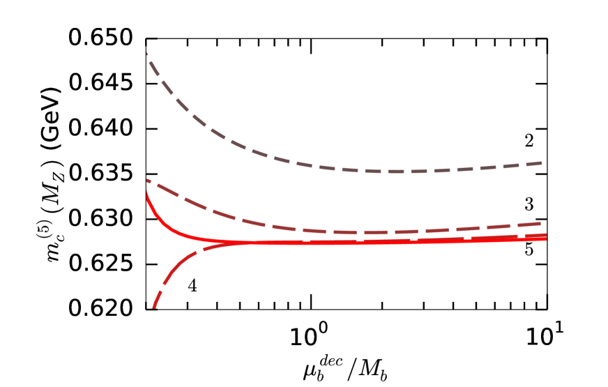
(b)

Figure 2: $m_{b}^{(6)}(M_{t})$ as a function of $\mu_{t}^{\rm dec}$ (a) and $m_{c}^{(5)}(M_{Z})$ as a function of $\mu_{b}^{\rm dec}$ (b). The numbers indicate the loop order used for the running.

In a second application we consider the evaluation of $m_{c}^{(5)}(M_{Z})$ with $m_{c}^{(4)}(3~{}\mbox{GeV})$ as input. The calculation proceeds in analogy to the bottom quark case discussed before, where for the on-shell bottom quark mass we use the value $M_{b}=4.7$ GeV. Our results are shown in Fig. 2(b). Again one observes a flattening of the curves after including higher order corrections. However, for $\mu_{b}^{\rm dec}\approx 1$ GeV, which corresponds to the left border of Fig. 2(b), all curves show a strong variation which indicates the breakdown of perturbation theory for small scales. Around $\mu_{b}^{\rm dec}/M_{b}\;\hbox to0.0pt{\lower 3.5pt\hbox{$\mathchar 0\relax\sim$}\hss}\raise 1.0pt\hbox{$>$}\;0.3$ both the four- and five-loop curves are basically flat.

At the central scale $\mu_{b}^{\rm dec}=M_{b}$ one observes shifts in $m_{c}^{(5)}(M_{Z})$ of $-55$ MeV, $-7$ MeV and $-1$ MeV after including two-, three- and four-loop running accompanied by one-, two- and three-loop decoupling. The shift at five loops is below 1 MeV for $\beta_{4}=100\beta_{0}$ but also for $\beta_{4}=0$ and $\beta_{4}=200\beta_{0}$.

3 Low-energy theorem: Higgs-fermion coupling

The effective Lagrangian describing the coupling of a Higgs boson to gluons and light quarks can be written in the form

$${\cal L}_{\rm eff} = -\frac{H^{0}}{v^{0}}\left(C_{1}{\cal O}_{1}^{\prime}+C_{2}{\cal O}_{2}^{\prime}\right)\,,$$ (8)

where the effective operators, which are constructed from light degrees of freedom [35], are given by

$${\cal O}^{\prime}_{1} = \left(G^{a,\mu\nu}\right)^{2}\,,$$

$${\cal O}^{\prime}_{2} = \sum_{i=1}^{n_{l}}m_{q_{i}}^{0\prime}\bar{\psi}_{q_{i}}^{0\prime}\psi_{q_{i}}^{0\prime}\,.$$ (9)

The residual dependence on the mass $m_{h}$ of the heavy quark $h$ is contained in the coefficient functions $C_{1}^{0}$ and $C_{2}^{0}$. In Eq. (8) $H$ denotes the Higgs field and $v$ the vacuum expectation value. The superscript “0” reminds us that the corresponding quantities are bare. For the renormalization of $C_{1}^{0},C_{2}^{0},{\cal O}_{1}^{\prime}$ and ${\cal O}_{2}^{\prime}$ we refer to Ref. [35, 11]; for the purpose of this paper it is of no further relevance. In Ref. [11] a low-energy theorem has been derived which relates the computation of the renormalized coefficient function $C_{2}$ to derivatives of $\zeta_{m}$ w.r.t. the heavy mass $m_{h}$. It is given by

$$C_{2} = 1+\frac{\partial\ln\zeta_{m}}{\partial\ln m_{h}}\,.$$ (10)

It should be stressed that Eq. (10) is valid to all orders in $\alpha_{s}$. Note that Eq. (10) contains the derivative w.r.t. $\ln m_{h}$ and furthermore the $m_{h}$ dependence of $C_{2}$ appears in the form $\ln(\mu/m_{h})$. Thus we can exploit renormalization group techniques to construct all logarithmic terms of the next, not computed perturbative order. In particular, on the basis of our four-loop calculation for $\zeta_{m}$ we can compute $C_{2}$ to five-loop accuracy using the recently computed five-loop result for the quark mass anomalous dimension [8]. Note that the four-loop anomalous dimensions have been computed in Refs. [3, 4] ($\gamma_{m}$) and Refs. [5, 6] ($\beta$), respectively.

Inserting $\zeta_{m}^{\overline{\rm MS}}$ into Eq. (10) we obtain the following result

$$C_{2}^{\overline{\rm MS}} = 1+\left(\frac{\alpha_{s}^{(n_{f})}}{\pi}\right)^{2}0.2778+\left(\frac{\alpha_{s}^{(n_{f})}}{\pi}\right)^{3}\left(2.243+0.2454\,n_{l}\right)$$ (11)

$$\mbox{}+\left(\frac{\alpha_{s}^{(n_{f})}}{\pi}\right)^{4}\left(2.180+0.3096\,n_{l}-0.01003\,n_{l}^{2}\right)$$

$$\mbox{}+\left(\frac{\alpha_{s}^{(n_{f})}}{\pi}\right)^{5}\left(66.71+13.44\,n_{l}-3.642\,n_{l}^{2}+0.07556\,n_{l}^{3}\right)\,,$$

where we have chosen $\mu=m_{h}$ to obtain more compact expressions. Analytic result valid for general $\mu$ are provided from [30].

In practice, one often encounters the situation where $C_{2}$ has to be inserted in a formula expressed in terms of $\alpha_{s}^{(n_{l})}$. If we furthermore transform the heavy quark mass to the on-shell scheme we obtain for $\mu=M_{h}$

$$C_{2}^{\rm OS} = 1+\left(\frac{\alpha_{s}^{(n_{l})}}{\pi}\right)^{2}0.2778+\left(\frac{\alpha_{s}^{(n_{l})}}{\pi}\right)^{3}\left(1.355+0.2454\,n_{l}\right)$$ (12)

$$\mbox{}+\left(\frac{\alpha_{s}^{(n_{l})}}{\pi}\right)^{4}\left(-12.13+1.004\,n_{l}-0.01003\,n_{l}^{2}\right)$$

$$\mbox{}+\left(\frac{\alpha_{s}^{(n_{l})}}{\pi}\right)^{5}\left(-140.9+44.20\,n_{l}-4.332\,n_{l}^{2}+0.07556\,n_{l}^{3}\right)\,.$$

Let us briefly discuss the influence of $C_{2}$ on the Higgs boson decay to bottom quarks where the role of the heavy quark is taken over by the top quark. We consider the contributions proportional to $(C_{2})^{2}$ from Eq. (8) and use the result for the massless correlator from Ref. [36]. For convenience we identify the renormalization scale with the Higgs boson mass and set $\mu=M_{H}$. Then the decay rate of the Standard Model Higgs boson to bottom quarks can be written in the form

$$\Gamma(H\to b\bar{b}) = \frac{G_{F}M_{H}^{2}}{4\sqrt{2}\pi}m_{b}^{2}(M_{H})\,R(M_{H})\,,$$ (13)

$$R(M_{H}) = 1+5.667\left(\frac{\alpha_{s}}{\pi}\right)+\left(29.147+0.991\right)\left(\frac{\alpha_{s}}{\pi}\right)^{2}+\left(41.758+13.105\right)\left(\frac{\alpha_{s}}{\pi}\right)^{3}$$

$$\mbox{}+\left(-825.7+50.7\right)\left(\frac{\alpha_{s}}{\pi}\right)^{4}+\left(r_{5}+224.8\right)\left(\frac{\alpha_{s}}{\pi}\right)^{5}$$

$$= 1+0.20400+\left(0.03777+0.00128\right)+\left(0.00195+0.00061\right)$$

$$\mbox{}+\left(-0.00139+0.00009\right)+\left(0.00000006r_{5}+0.00001\right)\,,$$

with $\alpha_{s}\equiv\alpha_{s}(M_{H})\approx 0.1131$. The first number in the round brackets in Eq. (3) corresponds to the case $C_{2}=1$ [36] and the second one to the contribution from $(C_{2}-1)$. At three-loop order the top quark induced part amounts to about 30%, at order $\alpha_{s}^{4}$ only 6%. Note that the massless correlator at order $\alpha_{s}^{5}$, denoted by $r_{5}$ in Eq. (3), is currently unknown. The $\alpha_{s}^{5}$ term in Eq. (3) origins from the five-loop contribution in Eq. (12) and products of lower-order contributions.

Note that in this consideration the contribution of $C_{1}$ (cf. Eq. (8)) has been neglected. The corresponding corrections of order $\alpha_{s}^{3}$ can be found in Ref. [37]. Corrections of order $\alpha_{s}^{4}$ which are proportional to $C_{1}C_{2}$ require the evaluation of massless four-loop two-point functions and are currently unknown. Corrections of order $\alpha_{s}^{5}$ to the Higgs boson decay rate involving $(C_{1})^{2}$ have been computed in Ref. [38].

In Refs. [9, 10] the five-loop result for $C_{1}$ is given in terms of $\alpha_{s}^{(n_{f})}$ and the $\overline{\rm MS}$ quark mass. We complement this result by $C_{1}$ parametrized in terms of the effective coupling constant and the on-shell mass:

$$C_{1}^{\rm OS} = -\frac{1}{12}\frac{\alpha_{s}^{(n_{l})}}{\pi}\left\{1+\left(\frac{\alpha_{s}^{(n_{l})}}{\pi}\right)2.750+\left(\frac{\alpha_{s}^{(n_{l})}}{\pi}\right)^{2}\left(9.642-0.6979n_{l}\right)\right.$$ (15)

$$\left.\mbox{}+\left(\frac{\alpha_{s}^{(n_{l})}}{\pi}\right)^{3}\left(50.54-6.801n_{l}-0.2207n_{l}^{2}\right)+\left(\frac{\alpha_{s}^{(n_{l})}}{\pi}\right)^{4}\bigg{[}-625.2+149.8n_{l}\right.$$

$$\left.\mbox{}-3.090n_{l}^{2}-0.07752n_{l}^{3}+6\left(\beta_{4}^{(n_{l})}-\beta_{4}^{(n_{l}+1)}\right)\bigg{]}\right\}\,,$$

where $\mu=M_{t}$ has been chosen. The analytic version in computer-readable form can again be found in [30].

4 Summary and conclusions

In this paper we compute the four-loop corrections to the decoupling constant for light quark masses, $\zeta_{m}$, which has to be applied every time heavy quark thresholds are crossed. It constitutes a fundamental constant of QCD and accompanies the five-loop quark anomalous dimension [8] in the “running and decoupling” procedure. Our results complete the calculation of the four-loop decoupling constants which has been started in Refs. [9, 10]. Note that the five-loop corrections to the QCD beta function, which is needed to establish relations between $\alpha_{s}(\mu)$ and $m_{q}(\mu)$ at low and high energy scales, is still missing.

As a by-product of our calculation we obtain the effective coupling of a scalar Higgs boson and light quarks to five-loop order. It is obtained from $\zeta_{m}$ with the help of an all-order low-energy theorem. We briefly investigate the influence on $\Gamma(H\to b\bar{b})$.

References

• [1] P. A. Baikov, K. G. Chetyrkin and J. H. Kühn, arXiv:1501.06739 [hep-ph].
• [2] K. G. Chetyrkin, J. H. Kühn, M. Steinhauser and C. Sturm, arXiv:1502.00509 [hep-ph].
• [3] K. G. Chetyrkin, Phys. Lett. B 404 (1997) 161 [hep-ph/9703278].
• [4] J. A. M. Vermaseren, S. A. Larin and T. van Ritbergen, Phys. Lett. B 405 (1997) 327 [hep-ph/9703284].
• [5] T. van Ritbergen, J. A. M. Vermaseren and S. A. Larin, Phys. Lett. B 400 (1997) 379 [hep-ph/9701390].
• [6] M. Czakon, Nucl. Phys.  B 710 (2005) 485 [hep-ph/0411261].
• [7] K. G. Chetyrkin, Nucl. Phys. B 710 (2005) 499 [hep-ph/0405193].
• [8] P. A. Baikov, K. G. Chetyrkin and J. H. Kühn, JHEP 1410 (2014) 76 [arXiv:1402.6611 [hep-ph]].
• [9] Y. Schroder and M. Steinhauser, JHEP 0601 (2006) 051 [hep-ph/0512058].
• [10] K. G. Chetyrkin, J. H. Kühn and C. Sturm, Nucl. Phys. B 744 (2006) 121 [hep-ph/0512060].
• [11] K. G. Chetyrkin, B. A. Kniehl and M. Steinhauser, Nucl. Phys. B 510 (1998) 61 [hep-ph/9708255].
• [12] P. Nogueira, J. Comput. Phys.  105 (1993) 279.
• [13] J. A. M. Vermaseren, arXiv:math-ph/0010025.
• [14] J. Kuipers, T. Ueda, J. A. M. Vermaseren and J. Vollinga, Comput. Phys. Commun.  184 (2013) 1453 [arXiv:1203.6543 [cs.SC]].
• [15] R. Harlander, T. Seidensticker and M. Steinhauser, Phys. Lett. B 426 (1998) 125 [hep-ph/9712228].
• [16] T. Seidensticker, hep-ph/9905298.
• [17] S. Laporta, Int. J. Mod. Phys. A 15 (2000) 5087 [hep-ph/0102033].
• [18] A. V. Smirnov, arXiv:1408.2372 [hep-ph].
• [19] R. N. Lee and I. S. Terekhov, JHEP 1101 (2011) 068 [arXiv:1010.6117 [hep-ph]].
• [20] S. Laporta, Phys. Lett. B 549 (2002) 115 [hep-ph/0210336].
• [21] Y. Schroder and A. Vuorinen, JHEP 0506 (2005) 051 [hep-ph/0503209].
• [22] K. G. Chetyrkin, M. Faisst, C. Sturm and M. Tentyukov, Nucl. Phys. B 742 (2006) 208 [hep-ph/0601165].
• [23] R. Lee, private communication.
• [24] M. Steinhauser, Comput. Phys. Commun.  134 (2001) 335 [hep-ph/0009029].
• [25] A. G. Grozin, P. Marquard, J. H. Piclum and M. Steinhauser, Nucl. Phys. B 789 (2008) 277 [arXiv:0707.1388 [hep-ph]].
• [26] A. G. Grozin, M. Hoeschele, J. Hoff, M. Steinhauser, JHEP 1109 (2011) 066 [arXiv:1107.5970 [hep-ph]].
• [27] N. Gray, D. J. Broadhurst, W. Grafe and K. Schilcher, Z. Phys. C 48 (1990) 673.
• [28] K. G. Chetyrkin and M. Steinhauser, Nucl. Phys. B 573 (2000) 617 [hep-ph/9911434].
• [29] K. Melnikov and T. v. Ritbergen, Phys. Lett. B 482 (2000) 99 [hep-ph/9912391].
• [30] http://www.ttp.kit.edu/Progdata/ttp15/ttp15-005
• [31] K. A. Olive et al. [Particle Data Group Collaboration], Chin. Phys. C 38 (2014) 090001.
• [32] K. G. Chetyrkin, J. H. Kühn, A. Maier, P. Maierhofer, P. Marquard, M. Steinhauser and C. Sturm, Phys. Rev. D 80 (2009) 074010 [arXiv:0907.2110 [hep-ph]].
• [33] [ATLAS and CDF and CMS and D0 Collaborations], arXiv:1403.4427 [hep-ex].
• [34] J. R. Ellis, I. Jack, D. R. T. Jones, M. Karliner and M. A. Samuel, Phys. Rev. D 57 (1998) 2665 [hep-ph/9710302].
• [35] V. P. Spiridonov, preprint IYaI-P-0378, 1984.
• [36] P. A. Baikov, K. G. Chetyrkin and J. H. Kühn, Phys. Rev. Lett.  96 (2006) 012003 [hep-ph/0511063].
• [37] K. G. Chetyrkin and M. Steinhauser, Phys. Lett. B 408 (1997) 320 [hep-ph/9706462].
• [38] P. A. Baikov and K. G. Chetyrkin, Phys. Rev. Lett.  97 (2006) 061803 [hep-ph/0604194].