Anisotropy of third-order structure functions in MHD turbulence

Abstract

The measure of the third-order structure function, ${\boldsymbol{Y}}$, is employed in the solar wind to compute the cascade rate of turbulence. In the absence of a mean field $B_{0}=0$, ${\boldsymbol{Y}}$ is expected to be isotropic (radial) and independent of the direction of increments, so its measure yields directly the cascade rate. For turbulence with mean field, as in the solar wind, ${\boldsymbol{Y}}$ is expected to become more two dimensional (2D), that is, to have larger perpendicular components, losing the above simple symmetry. To get the cascade rate one should compute the flux of ${\boldsymbol{Y}}$, which is not feasible with single-spacecraft data, thus measurements rely on assumptions about the unknown symmetry. We use direct numerical simulations (DNS) of magneto-hydrodynamic (MHD) turbulence to characterize the anisotropy of ${\boldsymbol{Y}}$. We find that for strong guide field $B_{0}=5$ the degree of two-dimensionalization depends on the relative importance of shear and pseudo polarizations (the two components of an Alfvén mode in incompressible MHD). The anisotropy also shows up in the inertial range. The more ${\boldsymbol{Y}}$ is 2D, the more the inertial range extent differs along parallel and perpendicular directions. We finally test the two methods employed in observations and find that the so-obtained cascade rate may depend on the angle between $B_{0}$ and the direction of increments. Both methods yield a vanishing cascade rate along the parallel direction, contrary to observations, suggesting a weaker anisotropy of solar wind turbulence compared to our DNS. This could be due to a weaker mean field and/or to solar wind expansion.

1. Introduction.

Magneto-hydrodynamic (MHD) turbulence in the presence of a mean-field $B_{0}$ has a tendency to become two-dimensional (2D). This tendency was early recognized by inspection of the Fourier energy spectra in direct numerical simulations (DNS). The energy distribution is indeed anisotropic, residing in wavevector mostly perpendicular to the mean magnetic field (Montgomery & Turner, 1981; Shebalin et al., 1983; Grappin, 1986). Ideally one would like to quantify the two-dimensionalization as a scaling relation between parallel and perpendicular wavenumbers having the same energy density, $k_{||}\propto k_{\bot}^{p}$. If $p=1$ the anisotropy is scale independent, and the aspect ratio $k_{||}/k_{\bot}$ of the isocontour of the Fourier spectrum does not change with scales. If instead $p<1$ the aspect ratio increases with wavenumber, that is, the spectrum becomes more and more 2D at smaller and smaller scales. In DNS, the parallel spectral extent is generally very short, due the limited achievable Reynolds numbers, and the parallel spectrum rarely shows a power-law, rendering the distinction between scale-dependent and scale-independent anisotropy difficult. In contrast, the two-point correlation in real space expressed by II-order structure functions, $S$, shows in general nicer power-law scaling in the parallel direction, allowing one to quantify the scale-by-scale anisotropy. In analogy with Fourier spectra, the scaling relation involves parallel and perpendicular increments that have the same energy $\ell_{||}\propto\ell_{\bot}^{p}$, also known as eddy anisotropy.

The II-order structure function anisotropy has been widely studied in DNS of incompressible MHD turbulence. Using a local mean-field to identify parallel and perpendicular increments, one finds a scale-dependent anisotropy (Cho & Vishniac, 2000): the anisotropy grows at smaller and smaller scales, suggesting a complete 2D state at small enough scales. Furthermore, the anisotropy is controlled by $b_{rms}/B_{0}$ where $b_{rms}$ indicates the root-mean-square amplitude of turbulent fluctuations, the stronger $B_{0}$ the stronger the anisotropy (Müller et al., 2003). The anisotropy is also stronger in regions of stronger magnetic field (Milano et al., 2001). Similarly, the anisotropy in the Fourier spectrum increases for the stronger $B_{0}$ (Oughton et al., 1998). However, employing structure function to measure the anisotropy with respect to the global mean-field returns a scale-independent anisotropy (Chen et al., 2011), implying that the two-dimensionalization does not increase at smaller scales but reaches an asymptotic value. A similar dichotomy exists in solar wind measurements, in which one can compute the two-point correlation in time from time series of data collected in-situ by spacecraft and then adopt the Taylor hypothesis to obtain spatial increments. The increments are thus taken along the radial direction, but the anisotropy with respect to the magnetic field is recovered thanks to its variable direction with respect to the radial. As in DNS, the structure function $S$ is found to be more energetic along perpendicular increments than along parallel increments. Again, a local mean-field analysis yields a scale-dependent anisotropy (Horbury et al., 2008; Wicks et al., 2010; Chen et al., 2012), while a global mean-field analysis indicates a scale-independent anisotropy (Tessein et al., 2009). Several authors (Cho et al., 2002; Chen et al., 2011; Beresnyak, 2012) showed that for strong turbulence the scale-dependent anisotropy is smoothed out in a global mean-field analysis, even in the presence of a strong mean-field. On the other hand, Matthaeus et al. (2012) noted that since the local mean-field is a random variable, the local II-order structure functions involve higher-order statistics and cannot be the real space equivalent of the power spectra. However for small enough $b_{rms}/B_{0}$ the global and local measures are expected to coincide.

In this work we investigate the process of two-dimensionalization of MHD turbulence, focusing on the anisotropy measured in the global frame. In this frame, one can obtain a dynamical equation (labelled KHYPP equation) that relates II-order and III-order structure functions (Politano & Pouquet, 1998), extending to incompressible MHD the Von Karman-Howart-Monin equation for incompressible hydrodynamic turbulence. According to the KHYPP equation, for stationary and homogenous turbulence in the inertial range, the divergence of the III-order structure function ${\boldsymbol{Y}}$ is proportional to the cascade rate of turbulence $4\epsilon=-\boldsymbol{\nabla}\cdot{\boldsymbol{Y}}$. The divergence is negative, implying that the cascade is achieved by removing positive correlations, and thus increasing the amplitude of $S$ (flattening its power-law index). Thus, by characterizing the anisotropy of ${\boldsymbol{Y}}$ one can get insight into the process of two-dimensionalization of MHD turbulence. Previous studies on the III-order structure functions in DNS of the MHD equations were limited to 2D (Politano et al., 1998; Sorriso-Valvo et al., 2002) thus leaving out the issue of anisotropy. In a recent work, Lamriben et al. (2011) reported for the first time the vector ${\boldsymbol{Y}}$ measured in an experiment of rotating hydrodynamic turbulence. As rotation was increased, the anisotropy of the II-order structure functions also increased. They found that the two-dimensionalization can be associated with the tilting of the vector ${\boldsymbol{Y}}$ toward the plane orthogonal to the rotation axis and that the tilting begins at small scales and then propagates to larger and larger scales.

In the present work, we carry out a similar analysis on data from three-dimensional (3D) DNS of incompressible MHD turbulence by computing for the first time the 3D III-order structure functions, in the presence or absence of a mean-field. We find that the degree of two-dimensionalization as measured by $S$ is associated to the relative excitation of pseudo and shear Alfvén polarizations for stationary turbulence with mean field $B_{0}$. We also analyze the full KHYPP equation in developed decaying isotropic turbulence, offering a description of the cascade in real space based on structure functions (SF), analogous to the usual Kolmogorov cascade in Fourier space. Note that while the latter is based on the assumption of locality, the KHYPP equation is free from this assumption (requiring only homogeneity), thus representing a more general description of the cascade process in MHD turbulence.

The III-order structure function ${\boldsymbol{Y}}$ has also been computed in solar wind data to obtain the cascade rate of solar wind turbulence (Sorriso-Valvo et al., 2007; Marino et al., 2008, 2012; Macbride et al., 2008; Smith et al., 2009; Stawarz et al., 2009, 2010). These rates are consistent with the heating rate estimated from proton temperature gradients (Vasquez et al., 2007; Cranmer et al., 2009), suggesting that turbulence may supply the heating required to sustain the non-adiabatic expansion of the solar wind. However, applying the KHYPP equation to the solar wind is a bit problematic since solar wind turbulence is neither stationary nor homogenous (e.g. Hellinger et al. 2013; Gogoberidze et al. 2013; Dong et al. 2014). To obtain the cascade rate one should compute the divergence of ${\boldsymbol{Y}}$, which is quite difficult with single-spacecraft data, since increments are taken only along one direction at time (see however Osman et al. 2011 for an integral form that exploits the four CLUSTER spacecraft with the minimal assumption of axisymmetry). The cascade rate can thus be retrieved only assuming a form for the unknown anisotropy of ${\boldsymbol{Y}}$. Although some theoretical predictions exist (e.g. Podesta et al. 2007; Galtier 2009), two methods are commonly employed in observations that assume respectively isotropy or an anisotropic model based on the geometrical slab-plus-2D turbulence that was introduced by Matthaeus et al. (1990) to describe the two-point correlation function of solar wind turbulence. We will exploit the data from our DNS to test the two methods employed in solar wind data against known anisotropic III-order structure functions and estimate the possible systematic errors.

The plan of the paper is as follows. In section 2 we give a brief introduction to the KHYPP equation, while in section 3 we describe the method employed to compute structure functions (SF) of II-order and III-order. The results are presented in section 4, where we first describe the anisotropy of II-order structure functions of the simulations considered. The rest of the section is dedicated to the III-order SF. We consider first a simulation of decaying turbulence without mean magnetic field, allowing us to test the soundness of our analysis method and to verify that the time-dependent KHYPP equation holds in developed decaying turbulence. Then, we analyze two simulations of turbulence with mean-field that have a different strength of anisotropy. Finally, in section 5, we test on runs with $B_{0}\neq 0$ the two methods employed to measure the cascade rate in the solar wind. We conclude with a discussion on the results and on the application to the solar wind turbulence.

2. Structure functions and the KHYPP equation.

The Von Karman-Howart-Yaglom, Politano-Pouquet equation (KHYPP) for non-stationary, anisotropic, and incompressible MHD (Politano & Pouquet, 1998; Podesta, 2008; Carbone et al., 2009) can be obtained from the original MHD equations written in term of the Elsässer variables ${\boldsymbol{z^{\pm}}}={\boldsymbol{u}}\mp{\boldsymbol{b}}/\sqrt{4\pi\rho}$, by subtracting the MHD equations evaluated at different positions ${\boldsymbol{x}}$ and ${\boldsymbol{x}}+{\boldsymbol{\ell}}$ and by averaging in the volume. Under the assumptions of incompressible, homogeneous turbulence one obtains

$$\partial_{t}\langle|\Delta{\boldsymbol{z^{\pm}}}|^{2}\rangle+\boldsymbol{\nabla}_{\ell}\cdot\left\langle\Delta{\boldsymbol{z^{\mp}}}|\Delta{\boldsymbol{z^{\pm}|^{2}}}\right\rangle=$$

$$-\Pi-\Lambda+2\nu\boldsymbol{\nabla}^{2}_{\ell}\langle|\Delta{\boldsymbol{z^{\pm}}}|^{2}\rangle-4\epsilon^{\pm},$$ (1)

where we have defined the two-point correlation, $\Delta{\boldsymbol{z^{\pm}}}({\boldsymbol{x}},{\boldsymbol{\ell}})={\boldsymbol{z^{\pm}}}({\boldsymbol{x}}+{\boldsymbol{\ell}})-{\boldsymbol{z^{\pm}}}({\boldsymbol{x}})$, and $\langle...\rangle$ stands for the volume average. These equations describe the evolution of the II-order structure function for each Elsässer variable, $S^{\pm}=\langle|\Delta{\boldsymbol{z^{\pm}}}|^{2}\rangle$. The divergence term in the left hand side is the III-order structure function, ${\boldsymbol{Y^{\pm}}}=\left\langle\Delta{\boldsymbol{z^{\mp}}}|\Delta{\boldsymbol{z^{\pm}}}|^{2}\right\rangle$, involving products of $\Delta{\boldsymbol{z^{+}}}$, and $\Delta{\boldsymbol{z^{-}}}$, which we name Yaglom flux in the following. On the right hand side (rhs), $\Pi$ and $\Lambda$ represent pressure terms and sweeping terms (responsible for the Alfvén effect) respectively, both vanishing for globally homogeneous turbulence (Carbone et al., 2009). The remaining terms represent dissipation. The first one involves the Laplacian with respect to the increments $\ell$, it vanishes for vanishing viscosity (for simplicity we assumed equal viscosity and resistivity $\nu=\eta$). The second one, $\epsilon^{\pm}=-\partial_{t}E^{\pm}=\nu\langle\Sigma_{j}(\partial_{j}z^{\pm}_{i})(\partial_{j}z^{\pm}_{i})\rangle$, is the dissipation rate of the Elsässer energies ($E^{\pm}=\langle|{\boldsymbol{z^{\pm}}}|^{2}/2\rangle$). In the former, the derivatives of the primitive fields ${\boldsymbol{z^{\pm}}}$ do not commutate with the averaging operation, and the dissipation rate remains finite for vanishing viscosity.

Summing the contributions of both Elsässer fields, one finally gets an expression for the total energy and cascade:

$$\partial_{t}S+\boldsymbol{\nabla}_{\ell}\cdot{\boldsymbol{Y}}=-4\epsilon+2\nu\boldsymbol{\nabla}_{\ell}^{2}S,$$ (2)

where $S=1/2(S^{+}+S^{-})$, ${\boldsymbol{Y}}=1/2({\boldsymbol{Y^{+}}}+{\boldsymbol{Y^{-}}})$, and $\epsilon=1/2(\epsilon^{+}+\epsilon^{-})$. Note that because of homogeneity in the above Equations (1)-(2) all the variables depend only on the vector separation, ${\boldsymbol{\ell}}$.

This equation is valid for decaying turbulence and describes the classical scenario of a turbulent flow in which the dissipation of energy is achieved through a cascade of energy toward smaller scales, where fluctuations are finally damped by viscosity. In forced turbulence one should add on the right hand side the forcing terms (${\cal F}$) that inject energy (usually) at large scales.

For stationary turbulence ($\partial_{t}S=0$) forced at large scales (${\cal F}\neq 0$ only at large scales) the injection, cascade, and dissipation all occur at the same rate. At high Reynolds number one expects their respective ranges to be well separated, in analogy to the Kolmogorov cascade in Fourier space, so one has that: i) at large scales the second and last terms in Equation (2) are negligible and ${\cal F}=4\epsilon$, the forcing balances the dissipation rate, ii) at small scales the second term is negligible, $2\nu\boldsymbol{\nabla}^{2}_{\ell}S=4\epsilon$, and the damping rate is equal to the dissipation rate, and finally iii) at intermediate scales the last term is negligible, yielding

$$\boldsymbol{\nabla}_{\ell}\cdot{\boldsymbol{Y}}=-4\epsilon,$$ (3)

that is, the cascade rate, which is equal to the dissipation rate, is given by the divergence of the Yaglom flux. Note that Equation (3) can be used as a definition of the inertial range as being the ensemble of scales for which the equation is approximately satisfied. The definition should hold for quasi-stationary forced turbulence and for developed decaying turbulence. As we will see, for developed decaying turbulence, the time-dependent term is non-negligible only at large scales where $\partial_{t}S=-4\epsilon$ (the dissipation is balanced by the decay of the II-order SF at large scales).

We can now give a more physical interpretation of the cascade process by rewriting Equation (2) in terms of the autocorrelation function, $C=C^{+}+C^{-}$, with $C^{\pm}({\boldsymbol{\ell}})=\langle{\boldsymbol{z^{\pm}}}({\boldsymbol{x}}+{\boldsymbol{\ell}})\cdot{\boldsymbol{z^{\pm}}}({\boldsymbol{x}})\rangle$. The autocorrelation functions are related to structure functions by

$$S^{\pm}({\boldsymbol{\ell}})=2E^{\pm}-2C^{\pm}({\boldsymbol{\ell}}),$$ (4)

and using $\partial_{t}E^{\pm}=-\epsilon^{\pm}$, the KHYPP equation becomes:

$$\partial_{t}C-\boldsymbol{\nabla}_{\ell}\cdot{\boldsymbol{Y}}=-2\nu\boldsymbol{\nabla}_{\ell}^{2}C,$$ (5)

showing that ${\boldsymbol{Y}}$ is a flux of negative correlations. A permanent flux of negative correlations toward small scales is equivalent to constantly building new small-scales gradients. For instance, the formation of 2D quasi-perpendicular turbulence will be revealed by a Yaglom flux bringing negative correlation at small perpendicular scales, hence the vector ${\boldsymbol{Y}}$ must be quasi-uniform, parallel to the $\ell_{\bot}$ axis, and pointing toward the parallel $\ell_{||}$ axis.

Coming back to Equation (3), for turbulence in stationary state or decaying turbulence, the cascade is a constant at all inertial-range scales ($-\boldsymbol{\nabla}\cdot{\boldsymbol{Y}}=const$). Thus, the inertial range anisotropy cannot appear as different cascade rates in the parallel and perpendicular directions. The anisotropy instead will show up in the shape of the domain of ${\boldsymbol{\ell}}$ for which $\boldsymbol{\nabla}\cdot{\boldsymbol{Y}}=const$.

To illustrate such an anisotropy, one can assume some particular symmetry of the flux ${\boldsymbol{Y}}$ to characterize the cascade, with the additional advantage of obtaining a direct relation to the cascade rate, so as to avoid computing the divergence of ${\boldsymbol{Y}}$. The simplest assumption is that of isotropic turbulence for which ${\boldsymbol{Y}}$ depends only on the scalar increment $\ell$. Rewriting the divergence in spherical coordinates, and assuming stationary conditions and vanishing viscosity, Equation (3) in the inertial range becomes the isotropic KHYPP equation, yielding

$$\epsilon^{iso}=-\frac{3}{4}\frac{Y_{\ell}(\ell)}{\ell},$$ (6)

in which the Yaglom flux $Y_{\ell}={\boldsymbol{Y}}\cdot{\boldsymbol{\ell}}/|{\boldsymbol{\ell}}|$ is projected along the increment. This form is often used in solar wind studies, since although one does not have access to the full divergence in in-situ data, the cascade rate can be obtained directly from the projected Yaglom flux. The inertial range occupies a volume that is a sector of a sphere, it can be defined as isotropic since it has the same extent and location on parallel and perpendicular increments.

A strongly anisotropic case case is that of 2D turbulence, obtained when the Yaglom flux in the inertial range depends only on the in-plane increments, ${\boldsymbol{\ell}}_{\bot}$:

$$\boldsymbol{\nabla}\cdot{\boldsymbol{Y}}=\boldsymbol{\nabla}_{\bot}\cdot{\boldsymbol{Y}}_{\bot}=-4\epsilon,$$ (7)

where ${\boldsymbol{Y}}_{\bot}$ are the in-plane components of ${\boldsymbol{Y}}$ and $\boldsymbol{\nabla}_{\bot}$ denotes derivatives with respect to the in-plane increments. The Yaglom flux can have out-of-plane components, but the cascade rate is determined only by the in-plane components. Note that a Yaglom flux having only in-plane components in the inertial range is a sufficient condition to have a 2D cascade. Assuming isotropy of the in-plane increments, that is, a dependence only on the scalar separation $\ell_{\bot}$, one obtains again a direct relation between III-order SF and the cascade rate:

$$\epsilon^{2D}=-\frac{Y_{\ell_{\bot}}(\ell_{\bot})}{2\ell_{\bot}},$$ (8)

with $Y_{\ell_{\bot}}={\boldsymbol{Y}}\cdot{\boldsymbol{\ell_{\bot}}}/|\ell_{\bot}|$ indicating the projection of ${\boldsymbol{Y_{\bot}}}$ on the radial direction in cylindrical coordinates. Note that the inertial-range domain is not confined to the 2D plane even in this anisotropic turbulence. As we will see, the anisotropy of the inertial-range domain shows up in its different extent and location along parallel and perpendicular increments.

For completeness, we consider finally the case of 1D turbulence, when the III-order SF depends only on one coordinate, say, $\ell_{||}$. One obtains the cascade rate as

$$\epsilon^{1D}=-\frac{Y_{||}(\ell_{||})}{4\ell_{||}}.$$ (9)

Note that the geometrical model of slab turbulence does not correspond to the 1D turbulence, since in the former, fluctuations are assumed to be perpendicular but to depend only on parallel wavevectors (and hence parallel separations). The slab geometrical configuration would indeed have a vanishing divergence.

Table 1Runs and parameters for simulations.

Run	$b_{rms}$	$B_{0}$	$R_{x}$	$\chi$	$N_{x}\cdot N_{y}\cdot N_{z}$	$10^{-4}\nu$	$10^{3}~{}Re$	forcing
A	0.5	0	1	-	$1024^{3}$	$0.9$	$2.6$	decaying
							$\rightarrow 2.2$
B	0.9	5	5	1.8	$512^{3}$	$1.5$	$1.1$	$k_{||}^{f}=1/5$
								$k_{\bot}^{f}\leq 2$
C	1	5	1	0.2	$256\cdot 1024^{2}$	$1$	$2.8$	$|k^{f}|\leq 2$
								frozen

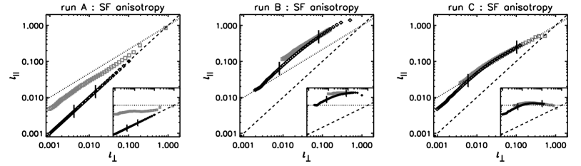
Figure 1.— Anisotropy of II-order structure functions $\ell_{\bot}(\ell_{||})$ obtained by identifying the scales at which parallel and perpendicular II-order SF have the same level, $S_{||}\equiv S(\ell_{||},0)=S(0,\ell_{\bot})\equiv S_{\bot}$. Black diamonds and gray squares indicate the anisotropy with respect to the global or to the local mean-field respectively. The vertical bars bound inertial range scales for the global SF as determined by the III-order SF (see text). The two reference straight lines indicate scale-independent anisotropy ($\ell_{||}=\ell_{\bot}$, dashed line) and the critical balance scale-dependent anisotropy ($\ell_{||}=\ell_{\bot}^{2/3}$, dotted line). From left to right, run A (isotropic, decaying turbulence), run B (anisotropic, forced, strong turbulence) and run C (anisotropic, forced, weak turbulence). Insets display the same plots compensated by $\ell_{\bot}^{2/3}$.

3. Simulations and numerical method.

We consider three high-resolution simulations of MHD turbulence whose parameters are listed in table 1. Run A is a developed decaying simulation of incompressible MHD turbulence without mean-field, representing isotropic turbulence. Run B is a simulation of weakly compressible MHD turbulence, with mean-field $B_{0}=5$ and anisotropic forcing. The forcing is applied only to components perpendicular to the mean-field and to wavevectors mainly perpendicular to the mean-field. Thus we are dealing with strong anisotropic turbulence of fluctuations with shear-Alfvén polarizations, a configuration akin to Reduced MHD. Finally run C is a simulation of incompressible MHD, again with mean-field $B_{0}=5$, but with a forcing which is isotropic in both components and wavevectors. In the latter the forcing is actually a freezing of the modes $1\leq k\leq 2$ that maintains an equal amount of pseudo-Alfvén and shear-Alfvén polarizations at large scales, along with equipartition between magnetic and kinetic energy and between Elsässer energies. This simulation can be classified as a case of weak anisotropic turbulence in terms of the strength parameter $\chi$ (see table 1), although it does not have the properties of classical weak turbulence (Ng & Bhattacharjee, 1997; Galtier et al., 2000; Meyrand et al., 2014). Indeed, the 3D spectrum has a relatively strong excitation in the parallel direction, resulting in a peculiar anisotropy $E(k,\theta)=A(\theta)k^{p}$, with an isotropic spectral index $p=-2-3/2$ in all directions (corresponding to a 1D spectrum with slope $-3/2$) and all the anisotropy appearing as a power anisotropy at large scales $A(\theta)$. We will not discuss the properties and the origin of such a spectrum that can be found in Müller & Grappin (2005); Grappin & Müller (2010); Grappin et al. (2013)); what is mostly relevant for the present analysis is that run C has a different 3D anisotropy compared to run B, although in both runs energy resides mainly in perpendicular wavevectors.

We will use three measures to characterize the simulations: II-order structure functions computed in the frame defined by the local mean-field (local $S$), II and III order structure functions, respectively $S$ and ${\boldsymbol{Y}}$, computed in an absolute frame attached to the $x$-axis, which is the direction of the global mean-field when it is present. For all structure functions, computation is made calculating increments in real space. Local $S$ are obtained following method I of (Cho & Vishniac, 2000), i.e. the local field at scale ${\boldsymbol{\ell}}$ is defined as ${\boldsymbol{B_{0}^{\ell}}}({\boldsymbol{x}})=1/2[{\boldsymbol{b}}({\boldsymbol{x}}+{\boldsymbol{\ell}})+{\boldsymbol{b}}({\boldsymbol{x}})]$. Note that the measure of anisotropy, i.e. the ratio $S(\ell_{\bot},0)/S(0,\ell_{||})$ of local $S$, is not unambiguously defined. In a turbulent medium fluctuations have a wide range of excited scales and the definition of the mean field depends on both scale and position. Thus, higher-order statistics may be introduced in the local $S$ to a different extent, depending on the averaging procedure. However, the two-point average employed in this work is a good working definition, at least in simulations of homogeneous turbulence since it was shown to yield the same results as line average or volume averages, provided that the averaging scale is smaller than the correlation length (Matthaeus et al., 2012). The computation of local $S$ is made for the whole range of available increments ${\boldsymbol{\ell}}$ but the average is made on a subset of grid points (typically $N_{x}\times N_{y}\times N_{z}=32^{3}$), which was checked to be a sufficient statistics for the anisotropy to converge. On the other hand the III-order structure functions ${\boldsymbol{Y}}$ are signed quantities and their computation requires large statistics to converge. Thus given the number of grid points $N$ in a given direction, we compute ${\boldsymbol{Y}}$ either on a smaller range of increments ($\ell=(1...N/M)dx$ with typically $M=4$, $dx$ is the grid size), or on a coarser grid of increments ($\ell=(1...N/M)Mdx$, with typically $M=4$), but still on all the grid points, so the averages are made on a sample of $\gtrsim 10^{7}$ data. The dissipation rate ($\epsilon$) entering the KHYPP equation (2) is obtained directly from the 3D Fourier spectra of magnetic and velocity field ($\hat{b}$ and $\hat{u}$ respectively),

$$\epsilon=-\partial_{t}E=\nu\Sigma_{k}k^{2}\hat{u}^{2}_{k}+\eta\Sigma_{k}k^{2}\hat{b}^{2}_{k}.$$ (10)

The terms appearing in Equation (2) are evaluated for four consecutive snapshots separated by approximately a nonlinear time (for the time derivative $\partial_{t}S$ we use a simple first-order scheme). All quantities entering the KHYPP equation are normalized to the dissipation rate $\epsilon$ and then averaged over the four snapshots. The 3D data are finally reduced for purposes of representation and analysis by performing an isotropization (averaging over polar and azimuthal angle $\theta$ and $\phi$ in spherical coordinates),

$$\left.\boldsymbol{\nabla}\cdot{\boldsymbol{Y}}\right|_{iso}=\frac{1}{4\pi}\int\left(\frac{\partial{Y_{x}}}{\partial{\ell_{x}}}+\frac{\partial{Y_{y}}}{\partial{\ell_{y}}}+\frac{\partial{Y_{z}}}{\partial{\ell_{z}}}\right)\mathrm{sin}\theta\mathrm{d}\phi\mathrm{d}\theta,$$ (11)

or an axisymmetrization (averaging over the azimuthal angle $\phi$ in cylindrical coordinate with axis along the $\ell_{x}$),

$$\left.\boldsymbol{\nabla}\cdot{\boldsymbol{Y}}\right|_{axis}=\frac{1}{2\pi}\int\left(\frac{\partial{Y_{x}}}{\partial{\ell_{x}}}+\frac{\partial{Y_{y}}}{\partial{\ell_{y}}}+\frac{\partial{Y_{z}}}{\partial{\ell_{z}}}\right)\mathrm{d}\phi.$$ (12)

In the following we drop the subscripts $iso$ and $axis$ and eventually mention explicitly the average procedure used for representation.

4. Results

4.1. Anisotropy of II-order structure functions

We measured the anisotropy of II-order SF in two frames. In the global frame the increments $\ell_{||}$ and $\ell_{\bot}$ are taken parallel and perpendicular to a fixed direction $x$, which is the direction of the mean-field ${\boldsymbol{B_{0}}}$ when it is present. In the local frame the parallel and perpendicular directions are relative to the scale-dependent mean-field direction ${\boldsymbol{B_{0}^{\ell}}}$ (see section 2). The measure of the anisotropy is obtained by identifying the couples of increments ($\ell_{||},~{}\ell_{\bot}$) at which the parallel and the perpendicular SF have the same value: $S_{||}\equiv S(\ell_{||},~{}0)=S_{\bot}\equiv S(0,~{}\ell_{\bot})$, i.e. the function $\ell_{||}(\ell_{\bot})$ measures the aspect ratio of isolevels of the SF at different scales, also known as eddy shape. Scale-independent anisotropy results in a linear relation $\ell_{||}\propto\ell_{\bot}$, that is, an aspect ratio $\ell_{\bot}/\ell_{||}$ that does not change with scale. Conversely, scale-dependent anisotropy results in a deviation from the linear scaling $\ell_{||}\propto\ell_{\bot}^{p}$, with $p<1$: the aspect ratio of SF, $\ell_{\bot}/\ell_{||}$ increases at smaller scales, that is, eddies become more and more elongated in the parallel direction. In figure 1 we plot $\ell_{||}(\ell_{\bot})$ for the two measures of anisotropy, local (gray squares) and global (black diamonds), for the three runs listed in table 1. The dashed line, with slope $-1$, is a reference for scale-independent anisotropy. The dotted line is a reference for the scale-dependent anisotropy predicted by the critical balance relation (Goldreich & Sridhar, 1995):

$$\ell_{||}\propto\ell_{\bot}^{2/3}.$$ (13)

The insets display the same plots compensated by the critical balance anisotropy in order to better appreciate the scaling relation $\ell_{||}(\ell_{\bot})$.

In the local frame, all runs have a scale-dependent anisotropy extending to a wide range of scales. The function $\ell_{||}(\ell_{\bot})$ has a slope flatter than $1$, thus the anisotropy grows with decreasing scales and eddies are more and more elongated in the parallel direction. The scaling law actually follows the critical balance anisotropy Equation (13) in the range where $S_{\bot}\propto\ell_{\bot}^{2/3}$, extending for about a decade for runs A, B, and C in the intervals $0.008\lesssim\ell_{\bot}\lesssim 0.05$, $0.02\lesssim\ell_{\bot}\lesssim 0.2$, and $0.008\lesssim\ell_{\bot}\lesssim 0.08$ respectively. This critical balance anisotropy is quite robust since in all runs the anisotropic relation holds rather well even outside the above-mentioned range of scales where $S_{||}$ and $S_{\bot}$ have a clear power-law scaling. Note that run C is a weak turbulence simulation, and it is not obvious that it should have a critical balance anisotropy (see Galtier et al. 2005 for an explanation based on a heuristic model of anisotropic turbulence).

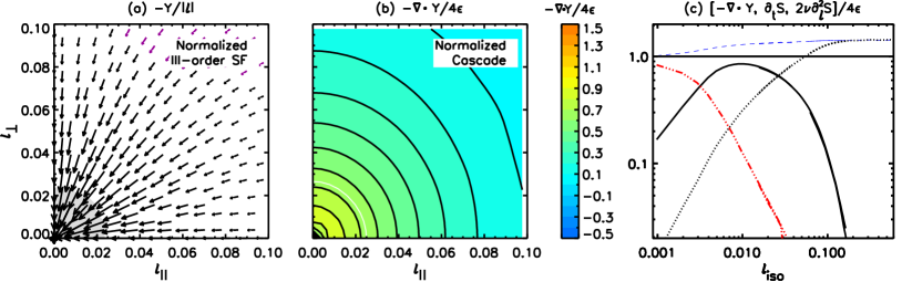
Figure 2.— Run A, $B_{0}=0$, isotropic decaying turbulence. Panel (a). III-order structure function, or Yaglom flux ${\boldsymbol{Y}}$, projected on the ($\ell_{||},~{}\ell_{\bot}$) plane and normalized by the scalar increment $\ell$. Arrows are colored according to their angle $\theta_{R}$ with respect to the radial direction (black is for $0^{o}\leq\theta_{R}<5^{o}$, violet is for $\theta_{R}\geq 5^{o}$), their length is proportional to $|{\boldsymbol{Y}}|/\ell$. Panel (b). Isocontour of $-\boldsymbol{\nabla}\cdot{\boldsymbol{Y}}$ normalized by the dissipation rate $4\epsilon$. Panel (c). Comparison of different terms appearing in the KHYPP equation, Equation (2), after isotropization and normalization by $4\epsilon$: the divergence of the Yaglom flux $-\boldsymbol{\nabla}\cdot{\boldsymbol{Y}}$ (black solid line), the time dependent term $\partial_{t}S$ (dotted black line), the dissipative term $2\nu\partial_{l}^{2}S$ (red triple-dot-dashed line), and the sum of the three terms (long-dashed blue line). The thick solid horizontal line is a reference for $4\epsilon$. The gray area in panel (a) and the white thick lines in panel (b) bound the scales at which $-\boldsymbol{\nabla}\cdot{\boldsymbol{Y}}$ is larger than the other terms in the KHYPP equation, it is a rough estimate of inertial range scales.

Consider now the anisotropy measured in the global frame (black diamonds in Figure 1), which will be more relevant for the following analysis, since it is related to the III-order SF by the KHYPP equation (2). As expected, run A is perfectly isotropic, the aspect ratio is unity at all scales. The anisotropy of strong turbulence, run B, becomes scale-independent (it has a slope equal to one) for scales $\ell_{\bot}\lesssim 0.08$, approaching a constant ratio $\ell_{||}/\ell_{\bot}=A\approx 10$ at small scales. For weak turbulence, run C, the anisotropy becomes scale-independent only at very small scales ($\ell_{\bot}\lesssim 0.01$), with an aspect ratio $A\approx 5$ that is smaller compared to strong turbulence. The vertical bars in the plot bound the inertial range as identified from Equation (3) . While run B has a scale-independent anisotropy that develops in the inertial range, in run C scale-independent anisotropy is attained only at dissipative scales. Thus, at inertial-range scales the anisotropy is mostly scale dependent in our weak turbulence simulation (run C): it follows the critical balance scaling $\ell_{||}\propto\ell_{\bot}^{2/3}$ even when measured in the global frame, contrary to expectations (Chen et al., 2011).

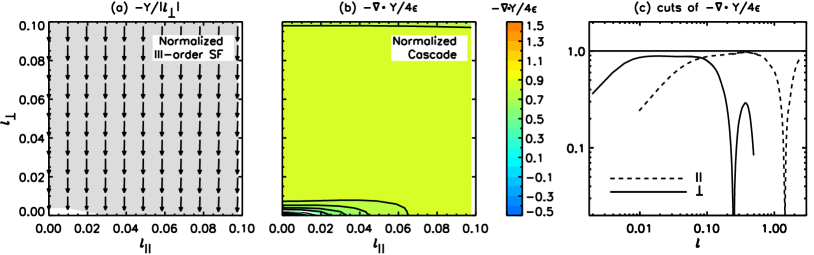
Figure 3.— Run B, $B_{0}=5$, strong turbulence. Panel (a). III-order structure function, or Yaglom flux ${\boldsymbol{Y}}$, projected on the ($\ell_{||},~{}\ell_{\bot}$) plane and normalized by the perpendicular increment $\ell_{\bot}$. Arrows are colored according to their angle $\theta_{\bot}$ with respect to the perpendicular direction direction (black is for $0^{o}\leq\theta_{\bot}<5^{o}$), their length is proportional to $|{\boldsymbol{Y}}|/\ell_{\bot}$. Panel (b). Isocontour of $-\boldsymbol{\nabla}\cdot{\boldsymbol{Y}}$ normalized by the dissipation rate $4\epsilon$. Panel (c). Cuts of $-\boldsymbol{\nabla}\cdot{\boldsymbol{Y}}$ in directions parallel (dashed line) and perpendicular (solid line) to the mean-field $B_{0}$. The thick solid horizontal line is a reference for $4\epsilon$. The gray area in panel (a) and the white thick lines in panel (b) bound the scales at which $-\boldsymbol{\nabla}\cdot{\boldsymbol{Y}}$ is larger than the other terms in the KHYPP equation, it is a rough estimate of inertial range scales.

4.2. III-order structure functions and KHYPP equation

4.2.1 Isotropic case

We consider first the isotropic case (run A) for which $S$ is isotropic, so we expect also to find an isotropic III-order SF. In Figure 3, panel (a), we plot the Yaglom flux ${\boldsymbol{Y}}$ (III-order SF), averaged along the polar angle of cylindrical coordinates with axis $\ell_{x}\equiv\ell_{||}$, and normalized by the scalar increment $\ell$. We consider relatively small scales (the largest scale is $\ell=0.5$) to highlight inertial range features, as will be clearer below. The Yaglom flux is almost radial at large scales and becomes remarkably radial at smaller scales $\ell\lesssim 0.08$. The length of the arrows increases toward the origin, indicating that the intensity of the cascade increases when approaching the inertial range (the gray area) while keeping the same (radial) direction. Note also that the arrow length is constant on circles of given $\ell$, meaning that ${\boldsymbol{Y}}\approx\mathrm{Const}\times{\boldsymbol{\ell}}$ as expected for isotropic turbulence, Equation (6).

In panel (b) we plot the isocontours of the divergence of the Yaglom flux, normalized by the dissipation rate. The isocontours are roughly isotropic at large scales and become perfectly isotropic at small scales ($\ell\leq 0.03$). In a small interval of scales around $\ell\approx 0.01$, the divergence $-\boldsymbol{\nabla}\cdot{\boldsymbol{Y}}$ has a maximum reaching the value $\approx 0.9$. Thus, the dissipation rate is approximately equal to the cascade rate, and these scales can be identified as the inertial range of turbulence. However, the divergence is not strictly a constant, as expected for the inertial range. Note that although the latter is very short, it is uniformly distributed among scales.

Finally, in panel (c) we plot in logarithmic scales, after isotropization and normalization by $4\epsilon$, all the terms appearing in the KHYPP equation, Equation (2), namely, the divergence of the Yaglom flux $-\boldsymbol{\nabla}\cdot{\boldsymbol{Y}}$ (thick solid line), the dissipative term $2\nu\partial_{\ell}^{2}S$ (red triple-dot-dashed line), and the time-dependent term $\partial_{t}S$ (dotted line). The dissipative term dominates at small scales, while the time-dependent term (decay) dominates at large scales. The cascade term, $-\boldsymbol{\nabla}\cdot{\boldsymbol{Y}}$, is larger than the other terms for scales $0.003\lesssim\ell\lesssim 0.03$ (the gray area in panel (a)). These two extrema can be identified with the injection scale and the dissipative scale, respectively. It is worth noting that the dissipation scale defined in this way coincides with the estimate based on II-order SF in Figure 1. From this logarithmic plot it is clear that the inertial range is quite small in this decaying simulation because $-\boldsymbol{\nabla}\cdot{\boldsymbol{Y}}$ is much larger than other terms only in a small interval centered at $\ell\approx 0.01$, where it is roughly horizontal and equal to 0.9 (it should be equal to one in an ideally infinite inertial range).

In the same plot we also traced, as a blue long-dashed line, the sum of the three terms just discussed, that should amount at all scales to the dissipation rate $4\epsilon$ (thick solid horizontal line) for good energy conservation. The sum is an almost horizontal straight line, only a factor $1.2$ higher than the dissipation rate for scales $\ell\gtrsim 0.005$. This confirms that the statistics is large enough to ensure convergence and that the conservation of energy holds with sufficient accuracy except at very small scales where a small numerical dissipation probably kicks in: the injection at large scale (including the decay), the cascade in the inertial range, and the dissipation at small scales all occur at the same rate.

To summarize, the analysis of the isotropic turbulence confirms the theoretical expectations: inside the inertial range the Yaglom flux is radially directed and its magnitude scales linearly with the scalar increment $\ell$. The divergence of the Yaglom flux is approximately constant in the inertial range, and it is uniformly distributed among scales (isotropic). Note, however, that the extent of the inertial range is very limited due to the relatively small Reynolds number that prevents the formation of a large range of scales where the divergence of the Yaglom flux is the dominant term. With the current resolution ($1024^{3}$) it is at best half a decade, indicating that this is the minimal resolution required for studies of decaying turbulence (although hyperviscosity would probably alleviate the problem). This is relevant for solar wind studies (Dong et al., 2014), in which expansion induces an additional decay of magnetic and kinetic energy on top of the decay due to the turbulent dissipation.

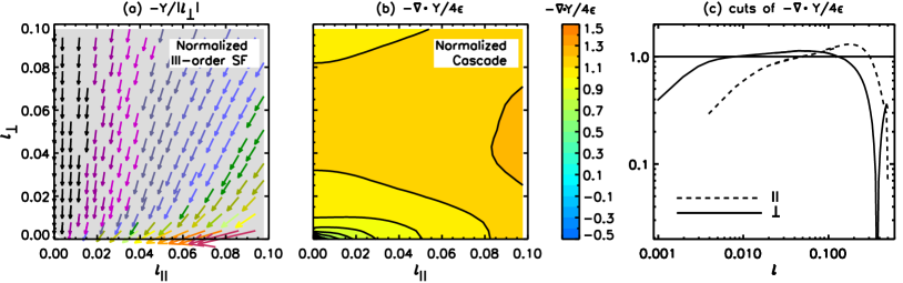
Figure 4.— Run C, $B_{0}=5$, weak turbulence. Same as in Figure 3. In panel (a) the arrow colors, from black to purple, indicate $\theta_{\bot}\in[0^{o},90^{o}]$ binned in intervals of $5^{o}$.

4.2.2 Anisotropic case, strong turbulence

Let’s now turn to the anisotropic run B, which is a simulation of strong turbulence with guide field and forced at large scales on components perpendicular $B_{0}$. In Figure 3, panel (a) we plot again the III-order SF, i.e. the Yaglom flux ${\boldsymbol{Y}}$, averaged over the polar angle in cylindrical coordinates with axis along increments parallel to the mean magnetic field. At variance with the isotropic case, the arrows are colored according to the angle $\theta_{\bot}$ formed with respect to the perpendicular direction (black color stands for $\theta_{\bot}\leq 5^{o}$), and their length is normalized to the perpendicular increment $\ell_{\bot}=(\ell_{y}^{2}+\ell_{z}^{2})^{1/2}$. The Yaglom flux is remarkably vertical in the inertial range (the gray area), and it is proportional to the perpendicular increments ${\boldsymbol{Y}}\propto{\boldsymbol{\ell_{\bot}}}$ (the arrow length is uniform in the whole inertial range, after normalization). This suggest that turbulence is undergoing a purely 2D cascade, Equation (8).

In panel (b) the normalized divergence of the Yaglom flux is constant over a large interval of parallel and perpendicular increments, with a value close to 1 (the light-green area at level $0.9$). However it is not uniformly distributed among scales, the isocontour of constant divergence extends to smaller perpendicular scales, suggesting that the cascade is not removing positive correlation from the parallel direction. This is consistent with Figure 1b that shows a clear anisotropy of $S$ in favor of a two-dimensionalization in the perpendicular plane.

This can be better appreciated in panel (c), where we plot cuts along the parallel and perpendicular directions of the divergence of the Yaglom flux in logarithmic scales. There is a very nice constant divergence in the perpendicular direction, with a value close to the dissipation rate (the horizontal thick solid line at level 1), covering about one decade in the range $0.01\lesssim\ell_{\bot}\lesssim 0.1$. In the parallel direction, an approximate inertial range is also found, having a smaller extent and shifted to larger scales $0.1\lesssim\ell_{||}\lesssim 0.6$.

We recall that from $-\boldsymbol{\nabla}\cdot{\boldsymbol{Y}}$ (panels (b) and (c)) one can identify the location of the inertial range and its distribution among parallel and perpendicular scales. On the other hand, the simple dependence of the Yaglom flux allows us to identify the cascade as a 2D cascade with ${\boldsymbol{Y}}=-2\epsilon{\boldsymbol{\ell_{\bot}}}$ We anticipate that ${\boldsymbol{Y^{\mp}}}=\left\langle\Delta{\boldsymbol{z^{\pm}}}|\Delta{\boldsymbol{z^{\mp}}}|^{2}\right\rangle$ have only perpendicular components because there is a dominance of shear-Alfvén polarizations. Indeed, these polarizations have $\Delta{\boldsymbol{z^{\pm}}}$ lying in the perpendicular plane and, as a consequence, the cascade is 2D. This simple picture of 2D cascade does not hold anymore as soon as pseudo polarizations, which have out-of-plane components, are energetically important.

4.2.3 Anisotropic case, weak turbulence

We finally consider the case of weak turbulence with guide field (run C), which is forced isotropically at small wavevectors $1\leq|{\boldsymbol{k}}|\leq 2$ by imposing at all times (freezing) the corresponding Fourier modes of the fluctuating fields ${\boldsymbol{B}},~{}{\boldsymbol{u}}$ (note that their $x,y,z$ components have also equal energy). In fig.4, panel (a) one can see immediately that the Yaglom flux is oblique, with an angle $\theta_{\bot}$ that changes with scales (we normalize arrow length by the perpendicular increment $|{\boldsymbol{Y}}|/\ell_{\bot}$ as in Figure 3). This means that the III-order SF has a parallel component and a non-negligible dependence on the parallel increments, thus contributing to the cascade rate through the divergence of the Yaglom flux. Such contribution seems to decrease at small parallel scales, where the Yaglom flux becomes vertical, hinting to a milder two-dimensionalization of this weak turbulence cascade.

Isocontours of $-\boldsymbol{\nabla}\cdot{\boldsymbol{Y}}$ are plotted in panel (b), with the usual normalization by $4\epsilon$. The inertial range can be identified with the light-orange area at level $1.1$, extending to a wide range of parallel and perpendicular scales. Its distribution is non-uniform and more complex than that of strong turbulence (Figure 3b), reflecting the dependence of the III-order SF from $\ell_{\bot}$ and $\ell_{||}$.

Panel (c) shows cuts of the divergence of the Yaglom flux along the parallel and perpendicular directions. Although the divergence is not exactly constant, the inertial range covers more than one decade in the perpendicular direction, $0.005\lesssim\ell_{\bot}\lesssim 0.1$, yielding a cascade rate that is slightly higher than the dissipation rate $4\epsilon$. On the other hand, the cut in the parallel direction is less flat, making more questionable the identification of an inertial range in this direction. The approximate parallel inertial range is shorter and located at larger scales, $0.03\lesssim\ell_{||}\lesssim 0.3$.

4.2.4 The KHYPP equation for pseudo and shear Alfvén polarizations

Decomposing fluctuations in pseudo and shear Alfvén polarizations proves useful to analyze in some more detail the relation between the Yaglom flux and the cascade rate in run C, which is a simulation of incompressible MHD. The decomposition is made in Fourier space, where pseudo Alfvén polarizations and shear Alfvén polarizations are oriented along the unitary vectors (e.g. Maron & Goldreich 2001),

$${\boldsymbol{\xi_{sh}}}=\frac{{\boldsymbol{k}}\times{\boldsymbol{B_{0}}}}{[1-({\boldsymbol{k}}\cdot{\boldsymbol{B_{0}}})^{2}]^{1/2}},\;\;\;\;{\boldsymbol{\xi_{ps}}}=\frac{{\boldsymbol{B_{0}}}-({\boldsymbol{k}}\cdot{\boldsymbol{B_{0}}}){\boldsymbol{k}}}{[1-({\boldsymbol{k}}\cdot{\boldsymbol{B_{0}}})^{2}]^{1/2}}.$$ (14)

This decomposition is completely equivalent to the decomposition into toroidal and poloidal components of the magnetic fluctuations. In incompressible MHD the same decomposition applies to the velocity field, which is also solenoidal. Shear Alfvén polarizations are the proper Alfvén modes in full MHD. Their component is perpendicular to both the mean field ${\boldsymbol{B_{0}}}$ and the wavevector ${\boldsymbol{k}}$, being incompressible. The pseudo Alfvén polarizations are the incompressible limit of slow modes in MHD. Their component lies in the plane identified by the mean field and the wavevector, and it is again perpendicular to the wavevector. For fluctuations with strong anisotropic spectra ($k_{\bot}>>k_{||}$), shear polarizations have wavevectors and components lying in the plane perpendicular to $B_{0}$, thus they represent the 2D modes in the slab-plus-2D decomposition introduced by Matthaeus et al. (1990). Instead, pseudo polarizations have wavevectors in the plane perpendicular to $B_{0}$ but components along $B_{0}$. This polarization, which is absent in Reduced MHD, is instead present in 2.5D configurations with out-of-plane mean field, and should not be confused with the slab component that has wavevectors parallel to $B_{0}$ and fluctuations perpendicular to it (and is thus included in Reduced MHD).

After decomposing fluctuations in pseudo and shear Alfvén polarizations, we go back to the real space and compute separately all the contributions to the KHYPP equation, Equation (2). Note that for strictly parallel wavevectors the pseudo-shear decomposition degenerates, so we remove such modes (the slab component) in the following analysis to avoid arbitrary partition of energy into the shear and pseudo polarizations. Using Parseval’s theorem $\langle\Delta{\boldsymbol{z^{\pm}_{ps}}}\cdot\Delta{\boldsymbol{z^{\pm}_{sh}}}\rangle=0$, the decomposed KHYPP equation can be written as:

$$\partial_{t} (S_{sh}+S_{ps})-2\nu\boldsymbol{\nabla}^{2}_{\ell}(S_{sh}+S_{ps})+4\epsilon=$$ (15)

$$- \boldsymbol{\nabla}_{\ell}\cdot\left\langle\Delta{\boldsymbol{z_{sh}}}|\Delta{\boldsymbol{z_{sh}}}|^{2}+\Delta{\boldsymbol{z_{sh}}}|\Delta{\boldsymbol{z_{ps}}}|^{2}\right\rangle$$ (16)

$$- \boldsymbol{\nabla}_{\ell}\cdot\left\langle\Delta{\boldsymbol{z_{ps}}}|\Delta{\boldsymbol{z_{sh}}}|^{2}+\Delta{\boldsymbol{z_{ps}}}|\Delta{\boldsymbol{z_{ps}}}|^{2}\right\rangle$$ (17)

$$- \boldsymbol{\nabla}_{\ell}\cdot\left\langle 2\Delta{\boldsymbol{z_{sh}}}(\Delta{\boldsymbol{z_{sh}}}\cdot\Delta{\boldsymbol{z_{ps}}})+2\Delta{\boldsymbol{z_{ps}}}(\Delta{\boldsymbol{z_{sh}}}\cdot\Delta{\boldsymbol{z_{ps}}})\right\rangle,$$ (18)

where we summed the $\pm$ species and dropped $\pm$ superscripts, i.e. $S_{sh}=1/2\langle|\Delta{\boldsymbol{z^{+}_{sh}}}|^{2}+|\Delta{\boldsymbol{z^{-}_{sh}}}|^{2}\rangle$, $\Delta{\boldsymbol{z_{sh}}}|\Delta{\boldsymbol{z_{ps}}}|^{2}=1/2[\Delta{\boldsymbol{z^{+}_{sh}}}|\Delta{\boldsymbol{z^{-}_{ps}}}|^{2}+\Delta{\boldsymbol{z^{-}_{sh}}}|\Delta{\boldsymbol{z^{+}_{ps}}}|^{2}]$, etc …

The III-order SF on the rhs is split into three lines containing respectively (1) the strain of the shear polarizations on the shear and pseudo energies, (2) the strain of the pseudo polarizations on the shear and pseudo energies, and (3) the mixed terms accounting for the exchange of energy during the cascade between the shear and pseudo polarizations. We anticipate that the mixed terms are negligible in the inertial range, thus we split the above equation into a system of equations for $S_{ps}$ and $S_{sh}$, with their own cascade rate $\epsilon_{sh}$ and $\epsilon_{ps}$,

$$\partial_{t}S_{sh}-2\nu\boldsymbol{\nabla}^{2}_{\ell}S_{sh}+4\epsilon_{sh}=-\boldsymbol{\nabla}_{\ell}\cdot\left\langle\Delta{\boldsymbol{z_{sh}}}|\Delta{\boldsymbol{z_{sh}}}|^{2}+\Delta{\boldsymbol{z_{ps}}}|\Delta{\boldsymbol{z_{sh}}}|^{2}\right\rangle,$$

(19)

$$\partial_{t}S_{ps}-2\nu\boldsymbol{\nabla}^{2}_{\ell}S_{ps}+4\epsilon_{ps}=-\boldsymbol{\nabla}_{\ell}\cdot\left\langle\Delta{\boldsymbol{z_{sh}}}|\Delta{\boldsymbol{z_{ps}}}|^{2}+\Delta{\boldsymbol{z_{ps}}}|\Delta{\boldsymbol{z_{ps}}}|^{2}\right\rangle.$$

(20)

Note that each equation contains only quadratic terms of a given Alfvén polarization (shear or pseudo) even in the III-order SF. On the rhs of Equations (19)-(20), the second terms represent an active contribution to the cascade of pseudo Alfvén polarizations: if it is vanishing or negligible the pseudo Alfvén polarizations can be said passive.

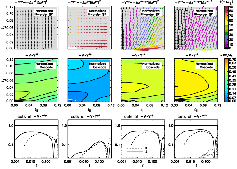
Figure 5.— Run C. Decomposition of the KHYPP equation for shear and pseudo energies. As in figs. 3, 4, ${\boldsymbol{Y}}$ is normalized by $\ell_{\bot}$, $-\boldsymbol{\nabla}\cdot{\boldsymbol{Y}}$ is normalized by $4\epsilon$. In the first three columns we analyze the KHYPP equation for pseudo energy, Equation (20), by plotting the contribution to the cascade appearing on the rhs of Equation (20). The first term, i.e. the strain of shear polarizations on the pseudo energy (column 1); the second term, i.e. the strain of pseudo polarizations on pseudo energy (column 2); and their sum (column 3). In column 4 we consider the cascade for shear energy, Equation (19), without separating the pseudo and shear contribution. In the bottom panel, fourth column, we also plot with grey color the contribution of the mixed terms, Equation (18).

This separation will appear justified by the analysis of each term, which is presented in Figure 5 in the same format of figs. 3, 4, i.e. with the the Yaglom flux normalized by the perpendicular increment, ${\boldsymbol{Y}}/\ell_{\bot}$, and the divergence normalized by the cascade rate, $-\boldsymbol{\nabla}\cdot{\boldsymbol{Y}}/4\epsilon$. We consider separately the two contributions in the rhs terms of the equation for the pseudo energies, Equation (20). In the first column we have the III-order SF accounting for the strain of shear polarizations acting on the pseudo energy, ${\boldsymbol{Y}}^{\mathrm{SP}}=\left\langle\Delta{\boldsymbol{z_{sh}}}|\Delta{\boldsymbol{z_{ps}}}|^{2}\right\rangle$ (the first term in the rhs). The Yaglom flux (upper panel) is perpendicular, as in run B, since the vectorial part of ${\boldsymbol{Y}}^{\mathrm{SP}}$ is made of only shear polarizations, which have only perpendicular components. Its magnitude depends mostly on $\ell_{\bot}$ as can be guessed by the length of the arrows, with a small dependence on $\ell_{||}$ at large parallel scales. This dependence is better appreciated on the map of $-\boldsymbol{\nabla}\cdot{\boldsymbol{Y}}^{\mathrm{SP}}$ (middle panel) that has slightly inclined isocontours instead of horizontal isocontours. The inertial range identified with the green area at level $\approx 0.4$ is non uniformly distributed in the $(\ell_{||},~{}\ell_{\bot})$ plane, occupying preferentially perpendicular scales $\ell_{\bot}<0.05$ independently of parallel scale. In the bottom panel one can better locate the inertial range which is much more extended toward smaller scales in the perpendicular than in the parallel direction.

In the second column, we analyze the III-order SF accounting for the strain of pseudo polarizations on the pseudo energy, ${\boldsymbol{Y}}^{\mathrm{PP}}=\left\langle\Delta{\boldsymbol{z_{ps}}}|\Delta{\boldsymbol{z_{ps}}}|^{2}\right\rangle$, the second term in the rhs of Equation (20). Note that the Yaglom flux is now horizontal (excepts at small parallel scales $\ell_{||}\lesssim 0.03$), since for a spectrum (or II-order SF) with energy residing mainly in perpendicular wavevectors, pseudo polarizations have a dominant parallel component. The contribution to the divergence (middle panel) is almost complementary to the previous term, being larger at large parallel and perpendicular scales while it is negligible in the inertial range. This is better seen in the bottom panel, in which it is also shown clearly that this III-order SF does not form an inertial range on its own, but it is responsible for a non-constant energy flux from large to small scales in both parallel and perpendicular directions. One would be tempted to model the two terms, ${\boldsymbol{Y}}^{\mathrm{SP}}$ and ${\boldsymbol{Y}}^{\mathrm{PP}}$, as 2D+1D components respectively, according to the orientation of the Yaglom flux. However, such a decomposition does not work since the candidate for the 1D component (${\boldsymbol{Y}}^{\mathrm{PP}}$) has a strong dependence on $\ell_{\bot}$ (second column, top panel), and its divergence does not yield any identifiable inertial range (second column, middle and bottom panels).

Finally in the third column we analyze the sum of the two terms just discussed, ${\boldsymbol{Y}}^{\mathrm{*P}}={\boldsymbol{Y}}^{\mathrm{PP}}+{\boldsymbol{Y}}^{\mathrm{SP}}=\left\langle(\Delta{\boldsymbol{z_{sh}}}+\Delta{\boldsymbol{z_{ps}}})|\Delta{\boldsymbol{z_{ps}}}|^{2}\right\rangle$, the whole rhs of Equation (20). The Yaglom flux is now oblique, with dependence on both $\ell_{\bot}$ and $\ell_{||}$, the latter being mostly inherited from the strain of pseudo polarizations (${\boldsymbol{Y}}^{\mathrm{PP}}$), indicating a smaller degree of two-dimensionalization for turbulence of pseudo Alfvén polarizations, compared to the strong turbulence of run B. In the middle panel the inertial range extends to parallel and perpendicular scales in a way somewhat similar to run B, although the Yaglom flux is quite different. Comparing the bottom panels in columns one, two, and three, one can see that the strain of both shear and pseudo polarizations contribute to the formation of the wide inertial range in the perpendicular direction $0.005\lesssim\ell_{\bot}\lesssim 0.1$, as well as to the shorter inertial range found at larger scales in the parallel direction $0.03\lesssim\ell_{\bot}\lesssim 0.2$ (their ranges coincide with those one obtained without separating shear and pseudo polarizations). More precisely, shear polarizations contribute with a constant cascade at small scales ($\ell\lesssim 0.04$), while pseudo polarizations control the injection of energy into the cascade at large scales ($\ell\approx 0.1$).

We do not repeat the analysis of the strain of shear and pseudo polarizations on shear energy, Equation (19), since it yields qualitatively similar results. The only noticeable difference is that the Yaglom flux ${\boldsymbol{Y}}^{\mathrm{PS}}=\left\langle\Delta{\boldsymbol{z^{ps}}}|\Delta{\boldsymbol{z^{sh}}}|^{2}\right\rangle$ is radially directed instead of being horizontal. We plot in the fourth column the whole contribution to the cascade of shear energy, ${\boldsymbol{Y}}^{\mathrm{*S}}=\left\langle(\Delta{\boldsymbol{z_{sh}}}+\Delta{\boldsymbol{z_{ps}}})|\Delta{\boldsymbol{z_{sh}}}|^{2}\right\rangle$. Comparing the third and fourth columns, one can see that (i) shear and pseudo energy cascade qualitatively in a similar way (top panels), although the Yaglom flux for shear polarizations, ${\boldsymbol{Y}}^{\mathrm{*S}}$, is more perpendicular (more 2D); (ii) the cascade rate is slightly stronger for shear energy than for pseudo energy (middle panels); and (iii) a clear inertial range is found for both shear and pseudo energies (bottom panel) following the decomposition of Equations (19)-(20).

In the fourth column, bottom panel, we also plot the sum of the mixing terms, Equation (18), along the parallel and perpendicular increments (gray lines). They are negligible compared to all other terms in the inertial range, indicating that the shear and pseudo polarizations cascade without exchanging their energy, as already pointed out by Maron & Goldreich (2001) for decaying simulations. However, at large scales $\ell\approx 0.2$, they are of the same order of the term accounting for the strain exerted by pseudo polarizations (II column, bottom panel in Figure 5), suggesting an exchange of energy between the shear and pseudo polarizations.

To summarize, in run C the freezing of large scales (forcing) causes an exchange of energy between pseudo and shear polarization at large scales. The two polarizations cascade in a similar manner (same rate, same inertial range) under the action (strain) of both the shear and pseudo polarizations. The flux toward small scales that is triggered by pseudo polarizations is smaller in magnitude and not constant (it is not a proper inertial range on its own), but it affects considerably the total cascade rate at large inertial-range scales ($\ell\approx 0.1$). On the other hand, the shear polarizations control the constant energy flux at small inertial-range scales ($\ell\lesssim 0.04$). Thus according to the separation made in Equations (19)-(20), the two cascades are not totally independent. Indeed, whatever the polarization considered ($S_{ps}$ or $S_{sh}$), the cascade is triggered by pseudo polarizations at the interface between injection scales and inertial range scales, while it is sustained by shear polarizations at smaller inertial range scales. The presence and importance of the pseudo polarizations is revealed by the Yaglom flux, the more pseudo polarizations are energetic, the more ${\boldsymbol{Y}}$ becomes oblique.

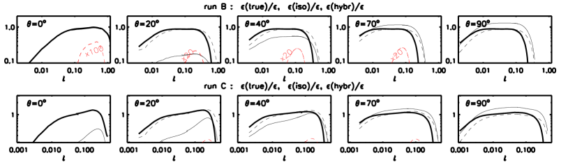
Figure 6.— Comparison of the true cascade rate, Equation (23) (solid thick line) with the isotropic cascade rate, Equation (21) (thin solid line), and the hybrid cascade rate, Equation (22) (dashed black line). The red dashed line is the 1D (parallel) cascade rate obtained within the hybrid method. From left to right, panels refer to increasing angles $\theta$ between the sampling direction ${\boldsymbol{\ell}}$ and the mean-field ${\boldsymbol{B_{0}}}$.

5. Anisotropy of the III-order SF and solar wind measurements

In measuring the cascade rate of solar wind turbulence through III-order SF, one needs to make assumptions on the unknown anisotropy of ${\boldsymbol{Y}}$. Despite the limitations due to the imposed symmetries, this brings the advantage of increasing the statistic, on the one hand, and of avoiding the computation of the divergence of ${\boldsymbol{Y}}$ on the other hand. Two common assumptions usually employed to reduce in-situ data will be tested against our anisotropic DNS (run B and C) in order to highlight possible systematic errors on the measure of the cascade rate in the solar wind.

The simplest assumption is that of isotropic turbulence, Equation (6), whose expression is repeated here for convenience,

$$\epsilon^{iso}=-\frac{3}{4}\frac{Y_{\ell}}{\ell},$$ (21)

and involves projecting ${\boldsymbol{Y}}$ along the direction of increments ($Y_{\ell}={\boldsymbol{Y}}\cdot{\boldsymbol{\ell}}/\ell$). As discussed in section 2, the cascade rate is directly obtained from the III-order SF without any need to compute derivatives. This “isotropic” method has been mainly employed for fast polar wind (Sorriso-Valvo et al., 2007; Marino et al., 2008, 2012) on Ulysses measurements.

Admitting some form of anisotropy, the minimal assumption is that of axisymmetry. To avoid computing derivatives along the two increments, one again resorts on simplified geometrical models, as the 2D+1D turbulence employed by Macbride et al. (2008); Stawarz et al. (2009, 2010) on WIND and ACE data in the ecliptic solar wind. This method assumes that the III-order SF has parallel and perpendicular components that depend only on the parallel and perpendicular increments, respectively (the cascade is independent in the two directions). The total cascade rate is obtained by combining the two independent equations for (isotropic) 2D-perpendicular and for 1D-parallel cascades (Equation (8) and Equation (9) respectively). Such a “hybrid” cascade rate reads

$$\epsilon^{hybr}=\epsilon^{1D}+\epsilon^{2D}=\epsilon^{||}+\epsilon^{\bot}=-\left(\frac{1}{4}\frac{Y_{||}}{\ell_{||}}+\frac{1}{2}\frac{Y_{\bot}}{\ell_{\bot}}\right).$$ (22)

The isotropic and hybrid cascades are obtained by first computing the 3D III-order SF, and then by applying the corresponding average (isotropy or axisymmetry). Similarly, the “true” cascade rate is obtained from Equation (12):

$$\epsilon^{true}=-\frac{1}{4}\frac{1}{2\pi}\int\left(\frac{\partial{Y_{x}}}{\partial{\ell_{x}}}+\frac{\partial{Y_{y}}}{\partial{\ell_{y}}}+\frac{\partial{Y_{z}}}{\partial{\ell_{z}}}\right)\mathrm{d}\phi.$$ (23)

We now compare in Figure 6 the true cascade rate (thick solid line) with the isotropic (thin solid line) and the hybrid (thin dashed line) cascade rate for run B and C (top and bottom panels, respectively). All cascade rates are normalized by the dissipation rate $\epsilon$ obtained directly from spectra, Equation (10). Each panel represents a cut in the $(\ell_{||},~{}\ell_{\bot})$ plane taken along a fixed direction that forms an angle $\theta$ with the mean-field direction.

The isotropic cascade rate is strongly angle dependent, independently of the run considered. It returns increasing cascade rates for increasing angles, as can be expected since both runs B and C have a dominant perpendicular cascade. It overestimates the true cascade rate at large angles ($\theta\gtrsim 70^{o}$) while it underestimates the true cascade rate by a factor $\approx 2$ even at $\theta=45^{o}$. The hybrid method instead performs very well: it does not vary with angle $\theta$ and yields the correct cascade rate at oblique angles $\theta\gtrsim 20^{o}$.

In the nearly parallel direction, both the hybrid and isotropic methods strongly underestimate the true cascade rate (by a factor $>10$) or they completely fail in yielding any cascade rate. Indeed, neither of the two methods is able to account for the dependence of the parallel component of the III-order SF on the perpendicular increments, ${\boldsymbol{Y_{||}}}(\ell_{\bot})$, which is instead fundamental in our strongly anisotropic runs (e.g. Figure 2a). Indeed, the 1D cascade entering the hybrid method is basically negligible at all angles (red dashed line in fig 6). This implies that the cascade is with a good approximation a 2D cascade in both our anisotropic runs. On the other hand, a linear scaling for the 1D cascade is found in the solar wind (e.g. Macbride et al. 2008), suggesting that the III-order SF of solar wind turbulence is less anisotropic than that one of runs B and C.

6. Summary and discussion

We studied the anisotropy of MHD turbulence with or without guide field ($B_{0}$) by means of structure functions (SF) of II and III order, in three direct numerical simulations of MHD turbulence at moderate and high resolution (see table 1). We consider isotropic decaying turbulence (run A), forced strong turbulence with mean-field (run B), and forced weak turbulence with mean-field (run C).

We used II-order SF ($S$) to characterize the anisotropy with respect to the local mean-field and to the global mean-field. The anisotropy with respect to the local mean-field is scale dependent in all runs (with or without mean-field) and follows the critical balance prediction $\ell_{||}\propto\ell_{\bot}^{2/3}$. This confirms previous theoretical and numerical findings (Goldreich & Sridhar, 1995; Cho & Vishniac, 2000; Maron & Goldreich, 2001), in the local frame the anisotropy grows at smaller and smaller scales. When instead we used as a reference the global mean-field, we found isotropy for MHD turbulence without mean-field (run A) and strong two-dimensionalization for turbulence with mean field, with run B being more anisotropic than run C (the small-scale aspect ratio is $\approx 10$ and $\approx 5$ respectively). Surprisingly, for run C, we found a scale-dependent anisotropy consistent with critical balance even when $S$ is computed in the frame attached to the mean field $B_{0}$, at variance with previous analysis in DNS (Chen et al., 2011) and in solar wind measurements (Tessein et al., 2009) which reported scale-independent anisotropy. A possible explanation is that run C has a strong magnetic field ($b_{rms}/B_{0}=1/5$) and so the local and global frames almost coincide. In favor of this explanation, the anisotropy becomes scale independent at smaller scales. However, there are other “non-standard” aspects of run C that could be related to scale-dependent anisotropy in the global frame: the special 3D spectrum that has an isotropic spectral slope but anisotropic energy levels in parallel and perpendicular direction (Grappin & Müller, 2010), the strong excitation of pseudo Alfvén polarizations (see below), and the isotropic forcing (freezing) that maintains a magnetic excess at large scales (Grappin et al., 2013). These three aspects could be all related to one another and are under investigation.

We then analyzed the vectorial III-order SF (or Yaglom flux, ${\boldsymbol{Y}}$), which is related to $S$ computed in the global frame by a generalization to incompressible MHD (Politano & Pouquet, 1998) of the Von Karman-Howart-Yaglom relation in hydrodynamics (KHYPP equation in the following). The III-order SF, ${\boldsymbol{Y}}$, is expected to be anisotropic for MHD turbulence with mean-field, but it has never been reported in DNS or experiments (except for rotating hydrodynamic turbulence experiments, Lamriben et al. 2011). Despite some anisotropic models exist (Podesta et al., 2007; Galtier, 2009, 2012), they have never been verified in DNS.

We tested the KHYPP equation in isotropic decaying turbulence (run A) and found that the Yaglom flux is almost purely radial, its divergence is isotropic, and the maximum of $-\boldsymbol{\nabla}\cdot{\boldsymbol{Y}}$ is of the order of the dissipation rate (only a factor 0.8 smaller), confirming theoretical expectations (Politano & Pouquet, 1998). However, the condition defining the inertial range, $-\boldsymbol{\nabla}\cdot{\boldsymbol{Y}}=const$, is only fairly satisfied in our decaying turbulence that has an inertial range of only half a decade despite the high resolution ($1024^{3}$). More interestingly, we showed that the familiar concept of Kolmogorov cascade in Fourier space also applies in the real space with SF. Note that no assumption on locality of nonlinear interactions is needed to obtain the KHYPP equation. Despite this, we found that injection, cascade, and dissipation occur at the same rate and that the cascade is achieved via a fairly constant nonlinear transfer in the inertial range. In particular, by comparing the divergence of the Yaglom flux with the other terms appearing in the KHYPP equation (dissipation term and decaying term), one can determine the dissipation scale and the injection scale of turbulence. This has important applications in solar wind turbulence, since, due to expansion, it is an intrinsically decaying turbulence for which the injection scale is not easily identified (Hellinger et al., 2013; Dong et al., 2014).

For strong turbulence with mean-field, we found that ${\boldsymbol{Y}}$ has only perpendicular components and depends only on perpendicular increments; this is a 2D turbulence as defined in Equation (7). The corresponding inertial range extends to small perpendicular scales, while it is shorter and located at larger scales in the parallel direction: the anisotropy of ${\boldsymbol{Y}}$ emerges as a non-uniform distribution of the scales having $-\boldsymbol{\nabla}\cdot{\boldsymbol{Y}}=const$. A similar non-uniform distribution is found in the forced, weak turbulence case (run C), with an important difference concerning the orientation of ${\boldsymbol{Y}}$. The latter is no more strictly perpendicular, but oblique. In particular, the Yaglom flux is almost radial at large parallel scales in the inertial range and becomes more and more perpendicular at small parallel scales. We interpret this behavior as a weaker two-dimensionalization of turbulence, since the oblique orientation of ${\boldsymbol{Y}}$ implies a dependence on parallel and perpendicular scales, in contrast to the purely 2D case in which ${\boldsymbol{Y}}={\boldsymbol{Y_{\bot}}}({\boldsymbol{\ell_{\bot}}})$.

By decomposing fluctuations into shear Alfvén and pseudo Alfvén polarizations in run C we also found that energetically important pseudo polarizations are responsible for the non-perpendicular III-order SF. The pseudo/shear decomposition allows us to prove that the two polarizations cascade independently, that is, without exchanging their energy, in the inertial range. One can thus write separate KHYPP equations for pseudo and shear energies. However, strictly speaking, the two cascades are not independent, since in each of them the strain of pseudo and shear polarizations enters the expression for the Yaglom flux. In particular the strain exerted by pseudo polarizations is associated with a non-constant cascade of energy at the large inertial-range scales; thus pseudo polarizations control the injection of energy in run C (although becoming passive at smaller inertial-range scales, e.g. Maron & Goldreich 2001; Cho & Lazarian 2003). In Grappin et al. (2013), it is shown how the equipartition of kinetic and magnetic energy at the large frozen scales is associated to the weaker anisotropy of the 3D spectrum of run C, having the property of a 3D Iroshnikov-Kraichnan turbulence. Here we argue that kinetic/magnetic equipartition at the largest scales induces an exchange of energy between pseudo and shear polarizations, thus allowing pseudo polarizations to control the cascade at the interface between injection and inertial-range scales.

Finally, on the anisotropic runs B and C we tested two methods that are commonly applied to obtain the cascade rate in the solar wind. The methods both rely on assumptions of the anisotropy of the III-order SF, allowing one to obtain the cascade rate directly from ${\boldsymbol{Y}}$ (i.e. without computing the divergence). The first method assumes that ${\boldsymbol{Y}}$ is isotropic. The second method (hybrid method) assumes axisymmetry and models the anisotropy as a geometric superposition of a 1D (parallel) cascade and an isotropic 2D (perpendicular) cascade. We found that the isotropic method is strongly angle dependent, yielding correct cascade rates only at large angles between the direction of increments and the magnetic field, translating to angles between the magnetic field direction and the solar wind direction $\theta_{BV}\gtrsim 70^{o}$ (needless to say, the isotropic method works very well for run A). For fast polar wind, emanating from stable coronal holes, turbulence is expected to have a strong anisotropy (Verdini et al., 2012; Perez & Chandran, 2013), comparable to our run B and C. We thus suggest that the angle dependence of the isotropic method is at the origin of the relatively small number of intervals ($13\%$) in which the linear scaling $Y_{\ell}\propto\ell$ is found in polar solar wind in-situ data (Marino et al., 2012). In contrast, the hybrid method performs very well on our anisotropic runs, yielding an angle-independent cascade rate for $\theta_{BV}\gtrsim 20^{o}$. Both methods fails to obtain any cascade rate when increments are parallel to the mean-field. This is due to the dependence ${\boldsymbol{Y_{||}}}(\ell_{\bot})$ that is excluded in both assumptions but present in all our runs. This, together with the good performance of the hybrid method, indicates that the anisotropic runs B and C are fairly well described by a 2D cascade model, despite their different degree of anisotropy. Note that in the solar wind a 1D cascade, actually a linear scaling $Y_{||}\propto\ell_{||}$, is indeed measured with the hybrid method, indicating that solar wind turbulence in the ecliptic has a different and probably much weaker anisotropy compared to our DNS.

We conclude by noting that the ratio $b_{rms}/B_{0}\approx 1/5$ employed in our simulation is lower than the actual value found in the solar wind, which is $\approx 1/2$ at scale of few hours. The small value of fluctuations’ amplitude was chosen to highlight the effects of anisotropy and makes the comparison of our results with solar wind turbulence at large scales a bit weak, being more meaningful for scales shorter than a minute. In a future work we plan to apply a similar analysis to simulations with larger ratio $b_{rms}/B_{0}$ also dropping the assumption of axisymmetry. In fact, Cluster observations (Narita et al., 2010) showed that the solar wind turbulence is not axis-symmetric (but see Turner et al. 2011 for an explanation in term of an observational bias). DNS of MHD turbulence in the framework of the Expanding Box Model (Grappin et al., 1993; Grappin & Velli, 1996) also show that expansion causes non axis-symmetric 3D spectra (Dong et al., 2014). Note that expansion is also responsible for a differential decay of fluctuations, thus cross helicity and magnetic/kinetic imbalance of fluctuations also enter the KHYPP equation in the expanding solar wind (Hellinger et al., 2013; Gogoberidze et al., 2013). Another interesting direction is to explore the role of velocity shears on the KHYPP equation (Wan et al., 2009, 2010), which have been invoked to be the main driver for the turbulence cascade in both the ecliptic (Roberts et al., 1992) and the polar solar wind (Marino et al., 2012). Again, numerical simulations with the Expanding Box Model seem to be a very promising tool to understand the combined effect of shear and expansion (e.g. Roberts & Ghosh 1999) in shaping the cascade of solar wind turbulence.

Acknowledgments This project has received funding from the European Union’s Seventh Framework Programme for research, technological development and demonstration under grant agreement no 284515 (SHOCK). Website: project-shock.eu/home/,AV acknowledges the Interuniversity Attraction Poles Programme initiated by the Belgian Science Policy Office (IAP P7/08 CHARM). PH acknowledges grant P209/12/2023 of the Grant Agency of the Czech Republic. Computational resources were provided by CINECA (grant 2014 HP10CLF0ZB and HP10CNMQX2M).

References

- Beresnyak (2012) Beresnyak, A. 2012, Monthly Notices of the Royal Astronomical Society, 2945
- Carbone et al. (2009) Carbone, V., Sorriso-Valvo, L., & Marino, R. 2009, EPL, 88, 25001
- Chen et al. (2012) Chen, C. H. K., Mallet, A., Schekochihin, A. A., Horbury, T. S., Wicks, R. T., & Bale, S. D. 2012, The Astrophysical Journal, 758, 120
- Chen et al. (2011) Chen, C. H. K., Mallet, A., Yousef, T. A., Schekochihin, A. A., & Horbury, T. S. 2011, MNRAS, 415, 3219
- Cho & Lazarian (2003) Cho, J. & Lazarian, A. 2003, MNRAS, 345, 325
- Cho et al. (2002) Cho, J., Lazarian, A., & Vishniac, E. T. 2002, The Astrophysical Journal, 564, 291
- Cho & Vishniac (2000) Cho, J. & Vishniac, E. T. 2000, The Astrophysical Journal, 539, 273
- Cranmer et al. (2009) Cranmer, S. R., Matthaeus, W. H., Breech, B. A., & Kasper, J. C. 2009, The Astrophysical Journal, 702, 1604
- Dong et al. (2014) Dong, Y., Verdini, A., & Grappin, R. 2014, The Astrophysical Journal, 793, 118
- Galtier (2009) Galtier, S. 2009, The Astrophysical Journal, 704, 1371
- Galtier (2012) Galtier, S. 2012, ApJ, 746, 184
- Galtier et al. (2000) Galtier, S., Nazarenko, S. V., Newell, A. C., & Pouquet, A. 2000, Journal of Plasma Physics, 63, 447
- Galtier et al. (2005) Galtier, S., Pouquet, A., & Mangeney, A. 2005, Physics of Plasmas, 12, 092310
- Gogoberidze et al. (2013) Gogoberidze, G., Perri, S., & Carbone, V. 2013, The Astrophysical Journal, 769, 111
- Goldreich & Sridhar (1995) Goldreich, P. & Sridhar, S. 1995, ApJ, 438, 763
- Grappin (1986) Grappin, R. 1986, Physics of Fluids, 29, 2433
- Grappin & Müller (2010) Grappin, R. & Müller, W.-C. 2010, Phys. Rev. E, 82, 26406, (c) 2010: The American Physical Society
- Grappin et al. (2013) Grappin, R., Müller, W.-C., Verdini, A., & Gürcan, Ö. 2013, ArXiv e-prints
- Grappin & Velli (1996) Grappin, R. & Velli, M. 1996, J. Geophys. Res., 101, 425
- Grappin et al. (1993) Grappin, R., Velli, M., & Mangeney, A. 1993, Phys. Rev. Lett., 70, 2190
- Hellinger et al. (2013) Hellinger, P., Trávníček, P. M., Matteini, L., & Velli, M. 2013, Journal of Geophysical Research, 118, 1
- Horbury et al. (2008) Horbury, T. S., Forman, M., & Oughton, S. 2008, Physical Review Letters, 101, 175005
- Lamriben et al. (2011) Lamriben, C., Cortet, P.-P., & Moisy, F. 2011, Physical Review Letters, 107, 24503
- Macbride et al. (2008) Macbride, B. T., Smith, C. W., & Forman, M. A. 2008, The Astrophysical Journal, 679, 1644
- Marino et al. (2008) Marino, R., Sorriso-Valvo, L., Carbone, V., Noullez, A., Bruno, R., & Bavassano, B. 2008, The Astrophysical Journal, 677, L71
- Marino et al. (2012) Marino, R., Sorriso-Valvo, L., D’Amicis, R., Carbone, V., Bruno, R., & Veltri, P. 2012, The Astrophysical Journal, 750, 41
- Maron & Goldreich (2001) Maron, J. & Goldreich, P. 2001, The Astrophysical Journal, 554, 1175
- Matthaeus et al. (1990) Matthaeus, W. H., Goldstein, M. L., & Roberts, D. A. 1990, Journal of Geophysical Research (ISSN 0148-0227), 95, 20673
- Matthaeus et al. (2012) Matthaeus, W. H., Servidio, S., Dmitruk, P., Carbone, V., Oughton, S., Wan, M., & Osman, K. T. 2012, The Astrophysical Journal, 750, 103
- Meyrand et al. (2014) Meyrand, R., Kiyani, K. H., & Galtier, S. 2014, ArXiv e-prints
- Milano et al. (2001) Milano, L. J., Matthaeus, W. H., Dmitruk, P., & Montgomery, D. C. 2001, Physics of Plasmas, 8, 2673
- Montgomery & Turner (1981) Montgomery, D. & Turner, L. 1981, Physics of Fluids, 24, 825
- Müller et al. (2003) Müller, W.-C., Biskamp, D., & Grappin, R. 2003, Phys. Rev. E, 67, 066302
- Müller & Grappin (2005) Müller, W.-C. & Grappin, R. 2005, Phys. Rev. Lett., 95, 114502
- Narita et al. (2010) Narita, Y., Glassmeier, K.-H., Sahraoui, F., & Goldstein, M. L. 2010, Physical Review Letters, 104, 171101
- Ng & Bhattacharjee (1997) Ng, C. S. & Bhattacharjee, A. 1997, Physics of Plasmas, 4, 605
- Osman et al. (2011) Osman, K. T., Wan, M., Matthaeus, W. H., Weygand, J. M., & Dasso, S. 2011, Physical Review Letters, 107, 165001
- Oughton et al. (1998) Oughton, S., Matthaeus, W. H., & Ghosh, S. 1998, Phys. Plasmas, 5, 4235
- Perez & Chandran (2013) Perez, J. C. & Chandran, B. D. G. 2013, The Astrophysical Journal, 776, 124
- Podesta (2008) Podesta, J. J. 2008, Journal of Fluid Mechnanics, 609, 171
- Podesta et al. (2007) Podesta, J. J., Forsyth, M. A., & Smith, C. W. 2007, Physics of Plasmas, 14, 2305
- Politano & Pouquet (1998) Politano, H. & Pouquet, A. 1998, Geophys. Res. Lett., 25, 273
- Politano et al. (1998) Politano, H., Pouquet, A., & Carbone, V. 1998, EPL (Europhysics Letters), 43, 516
- Roberts & Ghosh (1999) Roberts, D. A. & Ghosh, S. 1999, Journal of Geophysical Research, 104, 22395
- Roberts et al. (1992) Roberts, D. A., Goldstein, M. L., Matthaeus, W. H., & Ghosh, S. 1992, J. Geophys. Res., 97, 17115
- Shebalin et al. (1983) Shebalin, J. V., Matthaeus, W. H., & Montgomery, D. 1983, Journal of Plasma Physics, 29, 525
- Smith et al. (2009) Smith, C. W., Stawarz, J. E., Vasquez, B. J., Forman, M. A., & Macbride, B. T. 2009, Physical Review Letters, 103, 201101
- Sorriso-Valvo et al. (2002) Sorriso-Valvo, L., Carbone, V., Noullez, A., Politano, H., Pouquet, A., & Veltri, P. 2002, Physics of Plasmas, 9, 89
- Sorriso-Valvo et al. (2007) Sorriso-Valvo, L., Marino, R., Carbone, V., Noullez, A., Lepreti, F., Veltri, P., Bruno, R., Bavassano, B., & Pietropaolo, E. 2007, Physical Review Letters, 99, 115001
- Stawarz et al. (2009) Stawarz, J. E., Smith, C. W., Vasquez, B. J., Forman, M. A., & Macbride, B. T. 2009, The Astrophysical Journal, 697, 1119
- Stawarz et al. (2010) —. 2010, The Astrophysical Journal, 713, 920
- Tessein et al. (2009) Tessein, J. A., Smith, C. W., MacBride, B. T., Matthaeus, W. H., Forman, M. A., & Borovsky, J. E. 2009, ApJ, 692, 684
- Turner et al. (2011) Turner, A. J., Gogoberidze, G., Chapman, S. C., Hnat, B., & Müller, W.-C. 2011, Physical Review Letters, 107, 95002
- Vasquez et al. (2007) Vasquez, B. J., Smith, C. W., Hamilton, K., Macbride, B. T., & Leamon, R. J. 2007, J. Geophys. Res., 112, 07101
- Verdini et al. (2012) Verdini, A., Grappin, R., Pinto, R. F., & Velli, M. 2012, The Astrophysical Journal Letters, 750, L33
- Wan et al. (2009) Wan, M., Servidio, S., Oughton, S., & Matthaeus, W. H. 2009, Phys. Plasmas, 16, 0703
- Wan et al. (2010) —. 2010, Physics of Plasmas, 17, 2307
- Wicks et al. (2010) Wicks, R. T., Horbury, T. S., Chen, C. H. K., & Schekochihin, A. A. 2010, Monthly Notices of the Royal Astronomical Society: Letters, 407, L31