Rheotaxis of spherical active particles near a planar wall

Abstract

For active particles the interplay between the self-generated hydrodynamic flow and an external shear flow, especially near bounding surfaces, can result in a rich behavior of the particles not easily foreseen from the consideration of the active and external driving mechanisms in isolation. For instance, under certain conditions, the particles exhibit “rheotaxis,” i.e., they align their direction of motion with the plane of shear spanned by the direction of the flow and the normal of the bounding surface and move with or against the flow. To date, studies of rheotaxis have focused on elongated particles (e.g., spermatozoa), for which rheotaxis can be understood intuitively in terms of a “weather vane” mechanism. Here we investigate the possibility that spherical active particles, for which the “weather vane” mechanism is excluded due to the symmetry of the shape, may nevertheless exhibit rheotaxis. Combining analytical and numerical calculations, we show that, for a broad class of spherical active particles, rheotactic behavior may emerge via a mechanism which involves “self-trapping” near a hard wall owing to the active propulsion of the particles, combined with their rotation, alignment, and “locking” of the direction of motion into the shear plane. In this state, the particles move solely up- or downstream at a steady height and orientation.

I Introduction

Flows are ubiquitous in microconfined fluid systems. Examples include the flow of blood through capillaries, the flow of groundwater through pore spaces in soil, the flow of oil through porous rock, and the flow of analyte through the channels of a lab-on-a-chip device. Flow presents both challenges and opportunities for natural and engineered active particles, especially near surfaces. For instance, fluid shear can trap bacteria near surfaces, inhibiting chemotaxis, but promoting surface attachment and biofilm formation Rusconi et al. (2014). Active particles can harness shear flow for sensing and navigation. A motile spermatozoan in shear flow near a surface orients its body axis along the flow direction – a phenomenon known as rheotaxis – and moves upstream Bretherton and Rothschild (1961). It is thought that in the mammalian oviduct rheotaxis guides sperm to the egg Miki and Clapham (2013). Artificial active particles engineered for rheotaxis have promising potential applications. For instance, the motion of artificial active particles is generally diffusive over sufficiently long timescales because thermal noise eventually randomizes the orientations of the particles Howse et al. (2007); Golestanian (2009). Rheotactic motion in flow would rectify the direction of motion of the particle. Moreover, by analogy with sperm, rheotactic active particles could be used for targeted cargo delivery in vivo or in vitro.

Experimental studies of the rheotaxis of sperm near surfaces have a long history. Bretherton and Rothschild investigated live and dead sperm under flow in various device geometries Bretherton and Rothschild (1961). They observed that live sperm always exhibited motion upstream, i.e., upstream rheotaxis. Subsequently, Rothschild observed that motile sperm tend to accumulate near surfaces. He attributed this to an attraction involving the sperm heads Rothschild (1963). If heads are attracted to surfaces, then reorientation in flow can be qualitatively understood as due to the greater drag on the tail, which points into the bulk, than on the head, which is near the surface. With the head acting as a pivot point, the flow drags the tail downstream, like a weather vane Winet et al. (1984); Miki and Clapham (2013); Kantsler et al. (2014). Accumulation of sperm and other micro-organisms at surfaces is evidently driven by hydrodynamic interactions Fauci and McDonald (1995); Lauga et al. (2006); Berke et al. (2008); Smith et al. (2009); Elgeti et al. (2010); Spangolie and Lauga (2012) and steric repulsion Li and Tang (2009); Elgeti et al. (2010); Kantsler et al. (2012, 2014), although the relative significance of these contributions is a subject of debate Li and Tang (2009); Kantsler et al. (2012, 2014).

Recently, the experimental efforts have been extended to the study of bacterial rheotaxis. Like sperm, bacteria in quiescent fluid are observed to accumulate near surfaces Lauga et al. (2006); Berke et al. (2008); Li and Tang (2009). Hill et al. studied E. coli under flow in a microfluidic channel Hill et al. (2007). They observed that the bacteria in the middle of the channel tend to orient, relative to the flow direction, with a certain acute angle. They drift to the sides of the channel, migrating across fluid streamlines. Upon reaching the side walls, the bacteria orient against the flow and swim upstream. As with sperm, these observations could be rationalized with a “weather vane” mechanism. More recently, Kaya and Koser observed that, within an intermediate band of shear rates, E. coli can directly align against the flow and swim upstream, without having to migrate to side walls Kaya and Koser (2012).

Furthermore, we note that for micro-organisms in the bulk (far from bounding surfaces), the interplay of shear, swimmer geometry, and swimming strategy can drive rotation of the body axis towards the vorticity direction (which is perpendicular to the shear plane), allowing the organism to migrate across streamlines. In shear flow, bacteria driven by coiled flagella, such as B. subtillis, experience a lift force in the vorticity direction, owing to their chirality. Since this chirality is localized at the flagella, a torque is exerted on the cell body, driving rotation towards the vorticity direction Marcos et al. (2012). Micro-algae also rotate towards the vorticity direction. The mechanism for this orientation is not yet known, but it may be rooted in the fact that their two flagella beat at different rates, producing unequal propulsive forces and, consequently, a torque on the cell body Chengala et al. (2013). This attraction of the orientation vector to the vorticity direction has also been labeled rheotaxis Marcos et al. (2012), but throughout the present study we restrict this notion to denote attraction of the orientation vector to the shear plane.

Theoretical studies have sought to reproduce and isolate generic aspects of swimming in flow, including rheotaxis. Zöttl and Stark considered a model spherical microswimmer driven by Poiseuille flow in narrow tubes and slits Zöttl and Stark (2012). They found that hydrodynamic interactions with the confining walls can stabilize upstream swimming. So-called “pullers” migrated to the centerline and swam upstream, while “pushers” were attracted to trajectories in which they swim upstream while oscillating between the walls. In numerical simulations of elongated run-and-tumble particles (posing as model bacteria) driven by Poiseuille flow through slit-like channels, the particles accumulated near walls due to steric repulsion between them and the wall and, due to the subsequent alignment of their bodies by the flow, swam upstream Nash et al. (2010); Costanzo et al. (2012). Chilukuri et al. modeled swimmers as Brownian “dumb-bells” (i.e., two beads connected by a spring) Chilukuri et al. (2014). Likewise, when driven by Poiseuille flow through a wide slit, a fraction of the particles accumulated near surfaces and swam upstream. This accumulation was enhanced upon including hydrodynamic interactions between the dumb-bells and the walls, indicating that, for this system, both steric repulsion and hydrodynamic interactions promote rheotaxis. Additionally, for a Brownian self-propelled particle (i.e., one exposed to stochastic forces), ten Hagen et al. found that an unbounded shear flow can modify the scaling with time of the mean squared displacement of the particle ten Hagen et al. (2011).

In the last decade, significant progress has been made in developing synthetic self-propelled particles. These particles are envisioned as key components in future lab-on-a-chip, drug delivery, and pollution remediation systems Ebbens and Howse (2010); Patra et al. (2013). In these and other applications, active particles will undoubtedly encounter shear flows near surfaces and will need to autonomously sense and respond to flow. Many generic aspects of artificial microswimmers in flow are likely captured by the theoretical and numerical studies discussed above. However, achieving rheotaxis in artificial systems, for which active stresses can be generated through, e.g., local changes in the chemistry of the environment, requires an in-depth analysis of the interplay between the external flow, the presence of bounding surfaces, and the mechanism of propulsion (i.e., activity). For example, for a large class of active particles, a reaction involving a “fuel” molecule in the surrounding solution is catalyzed by a region of the particle surface, leading to propulsion either via the formation and expulsion of bubbles Sanchez et al. (2011), or via “self-phoresis,” i.e., the generation of a tangential surface flow powered by the gradient of the product and/or reactant molecules Anderson (1989); Golestanian et al. (2005). For the latter case, we have recently shown that the complex behavior emerging when the particle motion occurs near confining boundaries can be understood only if the coupling loop between the distributions of chemical species and hydrodynamics is fully accounted for Uspal et al. (2015).

There have been comparatively few studies of artificial microswimmers in flow, and the issue of rheotactic behavior was rarely raised. Sanchez et al. have shown that bubble-powered, rod-shaped catalytic “microjets” can move upstream in a channel when guided by an external magnetic field Sanchez et al. (2011). Frankel and Khair studied theoretically a model of self-phoretic Janus particles and have shown that drift across streamlines in unbounded shear flow may occur at finite Péclet number Frankel and Khair (2014). Tao and Kapral have used numerical simulations in order to investigate the motion of a self-phoretic dimeric nanomotor moving upstream against a Poiseuille flow in a channel and to examine the effect of confined flow on the propulsion velocity of the motor Tao and Kapral (2010). However, they used a potential which confined the motor to the channel centerline, and therefore did not probe the possibility of rheotaxis. Recently, Palacci et al. employed microfluidic chips and self-propelled dimers made out of polymer spheres and hematite cubes partially embedded in the polymer matrix in order to provide the first experimental demonstration of rheotaxis, via the “weather vane” mechanism, for an artificial swimmer Palacci et al. (2015). The heavy dimers sediment to the bottom surface and, once being exposed to blue light and to hydrogen peroxide “fuel”, the hematite becomes catalytically active and promotes the decomposition of the hydrogen peroxide. This leads to an attraction of the hematite end to the surface and thus, while the whole dimer tends to move due to the concentration gradients, the hematite end serves as an “anchor” for the dimer to orient with the ambient, externally controlled flow within the microfluidic chip.

Figure 1: (a) A spherical active particle is suspended in a linear shear flow above a planar wall which is translationally invariant in $x$ and $y$ directions. Here, it is shown as a Janus particle which moves away from its catalytically active cap (blue). The orientation of the particle is indicated by the unit vector $\mathbf{p}$ (green), which is described by the angles $\theta$ and $\phi$. Black arrows and lines correspond to projections onto the $xy$ and $x^{\prime}y^{\prime}$ plane. (b) Illustration of the “primed” coordinate frame used to solve subproblem II (see main text). In both (a) and (b) the planar wall is located at $z=0$ and $z^{\prime}=0$, respectively.

In the present study we address the issue of whether artificial spherical active particles can exhibit rheotaxis when moving in the vicinity of a planar surface. Without a distinction between major and minor axes, the particle cannot align via the intuitive “weather vane” effect. Thus it is not a priori clear if rheotaxis is possible for such systems; for rheotatic behavior to emerge nonetheless a different physical mechanism must be at work. Considering the overwhelming importance of spherical particles for experiments and applications of artificial swimmers (a spherical particle is naturally simpler and easier to fabricate than an elongated body), this question out of basic research turns out to be one of significant practical interest, too. Furthermore, the answer to this question may also shed light on the motility in confined flows of micro-organisms with spherical or nearly spherical shape.

We focus our theoretical and numerical study on the case of spherical particles with an axisymmetric propulsion mechanism which can be described via an effective surface slip velocity. This framework captures a number of important classes of microswimmers, including self-phoretic catalytically active Janus particles, as well as the classical “squirmer” model, introduced by Lighthill Lighthill (1952) and subsequently refined by Blake Blake (1971), which is known to account very well for the essential features of the self-propulsion of ciliated micro-organisms. We show that if the swimming activity of the particle can lead to a “self-trapping” near a bounding surface rheotactic behavior may emerge. We establish the conditions under which this “self-trapping” is accompanied by a mechanism for resisting rotation by the flow and maintaining a steady orientation. In contrast with the “weather vane” mechanism, rotation of the orientation vector (i.e., the symmetry axis of the particle) into the shear plane is now driven not by the external flow, but rather by the near-surface swimming activity of the particle. Building on these results, as well as on our recent study of the self-propulsion of a catalytic Janus particle near a surface in a quiescent fluid Uspal et al. (2015), we show how the surface chemistry of a catalytically active Janus particle can be designed to achieve rheotaxis. The wide applicability of our results is further emphasized by demonstrating that rheotactic behavior also occurs for squirmers which in quiescent fluids are attracted by surfaces Ishimoto and Gaffney (2013); Li and Ardekani (2014).

II Theory

II.1 Problem formulation

We consider a spherical, axisymmetric, active particle suspended in a linear shear flow in the vicinity of a planar wall (Fig. 1(a)). We adopt a coordinate frame (the “lab frame”) in which the wall is stationary. The wall is located at $z=0$ and has a normal vector in the $\hat{z}$ direction. The particle has radius $R$ and its center is located at $\mathbf{r}_{p}=(x_{p},y_{p},z_{p})^{T}$; $h=z_{p}$ denotes the height of the particle center above the wall. We describe the particle orientation in terms of the “director” $\mathbf{p}$, $|\mathbf{p}|=1$, which is the direction of active motion if the particle would be suspended in an unconfined, quiescent fluid. Due to axial symmetry, $\mathbf{p}$ is parallel to the axis of symmetry of the particle. (For instance, for a catalytic Janus particle which moves “away” from its catalytic cap, the direction of $\mathbf{p}$ is given by the vector from the pole of the catalytic cap to the pole of the inert region.) The height and orientation completely specify the instantaneous particle configuration. We shall find it convenient to alternatively describe the particle orientation in terms of spherical coordinates $\theta$ and $\phi$, where $\theta$ is the angle between $\mathbf{p}$ and $\hat{z}$, and $\phi$ is the angle between $\hat{x}$ and the projection of $\mathbf{p}$ onto the $xy$ plane (see Fig. 1(a)). We seek to calculate the translational velocity $\mathbf{U}$ and angular velocity $\mathbf{\Omega}$ of the particle as a function of the configuration ($h$, $\mathbf{p}$).

The active particles we consider here are such that the self-propulsion mechanism can be accounted for via an effective surface slip velocity $\mathbf{v}_{s}$. The slip velocity can encode, for example, the surface flow generated by a “squirming” mechanical deformation of the particle surface (e.g., the time averaged motion of the cilia of a micro-organism), or the surface flow generated by the interactions between reactant and product molecules with the particle (as in the case of a catalytically active Janus colloid). Here we take the slip velocity as a known function of the position along the particle surface and of the configuration ($h$, $\mathbf{p}$). We postpone for Section II.E the discussion of how to obtain this slip velocity for a given swimmer model.

The velocity in the suspending fluid is $\mathbf{u}(\mathbf{r})=\mathbf{u}_{ext}(\mathbf{r})+\mathbf{u}_{d}(\mathbf{r})$, where $\mathbf{u}_{ext}(\mathbf{r})=\dot{\gamma}z\hat{y}$ is the external background flow, $\mathbf{u}_{d}$ is the disturbance flow created by the particle, and $\dot{\gamma}$ denotes the spatially and temporally constant shear rate. The fluid velocity is governed by the Stokes equation $-\nabla P+\eta\nabla^{2}\mathbf{u}=0$, where $P(\mathbf{r})$ is the pressure field and $\eta$ is the viscosity of the solution, as well as the incompressibility condition $\nabla\cdot\mathbf{u}=0$. On the planar wall, the velocity satisfies the no-slip boundary condition $\mathbf{u}=0$. On the surface of the particle, accounting for the effective slip implies that the fluid velocity satisfies $\mathbf{u}=\mathbf{U}+\mathbf{\Omega}\times(\mathbf{r}-\mathbf{r}_{p})+\mathbf{v}_{s}$. Finally, we specify that the active particle is force and torque free, thus closing the system of equations for the six unknowns $\mathbf{U}$ and $\mathbf{\Omega}$.

II.2 Solution by linear superposition

We exploit the linearity of the Stokes equation in order to split the complete problem into two subproblems. In subproblem I we consider the motion of an inert (non-active) sphere with configuration $(h,\,\mathbf{p})$ driven by an external shear flow. We note that although, for consistency of notations, $\mathbf{p}$ is included as a configuration variable, in the case considered in this subproblem the velocity of the particle actually does not depend on $\mathbf{p}$ (but, obviously, $\mathbf{p}$ will evolve in time due to rotation of the particle.) In subproblem II, a spherical active particle with instantaneous configuration $(h,\,\mathbf{p})$ moves through a quiescent fluid. The particle velocity for the complete problem is then obtained by linear superposition: $\mathbf{U}=\mathbf{U}_{f}+\mathbf{U}_{a}$ and $\mathbf{\Omega}=\mathbf{\Omega}_{f}+\mathbf{\Omega}_{a}$, where the velocities $\mathbf{U}_{f}$ and $\mathbf{\Omega}_{f}$ are due to flow (subproblem I), and the velocities $\mathbf{U}_{a}$ and $\mathbf{\Omega}_{a}$ are due to the activity-induced motion (subproblem II).

Subproblem I was solved analytically by Goldman et al. using bispherical coordinates Goldman et al. (1967). The translational and rotational velocities of the particle are given by

$$\mathbf{U}_{f} = \dot{\gamma}hg(h/R)\hat{y}\,,$$

$$\mathbf{\Omega}_{f} = -\frac{1}{2}\dot{\gamma}f(h/R)\hat{x}\,.$$ (1)

Note that the external flow does not cause motion of the particle in the $\hat{z}$ direction. The functions $f(h/R)$ and $g(h/R)$ encode the hydrodynamic interaction with the no-slip wall, which retards both the translation and the rotation of the particle. These functions increase monotonically with $h/R$ and have the properties $0<f(h/R)<1$, $0<g(h/R)<1$, $f(h/R\to\infty)\rightarrow 1$, and $g(h/R\to\infty)\rightarrow 1$. They are tabulated for selected values of $h/R$ in Ref. Goldman et al. (1967).

We now turn to subproblem II. Due to the symmetry of the system and the absence of thermal fluctuations, the motion of the particle is confined to the plane spanned by the orientation vector $\mathbf{p}$ and the wall normal $\hat{z}$. Therefore it is convenient to introduce a “primed” reference frame to solve this subproblem (Fig. 1(b)). In the primed frame, the wall is stationary and located at $z^{\prime}=0$. The vector $\hat{z}^{\prime}$ is normal to the wall, the vector $\hat{y}^{\prime}$ lies in the plane containing the particle symmetry axis and $\hat{z}^{\prime}$ (which means that the projection of $\mathbf{p}$ onto the $x^{\prime}y^{\prime}$ plane points into the direction of $\hat{y}^{\prime}$), and $\hat{x}^{\prime}$ is orthogonal to $\hat{y}^{\prime}$ and $\hat{z}^{\prime}$. In general, this subproblem must be solved numerically. We discuss the numerical solution in Section III. Here we assume the solution to be known and we use the most general form compatible with the symmetry constraints discussed above, i.e., a translational velocity $\mathbf{U}_{a}^{\prime}=U_{a,y^{\prime}}\hat{y}^{\prime}+U_{a,z^{\prime}}\hat{z}^{\prime}$ and an angular velocity $\mathbf{\Omega}_{a}^{\prime}=\Omega_{a,x^{\prime}}\hat{x}^{\prime}$, where $U_{a,y^{\prime}}$, $U_{a,z^{\prime}}$, and $\Omega_{a,x^{\prime}}$ are functions of $h/R$ and $\theta$. Transforming back to the original reference frame, we obtain

$$\mathbf{U}_{a} = U_{a,y^{\prime}}\cos(\phi)\hat{x}+U_{a,y^{\prime}}\sin(\phi)\hat{y}+U_{a,z^{\prime}}\hat{z}\,,$$

$$\mathbf{\Omega}_{a} = \Omega_{a,x^{\prime}}\sin(\phi)\hat{x}-\Omega_{a,x^{\prime}}\cos(\phi)\hat{y}\,.$$ (2)

II.3 Particle motion and fixed points for the dynamics

In the absence of thermal fluctuations (which we assume to be negligible), the time evolution of the particle configuration $(h,\,\mathbf{p}$) is determined, in the overdamped limit, by the translational and rotational velocities derived above. By noting that the motion of the director obeys $\dot{\mathbf{p}}=\mathbf{\Omega}\times\mathbf{p}$ and that (see Fig. 1(a))

$$\sin(\phi)=\dfrac{p_{y}}{\sqrt{1-p_{z}^{2}}}\,,~{}~{}\cos(\phi)=\dfrac{p_{x}}{\sqrt{1-p_{z}^{2}}}\,,$$

we arrive at the following dynamical equations (using $\mathbf{\Omega}=\mathbf{\Omega}_{f}+\mathbf{\Omega}_{a}$, $\mathbf{U}=\mathbf{U}_{f}+\mathbf{U}_{a}$, $\dot{\mathbf{p}}=\mathbf{\Omega}\times\mathbf{p}$):

$$\dot{p}_{x} = \Omega_{y}p_{z}-\Omega_{z}p_{y}=-\frac{\Omega_{a,x^{\prime}}(p_{z},h/R)p_{x}p_{z}}{\sqrt{1-p_{z}^{2}}}\,,$$ (3)

$$\dot{p}_{y} = \Omega_{z}p_{x}-\Omega_{x}p_{z}$$ (4)

$$= \,\frac{1}{2}\dot{\gamma}p_{z}f(h/R)-\frac{\Omega_{a,x^{\prime}}(p_{z},h/R)p_{y}p_{z}}{\sqrt{1-p_{z}^{2}}}\,,$$

$$\dot{p}_{z} = \Omega_{x}p_{y}-\Omega_{y}p_{x}$$

$$= -\frac{1}{2}\dot{\gamma}p_{y}f(h/R)+\Omega_{a,x^{\prime}}(p_{z},h/R)\sqrt{1-p_{z}^{2}}\,,$$

$$\mathrm{and}$$

$$\dot{h}_{~{}} = U_{z}=\,U_{a,z^{\prime}}(p_{z},h/R)\,,$$ (6)

where the dot over a quantity denotes its time derivative. Since $p_{x}^{2}+p_{y}^{2}+p_{z}^{2}=1$, the dynamics of the director must obey the constraint $p_{x}\dot{p}_{x}+p_{y}\dot{p}_{y}+p_{z}\dot{p}_{z}\equiv 0$; this is obviously satisfied by Eqs. (3)-(II.3). Since, accordingly, the three components of $\mathbf{p}$ are not independent, the dynamical system is de facto three-dimensional.

Defining the generalized velocity vector $\mathbf{V}\equiv[\dot{p}_{x},\dot{p}_{y},\dot{p}_{z},\dot{h}]^{T}$, we search for fixed points $(\mathbf{p}^{*},h^{*})$ of the dynamics, which are determined by $\mathbf{V}(\mathbf{p}^{*},h^{*})=0$. Such configurations $(\mathbf{p}^{*},h^{*})$ correspond to the particle translating along the wall with a fixed height and orientation, i.e., steady states with properties which are compatible with (although not all of them are necessary for) rheotaxis. In order to obtain $(\mathbf{p}^{*},h^{*})$, we start by considering the three possibilities for $\dot{p}_{x}=0$ to be satisfied. For completeness, we discuss here all three cases and, for each of them, derive the additional conditions following from $\dot{p}_{y}=0$, $\dot{p}_{z}=0$, and $\dot{h}=0$. In anticipation, we note that for the types of swimmer considered here, it turns out that only the third case, which corresponds to $p_{x}^{*}=0$, is compatible with rheotaxis. Briefly, in the first two cases, the combined effects of shear and activity produce a fixed point with $p_{z}^{*}=0$, i.e., $\theta=90^{\circ}$. Most types of swimmer do not satisfy the restrictive conditions required to produce such a fixed point. Consequently, the rest of the study in this paper will focus on the third case.

(i) The case $\Omega_{a,x^{\prime}}(p_{z}=\,p_{z}^{*},h^{*})=0$. This is a particle configuration for which in the absence of external flow the particle only translates. In order to also satisfy $\dot{p}_{y}=0$, $\dot{p}_{z}=0$, and $\dot{h}=0$, it is then required that $p_{y}^{*}=0$, $p_{z}^{*}=0$, and $U_{a,z^{\prime}}(p_{z}^{*}=0,h^{*})=0$. The first two of the latter relations imply that the director is along the $\hat{x}$-axis, which coincides with the vorticity axis of the external shear flow; thus the director is not rotated by the external flow, while the entire particle rotates around the director due to the external shear flow, which also advects the particle (a “log rolling” state). Furthermore, with $p_{z}^{*}=0$ the conditions $\Omega_{a}^{\prime}(p_{z}^{*}=0,h^{*})=0$ and $U_{a,z^{\prime}}(p_{z}^{*}=0,h^{*})=0$ imply that there must be a fixed point for subproblem II which occurs at $p_{z}^{*}=0$, i.e., at $\theta^{*}=90^{\circ}$, for which the director is parallel to the wall (see Fig. 1(a)). We note that this condition on subproblem II is very restrictive; it turns out that it cannot be satisfied by any of the active particles considered in Sec. III.

(ii) The case $p_{z}^{*}=0$. In this case the director lies within a plane parallel to the wall (see Fig. 1(a)). The equation $\dot{p}_{y}=0$ is then automatically satisfied (Eq. (4)). The condition $\dot{h}=0$ implies that the curve $p_{z}(h)$ defined by $U_{a,z^{\prime}}(p_{z},h)=0$ passes through $\theta=90^{\circ}$ (i.e., $p_{z}=0$) at a certain height $h^{*}$. The condition $\dot{p}_{z}=0$ then implies $p_{y}^{*}=\frac{2\Omega_{a,x^{\prime}}(p_{z}^{*}=0,h^{*})}{\dot{\gamma}f(h^{*}/R)}$. The corresponding physical picture is as follows. As the director is within a plane parallel to the wall, the contributions to $\dot{\mathbf{p}}$ from both shear and activity are entirely along the $\hat{z}$ direction: for $p_{z}=0$ Eqs. (3) - (II.3) imply $\dot{\mathbf{p}}=(0,0,\dot{p_{z}})$. The magnitude of the contribution from the shear flow ($\sim\dot{\gamma}$ in Eq. (II.3)) depends on the angle $\phi$. For instance, if the director is oriented along the $x$-axis ($p_{y}=0$, so that $\phi=0,\,\pi$), the contribution of shear to $\dot{p}_{z}$ is zero (see Eq. (II.3)). At $p_{y}=p_{y}^{*}$ (see above, i.e., for a certain angle $\phi\neq 0,\pi$), due to the definition of $p_{y}^{*}$ the contributions from shear and activity to $\dot{p}_{z}$ sum to zero. For this fixed point to occur, due to $|\mathbf{p}|=1$ it is required that $|p_{y}^{*}|=\left|\frac{2\Omega_{a,x^{\prime}}(p_{z}^{*}=0,h^{*})}{\dot{\gamma}f(h^{*}/R)}\right|\leq 1$. This requirement, together with that of the vanishing of $U_{a,z^{\prime}}$ at a certain height $h^{*}$ for $\theta=90^{\circ}$, places weaker demands on subproblem II than the requirements in case (i). Nevertheless, as in case (i), it turns out that none of the types of active particles which will be considered in Sec. III satisfies the fixed point requirement on $U_{a,z^{\prime}}$, and thus none of them can fit case (ii) either.

(iii) The case $p_{x}^{*}=0$. In this case the director $\mathbf{p}$ lies within the shear plane (i.e., the $yz$ plane in Fig. 1(a)). If a fixed point exists, in that state the particle translates either only upstream or only downstream because once having reached the fixed point of the dynamics the orientation cannot vary in time. If the fixed point is stable (this issue will be addressed analytically in the next subsection and numerically in Sec. III), this state corresponds to rheotaxis. Since in this case $p_{y}=\pm\sqrt{1-p_{z}^{2}}$ and thus $p_{y}\,\dot{p}_{y}=-p_{z}\,\dot{p}_{z}$, Eqs. (4) and (II.3) are identical (as expected, because only two of the Eqs. (3) - (II.3) are independent). Therefore, the steady height $h^{*}$ and orientation $p_{z}^{*}$ are obtained as the solutions of

$$\mathrm{sgn}(p_{y}^{*})\,\Omega_{a,x^{\prime}}(p_{z}^{*},h^{*}/R)=\frac{1}{2}\dot{\gamma}f(h^{*}/R)\,,$$

$$U_{a,z^{\prime}}(p_{z}^{*},h^{*}/R)=0\,.$$ (7)

The first equation simply expresses that at the steady state the sum of the contributions to the angular velocities from shear and activity must add up to zero. The term $\text{sgn}(p_{y}^{*})$ appears because shear tends to rotate the director away from the wall when $p_{y}<0$ (i.e., $\phi=270^{\circ}$) and towards the wall when $p_{y}>0$ (i.e., $\phi=90^{\circ}$) (see Fig. 1(a) and recall that in the present case $\mathbf{p}$ lies in the $yz$ plane), whereas, owing to the symmetry of subproblem II, there is no dependence on $\phi$ for the direction of rotation by the swimming activity. In contrast to the cases (i) and (ii), it turns out that the conditions in Eqs. (II.3) can be satisfied by all three classes of spherical active particles considered here (see Sec. III). Therefore we proceed further with the analysis of the case $p_{x}^{*}=0$.

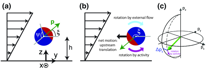
Figure 2: (a) Schematic description of the particle dynamics if the director $\mathbf{p}=(p_{x},p_{y},p_{z})$ (green) lies in the indicated shear plane. The angle $\xi$ is formed by the director and the flow direction. The wall is located at $z=0$ and $h$ is the distance of the particle center from the wall. For a catalytic Janus particle, the angle $\psi$ characterizes the size of the catalytic cap (blue). Note that here $\psi$ is larger than in Fig. 1. (b) Illustration of a particle in a rheotactic steady state which occurs for $p_{y}^{*}<0$ and $p_{z}^{*}<0$, i.e., for $\xi$ within the range $\pi<\xi<3\pi/2$. The external flow contributes a clockwise component $-\frac{1}{2}\dot{\gamma}f(h/R)\hat{x}$ (cyan) to the particle angular velocity (Eq. (II.2)). For the angle $\xi$ to remain stationary, the swimming activity of the particle must contribute a counterclockwise component (magenta) with equal magnitude to the angular velocity. Since the particle, assumed to be axisymmetric, does not rotate in free space, i.e., without the wall and in the absence of the external shear flow, this contribution must be due to the interaction with the wall. If the swimming velocity of the particle is large enough, the particle swims upstream. (c) Upstream rheotaxis is stable against perturbations of the director out of the shear plane, where $p_{x}=0$. Shear flow tends to rotate the director around the $\hat{x}$ direction, keeping $p_{x}$ constant and thus does not contribute to $\dot{p}_{x}$ (see the last paragraph in Subsec. II.C). The swimming activity of the particle tends to rotate the orientation vector along “lines of longitude” on the unit sphere $|\mathbf{p}|=1$. For a small perturbation $\Delta p_{x}$ (blue line segment) away from the rheotactic state shown in (b), activity rotates the director (green vector) towards the pole $p_{z}=-1$, decreasing $p_{x}$ and $p_{y}$ due to $|\mathbf{p}|=1$. The effect of activity is indicated by the magenta arrow.

II.4 Linear stability analysis of the fixed point $p_{x}^{*}=0$

In order to establish the conditions under which the fixed point $p_{x}^{*}=0$ (case (iii) above) is stable, so that the corresponding steady state exhibits rheotaxis, we proceed by carrying out a linear stability analysis. Since for $p_{x}=0$ the director lies within the shear plane and, due to the symmetry of the problem, cannot rotate out of this plane, in the three-dimensional phase space defined by $p_{x}$, $p_{z}$, and $h$ a trajectory with initial condition in the plane $p_{x}=0$ will be confined to that plane for all times $t$. Upon linearization of the equations of motion near the fixed point, a small perturbation $\Delta p_{x}$ decouples from the other variables:

$$\frac{d\Delta{p}_{x}}{dt}=-\frac{\Omega_{a,x^{\prime}}(p_{z}^{*},h^{*}/R)p_{z}^{*}}{\sqrt{1-p_{z}^{*2}}}\Delta{p}_{x}.$$ (8)

After using Eq. (II.3) for substituting
$\text{sgn}(p_{y}^{*})\,\Omega_{a,x^{\prime}}(p_{z}^{*},h^{*}/R)=\frac{1}{2}\dot{\gamma}f(h^{*}/R)$, we obtain

$$\frac{d\Delta{p}_{x}}{dt}=-\frac{\dot{\gamma}f(h^{*}/R)p_{z}^{*}}{2p_{y}^{*}}\Delta{p}_{x}\,.$$ (9)

Therefore $\Delta p_{x}$ decays or grows exponentially,

$$\Delta{p}_{x}=\Delta p_{x}(0)\exp\left(\frac{-\dot{\gamma}f(h^{*}/R)p_{z}^{*}}{2p_{y}^{*}}\,t\right)\,,$$ (10)

depending on the sign of the quantity multiplying $t$ in the argument of the exponential.

Since $f(h^{*}/R)>0$ and $\dot{\gamma}>0$, the stability of the fixed point is determined by the sign of the ratio $p_{z}^{*}/p_{y}^{*}$. For the particle to swim oriented upstream (i.e., to exhibit “positive” rheotaxis), it must align against the flow, so that $p_{y}^{*}<0$; stability then requires that $p_{z}^{*}<0$, i.e., the director points towards the wall. Additionally, if the swimming velocity is large enough to overcome the shear flow, i.e., for $\dot{y}_{p}<0$, where $\dot{y}_{p}=-U_{a,y^{\prime}}+\dot{\gamma}h^{*}g(h^{*}/R)$ (see $U_{f,y}$ in Eq. (II.2) and $U_{a,y}$ in Eq. (II.2) with $\phi=270^{\circ}$), net upstream swimming emerges. The other possibility, that an attractor exists for which $p_{y}^{*}$ and $p_{z}^{*}$ are both positive, is in general unlikely, because the particle would be pointing away from the wall (see Fig. 1(a)). Furthermore, it would correspond to the less interesting case of negative rheotaxis, in which the particle motion is in the flow direction. Therefore, it will not be discussed further.

The analysis of the linear stability shows that we need to examine particle dynamics only in the symmetry plane $p_{x}=0$ in order to determine whether rheotaxis occurs. In the following, we shall examine the two-dimensional dynamics in this plane in detail. Additionally, we shall perform fully three-dimensional numerical calculations of trajectories with initial conditions $p_{x}(t=0)\neq 0$ in order to explore the limits of validity of the linear analysis, as well as to understand the details of the evolution towards alignment in the shear plane. We introduce a new angle $\xi$, shown in Fig. 2(a), which will turn out to be convenient for describing the director orientation if $p_{x}=0$. The requirement that the attractor occurs with $p_{y}^{*}<0$ and $p_{z}^{*}<0$ translates into $\pi<\xi^{*}<3\pi/2$.

Before proceeding with the analysis, we discuss the physical picture behind the stability criteria in Eq. (10). While we have provided mathematical conditions for rheotaxis, the corresponding physical interpretation can provide further insight. Equation (3) shows that particle activity has an effect on $p_{x}$, but shear does not. The contribution of shear to the angular velocity of the particle is rigid rotation around the $\hat{x}$ axis. In the absence of activity, shear rotates the tip of the director in a coaxial circle around the $\hat{x}$ axis, keeping $p_{x}$ constant. Now we consider activity. Due to the mirror symmetry with respect to the plane containing $\mathbf{p}$, the contribution of activity can only drive rotation of the director with arbitrary orientation $\mathbf{p}$ towards or away from the planar wall. On the spherical surface defined by $|\mathbf{p}|=1$, this corresponds to rotation of the director along a line of longitude, where $p_{z}=1$ and $p_{z}=-1$ define the poles [Fig. 2(c)]. The question, then, is whether, for a small perturbation $\Delta p_{x}$, activity will tend to drive the director towards the equator $p_{z}=0$ of $|\mathbf{p}|=1$ or towards the nearest pole. From Fig. 2(c) we note that the effect of the small perturbation $\Delta p_{x}$ is to shift the tip of the director to a neighboring line of longitude. Therefore, if activity tends to rotate the director towards the equator, $\Delta p_{x}$ will increase (see Fig. 2(c)) because the distance between neighboring lines of longitude increases as they approach the equator from the pole. The direction of this activity induced rotation (i.e., towards the pole or towards the equator) is determined by the value of $\xi^{*}$. For instance, consider a positive rheotactic state, for which $\pi<\xi^{*}<3\pi/2$. In order to balance rotation by shear, activity must tend to rotate the director towards the pole $p_{z}=-1$, as shown in Fig. 2(b) and (c). Hence, this dynamical fixed point is stable against small perturbations in $p_{x}$.

II.5 Calculation of the slip velocity

Finally, we briefly outline the calculation (if necessary) of the slip velocity $\mathbf{v}_{s}=v_{s,\theta_{p}}\hat{\mathbf{e}}^{\prime}_{\theta_{p}}$ (where $\hat{\mathbf{e}}^{\prime}_{\theta_{p}}$ denotes the unit vector in the primed coordinate frame corresponding to the polar angle $\theta_{p}$ measured from the director, i.e., the symmetry axis of the particle) along the surface of the spherical particle which, for the specific swimmer models considered here, is an input to the problem outlined in Subsec. II.A.

For a “squirmer”, $\mathbf{v}_{s}$ is specified by fiat and does not depend on the configuration $(\mathbf{p},h)$ of the particle. Following Li and Ardekani Li and Ardekani (2014), we consider a squirmer for which the slip velocity is given by

$$v_{s,\theta_{p}}=B_{1}\sin(\theta_{p})+B_{2}\sin(\theta_{p})\cos(\theta_{p}),$$ (11)

The model is characterized by the squirming mode amplitudes $B_{1}$ and $B_{2}$. In an unconfined quiescent fluid (i.e., free space) such a squirmer moves with velocity $U_{f.s.}=(2/3)B_{1}$.

A self-phoretic Janus particle generates solute molecules over the surface of a catalytic cap. We parameterize the extent of the cap by $\chi_{0}=-\cos(\psi)$, where the angle $\psi$ is defined in Fig. 2(a). It is assumed that the interaction between the active particle and the (non-uniformly distributed) solute molecules has a range much smaller than $R$ and $h$. Thus it can be accounted for as driving a tangential flow in a thin boundary layer of thickness $\delta<<R,h$ surrounding the particle. This can be modeled as an effective slip velocity $\mathbf{v}_{s}=-b(\mathbf{r})\nabla_{||}c(\mathbf{r})$, where $c(\mathbf{r})$ is the solute number density field Anderson (1989); Golestanian et al. (2005). The operator $\nabla_{||}=(\mathbf{1}-\mathbf{n}\mathbf{n})\cdot\nabla$ is the projection of the gradient onto the active particle surface, with $\mathbf{n}$ denoting the surface normal oriented into the fluid. The quantity $b(\mathbf{r})$ is the so-called “surface mobility,” determined by the details of the interaction between the active particle and the solute molecules. For instance, the sign of $b$ expresses whether the active particle is attracted to or repelled from the solute molecules. Throughout the present study, we assume repulsion. Since the solute number density $c(\mathbf{r})$ is affected by the presence of the wall, in this model the slip velocity $\mathbf{v}_{s}$ depends on the configuration $(\mathbf{p},h)$.

If the effect of advection on $c(\mathbf{r})$ can be neglected, one can determine $c(\mathbf{r})$ (and with this $\mathbf{v}_{s}$) prior to the consideration of the hydrodynamic problem posed in Subsec. II.A (see, e.g., Refs. Anderson (1989); Popescu et al. (2009)). (Within this approach it is disregarded how the flow field $\mathbf{u}$ couples back to $c(\mathbf{r})$.) In this case, the solute number density is quasi-static, and obeys the Laplace equation $D\nabla^{2}c=0$, subject to the boundary conditions for the normal derivatives $\hat{n}\cdot\nabla c=0$ on the wall, $\hat{n}\cdot\nabla c=0$ over the inert surface of the colloid, and $-D(\hat{n}\cdot\nabla c)=\kappa$ on the catalytic cap. The quantity $D$ is the diffusion coefficient of the solute molecules, and $\kappa$ is the flux of solute per unit area from the catalytically active cap. Concerning the first and second boundary conditions, the wall and the inert surface of the particle are taken to be completely impenetrable to solute molecules. In the third boundary condition, it is assumed that the rate of the reaction is independent of the local concentration of solute molecules.

It is valid to neglect advective effects if the Péclet numbers $Pe\equiv U_{f.s.}R/D$ and $Pe_{\dot{\gamma}}\equiv\dot{\gamma}R^{2}/D$ are small, where $U_{f.s.}$ is the particle velocity in free space. (The Péclet number $Pe$ is the ratio between the time scale for solute to diffuse a distance $R$ and the timescale for the particle to move a distance $R$. Similarly, the Péclet number $Pe_{\dot{\gamma}}$ characterizes the advection of the solute molecules by the external flow, for which the velocity scale is $\dot{\gamma}R$, relative to the diffusion of the solute molecules Frankel and Khair (2014).) Additionally, we assume that the Reynolds number $Re\equiv\rho U_{f.s.}R/\mu$ (where $\rho$ is the mass density of the suspending fluid and $\mu$ is its dynamic viscosity) is small, permitting the use of the Stokes equations to account for the hydrodynamics. For example, a self-propelled Janus colloid which catalyzes the decomposition of hydrogen peroxide into water and oxygen typically has a diameter of $\sim 5\;\mathrm{\mu m}$ and moves with a velocity $\sim U_{f.s.}=5\;\mathrm{\mu m/s}$ through the aqueous solution ($\rho\simeq 10^{3}\;\mathrm{kg/m^{3}}$ and $\mu\simeq 10^{-3}\;\mathrm{Pa\,\times\,s}$). In this case, $Re\approx 10^{-5}$. Furthermore, estimating the diffusion coefficient of oxygen in water as $D\simeq 4\times 10^{-9}\;\mathrm{m^{2}/s}$, we obtain $Pe\approx 10^{-3}$ Popescu et al. (2010). A representative shear rate in microfluidic devices is $\dot{\gamma}=1\;\mathrm{s^{-1}}$ (see, for instance, Refs. Kantsler et al. (2014) and Chengala et al. (2013)), which renders $Pe_{\dot{\gamma}}\approx 10^{-3}$. Thus for typical active particles the above assumptions of small $Pe$, $Pe_{\dot{\gamma}}$, and $Re$ numbers are well justified.

Before proceeding to an analysis of the numerical results, we remark on the physical realizations which would be captured by our model. In many experiments, the catalytic reactions involve more than one product as well as possibly a number of reactants. If the system remains in a reaction-rate limited regime (i.e., the reactants are in abundance and transported sufficiently fast so that there is no noticeable depletion near the catalyst), accounting for more than one product means to modify the expression for the slip velocity in a linear manner: the gradient of each reaction product “i” multiplied by its corresponding surface mobility $b_{i}$ is simply added in order to obtain the phoretic slip around the particle. In this case, the results presented here can be easily extended by replacing the effective number density $c$ by the sum over the densities of all products with an effective $b$ such that $b\nabla_{||}c\rightarrow b_{1}\nabla_{||}c_{1}+b_{2}\nabla_{||}c_{2}+...$. On the other hand, if the catalytic reaction is diffusion limited and involves at least two reactants, the source boundary condition at the catalytic-active region involves products of the densities of the reactants. In this case the equations describing the system become nonlinear, and the present model is neither applicable, nor does it lend itself to an obvious extension.

III Numerical Results and Discussion

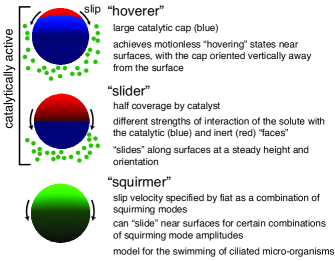
Figure 3: Illustration of the three types of spherical active particles studied here numerically. The three types differ in the kind of their surface activity. A catalytically active particle generates solute molecules (green discs) over the surface of a catalytic cap (blue). The interaction between the solute and the particle surface, here taken to be repulsive, drives a surface flow (slip velocity) as discussed in the main text, leading to a motion of the particle away from its cap. A “hoverer” (Sec. III.1) exhibits a very high coverage by catalyst. As discussed in Ref. Uspal et al. (2015), if it is near a planar wall it can achieve a motionless “hovering” state at a steady height above the wall and with the cap oriented away from the wall (as shown in Fig. 4, left panel). For the hoverer considered here, we take the solute to interact identically with the catalytic and inert “faces” of the particle. In contrast, the “slider” considered in Sec. III.2 is only half covered by catalyst, but the solute interacts more strongly with its catalytic face (blue) than with its inert face (red). This particle tends to swim along surfaces at a steady height and orientation, or “slides.” Finally, for the “squirmer”(Sec. III.3), the slip velocity is not due to a self-generated distribution of solute, but rather it is specified by fiat as a combination of “squirming modes.” For certain combinations of squirming mode amplitudes, the squirmer can achieve sliding state, too.

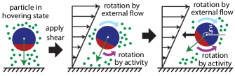
Figure 4: Schematic illustration of a dynamical process through which a “hoverer” particle can achieve a rheotactic state. Left panel: The particle is initially in a “hovering” state without any external flow. As discussed in Ref. Uspal et al. (2015), the catalytic cap of the particle (blue) generates solute molecules (green discs), which interact with the particle surface via a repulsive potential. A “cushion” of repulsive solute in the space between the particle and the hard planar wall exactly balances the tendency of the particle to swim away from its cap. Center panel: An external shear flow tends to rotate the particle clockwise (cyan arrow). The near-wall chemical activity of the particle tends to rotate the particle back to the hovering orientation (magneta arrow). However, this contribution to particle rotation is small for a small displacement from the hovering orientation. The net effect is that the particle rotates away from the hovering orientation. Right panel: For sufficiently large displacements of the angle $\xi$ from the hovering state value $\xi=3\pi/2$, the two contributions to particle rotation balance, and a steady angle is achieved. Simultaneously, the particle still achieves a steady height above the wall due to the solute “cushion” effect. As a result, the particle translates upstream (black arrow), as its catalytic cap (blue) is oriented slightly downstream.

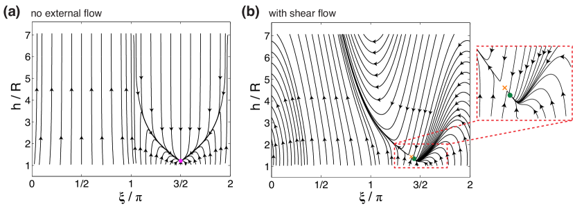
Figure 5: (a) Phase plane for a Janus particle with high coverage by catalyst ($\chi_{0}=0.85$) and uniform surface mobility if the director lies in the $yz$ plane ($p_{x}=0$) and if there is no external flow. The filled magenta circle indicates an attractive “hovering” state. In this state, the particle remains motionless at a height $h^{*}/R=1.21$, with its cap oriented vertically and away from the wall ($\xi^{*}=3\pi/20=270^{\circ}$). The tendency of the particle to move away from its cap is balanced by the accumulation of solute near the wall. Clearly, the basin of attraction for this state is large. Additionally, many trajectories (roughly speaking, the whole basin of attraction) converge without overlapping to a “slow manifold” (the two visible branches merging into the attractor), indicative of two timescale dynamics: the vertical motion is much faster than the rotation of the particle Uspal et al. (2015). Trajectories with an initial angle $0<\xi_{0}/\pi<1$ escape from the wall. The mirror symmetry of the region $1<\xi/\pi<2$ across $\xi/\pi=3/2$, as well as the mirror symmetry of the region $0<\xi/\pi<1$ across $\xi/\pi=1/2$, is due to rotational symmetry around the $\hat{z}$ axis in the absence of flow. (b) Phase plane for the same Janus particle if the director lies in the shear plane ($p_{x}=0$) and in the presence of a shear flow with $\dot{\gamma}R/U_{0}=0.02$. Note that the phase plane is periodic in the $\xi$ direction. Due to the rotation of the particle by the flow, the attractor (filled green circle) has migrated into the region $1<\xi/\pi<3/2$, and is now at $h^{*}/R=1.35$ and $\xi^{*}=257^{\circ}$. As discussed in Sec. II, this is the region in which positive rheotaxis is possible. A particle in this state moves upstream with a steady height and orientation. The orange cross indicates a saddle point. An enlarged view of the region containing the saddle point and the attractor is provided in the right panel; some trajectories have been omitted for clarity.

When considering a Janus particle, we use the boundary element method (BEM) in order to solve the diffusion equation for the solute number density field $c(\mathbf{r})$. Additionally, for both propulsion mechanisms (the squirmer and the catalytically active particle), we use the BEM in order to solve the hydrodynamic subproblems I and II. A detailed introduction to the BEM is provided by Pozrikidis Pozrikidis (2002). We adopted his freely available BEMLIB code and modified it for the present study. For subproblem I, we calculate $f(h/R)$ and $g(h/R)$ for an (inactive) sphere in a shear flow at various heights $h/R$. We find that the numerically obtained values are in good agreement with the analytically obtained values given by Goldman et al Goldman et al. (1967). In a previous study, we provided a detailed description of how to apply the BEM in order to solve the diffusion equation (for a catalytic Janus particle) and subproblem II Uspal et al. (2015). Within this approach we have obtained $U_{a,z^{\prime}}$ and $\Omega_{a,x^{\prime}}$ on a grid of $h$ and $\theta$.

In order to determine full particle trajectories for an initial condition $(h_{0},\mathbf{p}_{0})$, we interpolate $f(h/R)$, $g(h/R)$, $U_{a,z^{\prime}}$, and $\Omega_{a,x^{\prime}}$ and integrate Eqs. (3) - (6) numerically. In the following, we restrict our numerical calculations to the region $1.02\leq h/R\leq 7.1$. Above $h/R=7.1$, we consider the particle to have “escaped” the surface. Below $h/R=1.02$, various of our physical approximations (e.g., that the effects of the solute distribution around the particle can be accounted for by a phoretic slip calculated within a thin layer, including that part of the surface of the particle which is in close proximity of the wall) are expected to break down. For a catalytic Janus particle, $U_{0}\equiv|b|\kappa/D$ provides a characteristic velocity, and $T_{0}\equiv R/U_{0}$ a characteristic timescale. For instance, it was shown analytically that a catalytic Janus particle with uniform surface mobility and half coverage by catalyst has a velocity $U_{f.s.}/U_{0}=1/4$ in free space Popescu et al. (2010). When we take the catalytic cap and the inert region to have unequal surface mobilities, we use $U_{0}\equiv|b_{cap}|\kappa/D$. Similarly, for squirmers the amplitude $B_{1}$ of the first squirming mode provides a characteristic velocity scale, and the time $T_{s}\equiv R/B_{1}$ a characteristic timescale. The ratio between the squirming mode amplitudes defines a parameter $B_{2}/B_{1}$. In each of the cases which we shall study in this section, the corresponding velocity and time scales defined above and the particle radius $R$ will be employed to render the dynamical equations, Eqs. (3) - (6), dimensionless.

First, we shall apply the theoretical results derived in the previous section to show that the surface chemistry of a catalytically active Janus particle can be tailored such that it leads to the occurrence of positive (upstream) rheotaxis. We shall provide two rather distinct examples of such a design of the surface properties, each exploiting a particular pathway to produce the stabilizing wall-induced rotation component discussed in Subsec. II.4. These two examples are depicted schematically in Fig. 3. In order to illustrate the generality of our theoretical results, we shall show that rheotaxis can occur for certain spherical squirmers.

Our approach to design is guided by the idea outlined in Fig. 2(b). For positive rheotaxis, the particle director $\mathbf{p}$ must point upstream and towards the wall. The external flow contributes a clockwise component, shown by the cyan arrow, to the angular velocity $\mathbf{\Omega}$ of the particle. For the particle to maintain a steady orientation, the near-wall swimming activity of the particle must contribute a counterclockwise component $\mathbf{\Omega}_{a}=-\mathbf{\Omega}_{f}$, shown by the magenta arrow, to $\mathbf{\Omega}=\mathbf{\Omega}_{f}+\mathbf{\Omega}_{a}$. Since the axisymmetric particle does not rotate in free space, the counterclockwise component $\mathbf{\Omega}_{a}$ must be due to the effect of the wall on the fluid velocity field and the solute number density field. Additionally, the particle must be attracted to a steady height through its near-wall swimming activity. In other words, the tendency of the particle to swim away from its cap must be counteracted by the effect of the wall on the fluid velocity and solute density field. In the following two subsections, we shall introduce two particle surface chemistries which fulfill these criteria. By tailoring the surface chemistry, we can turn on or off, and rationally control, various physical mechanisms which contribute to the particle motion.

We note that the following three subsections (corresponding to the three particle designs shown in Fig. 3) have a repetitive structure of arguments and presentation, so that the reader can choose to read the first subsection, skip ahead to the Conclusions, and return to read Subsections B and C at leisure.

III.1 Catalytic Janus particles with high coverage and uniform surface mobility

Previously Uspal et al. (2015) we studied the dynamics of a model catalytically active Janus particle suspended in a quiescent fluid and near a wall. We found that, for a uniform surface mobility $b$, in the course of time a particle with a very high coverage by catalyst can be stably attracted to a “hovering” state in which it remains motionless at a height $h^{*}$ and angle $\xi^{*}=3\pi/2$ (see Fig. 2(b)), i.e., with its catalytic cap oriented vertically and away from the wall Uspal et al. (2015). In this state, depicted in the left panel of Fig. 4, the tendency of the particle to translate away from its cap (i.e., trying to avoid high solute concentrations) is balanced by the accumulation of a solute “cushion” near the impenetrable wall (which is due to the confinement of the solute between the particle and the wall). The stability of this hovering state against perturbations in the $\hat{z}$ direction can be understood easily: if the particle moves closer to the wall, solute accumulation is enhanced, and repulsion from the wall is stronger; if the particle moves away from the wall, repulsion from the wall is weakened, but the particle still translates away from its cap. Less obviously, hydrodynamic interactions with the wall stabilize the particle against perturbations in the angle $\xi$. Hydrodynamically, the particle is characterized as a “puller” (see the flow lines in Fig. 3(b) in Ref. Uspal et al. (2015)). Pullers are known to orient themselves perpendicular to planar surfaces via hydrodynamic interactions Spangolie and Lauga (2012).

The phase plane for a hoverer with $\chi_{0}\,\equiv-\cos\psi=0.85$ and uniform surface mobility $b$ in a quiescent fluid (i.e., no external flow) is shown in Fig. 5(a). The phase plane indicates the evolution of the particle configuration $(h,\xi)$ for any initial condition $(h_{0},\xi_{0})$. In the absence of flow, the system is symmetric for rotations around the $\hat{z}$ axis. This rotational symmetry is evinced by two mirror symmetries in the phase plane: symmetry of the region $0<\xi/\pi<1$ for reflection across $\xi/\pi=1/2$, and symmetry of the region $1<\xi/\pi<2$ for reflection across $\xi/\pi=3/2$. The “hovering” attractor is shown as a filled magenta circle at $\xi^{*}=3\pi/2$ and $h^{*}/R=1.21$. As discussed in Ref. Uspal et al. (2015), many trajectories in the basin of attraction are drawn to a “slow manifold” indicative of two timescale dynamics: rotation is much slower than motion in $\hat{z}$ direction. For initial conditions $\xi_{0}<\pi$, the particle escapes the surface.

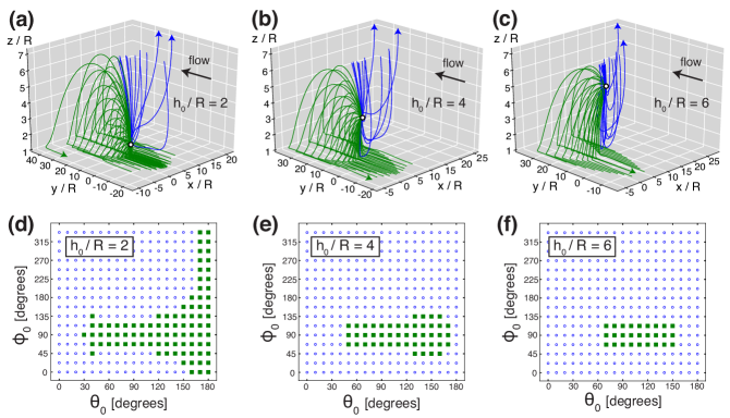
Figure 6: Trajectories and phase maps for a catalytic Janus particle with high coverage by catalyst ($\chi_{0}=0.85$) and uniform surface mobility. A trajectory starts from an initial height $h_{0}$, an initial director orientation $\theta_{0}$ and $\phi_{0}$, and an initial lateral position $(x_{0},y_{0})=(0,0)$. There is an ambient shear flow with dimensionless shear rate $\dot{\gamma}R/U_{0}=0.02$. The panels (a), (b), and (c) show trajectories launched from $h_{0}/R=2$, $h_{0}/R=4$, and $h_{0}/R=6$, respectively. Green trajectories are attracted to a rheotactic swimming state, whereas blue trajectories escape from the surface. In each panel, a white circle shows the initial spatial position of all trajectories. Arrowheads on selected trajectories indicate the direction of motion. In panels (d), (e), and (f) we show phase maps which indicate the behavior for each initial height and orientation. The filled green squares correspond to the rheotactic trajectories, and the open blue circles correspond to the escaping trajectories. Note that, for visual clarity, not all of the trajectories considered in (d) through (f) are plotted in (a) through (c). In particular, escaping trajectories are only shown in the region $x>0$.

Now we consider the same “hoverer” in shear flow. The flow will rotate the particle clockwise, decreasing $\xi$ from $\xi=3\pi/2$. On the other hand, the hydrodynamic interaction which stabilized “hovering” will tend to rotate the particle back towards $\xi=3\pi/2$. As depicted in the center and right panels of Fig. 4, these two contributions to rotation can balance for sufficiently large angular displacement from the cap-down orientation. Hence the right panel of Fig. 4 provides a potential realization of the mechanism illustrated in Fig. 2. Therefore we anticipate that, at least for sufficiently slow external flows, there will a stable angle $\pi<\xi^{*}<3\pi/2$. Moreover, we anticipate that the “cushion” effect will be preserved to produce a steady height $h^{*}$. The numerical simulations for, e.g., $\dot{\gamma}R/U_{0}=0.02$ lead to a phase plane as shown in Fig. 5(b) and confirm these expectations: the attractor (filled green circle) is preserved and it migrates into the region $1<\xi/\pi<3/2$, being now located at $h^{*}/R=1.35$ and $\xi^{*}=257^{\circ}$. Trajectories from a large section of phase space are drawn to this attractor. (Note that the phase plane is periodic in the $\xi$ direction.) Additionally, we indicate a saddle point (orange cross). The saddle point and attractor are rather close, as we have chosen a shear rate close to the (numerically estimated) upper critical value $\dot{\gamma}_{c}\approx 0.021\times U_{0}/R$. At the critical value, the saddle point and the attractor collide and annihilate each other. Above the critical shear rate, there is no stable rheotaxis, and, for this choice of the surface chemistry, all trajectories escape from the surface. We have chosen $\dot{\gamma}R/U_{0}$ near the upper critical shear rate since, as will be discussed in the Conclusions, “strong” external flows have the greatest experimental relevance and accessibility. Additionally, the relaxation time scale in Eq. (10) decreases as the shear rate is increased. Therefore, we expect the approach towards the rheotactic state to occur most rapidly for $\dot{\gamma}R/U_{0}$ being close to the upper critical shear rate. Although we leave an exhaustive parametric study to future research, we note that results of additional numerical calculations at lower values of $\dot{\gamma}R/U_{0}$, omitted here, agree with this expectation.

Since the attractor is in the region $\pi<\xi^{*}<3\pi/2$, it should be stable against perturbations of the director out of the shear plane, as discussed in Sec. II. In order to probe the stability of the attractor and its basin of attraction, we consider an ensemble of trajectories launched from various initial director angles $\theta_{0}$ and $\phi_{0}$ (see Fig. 1(a)), initial heights $h_{0}/R=2$, $h_{0}/R=4$, and $h_{0}/R=6$, and the initial lateral position $(x_{0},y_{0})=(0,0)$. For these three initial heights Figs. 6(a), (b), and (c) show three-dimensional trajectories of the coordinates $(x,y,z)$ of the centers of the particles. Each trajectory has been obtained from an initial position and orientation by numerically integrating Eqs. (3)-(6). Green trajectories are “rheotactic.” Particles following these trajectories are attracted to the steady height $h^{*}/R=1.35$ and angle $\xi^{*}=257^{\circ}$ and move upstream. Particles following blue trajectories escape from the surface (i.e., the trajectories cross $h/R=7.1$ from below.) Phase maps, indicating how the particle behavior depends on the initial height and orientation, are shown in Figs. 6(d), (e), and (f), which correspond to $h_{0}/R=2$, $h_{0}/R=4$, and $h_{0}/R=6$, respectively. Clearly, rheotaxis is achieved for a large basin of initial conditions.

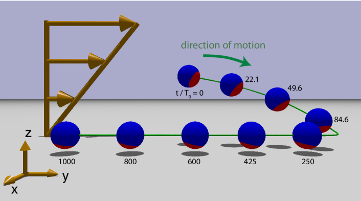
Figure 7: Trajectory for a catalytic Janus particle with high coverage by catalyst ($\chi_{0}=0.85$, blue) and uniform surface mobility for the initial conditions $h_{0}/R=6$, $\theta_{0}=120^{\circ}$, and $\phi_{0}=67.5^{\circ}$ in a shear flow with $\dot{\gamma}R/U_{0}=0.02$. The particle is attracted to a configuration in which it is tilted slightly away from the “hovering” state (i.e., a completely vertical orientation) by the flow, and consequently moves upstream. Particle positions along the trajectory are labeled by the dimensionless times $t/T_{0}$ at which they occur. The particle is clearly almost in the rheotactic state at $t/T_{0}=250$, which we estimate in the Conclusions to correspond to $t\sim 30\,\textrm{s}$ for typical catalytic Janus particles used in experiments. Note that we have slightly enlarged the appearance of the inert part of the particle surface for visual clarity. For this trajectory, the time dependence of various quantities is shown by solid lines with stars in Fig. 9.

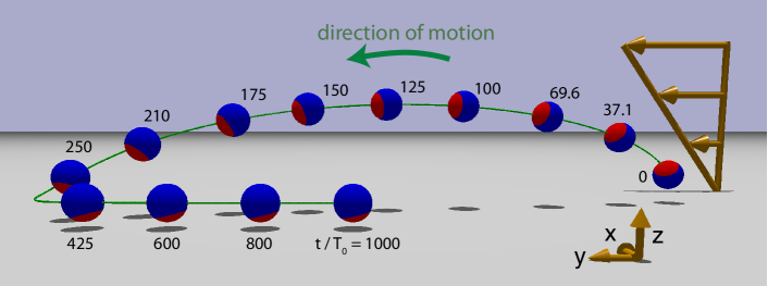
Figure 8: Trajectory for a catalytic Janus particle with high coverage by catalyst ($\chi_{0}=0.85$, blue) and uniform surface mobility for the initial conditions $h_{0}/R=2$, $\theta_{0}=40^{\circ}$, and $\phi_{0}=135^{\circ}$ in a shear flow with $\dot{\gamma}R/U_{0}=0.02$. The particle initially moves away from the wall, owing to the orientation of its catalytic cap. A few particle diameters away from the wall, the influence of the wall is very weak. However, the particle is rotated by the flow to move back towards the wall. As the particle approaches the wall, the influence of the wall strengthens. The particle rotates into the “tilted hoverer” configuration and moves upstream. Particle positions along the trajectory are labeled by the dimensionless times $t/T_{0}$ at which they occur. Note that we have slightly enlarged the appearance of the inert part of the particle surface for visual clarity. For this trajectory, the time dependence of various quantities is shown by solid lines with squares in Fig. 9.

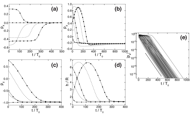
Figure 9: (a)-(d) Time evolution of various quantities for five of the rheotactic trajectories of the catalytic Janus particle considered in Fig. 6. The quantity $p_{x}$ decays to zero, while $p_{y}$, $p_{z}$, and $h$ attain asymptotically non-zero values $p_{y}^{*}=-0.22$, $p_{z}^{*}=-0.98$, and $h^{*}/R=1.35$. The initial conditions for these trajectories are: solid line with stars, $h_{0}/R=6$, $\theta_{0}=120^{\circ}$, $\phi_{0}=67.5^{\circ}$ (see also Fig. 7); solid line with filled circles, $h_{0}/R=2$, $\theta_{0}=180^{\circ}$, $\phi_{0}=0^{\circ}$; dotted line, $h_{0}/R=4$, $\theta_{0}=130^{\circ}$, $\phi_{0}=135^{\circ}$; dashed line, $h_{0}/R=6$, $\theta_{0}=70^{\circ}$, $\phi_{0}=112.5^{\circ}$; solid line with squares, $h_{0}/R=2$, $\theta_{0}=40^{\circ}$, $\phi_{0}=135^{\circ}$ (see also Fig. 8). In panel (e), $|p_{x}|$ is plotted for all studied rheotactic trajectories on a semi-logarithmic scale. The exponential character of the decay of $\left|p_{x}\right|$ is clearly visible. The slope of the dotted black line indicates the exponential time dependence predicted by Eq. (10).

An example of a rheotactic trajectory is shown in Fig. 7. Starting from the initial orientation $h_{0}/R=6$, $\theta_{0}=120^{\circ}$, and $\phi_{0}=67.5^{\circ}$, the particle has nearly attained the steady height and orientation after moving only a few particle diameters. The particle is attracted to a configuration in which it is tilted slightly away from the “hovering” state by the shear flow. As the (blue) cap is oriented slightly downstream (i.e., $\xi^{*}=257^{\circ}<270^{\circ}$), the particle moves upstream. In Fig. 8, the particle starts near the wall, but pointing away from it. Due to this initial orientation, the particle moves a few diameters away from the wall, where the hydrodynamic and chemical influence of the wall is very weak. However, the flow rotates the particle to swim back towards the wall. Upon returning to the vicinity of the wall, the particle rotates into the “tilted hoverer” configuration.

For selected rheotactic trajectories, in Fig. 9 we plot the time evolution of the particle height and of the components of the director. As expected, the component $p_{x}$ of the director perpendicular to the shear plane decays to zero. The height $h$ and the two in-plane components $p_{y}$ and $p_{z}$ attain asymptotically non-zero values. In Fig. 9(e), we plot the time evolution of $\left|p_{x}\right|$ for all rheotactic trajectories studied for Fig. 6. The decay of $\left|p_{x}\right|$ is clearly exponential, and the timescale for decay closely agrees with the prediction of Eq. (10), which is plotted as the dotted line in Fig. 9(e). Note that in Figs. 7, 8, and 9 time is given in dimensionless units as $t/T_{0}$. In a previous section, $T_{0}$ has been defined as $T_{0}\equiv U_{0}/R$. As will be discussed in the Conclusions, we estimate $T_{0}$ to be $T_{0}\approx 0.125\,\textrm{s}$ for catalytic Janus particles as typically used in experiments.

III.2 Catalytic Janus particle: half coverage and inhomogeneous surface mobilities

In order to demonstrate the general character of our theoretical findings, we seek to reach the rheotactic state of Fig. 2(b) via the alternative pathway of a different surface chemistry designed to realize a distinct physical mechanism. Specifically, we consider a particle which is half covered by catalyst ($\chi_{0}=0$), but the surface mobilities of the inert region and of the catalytic cap are taken to differ: $b_{inert}\neq b_{cap}$. In part, this choice is motivated by the fact that by default experimental studies use particles with half coverage, because these can readily be prepared by vapor deposition. Moreover, since the catalytic and inert surface regions consist of different materials, they are likely to give rise to different surface mobilities, too.

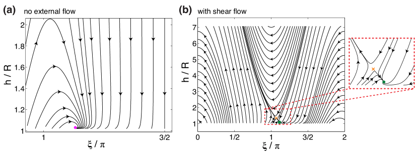
Figure 10: (a) Close-up of the phase plane of a Janus particle with half coverage ($\chi_{0}=0$) and inhomogeneous surface mobilities $b_{inert}/b_{cap}=0.3$ if the director is oriented in the $yz$ plane and there is no external flow. There is an attractor (filled magenta circle) at $h^{*}/R=1.03$ and $\xi^{*}=204^{\circ}$. At this point, the hydrodynamic interaction with the wall, which tends to rotate the cap towards the wall, is balanced by the effect of wall-induced chemical gradients, which tend to rotate the cap away from the wall. Importantly for the behavior in the presence of flow (see (b)), there is a region in which the net effect of the activity of the particle is to rotate the cap away from the wall. Within the region $1<\xi/\pi<3/2$, this occurs where the phase space trajectories in (a) flow towards larger $\xi$ (i.e., to the right.) (b) Phase plane for dynamics in the shear plane ($p_{x}=0$) of the same particle with an external shear flow $\dot{\gamma}R/U_{0}=0.05$. There is a rheotactic attractor (filled green circle) at $h^{*}/R=1.08$ and $\xi^{*}=200^{\circ}$, as well as a saddle point (orange cross). At the attractor, the net orientational effect of the chemical activity, which tends to rotate the cap away from the wall, is balanced by the orientational effect of the shear, which tends to rotate the cap towards the wall, as illustrated in Fig. 2(b). Note that the phase plane is periodic in $\xi$. An enlarged view of the region containing the saddle point and the attractor is provided in the right panel.

In our previous study of systems without flow, we have isolated two distinct wall-induced contributions to the rotation of a Janus particle Uspal et al. (2015). One contribution is due to the hydrodynamic interaction of the particle with the wall. Disturbance flows created by the motion of the particle are reflected by the wall, coupling back to the particle. We found that, for half coverage ($\chi_{0}=0$), hydrodynamic interactions always tend to rotate the catalytic cap of the particle towards the wall (and thus the director away from the wall). Therefore, this contribution to particle rotation cannot oppose the rotation by the shear flow (cyan arrow in Fig. 2(b)) for $\pi<\xi<3\pi/2$, i.e., it cannot provide the magenta arrow in Fig. 2(b). However, we also found that if $b_{inert}\neq b_{cap}$, wall-induced chemical gradients can contribute to particle rotation. If $b_{inert}/b_{cap}<1$, repulsion of the solute (i.e., the reaction product) from the inert region is weaker than repulsion from the catalytic cap. Accordingly, wall-induced chemical gradients (i.e., a higher concentration of solutes on the side of the particle surface closer to the wall) tend to rotate the catalytically active cap away from the wall. (Note that chemical gradients will not drive rotation of the particle in the absence of the wall because the Janus particle is axially symmetric.) Therefore, taking $b_{inert}/b_{cap}<1$ generates a contribution to the rotational velocity of the particle which corresponds to the magenta arrow in Fig. 2(b).

Therefore, we consider a particle with half coverage ($\chi_{0}=0$) and $b_{inert}/b_{cap}=0.3$. A close-up of the phase plane for the dynamics is shown in Fig. 10(a) for the case that the director lies in the $yz$ plane and that there is no external flow. There is an attractor very close to the wall at $h^{*}/R=1.03$ and $\xi^{*}=204^{\circ}$. At this point, the hydrodynamic interaction with the wall, which tends to rotate the cap of the particle towards the wall, is balanced by the effect generated by wall-induced chemical gradients, which tends to rotate the cap away from the wall. The particle moves along the wall with a steady height and steady orientation, which we called a “sliding” steady state Uspal et al. (2015). Importantly, there are regions of the phase space in which the rotational effect of wall-induced chemical gradients is stronger than the rotational effect of the hydrodynamic interaction, such that in sum the cap tends to rotate away from the wall. In particular, in the interval $1<\xi/\pi<3/2$ in Fig. 10(a), the cap rotates away from the wall whenever trajectories flow towards larger $\xi$ (see Fig. 2(b)), i.e., to the right of the plot in Fig. 10(a). In this region, rotation away from the wall by chemical activity is so strong that it can balance the rotational effect of shear towards the wall, as illustrated in Fig. 2(b). In addition, $\dot{h}=0$ whenever the tangent to the trajectories $h(\xi)$ in Fig. 10(a) is horizontal, i.e., $d[h(\xi(t))]/dt=\dot{\xi}\,(dh/d\xi)=0$. Therefore, the swimming activity of the particle can potentially also on its own produce a steady height $h^{*}$. We also note that some trajectories cross below the minimum height $h/R=1.02$ which we consider. The particles seemingly “crash” into the wall. It is likely that many of these trajectories recross the line $h/R=1.02$ and flow to the attractor if the numerical calculations were extended below $h/R=1.02$; however, as discussed above, the physical approximations inherent in the calculations break down very close to the wall.

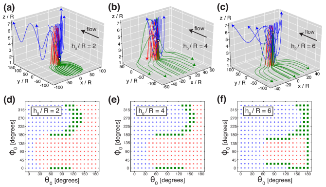
Figure 11: Trajectories and phase maps for a catalytic Janus particle with half coverage ($\chi_{0}=0$) and inhomogeneous surface mobilities $b_{inert}/b_{cap}=0.3$. A trajectory starts from an initial height $h_{0}$, an initial director orientation $\theta_{0}$ and $\phi_{0}$, and the initial lateral position $(x_{0},y_{0})=(0,0)$. There is an external shear flow with dimensionless shear rate $\dot{\gamma}R/U_{0}=0.05$. The panels (a), (b), and (c) show trajectories launched from $h_{0}/R=2$, $h_{0}/R=4$, and $h_{0}/R=6$, respectively. Green trajectories are attracted to a rheotactic swimming state, blue trajectories escape from the surface, and red trajectories “crash” into the wall (i.e., they approach the surface closer than the minimal height we consider numerically). In each panel, a white circle shows the initial spatial position of all trajectories. Arrowheads on selected trajectories indicate the direction of motion. In panels (d), (e), and (f) we show phase maps which indicate the behavior for each initial height and orientation. The filled green squares correspond to the rheotactic trajectories; the open blue circles correspond to the escaping trajectories; and the red crosses correspond to the “crashing” trajectories. Note that, for visual clarity, not all of the trajectories considered in (d) through (f) are plotted in (a) through (c).

We now consider the same particle in shear flow. The phase plane with shear rate $\dot{\gamma}R/U_{0}=0.05$ is shown in Fig. 10(b). As anticipated, there is a rheotactic attractor (filled green circle), which is located at $h^{*}/R=1.08$ and $\xi^{*}=200^{\circ}$. Additionally, there is a saddle point (orange cross). As in the case of the “hoverer,” we have chosen a shear rate close to the upper critical value (numerically estimated to be $\dot{\gamma}_{c}R/U_{0}\approx 0.06$ for this surface chemistry), and therefore the saddle point and attractor are very close to each other.

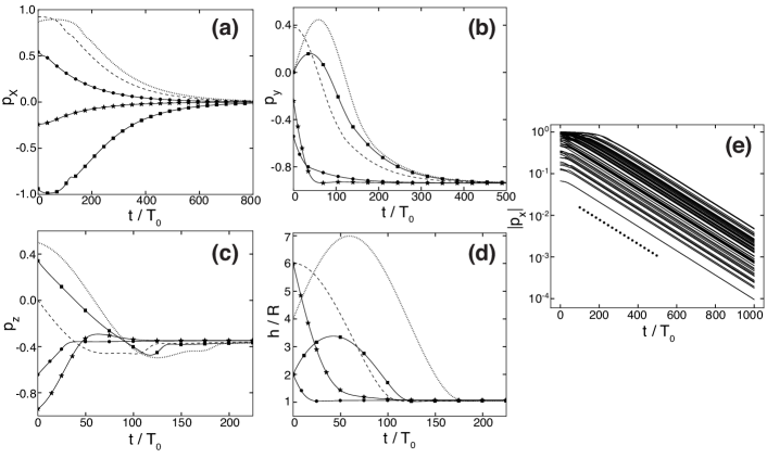
Figure 12: (a)-(d) Time evolution of $p_{x}$, $p_{y}$, $p_{z}$, and $h/R$ for five of the rheotactic trajectories considered in Fig. 11. The quantity $p_{x}$ decays to zero, while $p_{y}$, $p_{z}$, and $h$ attain asymptotically non-zero values $p_{y}^{*}=-0.94$, $p_{z}^{*}=-0.35$, and $h^{*}/R=1.08$. The initial conditions for these trajectories are: solid line with stars, $h_{0}/R=6$, $\theta_{0}=160^{\circ}$, $\phi_{0}=225^{\circ}$; solid line with filled circles, $h_{0}/R=2$, $\theta_{0}=130^{\circ}$, $\phi_{0}=315^{\circ}$; dotted line, $h_{0}/R=4$, $\theta_{0}=60^{\circ}$, $\phi_{0}=0^{\circ}$; dashed line, $h_{0}/R=6$, $\theta_{0}=90^{\circ}$, $\phi_{0}=22.5^{\circ}$ (see also Fig. 13); solid line with squares, $h_{0}/R=2$, $\theta_{0}=70^{\circ}$, $\phi_{0}=180^{\circ}$. In panel (e), $|p_{x}|$ is plotted for all studied rheotactic trajectories on a semi-logarithmic scale. The asymptotic decay of $\left|p_{x}\right|$ is clearly exponential. The slope of the dotted line indicates the exponential time dependence predicted by Eq. (10).

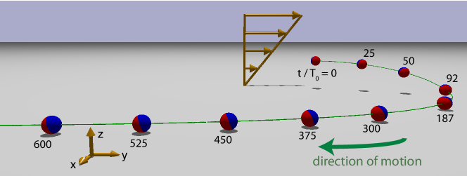
Figure 13: Trajectory for a catalytic Janus particle with half coverage ($\chi_{0}=0$) and inhomogeneous surface mobilities $b_{inert}/b_{cap}=0.3$ for the initial conditions $h_{0}/R=6$, $\theta_{0}=90^{\circ}$, and $\phi_{0}=22.5^{\circ}$ in a shear flow with $\dot{\gamma}R/U_{0}=0.05$. Particle positions along the trajectory are labeled by the dimensionless times $t/T_{0}$ at which they occur. The particle has “turned around” at $t/T_{0}=350$, which we estimate in the Conclusions to correspond to $t\sim 45\,\textrm{s}$ for typical catalytic Janus particles used in experiments. For this trajectory, the time dependence of various quantities is shown by dashed lines in Fig. 12.

As for Fig. 6, we launch an ensemble of particles from the lateral position $(x_{0},y_{0})=(0,0)$ of the center of the particles, for various initial director orientations $\theta_{0}$ and $\phi_{0}$, and heights $h_{0}/R=2$, $h_{0}/R=4$, and $h_{0}/R=6$. The three-dimensional trajectories of the center of the particles are shown in Figs. 11(a), (b), and (c). The green trajectories are rheotactic. Particles following blue trajectories escape from the surface. Finally, the red trajectories are those which “crash” into the surface, as discussed above. Phase maps indicating the particle behavior as a function of the initial orientation are shown in Figs. 11(d), (e), and (f). For selected rheotactic trajectories, in Fig. 12(a)-(d) we plot the time evolution of the height $h$ and of the director components $p_{x}$, $p_{y}$, and $p_{z}$. In Fig. 12(e), we plot $\left|p_{x}\right|$ for all rheotactic trajectories studied in Fig. 11. As in Fig. 9(e), the decay time for $p_{x}$ closely agrees with the prediction of Eq. (10), plotted as the dotted line in Fig. 12(e). Finally, a representative rheotactic trajectory is shown in detail in Fig. 13. The radius of curvature of the trajectory in its evolution towards the rheotactic steady state is clearly much larger than for the “hoverer” shown in Fig. 7. As with the hoverer, the dimensionless times $t/T_{0}$ in Figs. 12 and 13 can be converted to dimensional, and thus experimentally relevant values via the estimate $T_{0}\approx 0.125\,\textrm{s}$.

III.3 Squirmer

In order to further reveal the general character of our theoretical results and predictions, we consider a spherical “squirmer.” A squirmer has a prescribed surface velocity. It interacts with a bounding wall hydrodynamically, but not chemically, because the surface flow is not driven by a distribution of solute. The prescribed surface velocity is often taken to model the time-averaged motion of cilia on the surface of a micro-organism.

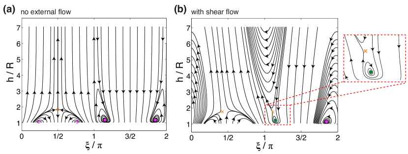
Figure 14: (a) Phase plane for a squirmer with $B_{2}/B_{1}=7$ (Eq. (11)) if the particle director lies in the $yz$ plane and if there is no external flow. There are stable dynamical attractors (filled magenta circles) for which the particle achieves a steady height and a steady orientation and “slides” along the wall. For these attractors, the particle director points towards the wall. There are also unstable fixed points (open magenta circles) and one saddle point (orange cross). Due to rotational symmetry around the $\hat{z}$ direction and in the absence of flow, the region $0<\xi/\pi<1$ is mirror symmetric across the line $\xi/\pi=1/2$, and the region $1<\xi/\pi<2$ is mirror symmetric across the line $\xi/\pi=3/2$. (b) Phase plane for the same squirmer if the particle director lies in the $yz$ plane and if there is a shear flow of strength $\dot{\gamma}R/B_{1}=0.09$. There is a rheotactic attractor (filled green circle). Since it lies in the region $1<\xi/\pi<3/2$, this attractor is stable against small perturbations of the director out of the $yz$ plane (i.e., for $p_{x}\neq 0$), as predicted in Sec. II. There is another fixed point (filled magenta circle) which is stable against perturbations within the plane $p_{x}=0$, but unstable against perturbations out of this plane. Likewise, this instability has been predicted in Sec. II for fixed points in the region $3/2<\xi/\pi<2$. There are two saddle points (orange crosses). The phase plane is periodic in the $\xi$ direction. An enlarged view of the region containing the rheotactic attractor and the nearby saddle point is provided in the right panel.

We follow Li and Ardekani Li and Ardekani (2014) in restricting our consideration to the first two squirming modes, given by $B_{1}$ and $B_{2}$ in Eq. (11). Li and Ardekani found that stable dynamical attractors exist for various values of $B_{2}/B_{1}$ and of the Reynolds number $Re$ Li and Ardekani (2014). (The lowest value of $Re$ they considered was $Re=0.1$.) For instance, for $B_{2}/B_{1}=3$ and $Re=1$, they found an attractor with $h^{*}/R=1.47$ and $\theta^{*}=103.2^{\circ}$. By construction our numerical method probes the limit $Re=0$. For $B_{2}/B_{1}=3$ (and $Re=0$), we have found an attractor at $h^{*}/R=1.64$ and $\theta^{*}=102.8^{\circ}$. We note that the dynamics of a squirmer near a boundary, including the possibility of moving at a stable height and orientation, was studied also by Ishimoto and Gaffney for $Re=0$ Ishimoto and Gaffney (2013).

Here, we consider a squirmer with $B_{2}/B_{1}=7$. We choose this large ratio in order to achieve a strong hydrodynamic interaction with the wall, permitting rheotaxis for a relatively high shear rate $\dot{\gamma}R/B_{1}=0.09$, as will be discussed below. (By comparison, for $B_{2}/B_{1}=3$ rheotactic states occur only for $\dot{\gamma}R/B_{1}<0.002$.) In Fig. 14(a) we show the phase plane for $B_{2}/B_{1}=7$ if the director lies in the $yz$ plane and if there is no external flow. There are two stable dynamical attractors (filled magenta circles) for which the particle moves at a steady height and a steady orientation with its director pointing towards the wall, similar to the “sliding” states we found for catalytic Janus particles Uspal et al. (2015). Due to the rotational symmetry of subproblem II (see Fig. 5 and the corresponding discussion in Sec. III.A), these two attractors are actually the same in the sense that they correspond to the same sliding state, only that the particle slides towards the negative and positive $\hat{y}$ direction for the attractor with $\xi^{*}/\pi<3/2$ and $\xi^{*}/\pi>3/2$, respectively. In addition, there are two unstable fixed points with $\xi^{*}/\pi<1$ (open magenta circles; this is again the same fixed point by symmetry) and a saddle point (orange cross).

Now we consider the effect of an external flow with $\dot{\gamma}R/B_{1}=0.09$ on the two attractors. They remain attractors for in-plane dynamics and stay at approximately the same locations in the phase plane, as can be seen in Fig. 14(b). The fixed point at $h^{*}/R=1.22$ and $\xi^{*}=207^{\circ}$ (filled green circle) lies in the region $1/2<\xi/\pi<3/2$ and therefore within the interval of $\xi$ for stable rheotaxis. In this configuration, the director is oriented upstream and towards the wall, as in Fig. 2(b). This fixed point is therefore a global attractor or an attractor for fully three-dimensional dynamics. For the other fixed point at $h^{*}/R=1.14$ and $\xi=332^{\circ}$ (filled magenta circle), the particle director is oriented downstream ($p_{y}>0$) and towards the wall ($p_{z}<0$); according to Eq. (10), this fixed point should be linearly unstable against perturbations out of the plane, i.e., away from $p_{x}=0$. In addition, there are two saddle points (orange crosses).

Figure 15: Trajectories and phase maps for a squirmer with $B_{2}/B_{1}=7$ (Eq. (11)). A trajectory starts from an initial height $h_{0}$, an initial director orientation $\theta_{0}$ and $\phi_{0}$, and the initial lateral position $(x_{0},y_{0})=(0,0)$. There is an external shear flow with dimensionless shear rate $\dot{\gamma}R/B_{1}=0.09$. The panels (a), (b), and (c) show trajectories launched from $h_{0}/R=2$, $h_{0}/R=4$, and $h_{0}/R=6$, respectively. Green trajectories are attracted to a rheotactic swimming state; blue trajectories escape from the surface; and red trajectories “crash” into the wall (i.e., they approach the surface closer than the minimal height we consider numerically). In each panel, a white circle shows the initial spatial position of all trajectories. Arrowheads on selected trajectories indicate the direction of motion. In panels (d), (e), and (f) we show phase maps which indicate the behavior for each initial height and orientation. The filled green squares correspond to rheotactic trajectories; the open blue circles correspond to the escaping trajectories; and the red crosses correspond to the “crashing” trajectories. Note that, for visual clarity, not all of the trajectories considered in (d) through (f) are plotted in (a) through (c).

As for Figs. 6 and 11, we launch an ensemble of particles from the lateral position $(x_{0},y_{0})=(0,0)$ of the center of the particles, for various initial angles $\theta_{0}$ and $\phi_{0}$, and heights $h_{0}/R=2$, $h_{0}/R=4$, and $h_{0}/R=6$. The three-dimensional trajectories of these particles are shown in Figs. 15(a), (b), and (c). Green indicates rheotactic trajectories; blue indicates trajectories which escape from the surface; and red trajectories “crash” into the wall (i.e., they approach the wall closer than $h/R=1.02$, which is the minimum height we consider numerically). The phase maps in Figs. 15(d), (e), and (f) indicate the particle behavior as a function of the initial height and the initial orientation. One rheotactic trajectory is shown in detail in Fig. 16.

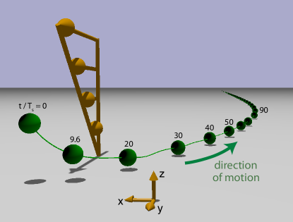
Figure 16: Rheotactic trajectory for a squirmer with $B_{2}/B_{1}=7$ and initial condition $h_{0}/R=6$, $\theta_{0}=130^{\circ}$, and $\phi_{0}=225^{\circ}$ in a shear flow with $\dot{\gamma}R/B_{1}=0.09$. The black shaded part of the particle indicates its rear. The trajectory exhibits oscillations. Selected particle positions along the trajectory are labeled by the dimensionless times $t/T_{s}$ at which they occur. For this trajectory, the time dependence of various quantities is shown by solid lines with stars in Fig. 17.

For selected rheotactic trajectories, in Figs. 17(a)-(d) we plot the time evolution of the height and of the orientation of the particle. Since the rheotactic attractor is oscillatory (see Fig. 14(b)), these quantities exhibit damped oscillations. The time evolution of $\left|p_{x}\right|$ for all rheotactic trajectories studied is plotted in Fig. 17(e). As for the catalytically active particles, the exponential decay of the component $p_{x}$ closely agrees with the one predicted by Eq. (10); in Fig. 17(e) this theoretical prediction is indicated by the slope of the dotted black line.

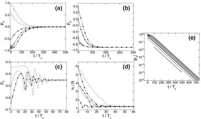
Figure 17: (a)-(d) Time evolution (in units of $T_{s}=R/B_{1}$) of various quantities for selected rheotactic trajectories of the squirmer discussed in Fig. 15. The quantity $p_{x}$ decays to zero, while $p_{y}$, $p_{z}$, and $h$ attain asymptotically non-zero values $p_{y}^{*}=-0.89$, $p_{z}^{*}=-0.45$, and $h^{*}/R=1.22$. The initial conditions for the trajectories are: solid line with stars, $h_{0}/R=6$, $\theta_{0}=130^{\circ}$, $\phi_{0}=225^{\circ}$ (see also Fig. 16); solid line with filled circles, $h_{0}/R=4$, $\theta_{0}=110^{\circ}$, $\phi_{0}=180^{\circ}$; dotted line, $h_{0}/R=4$, $\theta_{0}=120^{\circ}$, $\phi_{0}=315^{\circ}$; dashed line, $h_{0}/R=6$, $\theta_{0}=110^{\circ}$, $\phi_{0}=0^{\circ}$; solid line with squares, $h_{0}/R=2$, $\theta_{0}=110^{\circ}$, $\phi_{0}=157.5^{\circ}$. Note that, for visual clarity, in (c) only three trajectories are plotted. In (e), $\left|p_{x}\right|$ is plotted on a semi-logarithmic scale for all rheotactic trajectories studied. The slope of the dotted line indicates the exponential time dependence predicted by Eq. (10).

For the squirmer, we can test another prediction of the linear stability analysis. As discussed previously in Fig. 14(b), there is a fixed point, represented by the filled magenta circle, which is, as obtained numerically, a stable attractor for in-plane dynamics, i.e., for $p_{x}\equiv 0$. At this fixed point, the particle moves downstream at a steady height and a steady orientation. However, this fixed point lies in a region ($3/2<\xi/\pi<2$) for which linear stability analysis predicts fixed points to be unstable against small perturbations in $p_{x}$. In this context we launch two trajectories with initial conditions near this fixed point (Fig. 18). Both trajectories start with $h_{0}/R=1.2$ and $\theta_{0}=150^{\circ}$, but one with $\phi_{0}=90^{\circ}$ (dashed magenta line in Fig. 18(a)), i.e., $p_{x}=0$, and the other with $\phi_{0}=89^{\circ}$ (solid green line), i.e., $p_{x}\neq 0$. For the trajectory with $\phi_{0}=90^{\circ}$, the particle always remains in the shear plane ($p_{x}=0$) and is attracted to the downstream-moving state. However, for the trajectory with $\phi_{0}=89^{\circ}$, the particle moves out of the shear plane, and is ultimately attracted to the rheotactic upstream-moving configuration. In Fig. 18(b), we show the time evolution of $\left|p_{x}\right|$ for the rheotactic trajectory. Both the initial instability and the asymptotic approach to the rheotactic state clearly behave exponentially. The time dependences predicted by Eq. (10) are illustrated by dotted black lines. We note that the time scales for initial growth and asymptotic decay of $|p_{x}|$ are similar. This can be inferred from Fig. 14(b), in which the filled magenta circle and the filled green circle represent the downstream-moving and rheotactic upstream-moving fixed points, respectively. The original mirror symmetry across $\xi/\pi=3/2$ of Fig. 14(a), in which there is no external flow, is approximately preserved, and hence the two fixed points have approximately the same values of $|p_{y}^{*}|$, $|p_{z}^{*}|$, and $h^{*}$. (As a reminder, Fig. 2(a) relates $\mathbf{p}$ and $\xi$.) Since the time scale for growth or decay of $\Delta p_{x}$ is determined by $|p_{y}^{*}|$, $|p_{z}^{*}|$, and the local flow rate $\dot{\gamma}f(h^{*}/R)$ (see Eq. 10), the two time scales are approximately the same for the two fixed points.

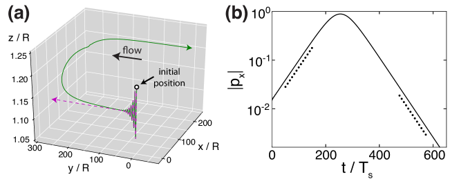
Figure 18: (a) Two trajectories with initial height and initial orientation near the fixed point represented by the filled magenta circle in Fig. 14(b). This fixed point is a stable attractor for in-plane dynamics, i.e., for $p_{x}\equiv 0$, but it is unstable against small perturbations in $p_{x}$. In this configuration, the particle moves in the downstream direction with a steady height and orientation. The two trajectories both have as initial conditions $h_{0}/R=1.2$ and $\theta_{0}=150^{\circ}$, as well as the same initial lateral position $(x_{0},y_{0})=(0,0)$ (white circle). However, one trajectory (magenta dashed line) has $\phi_{0}=90^{\circ}$, i.e., initially $p_{x}=0$, and therefore it is attracted to the downstream-moving state (i.e., the filled magenta circle in Fig. 14(b)). The other trajectory (solid green line) starts with $\phi_{0}=89^{\circ}$, i.e., initially $p_{x}\neq 0$, and ultimately it is attracted to the rheotactic upstream-moving state (i.e., the filled green circle in Fig. 14(b)). (b) The time evolution of $|p_{x}|$ in units of $T_{s}=R/B_{1}$ for the rheotactic ( green) trajectory of (a), plotted on a semi-logarithmic scale. The slopes of the dotted lines indicate the exponential time dependences predicted by Eq. (10).

IV Conclusions

We have theoretically investigated the possibility that a spherical active particle with propulsion mechanism, which (i) is axisymmetric and (ii) can be described in terms of an effective slip velocity, may exhibit rheotaxis (and, in particular, upstream rheotaxis) in shear flow near a planar surface. (We define rheotaxis as to denote the approach of the particle to a robust and stable steady state in which the orientation vector lies within the plane of shear). We have found that rheotaxis of such a particle is indeed possible, even though its spherical geometry rules out the intuitive “weather vane” mechanism generally invoked in order to explain rheotaxis for elongated microswimmers (e.g., sperm, E. coli, and polymer/hematite dimers.)

Furthermore, we have shown that for any such particles it is sufficient to analyze the dynamics of the particle with the orientation vector lying in the shear plane in order to determine whether or not rheotaxis occurs. In particular, for positive (upstream) rheotaxis, there must be an attractive steady state for the in-plane dynamics in which the orientation vector points upstream and towards the surface. For such a configuration, any small perturbation of the orientation vector out of the shear plane is damped by the moving activity of the particle. These findings significantly simplify the theoretical calculations. Moreover, they provide conceptually simple rules for the design of artificial rheotactic microswimmers. In order to achieve rheotaxis, one only needs to tailor the self-propulsion mechanism of the particle such that two criteria are satisfied: (i) the contribution of near-surface motion to the rotation of the particle can stably balance shear-induced rotation, as shown in Fig. 2(b), and (ii) the particle, through its near-surface moving activity, can achieve a steady state of fixed height. Specific examples of design for rheotaxis have been provided by exploring two distinct pathways for fulfilling these criteria via tailoring the surface chemistry of a catalytically active Janus particle. In the first pathway, the phoretic mobility is distributed homogeneously over the surface of the active particle, and the coverage by catalyst is adjusted to provide the required activity-induced rotation. In the second pathway, the coverage by catalyst is kept to the value of one half, which is simpler for experimental realizations, but the phoretic mobility is taken to be distributed inhomogeneously over the surface of the active particle. In both these cases, the numerical solutions of the equations of motion evidence rheotaxis and confirm the analytical prediction for the decay time for the component of the orientation vector out of the shear plane.

The numerical study we presented in Sec. III.A and B revealed the existence of a threshold value $r_{c}$ of the dimensionless parameter $r=\dot{\gamma}R/U_{0}$ above which rheotaxis is no longer possible. It is therefore important to understand the consequences of this constraint in the context of experimental studies with catalytically active Janus particles. We can judge the feasibility of experimentally realizing rheotactic Janus active particles by estimating the values of the shear rates corresponding to the threshold values $r_{c}=0.021$ and $r_{c}=0.06$ for “hoverer” (Sec. III.A) and “slider” (Sec. III.B), respectively, which have been determined by our numerical calculations. Considering, as in Sec. II.E, a typical Janus particle of radius $R\approx 2.5\;\mathrm{\mu m}$ which is half-covered with catalyst and in the free space moves with a velocity $U_{f.s.}\approx 5\;\mathrm{\mu m/s}$, i.e., $U_{0}=4\times U_{f.s.}\approx 20\;\mathrm{\mu m/s}$ Popescu et al. (2010), we find that the maximal shear rate, above which rheotaxis is no longer possible, is $\dot{\gamma}_{c}=r_{c}U_{0}/R=0.17\;\mathrm{s^{-1}}$ for a “hoverer” and $\dot{\gamma}_{c}=0.48\;\mathrm{s^{-1}}$ for a “slider”, respectively. These values are low, but within or nearly within the range $\dot{\gamma}=0.2\;\mathrm{s^{-1}}$ to $\dot{\gamma}=9\;\mathrm{s^{-1}}$ explored in Ref. Kantsler et al. (2014), and within the range $\dot{\gamma}=0.1\;\mathrm{s^{-1}}$ to $\dot{\gamma}=20\;\mathrm{s^{-1}}$ explored in Ref. Chengala et al. (2013). In order to relax these bounds on the shear rate, the ratio $R/U_{0}$ must be increased. We suggest two possible approaches to achieve this. The first one is to exploit the nonlinear relationship between size and propulsion velocity in the range of small particle radii, which was reported by Ebbens et al. Ebbens et al. (2012). Following Ref. Ebbens et al. (2012), a $1\;\mathrm{\mu m}$ radius particle with half coverage has a moving velocity of $U_{f.s.}=9\;\mathrm{\mu m/s}$ Ebbens et al. (2012). For such an active Janus particle, half-covered by catalyst, the maximal shear rate, which corresponds to a slider and allows for rheotaxis, becomes $\dot{\gamma}_{c}\simeq 2.2\;\mathrm{s^{-1}}$. However, this estimate should be considered with due care. As the size of the active particle decreases, the effects of the thermal noise on the orientation of the particle, which have been neglected in the present study, become significant and therefore the assumptions of the model leading to the predictions of the values for $r_{c}$ will break down. A second approach would be to exploit the fact that the velocity scale $U_{0}$ increases with the fuel concentration (at least within a certain range); this suggests using a high fuel concentration. For instance, Baraban et al. report that a $R=2.5\;\mathrm{\mu m}$ active Janus particle with half coverage can achieve speeds $U_{f.s.}$ of more than $8\;\mathrm{\mu m/s}$ at a high concentration ($15\%\;$ volume fraction) of hydrogen peroxide Baraban et al. (2012). In this case, the maximal shear rate, which corresponds to a slider and at which rheotaxis can occur, would be in the range of $0.8\;\mathrm{s^{-1}}$.

Having estimated dimensional values of $U_{0}$ and $R$ for a catalytic particle, we obtain the time scale $T_{0}=R/U_{0}=0.125\;\mathrm{s}$. We can acquire a rough sense of the time required for rheotaxis in an experiment by converting the dimensionless times $t/T_{0}$ given by the black numbers in Figs. 7, 8, and 13 into dimensional quantities. For instance, for the “hoverer” in Fig. 7, the particle is clearly close to the rheotactic state by $T/T_{0}=250$. This corresponds to an experimental time of ca $31\,\mathrm{s}$. Likewise, for the half-covered particle in Fig. 13, the particle has turned upstream by $T/T_{0}\approx 350$, corresponding to an experimental time of ca $44\,\mathrm{s}$. Furthermore, for the two particle designs we can evaluate dimensional values of the relaxation time scale in Eq. (10), which we denote as $\tau_{a}$. For the hoverer, the dimensionless relaxation time is $\tau_{a}/T_{0}=25.4$ (dotted line in Fig. 9(e)), which renders $\tau_{a}\approx 3.2\,\textrm{s}$. Likewise, for the half-covered particle, the dimensionless relaxation time is $\tau_{a}/T_{0}=149$ (dotted line in Fig. 12(e)), which renders $\tau_{a}\approx 19\,\textrm{s}$. We can compare these values for $\tau_{a}$ with the time scale $\tau_{r}$ for rotational diffusion in order to estimate how robust rheotaxis is against thermal noise. For a particle with $R=2.5\;\mathrm{\mu m}$ in water at room temperature, the time scale $\tau_{r}$ for reorientation by rotational diffusion is $D_{r}^{-1}=8\pi\mu R^{3}/k_{B}T\approx 95\,\textrm{s}$ Uspal et al. (2015). Therefore, the rheotactic state is expected to be robust against thermal noise induced rotation out of the plane $p_{x}=0$.

Our theoretical findings are not restricted to catalytically active Janus particles. In order to highlight their wide range of applicability, we have also investigated rheotaxis for a spherical “squirmer.” The squirmer model captures essential features of the motion of ciliated micro-organisms Drescher et al. (2009) and self-propelled liquid droplets Thutupalli et al. (2011). Recently, it was shown theoretically that, for certain values of the leading order squirming mode amplitudes, a squirmer can be attracted to a planar surface and can move at a steady height and orientation Ishimoto and Gaffney (2013); Li and Ardekani (2014). In the presence of shear this attraction can allow one to fulfill the two criteria we have established for the occurrence of rheotaxis, and we have shown that rheotaxis does indeed emerge. It is possible that the mechanism for rheotaxis outlined in the present study is relevant for spherical or quasi-spherical micro-organisms, such as Volvox carteri. More speculatively, perhaps such organisms can dynamically adjust their squirming mode amplitudes to “turn on” and “turn off” rheotaxis. However, given the complexity of these organisms – Volvox, for instance, is bottom-heavy and spins around a fixed body axis Drescher et al. (2009) – experiments and more detailed numerical studies are needed to assess in this context the relevance of the mechanisms studied here. Finally, we note that, while we focus on active particles which can be modeled via an effective slip velocity, we expect that our theoretical findings will be applicable to other spherical active particles with an axisymmetric propulsion mechanism, provided one can justify the linear separation into the two subproblems considered here of an active sphere in a quiescent fluid and an inert sphere in flow.

A natural extension of our work would be to study elongated (e.g., ellipsoidal) active particles with an axisymmetric propulsion mechanism. The classic work of Jeffery demonstrates that inert ellipsoidal particles in unbounded shear flow rotate in periodic orbits Jeffery (1922). More recently, it was shown experimentally Kaya and Koser (2009) and numerically Pozrikidis (2005) that these orbits are preserved (although quantitatively modified) if the particle is near, but not in steric contact with, a planar bounding surface. Theoretical and numerical studies of elongated active particles could shed light on how this orbital motion is transformed into the “weather vane” mechanism of rheotaxis with the addition of active motion. An interesting point of comparison would be with Ref. Kantsler et al. (2014), which presents a mathematical model for the rheotaxis of a spermatozoon in steric contact with a surface. Additionally, we anticipate that ellipsoidal artificial microswimmers would be able to rheotax at higher shear rates than spherical particles, owing to the “weather vane” mechanism. Testing this expectation and quantifying the difference with spherical particles would help to guide the design and the optimization of artificial rheotactic active particles.