An Improved Treatment of Cosmological Intergalactic Medium Evolution

Abstract

The modeling of galaxy formation and reionization, two central issues of modern cosmology, relies on the accurate follow-up of the intergalactic medium (IGM). Unfortunately, owing to the complex nature of this medium, the differential equations governing its ionization state and temperature are only approximate. In this paper, we improve these master equations. We derive new expressions for the distinct composite inhomogeneous IGM phases, including all relevant ionizing/recombining and cooling/heating mechanisms, taking into account inflows/outflows into/from halos, and using more accurate recombination coefficients. Furthermore, to better compute the source functions in the equations we provide an analytic procedure for calculating the halo mass function in ionized environments, accounting for the bias due to the ionization state of their environment. Such an improved treatment of IGM evolution is part of a complete realistic model of galaxy formation presented elsewhere.

1. INTRODUCTION

The evolution of galaxies is intertwined with that of the intergalactic medium (IGM). Mechanical heating of IGM by active galactic nuclei (Bower et al., 2006; Croton et al., 2006) and radiative heating by X-rays produced in supernovae (White & Rees, 1978; Dekel & Silk, 1986; Cole, 1991; White & Frenk, 1991; Lacey & Silk, 1991; Oh & Haiman, 2003) together with ionizing photons emitted by young stars (Ikeuchi, 1986; Rees, 1986; Shapiro et al., 1990; Miralda-Escudé & Ostriker, 1990, 1992; Efstathiou, 1992) modify the temperature and ionization state of the IGM, which in turn alters subsequent galaxy formation.

The physics involved in the coupled evolution of IGM and luminous sources is so complex and covers such a wide range of scales that its treatment involves important approximations. In fact, most studies focusing on galaxy formation adopt an IGM with fixed adhoc properties. Only studies of reionization do follow the IGM evolution in more or less detail.

IGM evolution is described by a couple of differential equations for its ionization state and temperature with some source functions provided by a galaxy model. It is in this latter part where most approximations and simplifying assumptions are made, depending on the particular approach followed, namely hydrodynamic simulations (Quinn, Katz, & Efstathiou, 1996; Weinberg, Hernquist, & Katz, 1997; Navarro & Steinmetz, 1997; Ciardi et al., 2000; Wyithe & Loeb, 2003; Iliev et al., 2007; Okamoto et al., 2008; Trac et al., 2008; Battaglia et al., 2013; Sobacchi & Mesinger, 2013a), numerical and seminumerical simulations (Zhang et al., 2007; Faucher-Giguère et al., 2009; Zahn et al., 2011; Sobacchi & Mesinger, 2013b), pure analytic models (Haiman et al., 1996; Thoul & Weinberg, 1996; Dijkstra et al., 2004; Furlanetto et al., 2004; Alvarez et al., 2012; Kaurov & Gnedin, 2013), and semianalytic models (Babul & Rees, 1992; Efstathiou, 1992; Shapiro et al., 1994; Mesinger & Dijkstra, 2008; Font et al., 2011; Wyithe & Loeb, 2013), each with its pros and cons.

The treatment of the IGM itself, a composite inhomogeneous multiphase medium, is not fully accurate either. In principle, the problem is less severe for hydrodynamic simulations than for (semi)numerical and (semi)analytic models because these equations apply locally, so one must not worry about the spatially fluctuating properties of IGM. However, current simulations do not resolve the different ionized phases (Finlator et al., 2012).

A usual procedure (e.g. Shapiro et al. 1994; Wyithe & Loeb 2003; Benson et al. 2006; Zhang et al. 2007) is to consider the IGM as having a simple hydrogenic composition and constant, uniform temperature, equal to the characteristic temperature of photoionized hydrogenic gas ($\sim 10^{4}$ K), and to focus on the evolution of the ionization state through the simple equation derived by Shapiro & Giroux (1987). But the IGM temperature is crucial not only for estimating the minimum galaxy mass but also for computing the recombination coefficients, so such an approximation also affects the ionization state of the IGM.

Hui & Gnedin (1997) derived the first coupled equations for the ionization state and temperature of the IGM taking into account the dependence of the latter on hydrogen and helium abundances and local density of the gas (Miralda-Escudé & Rees, 1994). However, these equations only held for the cooling phase after ionization, and Haiman & Holder (2003) and Hui & Haiman (2003) extended them to include the ionization period.

But the IGM is also multiphasic (Miralda-Escudé, Haehnelt, & Rees 2000 and references therein): the neutral, singly, and doubly ionized regions are separated. Choudhury & Ferrara (2005) derived the equations for IGM evolution since the dark ages taking into account the full composite, inhomogeneous, and multiphase nature of IGM. However, instead of taking the average recombination coefficients in each (ionized) phase they use the value these coefficients would take for the average (approximately mass-weighted) IGM temperature. On the other hand, they ignored the mass exchanges between halos and IGM, although about $90$% of the initial diffuse gas ends up locked into halos, and the current IGM metallicity shows that halos also eject substantial amounts of gas into the medium.

These mass exchanges affect the volume filling factors of the various ionized species as well as the mean particle kinetic energy, so they must be taken into account. In principle, this would introduce one explicit differential equation for each of the varying comoving densities. But, taking into account their trivial form (i.e. the variation in each quantity is equal to the corresponding source function), these variations can be directly included in the usual master equations. Note that the IGM metallicity determining its mean molecular weight also changes. However, the mass fraction in metals in the IGM is so small ($\sim 10^{-2}$ Z_⊙ at $z\sim 5$; e.g. Simcoe et al. 2011 and D’Odorico et al. 2013) that these variations have a negligible effect.

Lastly, the source functions in the IGM master equations were calculated by averaging the feedback of luminous objects over ionized regions, assuming an evolving universal halo mass function (MF). Yet, as the mass of halos able to trap gas and to form stars depends on the temperature and ionization state of the surrounding IGM, the halo MF itself depends on the environment. That is, the MF of halos lying in ionized or neutral regions differs. This bias, hereafter referred to as the ionization-bias to distinguish it from the well-known mass-bias (e.g. Tinker et al. 2010 and references therein) must thus be corrected for.

The aim of the present paper is to improve the analytical treatment of IGM evolution by deriving new more accurate master equations for its ionization state and temperature, and by estimating the halo ionization-bias necessary to properly compute the source functions in these equations. Such an improved treatment of IGM can be incorporated into any given (semi)numerical or (semi)analytic model of galaxy formation such as the one developed by Manrique et al. (2015). The IGM properties shown throughout the paper to illustrate the effects of the new treatment have been obtained from that model.

In Sections 2 and 3, we derive the new equations for the IGM ionization state and temperature, respectively. In Section 4, we derive the halo mass functions that result in neutral and ionized environments. Our results are discussed and summarized in Section 5.

2. Ionization State Equations

The structure of IGM is determined by the ionizing radiation from luminous sources. UV photons with a short mean free path ionize small regions around these sources. Their less energetic fraction gives rise to singly ionized hydrogen and helium bubbles, while the less abundant, more energetic fraction gives rise to doubly ionized helium subbubbles. Bubbles and subbubbles grow and progressively overlap or retract and fragment, depending on the intensity of the ionizing flux is. In any case, the neutral, singly and doubly ionized phases are kept well separated at any time.

As mentioned, IGM is not only multiphasic but also inhomogeneous. All IGM properties, such as temperature, baryon density or H $\scriptstyle\rm I$ number density, are random fields characterized by their respective probability distribution functions (PDFs). We are here interested in the time evolution of the IGM properties averaged over different regions. When these averages refer to the neutral, singly, and doubly ionized phases, they will be denoted by angular brackets with subscripts I, II, and III, respectively; when they refer to regions encompassing one particular chemical species, such as H $\scriptstyle\rm II$ (i.e. all ionized regions), the subscript will explicitly indicate that chemical species; and when the average is over the entire IGM, there will be no subscript. Averages of the product of several (either correlated or uncorrelated) quantities are for their joint PDF, so they will differ in general from the product of the averages of the individual quantities.

The local comoving density of H $\scriptstyle\rm II$ ions, $n_{\rm HII}$, at the cosmic time $t$ satisfies the balance equation

$$\frac{{\rm d}n_{\rm HII}}{{\rm d}t}=\dot{N}_{\rm HII}-\frac{\alpha_{\rm HI}(T)}{a^{3}}\,n_{\rm HII}\,n_{\rm e}\,,$$ (1)

where $n_{\rm e}$ is the comoving density of free electrons, $\dot{N}_{\rm HII}$ is the local metagalactic emissivity of H $\scriptstyle\rm I$-ionizing photons due to luminous sources and recombinations, including redshifted photons emitted and not absorbed at higher $z$’s, and the second term on the right is the recombination rate density to H $\scriptstyle\rm I$. Note that the temperature-dependent recombination coefficient for optically thin regions, $\alpha_{\rm HI}(T)$ (see e.g. Meiksin 2009; Faucher-Giguère et al. 2009), is divided by the cube of the cosmic scale factor $a(t)$ so as to express it in comoving units.

Taking the average of equation (1) over the whole IGM, with the average of the second term on the right decomposed in the sum of the averages over the different phases I, II, and III, duly weighted by their respective volume filling factors, $Q_{\rm I}=1-Q_{\rm HII}$, $Q_{\rm II}=Q_{\rm HII}-Q_{\rm HeIII}$, and $Q_{\rm III}=Q_{\rm HeIII}$, with $Q_{\rm HII}$ and $Q_{\rm HeIII}$ standing for the H $\scriptstyle\rm II$ and He $\scriptstyle\rm III\$volume filling factors, respectively defined as $\langle n_{\rm HII}\rangle/\langle n_{\rm H}\rangle$ and $\langle n_{\rm HeIII}\rangle/\langle n_{\rm He}\rangle$, gives rise to the rigorous equation

$$\frac{{\rm d}\langle n_{\rm HII}\rangle}{{\rm d}t}=\langle\dot{N}_{\rm HII}\rangle-\sum_{\rm i=II}^{\rm III}\left\langle\frac{\alpha_{\rm HI}(T)}{a^{3}}\,n_{\rm HII}\,n_{\rm e}\right\rangle_{\rm i}Q_{\rm i}\,.$$ (2)

Approximating $\alpha_{\rm HI}(T)$ in ionized regions by a uniform value corresponding to the characteristic temperature $T_{\rm typ}$ of photoionized hydrogenic gas ($\sim 10^{4}$ K), and dividing by the approximately constant value (ignoring inflows and outflows) of the mean comoving hydrogen density, $\langle n_{\rm H}\rangle$, we arrive at the following simple equation for the H $\scriptstyle\rm II$ volume filling factor $Q_{\rm HII}$ (Shapiro & Giroux, 1987),

$$\frac{{\rm d}Q_{\rm HII}}{{\rm d}t}=\frac{\langle{\dot{N}}_{\rm HII}\rangle}{\langle n_{\rm H}\rangle}-\frac{\alpha_{\rm HI}(T_{\rm typ})}{a^{3}}\,C_{\rm HII}\,\langle n_{\rm e}\rangle_{\rm HII}\,Q_{\rm HII}\,,$$ (3)

where $C_{\rm HII}\equiv\langle n_{\rm HII}^{2}\rangle_{\rm HII}/\langle n_{\rm HII}\rangle_{\rm HII}^{2}$ is the so-called clumping factor. To write equation (3), we have made two approximations: $\langle n_{\rm e}\rangle_{\rm HII}\approx\langle n_{\rm HII}\rangle_{\rm HII}$ and $\langle n_{\rm H}\rangle_{\rm HII}\approx\langle n_{\rm H}\rangle$. The former presumes hydrogenic composition, and the latter presumes that ionized regions have the same average properties as the whole IGM.

However, $\langle n_{\rm H}\rangle$ is not constant, but evolves due to inflows and outflows into and from halos. In addition, the IGM is not strictly hydrogenic, as its temperature varies both in space and time. Lastly, there should be, as mentioned earlier, some halo ionization-bias, so the average IGM properties in ionized regions should differ in general from the global average properties. We should thus try to do better.

Let us comeback to the rigorous equation (2). Neglecting metals, we have $n_{\rm e}=n_{\rm HII}(1+Y/4X)+n_{\rm HeIII}$, where the comoving density of He $\scriptstyle\rm III\$ions, $n_{\rm HeIII}$, takes the approximate form $f(X,Y,\gamma)n_{\rm HII}$, with $f$ equal to a universal function of the hydrogen and helium mass fractions, $X$ and $Y$, respectively, and the typical spectral index $\gamma$ of ionizing sources. Thus, the average in the summation on the right of equation (2) splits into a sum of two products of the form: average of a function of $T$ times average of $n_{\rm HII}^{2}$. This is possible thanks to the fact that there is essentially no correlation between $T$ and $n_{\rm HII}$. The reason for this is that, in ionized regions, $n_{\rm HII}$ is essentially equal to $n_{\rm H}=X\,n$, where $n$ is the baryon density. Furthermore, the only terms in equation (7) for the evolution of the IGM temperature coupling $n$ and $T$ are the second and fifth ones giving the heating/cooling by adiabatic compression/expansion of the fluid element, and the heating/cooling by the loss/gain of baryons due to inflows/outflows, respectively, which are less than the first term giving the cosmic adiabatic cooling, and much less than the third and fourth terms including the stochastic effects of nearby luminous sources. Under these justified approximations, equation (2) becomes

$$\frac{{\rm d}\langle n_{\rm HII}\rangle}{{\rm d}t}=\langle\dot{N}_{\rm HII}\rangle-\left\langle\frac{\alpha_{\rm HI}(T)}{X\mu^{\rm e}a^{3}}\right\rangle_{\rm HII}C_{\rm HII}\,\langle n_{\rm H}\rangle^{2}\,Q_{\rm HII}\,,$$ (4)

where $\mu^{\rm e}$ is the electronic contribution to the mean molecular weight. Then, dividing equation (4) by $\langle n_{\rm H}\rangle$, we arrive at the new equation

$$\frac{{\rm d}Q_{\rm HII}}{{\rm d}t}=\frac{\langle{\dot{N}}_{\rm HII}\rangle}{\langle n_{\rm H}\rangle}~{}~{}~{}~{}~{}~{}~{}~{}~{}~{}~{}~{}~{}~{}~{}~{}~{}~{}~{}~{}~{}~{}~{}~{}~{}~{}~{}~{}~{}~{}~{}~{}~{}~{}~{}~{}~{}~{}~{}~{}~{}~{}~{}~{}~{}~{}$$

$$-\left[\left\langle\frac{\alpha_{\rm HI}(T)}{\mu^{\rm e}a^{3}}\right\rangle_{\rm HII}C_{\rm HII}\,\langle n\rangle+\frac{{\rm d}\ln\langle n_{\rm H}\rangle}{{\rm d}t}\right]Q_{\rm HII}\,.~{}~{}~{}$$ (5)

Moreover, taking the Taylor expansion around the average temperature in phase i, $\langle T\rangle_{\rm i}$, of the function of temperature $f(T)$ given by the first term in claudators on the right-hand side of equation (5), we find that the average over ionized regions, i=II + III, of $f(T)$ is well-approximated by $f(\langle T\rangle_{\rm i})+({\rm d}^{2}f/{\rm d}T^{2})_{\langle T\rangle_{\rm i}}{\sigma^{2}_{\rm T}}_{\rm i}/2$, where ${\sigma_{\rm T}}_{\rm i}$ is the dispersion in temperatures around the mean.

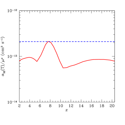
Figure 1.— Average of the recombination to H $\scriptstyle\rm I$ coefficient over the electron contribution to the mean molecular weight, $\mu^{\rm e}$, over H $\scriptstyle\rm II$ regions as a function of $z$ for the temperature evolution shown in Figure 2 (solid red line), obtained from the galaxy model by Manrique et al. (2015) for realistic values of the parameters leading to double hydrogen reionization Salvador-Solé & Manrique (2014), compared to the usual value for a fixed temperature of $10^{4}$ K (dashed blue line).

Besides being better justified than expression (3), expression (5) is also more accurate for the following reasons: i) instead of taking the recombination rate density at a fixed typical temperature divided by $\langle\mu^{\rm e}\rangle_{\rm HII}$, it uses the $z$-dependent average of $\alpha_{\rm HI}(T)/\mu^{\rm e}$ in the H $\scriptstyle\rm II$ region, and ii) the last term on the right accounts for the changing comoving hydrogen density due to inflows/outflows. In Figure 1, we compare $\langle\alpha_{\rm HI}(T)/\mu^{\rm e}\rangle_{\rm HII}$ for the $z$-dependent temperature shown in Figure 2 to the uniform constant value $\alpha_{\rm HI}(T_{\rm typ})/\langle\mu^{\rm e}\rangle_{\rm HII}$ with $T_{\rm typ}=10^{4}$ K appearing in equation (3). As can be seen, the difference is noticeable, particularly around the redshifts $z=$ 10.3 and 5.5 of complete ionization in the particular galaxy model with double reionization considered.

When $Q_{\rm HII}$ reaches the value of one and $\langle\dot{N}_{\rm HII}\rangle$ is sufficient to balance recombinations, a period of ionization equilibrium begins in which $Q_{\rm HII}$ stays equal to one. However, if $\langle\dot{N}_{\rm HII}\rangle$ becomes insufficient to keep ionized regions growing (or stable), a recombination will begin. The constant and decreasing values of $Q_{\rm HII}$ in those two regimes are also governed by equation (5), in the former case with $\langle\dot{N}_{\rm HII}\rangle$ replaced by the equilibrium value, with the leftover metagalactic emissivity eventually used, duly redshifted, to ionize more hydrogen atoms at lower $z$’s.

A similar derivation leads to the homologous equation for the He $\scriptstyle\rm III\$volume filling factor,

$$\frac{{\rm d}Q_{\rm HeIII}}{{\rm d}t}=\frac{\langle\dot{N}_{\rm HeIII}\rangle}{\langle n_{\rm He}\rangle}~{}~{}~{}~{}~{}~{}~{}~{}~{}~{}~{}~{}~{}~{}~{}~{}~{}~{}~{}~{}~{}~{}~{}~{}~{}~{}~{}~{}~{}~{}~{}~{}~{}~{}~{}~{}~{}~{}~{}~{}~{}$$ (6)

$$-\left[\left\langle\frac{\alpha_{\rm HeII}(T)}{\mu^{\rm e}a^{3}}\right\rangle_{\rm III}C_{\rm HII}\,\langle n\rangle+\!\frac{{\rm d}\!\ln\langle n_{\rm He}\rangle}{{\rm d}t}\right]\!Q_{\rm HeIII}\,.$$

Again, if at any point a period of He $\scriptstyle\rm III\$ionization equilibrium or recombination takes place, then $Q_{\rm HeIII}$ stays equal to one or begins to diminish, respectively, according to the same equation (6).

3. Temperature Equations

Photo-ionization leads to photo-heating of the different IGM phases. Other heating mechanisms acting on the IGM are Compton heating by X-rays and by cosmic microwave background (CMB) photons at very high-$z$ (after decoupling of baryons from radiation at $z\sim 150$). Such heating is partially balanced by the cooling due to recombinations and desexcitations, cosmic expansion, Comptonization from CMB photons at low $z$, and collisional cooling (significant only in very hot neutral regions, if any). In addition, density fluctuations suffer gravitational contraction/expansion causing extra heating/cooling. These are the main mechanisms causing the thermal evolution of the IGM. Below we mention (in italics) a few additional mechanisms that are included in the present more accurate treatment (see also Hui & Gnedin 1997 for other possible heating and ionizing mechanisms, due to decaying or annihilating dark matter, not included herein).

The local temperature of the IGM evolves according to the differential equation (e.g. Choudhury & Ferrara 2005)

$$\frac{{\rm d}T}{{\rm d}\ln(1+z)}=T\Big{[}2+\frac{2}{3}\frac{{\rm d}\ln(n/\langle n\rangle_{\rm i})}{{\rm d}\ln(1+z)}~{}~{}~{}~{}~{}~{}$$

$$+\frac{{\rm d}\ln\mu}{{\rm d}\ln(1+z)}+\frac{{\rm d}\ln\varepsilon}{{\rm d}\ln(1+z)}-\frac{{\rm d}\ln n}{{\rm d}\ln(1+z)}\Big{]}.$$ (7)

The first term in claudators on the right, equal to 2, gives the cosmological adiabatic cooling of the gas element; the second term gives its adiabatic heating/cooling by gravitational compression/expansion for the baryon density $n$ around the mean value $\langle n\rangle_{\rm i}$ in region i, taking into account that most diffuse IGM is in a linear or moderately non-linear regime; the third term gives the cooling due to the increase in mean molecular weight, $\mu$, caused by ionization and outflows from halos; the fourth term gives the Compton cooling from CMB photons, and the gain/loss of energy density, $\varepsilon$, due to photo-ionization/recombination, Compton heating from X-rays, the achievement of energy equipartition by newly ionized/recombined fraction of gas (the different phases have distinct temperatures in general) plus mechanical heating accompanying outflows from halos; and the fifth term gives the cooling/heating by the gain/loss of baryon density, $n$, due to outflows/inflows (this changes the average specific energy of the IGM). As outflows take place from halos harboring luminous sources, we assume that they only affect ionized regions.

Multiplying equation (7) by $\mu\,n$, and taking the average over each specific phase under the approximation, for the reasons mentioned in Section 2, that $\mu$, $\varepsilon$, $n$, and $T$ do not correlate with each other, we arrive at

$$\frac{{\rm d}\ln\langle T\rangle_{\rm i}}{{\rm d}\ln(1+z)}=2+\frac{{\rm d}\ln(\langle\mu\rangle_{\rm i}\langle\varepsilon\rangle_{\rm i}/\langle n\rangle_{\rm i})}{{\rm d}\ln(1+z)}\,,$$ (8)

with i=I, II, or III. Note that, in neutral regions (i=I), there are no stochastic effects of luminous sources: $\varepsilon$ does not change either through photo-ionization or by X-rays, $\mu$ is kept strictly equal to the primordial value, and there is only a small change in $n$ due to inflows. Consequently, a strong correlation is foreseen between the quantities $\varepsilon$ and $n$ and temperature. Yet, we still ignore such a correlation for simplicity. This approximation is only necessary during the initial period of increasing ionization; in recombination periods, the gas properties in the new neutral phase remain uncorrelated as they have suffered important stochastic feedback effects from luminous objects over the previous ionized phase.

And what about the temperature dispersion around the mean in the different IGM phases, also required in equations (5) and (6)? To calculate ${\sigma^{2}_{\rm T}}_{i}=\langle T^{2}\rangle_{i}-\langle T\rangle^{2}_{i}$ we need to consider the relation

$$\frac{\frac{1}{2}{\rm d}T^{2}}{{\rm d}\ln(1+z)}\!=\!T^{2}\!\left[2+\frac{2}{3}\frac{{\rm d}\ln(n/\langle n\rangle_{\rm i})}{{\rm d}\ln(1+z)}\!+\!\frac{{\rm d}\ln(\mu\varepsilon/n)}{{\rm d}\ln(1+z)}\right]$$ (9)

following from equation (7). The same steps above lead to

$$\frac{{\rm d}\ln\langle T^{2}\rangle_{\rm i}^{1/2}}{{\rm d}\ln(1+z)}\!=\!2+\frac{{\rm d}\ln(\langle\mu\rangle_{\rm i}\langle\varepsilon\rangle_{\rm i}/\langle n\rangle_{\rm i})}{{\rm d}\ln(1+z)}=\frac{{\rm d}\ln\langle T\rangle_{\rm i}}{{\rm d}\ln(1+z)}.$$ (10)

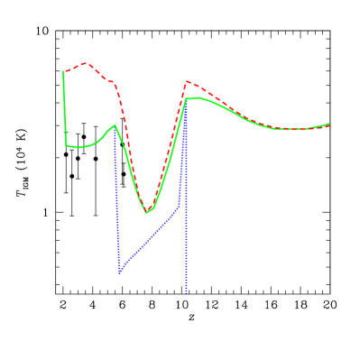
Figure 2.— Average IGM temperatures in neutral (blue dotted lines), singly ionized (green solid lines), and doubly ionized (red dashed lines) regions obtained from the same model with double hydrogen reionization (at $z=10.3$ and 5.5) and single helium reionization (at $z=2$) as in Figure 1. Solid circles with error bars are the actual IGM temperatures estimated by Lidz et al. (2010) and (Bolton et al., 2010, 2012).

The initial conditions for equation (8) are $\langle T\rangle_{\rm I}(z_{\rm ini})=T_{\rm CMB}(z_{\rm ini})$ and $\langle T\rangle_{\rm II}(z_{\rm ini})=\langle\mu\rangle_{\rm II}\langle T\rangle_{\rm I}(z_{\rm ini})/\langle\mu\rangle_{\rm I}$, where $z_{\rm ini}$ is the redshift at which the IGM temperature begins to deviate from the temperature of CMB photons, satisfying $1+z_{\rm ini}=100({\Omega_{\rm b}}h^{2}/0.0125)^{2/5}$, where ${\Omega_{\rm b}}$ and $h$ are the baryonic density parameter and the Hubble parameter scaled to 100 km s^-1 Mpc^-1. Similarly, the initial condition for equation (10) is $\langle T^{2}\rangle_{\rm II}(z_{\rm ini})=\langle\mu\rangle_{\rm II}^{2}\langle T^{2}\rangle_{\rm I}(z_{\rm ini})/\langle\mu\rangle_{\rm I}^{2}$, where $\langle T^{2}\rangle_{\rm I}(z_{\rm ini})$ is equal to ${\sigma^{2}_{\rm T}}_{\rm CMB}(R_{\rm J},z_{\rm ini})+T_{\rm CMB}^{2}(z_{\rm ini})$, where ${\sigma^{2}_{\rm T}}_{\rm CMB}(z_{\rm ini})=2T_{\rm CMB}^{2}(z_{\rm ini})\sigma_{0}(R_{\rm J},z_{\rm ini})^{2}/3$ is the CMB temperature variance at the Jeans scale at recombination, $R_{\rm J}$, evolved to $z_{\rm ini}$, with $\sigma_{0}(R,z)$ the 0-order spectral moment at the scale $R$ and redshift $z$. The reason for the filtering at the scale $R_{\rm J}$ is that, at smaller scales, there were no temperature fluctuations at recombination, and the uniform temperature on those scales only suffered cosmological adiabatic cooling and the effects of luminous sources, uncorrelated with $T$. If there is a period of increasing recombination, the initial mean temperature and variance in the recombined region are equal (except for different mean molecular weights) to those in the ionized phase giving it rise. We have checked that ${\sigma^{2}_{\rm T}}(\langle T\rangle_{\rm i})$ is always much less than $\langle T\rangle^{2}_{\rm i}$, meaning that the second order Taylor expansion around $\langle T\rangle_{\rm i}$ of any arbitrary function $f$ of temperature is really close to the value $f(T)$.

In Figure 2, we show the temperature evolution that results from the present improved treatment of IGM evolution for the source functions, $\dot{N}_{\rm HI}$, $\dot{N}_{\rm HeIII}$, ${\rm d}\ln\langle\varepsilon\rangle_{\rm i}/{\rm d}\ln(1+z)$ and ${\rm d}\ln\langle n\rangle_{\rm i}{\rm d}\ln(1+z)$, provided by the same galaxy model as in Figure 1.

4. Halo Ionization-Bias

The chance that halos with a given mass $M$ at $t$ will trap gas, and that the trapped gas will cool either through molecular bands or atomic lines and form metal-poor or metal-rich stars, respectively, depends on the temperature and ionization state of the IGM in which the halos are embedded. Consequently, the halo MF itself must vary between neutral and ionized environments. Note that, given the homogeneity of the Universe, these probabilities are not a function of a specific point. In particular, the probability that a given arbitrary point lies in a ionized or neutral region is uniform and equal to $Q_{\rm HII}(t)$ and $1-Q_{\rm HII}(t)$, respectively.

To calculate the probability that a halo with mass $M$ is located in an ionized region at the cosmic time $t$, $P_{M}(\hbox{H\hskip 1.5pt$\scriptstyle\rm II$},t)$, we will first consider the conditional probabilities $P_{M}(\hbox{H\hskip 1.5pt$\scriptstyle\rm II$},t|\hbox{H\hskip 1.5pt$\scriptstyle\rm II$},t_{\rm f})$ and $P_{M}(\hbox{H\hskip 1.5pt$\scriptstyle\rm II$},t|\hbox{H\hskip 1.5pt$\scriptstyle\rm I$},t_{\rm f})$ that the halo is in an ionized region at $t$ given that it was either in an ionized or neutral region, respectively, at its formation at $t_{\rm f}$. The former of these two quantities is simply

$$P_{M}(\hbox{H\hskip 1.5pt$\scriptstyle\rm II$},t|\hbox{H\hskip 1.5pt$\scriptstyle\rm II$},t_{\rm f})=1-P_{\rm HI}(t,t_{\rm f})\,,$$ (11)

where $P_{\rm HI}(t,t_{\rm f})$ is the probability that the halo environment recombines between $t_{\rm f}$ and $t$ because of the absence of nearby sufficiently luminous sources. The latter is given by

$$P_{M}(\hbox{H\hskip 1.5pt$\scriptstyle\rm II$},t|\hbox{H\hskip 1.5pt$\scriptstyle\rm I$},t_{\rm f})=P^{\star}_{M}(t,t_{\rm f})+P_{\rm HII}(t,t_{\rm f})\,,$$ (12)

where $P^{\star}_{M}(t,t_{\rm f})$ is the probability that star formation begins to take place in a halo with $M$ lying in a neutral environment between $t_{\rm f}$ and $t$ (we say “begins” because newborn stars soon ionize the medium around the halo), and $P_{\rm HII}(t,t_{\rm f})$ is the probability that the halo environment will become ionized in the same period of time because of the presence of nearby external ionizing sources.

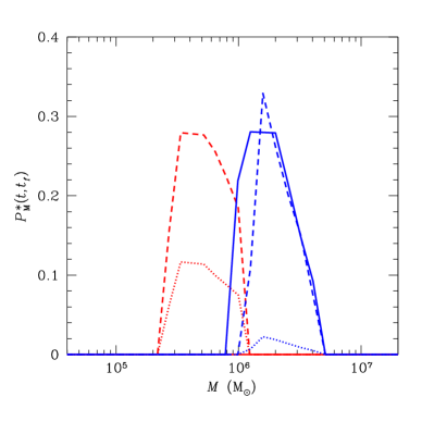
Figure 3.— Probability that star formation will begin to take place in halos with $M$ at $z=15$ (blue lines on the right) and 30 (red lines on the left), before $100$ Myr (solid curves), $30$ Myr (dashed curves), and $10$ Myr (dotted curves) after their formation in neutral regions. Note that at $z=30$ there are not yet any halos $100$ Myr old.

To derive equations (11) and (12) we have assumed that the probabilities $P_{\rm HI}(t,t_{\rm f})$ and $P_{\rm HII}(t,t_{\rm f})$ are independent of halo mass. This may not be the case if there is some correlation between the halo mass- and ionization-biases. However, in terms of the effect of density on the ionization state of a region the tendency for halos harboring more powerful ionizing sources to lie in higher-density regions contrasts with that for ionized bubbles to stretch more rapidly in lower-density regions, so they tend to balance one another. Therefore, even though the importance of this correlation is hard to assess without performing accurate hydrodynamic simulations with ionizing radiative transfer, we do not expect it to be too marked. In other words, the present treatment should be reasonably approximate.

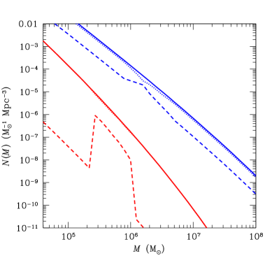
Figure 4.— Halo MF in ionized environments (dashed line) and neutral ones (dotted line) at $z=15$ (blue lines on the right) and 30 (red lines on the left), compared to the global MF (solid line) at the same redshifts, obtained for the same realistic galaxy model as in previous Figures. The higher abundance in ionized environments of halos in a narrow range of low masses is due to the formation of new Population III stars in neutral regions. The rest of the halos in ionized regions arise from the ionization the previous objects produce around them.

The total probability of finding a halo ionized at $t$ can be expressed in terms of the above conditional probabilities and $P_{M}(\hbox{H\hskip 1.5pt$\scriptstyle\rm II$},t)$ upon formation,

$$P_{M}(\hbox{H\hskip 1.5pt$\scriptstyle\rm II$},t)=P_{M}(\hbox{H\hskip 1.5pt$\scriptstyle\rm II$},t|\hbox{H\hskip 1.5pt$\scriptstyle\rm II$},t_{\rm f})P_{M}(\hbox{H\hskip 1.5pt$\scriptstyle\rm II$},t_{\rm f})$$

$$+P_{M}(\hbox{H\hskip 1.5pt$\scriptstyle\rm II$},t|\hbox{H\hskip 1.5pt$\scriptstyle\rm I$},t_{\rm f})\left[1-P_{M}(\hbox{H\hskip 1.5pt$\scriptstyle\rm II$},t_{\rm f})\right]\,.$$ (13)

Substituting the conditional probabilities on the right of equation (13) by expressions (11) and (12), setting $t=t_{\rm f}+\Delta t$, and taking the limit of small $\Delta t$, equation (13) leads to the following differential equation governing the evolution of $P_{M}(\hbox{H\hskip 1.5pt$\scriptstyle\rm II$},t)$

$$\frac{{\rm d}P_{M}(\hbox{H\hskip 1.5pt$\scriptstyle\rm II$},t)}{{\rm d}t}=\frac{{\rm d}Q_{\rm HII}(t)}{{\rm d}t}+\frac{{\rm d}P^{\star}_{M}(t,t_{\rm f})}{{\rm d}t}\left[1-Q_{\rm HII}(t)\right]\,.$$ (14)

To derive equation (14) we have taken $P_{\rm HI}(t,t_{\rm f})=0$ and $P_{\rm HII}(t,t_{\rm f})=[Q_{\rm HII}(t)-Q_{\rm HII}(t_{\rm f})]/[1-Q_{\rm HII}(t_{\rm f})]$ in periods of increasing ionization, and $P_{\rm HI}(t,t_{\rm f})=[Q_{\rm HII}(t_{\rm f})-Q_{\rm HII}(t)]/Q_{\rm HII}(t_{\rm f})$ and $P_{\rm HII}(t,t_{\rm f})=0$, in periods of increasing recombination. Interestingly, in both cases one is led to the same differential equation (14), whose solution for the initial condition $P_{M}(\hbox{H\hskip 1.5pt$\scriptstyle\rm II$},0)=0$ yields the desired probability $P_{M}(\hbox{H\hskip 1.5pt$\scriptstyle\rm II$},t)$ of finding a halo with $M$ in a ionized region at $t$, its complementary value giving the probability $P_{M}(\hbox{H\hskip 1.5pt$\scriptstyle\rm I$},t)$ of finding it in a neutral region.

The probability $P^{\star}_{M}(t,t_{\rm f})$ in equation (14) is hard to estimate analytically because it depends on the number fraction of H₂ molecules, $f_{\rm H_{2}}$, at the center of halos with $M$, whose PDF cannot be established without making appeal to the whole halo aggregation history. Thus, this function must be drawn from a full treatment of galaxy and IGM evolution. In Figure 3, we plot this function obtained from the same galaxy model as in previous Figures. The halo MFs in ionized and neutral regions resulting from a global MF of the Sheth & Tormen (2002) form at two different redshifts are plotted in Figure 4. As can be seen, the higher the redshift, the more marked the effect,which is only visible, of course, before full ionization.

5. SUMMARY

In the present paper, we have derived an improved version of the master equations for the evolution of IGM ionization state and temperature, accounting for the composite, inhomogeneous, multiphase nature of this medium. Besides all the usual effects, the new version includes collisional cooling in hot neutral regions (necessary to deal with recombination periods as found in double reionization), mass exchanges between halos and IGM, and the achievement equipartition for newly ionized/recombined gas. In addition, we have derived the probability that a halo with a given mass $M$ at $z$ is located in a ionized or neutral environment, which is needed to accurately compute the source functions required in the IGM master equations.

To check the performance of this improved treatment of IGM we coupled it to the galaxy model by Manrique et al. (2015) for realistic values of the parameters leading to double reionization (Salvador-Solé & Manrique, 2014). The main results were as follows:

- The average temperatures in the three IGM phases show marked variations over the different ionization/recombination periods. This harbors relevant information on the epoch of reionization. The usual treatment dealing with the average temperature over the whole IGM (or at mean IGM density, $T_{0}$) loses this information.

- The inclusion of collisional cooling is mandatory to recover the sudden decrement in the average temperature of neutral regions after first ionization in double reionization (see Fig. 2). In the only work to date, by Choudhury & Ferrara (2005), dealing with the evolution of the average temperature in the different IGM phases, neutral regions cooled adiabatically after decoupling.

- The average temperatures of singly and doubly ionized regions show a maximum similar to that found by Choudhury & Ferrara (2005; see panel f of their Fig. 1). However, our temperatures also show a minimum, due to the recombination after first ionization. More importantly, the average temperature in doubly ionized regions is always higher than in singly ionized ones, while this was surprisingly not the case in Choudhury & Ferrara’s solution.

- Although the average temperature in singly ionized regions is not as high as that reported by Choudhury and Ferrara, it is still notably higher (by a factor of $\sim 3$) than the value of $10^{4}$ K often adopted in reionization studies (Shapiro et al., 1994; Wyithe & Loeb, 2003; Benson et al., 2006; Zhang et al., 2007).

- This difference translates into the average recombination coefficients. The values we find are substantially smaller (by a factor $\sim 4$) than found for the temperature of $10^{10}$ K, and somewhat greater (by a factor $\sim 2$) than the minimum value at the average temperature reached in Choudhury & Ferrara’s solution.

- This affects the evolution of the volume filling factors of ionized hydrogen and helium for identical source functions (identical galaxy models). But this makes a small difference compared to that arising from the galaxy models used, which may lead, for instance, to single or double reionization.

- We have computed the halo ionization-bias in the calculation of the source functions appearing in the IGM master equations. The ratios between the halo MF in ionized and all environments found for low mass newly star-forming halos and for the rest are respectively equal to $\sim 3\times 10^{-4}$ ($0.1$) and $\sim 0.3$ ($0.4$) at $z=30$ ($z=15$).

This improved treatment of IGM can be easily implemented in any model of galaxy and IGM evolution. This is particularly advisable for accurate models of galaxy formation or reionization when contrasting them with current observations (e.g. Salvador-Solé & Manrique 2014) or future ones (e.g. 21 cm line experiments).

References

- Alvarez et al. (2012) Alvarez, M. A., Finlator, K., & Trenti, M. 2012, ApJ, 759, L38
- Battaglia et al. (2013) Battaglia, N., Trac, H., Cen, R., & Loeb, A. 2013, ApJ, 776, 81
- Babul & Rees (1992) Babul, A., & Rees, M. J. 1992, MNRAS, 255, 346
- Benson et al. (2006) Benson, A. J., Sugiyama, N., Nusser, A., & Lacey, C. G. 2006, MNRAS, 369, 1055
- Bolton et al. (2010) Bolton, J. S., Becker, G. D., Wyithe, J. S. B., Haehnelt, M. G., & Sargent, W. L. W. 2010, MNRAS, 406, 612
- Bolton et al. (2012) Bolton, J. S., Becker, G. D., Raskutti, S., et al. 2012, MNRAS, 419, 2880 bf
- Bower et al. (2006) Bower, R. J., Benson, A. J., Malbon, R., Helly, J. C., Frenk, C. S., Baugh, C. M., Cole, S., & Lacey, C. G. 2006, MNRAS, 370, 645
- Choudhury & Ferrara (2005) Choudhury, T. R., & Ferrara, A. 2005, MNRAS, 361, 577
- Ciardi et al. (2000) Ciardi, B., Ferrara, A., Governato, F., & Jenkins, A. 2000, MNRAS, 314, 611
- Cole (1991) Cole, S. 1991, ApJ, 367, 45
- Croton et al. (2006) Croton, D. J., et al. 2006, MNRAS, 365, 11
- Dekel & Silk (1986) Dekel, A. & Silk, J. 1986, 303, 39
- Dijkstra et al. (2004) Dijkstra, M., Haiman, Z., Rees, M. J., & Weinberg, D. H. 2004, ApJ, 601, 666
- D’Odorico et al. (2013) D’Odorico, V., et al. 2013, MNRAS, 435, 1198
- Efstathiou (1992) Efstathiou, G. 1992, MNRAS, 256, 43P
- Faucher-Giguère et al. (2009) Faucher-Giguère, C.-A., Lidz, A., Zaldarriaga, M., & Hernquist, L. 2009, ApJ, 703, 1416
- Finlator et al. (2012) Finlator, K., Oh, S. P., Özel, F., & Davé, R. 2012, MNRAS, 427, 2464
- Font et al. (2011) Font, A. S., Benson, A. J., Bower, R. G., et al., 2011 MNRAS, 417, 1260
- Furlanetto et al. (2004) Furlanetto, S. R., Zaldarriaga, M., & Hernquist, L. 2004, ApJ, 613, 1
- Haiman et al. (1996) Haiman, Z., Thoul, A. A., & Loeb, A. 1996, ApJ, 464, 523
- Haiman & Holder (2003) Haiman, Z., & Holder, G. 2003, ApJ, 595, 1
- Hui & Gnedin (1997) Hui, L., & Gnedin, N. Y. 1997, MNRAS, 297, 27
- Hui & Haiman (2003) Hui, L., & Haiman, Z. 2003, ApJ, 596, 9
- Iliev et al. (2007) Iliev, I. T., Mellema, G., Shapiro, P. R., & Pen, U.-L. 2007, MNRAS, 376, 534
- Ikeuchi (1986) Ikeuchi, S. 1986, ApJSS, 118, 509
- Kaurov & Gnedin (2013) Kaurov, A. A., & Gnedin, N. Y. 2013, ApJ, 771, 35
- Lacey & Silk (1991) Lacey, C. G. & Silk, J. 1991, ApJ, 381, 14
- Lidz et al. (2010) Lidz, A., Faucher-Giguère, C.-A., Dall’Aglio, A., et al. 2010, ApJ718, 199
- Manrique et al. (2015) Manrique, A., Salvador-Solé, E., Juan, E., Hatziminaoglou, E., E., Rozas, J. M., Sagristà, A., Casteels, K., J., Bruzual, G., Magris, G. 2015, ApJS, 216, 13
- Meiksin (2009) Meiksin, A. A. 2009, Reviews of Modern Physics, 81, 1405
- Mesinger & Dijkstra (2008) Mesinger, A., & Dijkstra, M. 2008, MNRAS, 390, 1071
- Miralda-Escudé & Ostriker (1990) Miralda-Escudé, J., & Ostriker, J. P. 1990, ApJ, 350, 1
- Miralda-Escudé & Ostriker (1992) Miralda-Escudé, J., & Ostriker, J. P. 1992, ApJ, 392, 15
- Miralda-Escudé & Ostriker (1994) Miralda-Escudé, J., & Ostriker, J. P. 1994, MNRAS, 266, 343
- Miralda-Escudé & Rees (1994) Miralda-Escudé, J., & Rees, M. J. 1994, MNRAS, 266, 343
- Miralda-Escudé, Haehnelt, & Rees (2000) Miralda-Escudé, J., Haehnelt, M., & Rees, M. J. 2000, ApJ, 530, 1
- Navarro & Steinmetz (1997) Navarro, J., & Steinmetz, M. 1997, ApJ, 478, 13
- Oh & Haiman (2003) Oh, S. P., & Haiman, Z. 2003, MNRAS, 332, 59
- Okamoto et al. (2008) Okamoto, T., Gao, L., & Theuns, T. 2008, MNRAS, 390, 920
- Quinn, Katz, & Efstathiou (1996) Quinn, T., Katz, N., & Efstathiou, G. 1996, MNRAS, 278, L49
- Rees (1986) Rees, M. J. 1986, MNRAS, 218, 25P
- Salvador-Solé & Manrique (2014) Salvador-Solé, E., & Manrique, A. 2014, in progress
- Shapiro et al. (1990) Shapiro, P. R., Giroux, M. L., & Babul, A. 1990 in After the First Three Minutes, ed. S. Holt, V. Trimble, & C. Bennett AIP Conf. Proc. 222), 347
- Shapiro et al. (1994) Shapiro, P. R., Giroux, M. L., & Babul, A. 1994, ApJ, 427, 25
- Shapiro & Giroux (1987) Shapiro, P. R., & Giroux, M. L. 1987, ApJ, 321, L07
- Sheth & Tormen (2002) Sheth R. K., & Tormen G., 2002, MNRAS, 329, 61
- Simcoe et al. (2011) Simcoe, R. A., Cooksey, K. L., Matejek, M., et al. 2011, ApJ, 743, 21
- Sobacchi & Mesinger (2013a) Sobacchi, E., & Mesinger, A. 2013a, MNRAS, 432, 51
- Sobacchi & Mesinger (2013b) Sobacchi, E., & Mesinger, A. 2013b, MNRAS, 432, 3340
- Trac et al. (2008) Trac, H., Cen, R., & Loeb, A. 2008, ApJ, 689, L81
- Thoul & Weinberg (1996) Thoul, A. A., & Weibnberg, D. H. 1996, ApJ, 465, 608
- Tinker et al. (2010) Tinker, J. L., Robertson, B. E., Kravtsov, A. V., et al. 2010, ApJ, 724, 878
- White & Rees (1978) White, S. D. M., & Rees, M. 1978, MNRAS, 183, 341
- White & Frenk (1991) White, S. D. M., & Frenk, C. S. 1991, ApJ, 379, 52
- Weinberg, Hernquist, & Katz (1997) Weinberg, D. H., Hernquist, L., & Katz, N. 1997, ApJ, 477, 8
- Wyithe & Loeb (2003) Wyithe, J. S. B., & Loeb, A. 2003, ApJ, 586, 693
- Wyithe & Loeb (2013) Wyithe, J. S. B., & Loeb, A. 2013, MNRAS, 428, 2741
- Zhang et al. (2007) Zhang, J., Hui, L., & Haiman, Z. 2007, MNRAS, 375, 324
- Zahn et al. (2011) Zahn, O., Mesinger, A., McQuinn, M, et al. 2011, MNRAS, 414, 727
- Zhou et al. (2013) Zhou, J., Guo, Q., Liu, G.-C. et al. 2013, RAA, 13, 373