Abstract: Feature modeling is a widely used formalism to characterize a set of products (also called configurations). As a manual elaboration is a long and arduous task, numerous techniques have been proposed to reverse engineer feature models from various kinds of artefacts. But none of them synthesize feature attributes (or constraints over attributes) despite the practical relevance of attributes for documenting the different values across a range of products. In this report, we develop an algorithm for synthesizing attributed feature models given a set of product descriptions. We present sound, complete, and parametrizable techniques for computing all possible hierarchies, feature groups, placements of feature attributes, domain values, and constraints. We perform a complexity analysis w.r.t. number of features, attributes, configurations, and domain size. We also evaluate the scalability of our synthesis procedure using randomized configuration matrices. This report is a first step that aims to describe the foundations for synthesizing attributed feature models.

Key-words: Attributed feature models, Product descriptions, Reverse engineering

Synthèse de Modèles de Caractéristiques Attribués à Partir de Descriptions de Produits : Fondations

Résumé : La modélisation de caractéristiques (features) est un formalisme largement utilisé pour décrire un ensemble de produits (ou configurations). Comme une élaboration manuelle est une tâche longue et ardue, de nombreuses techniques ont été proposées pour extraire des modèles de caractéristiques à partir de types variés d’artefacts. Aucune d’elles cependant ne considère la synthèse d’attributs de caractéristiques (ou de contraintes portant sur les attributs) malgré l’utilité pratique des attributs pour documenter différentes valeurs d’un ensemble de produits. Dans ce rapport, nous développons un algorithme pour synthétiser des modèles de caractéristiques attribués, étant donné un ensemble de descriptions de produits. Nous présentons des techniques correctes, complètes et paramétrables pour calculer toutes les hiérarchies possibles, groupes de caractéristiques, placements d’attributs, valeurs de domaines et contraintes. Nous effectuons une analyse de complexité par rapport au nombre de caractéristiques, d’attributs, de configurations et de la taille des domaines. Nous évaluons aussi le passage à l’échelle de notre procédure de synthèse en utilisant des matrices de configurations générées aléatoirement. Ce rapport est une première étape qui vise à décrire les fondations pour synthétiser des modèles de caractéristiques attribués.

Mots-clés : Modèle de caractéristiques, Description de produits, Rétro-ingénierie

1 Introduction

Configuration options are ubiquitous. They allow users to customize or choose their product. Options (also referred as features or attributes) refer to functional and non-functional aspects of a system, at different level of granularity – from parameters in a function to a whole service. For example, software practitioners can activate or deactivate some functionalities and tune the energy consumption and memory footprint when building a product for embedded systems. Customers themselves can select a set of desired options to match their requirements – for satisfying their functional needs without e.g. reaching a maximum budget.

Modeling features or attributes of a given set of products is a crucial activity in Software Product Line (SPL) engineering. The formalism of feature models (FMs) is widely employed for this purpose [1, 2, 3, 4]. FMs delimit the scope of a family of related products (i.e., an SPL) and formally document what combinations of features are supported. Once specified, FMs can be used for model checking an SPL [5, 6, 7, 8], automating product configuration [9, 10, 11, 12], computing relevant information [13] or communicating with stakeholders [14]. In many generative or feature-oriented approaches, FMs are also central for deriving software-intensive products [15].

Feature attributes are a useful extension, intensively employed in practice, for documenting the different values across a range of products [16]. With the addition of attributes, optional behaviour can be made dependent not only on the presence or absence of features, but also on the satisfaction of constraints over domain values of attributes [6]. Recently, languages and tools have emerged to fully support attributes in feature modeling and SPL engineering (e.g., see [13, 17, 18, 19, 20, 21, 22, 23, 24, 25, 26, 12, 27]).

The manual elaboration of a feature model – being with attributes or not – is known to be a daunting and error-prone task [28, 29, 30, 31, 32, 33, 34, 35, 36, 37, 38, 39, 3, 31, 40, 41, 42, 43, 44, 45, 46, 47, 41, 48, 49]. The number of features, attributes, and dependencies among them can be very important so that practitioners can face severe difficulties for accurately modeling a set of products. In response, numerous synthesis techniques have been developed for synthesising feature models [3, 31, 40, 41, 42, 43, 44, 45, 46, 47, 41, 48, 49]. Until now, the impressive research effort has focused on synthesizing basic, Boolean feature models – without feature attributes. Despite the evident opportunity of encoding quantitative information as attributes, the synthesis of attributed feature models has not yet caught attention. None of the existing techniques synthesize feature attributes, domain values or constraints over attributes.

In this report, we develop the theoretical foundations and techniques for synthesizing attributed feature models given a set of product descriptions. We present sound, complete, and parametrizable techniques for computing hierarchies, feature groups, placements of feature attributes, domain values, and constraints. We describe algorithms for computing logical relations between features and attributes. The synthesis is capable of taking knowledge (e.g., about the hierarchy and placement of attributes) into account so that users can specify, if needs be, a hierarchy or some placements of attributes.

We perform a complexity analysis of our synthesis procedure with regards to the number of configurations, features, attributes, and domain values. We also evaluate the scalability of the synthesis using randomized configuration matrices. Our work both strengthens the understanding of the formalism and provides the basis of a tool-supported solution for synthesizing attributed feature models.

The foundations presented in this report open avenues for investigating novel reverse engineering scenarios involving attributes. Numerous works have developed techniques for mining and extracting features or constraints from various kinds of artefacts [28, 29, 30, 31, 32, 33, 34, 35, 36, 37, 38, 39] (textual requirements, design models, source code, semi-structured or informal product descriptions, configurators, etc.). However, they do not support attributes despite the presence of non Boolean data in some of these artefacts. Such automated extraction techniques can be used to process different types of artefacts and eventually fed our synthesis algorithm.

The remainder of the report is organized as follows. Section 2 discusses related work. Section 3 further motivates the need of synthesising attributed FMs. Section 4 exposes the problem of synthesizing attributed FMs. Section 5 presents our algorithm targeting this problem. Section 6 and  7 respectively evaluate the synthesis techniques from a theoretical and practical aspect. In Section 8 we discuss threats to validity. Section 9 summarizes the contributions and describes future work.

2 Related Work

Numerous works address the synthesis or extraction of FMs. Despite the availability of some tools and languages supporting attributes, no prior work consider the synthesis of attributed FMs. They solely focus on Boolean FMs.

2.1 Synthesis of Feature Models

Techniques for synthesising an FM from a set of dependencies (e.g., encoded as a propositional formula) or from a set of configurations (e.g., encoded in a product comparison matrix) have been proposed [3, 31, 40, 41, 42, 43, 44, 45, 46].

In [3, 45, 47], the authors calculate a diagrammatic representation of all possible FMs from a propositional formula (CNF or DNF). In [41], we propose a synthesis procedure that processes user-specified knowledge for organizing the hierarchy of features. In [48], we also propose a set of techniques for synthesizing FMs that are both correct w.r.t input propositional formula and present an appropriate hierarchy.

The algorithms proposed in [42, 44, 43, 49] take as input a set of configurations. The generated FM may not conform to the input configurations, that is, the FM may be an over-approximation of the configuration set. Our work aims to study whether similar properties arise in the context of attributed feature models. The approaches presented in [42, 44, 43, 49] do not control the way the FM hierarchy is synthesized. The major drawback is that the resulting hierarchy is likely to be difficult to read, understand, and exploit [48, 50]. In contrast, She et al. [31] proposed a heuristic to synthesize an FM presenting an appropriate hierarchy. Applied on the software projects Linux, eCos, and FreeBSD, the technique assumes the existence of feature descriptions. Janota et al. [40] developed an interactive editor, based on logical techniques, to guide users in synthesizing an FM from a propositional formula. In prior works [48, 50, 41], we develop techniques for taking the so-called ontological semantics into account when synthesizing feature models. Our work shares the goal of interactively supporting users – this time in the context of synthesizing attributed feature models.

Overall, numerous works exist for the synthesis of FMs but none support attributes.

2.2 Extraction of Feature Models

Considering a broader view, reverse engineering techniques have been proposed to extract FMs from various artefacts.

Davril et al. [28] presented a fully automated approach, based on prior work [51], for constructing FMs from publicly available product descriptions found in online product repositories and marketing websites such as SoftPedia and CNET. In [29], a semi-automated procedure to support the transition from product descriptions (expressed in a tabular format) to FMs is proposed. In [30], architectural knowledge, plugins dependencies and the slicing operator are combined to obtain an exploitable and maintainable FM. Ryssel et al. developed methods based on Formal Concept Analysis and analyzed incidence matrices containing matching relations [32].

Yi et al. [52] proposed to apply support vector machine and genetic techniques to mine binary constraints (requires and excludes) from Wikipedia. This scenario is particularly relevant when dealing with incomplete dependencies. They evaluated their approach on two FMs of SPLOT. Bagheri et al. [33] proposed a collaborative process to mine and organize features using a combination of natural language processing techniques and Wordnet. Ferrari et al. [34] applied natural language processing techniques to mine commonalities and variabilities from brochures. Alves et al. [35], Niu et al. [36], Weston et al. [37] and Chen et al. [38] applied information retrieval techniques to abstract requirements from existing specifications, typically expressed in natural language.

Another related subject is constraint mining. In [30], architectural and expert knowledge as well as plugins dependencies are combined to obtain an exploitable and maintainable feature model. Nadi et al. [39] developed a comprehensive infrastructure to automatically extract configuration constraints from C code.

All these works present innovative techniques for mining and extracting FMs from various artefacts. However, they do not support the synthesis of attributes despite the presence of non Boolean data in some of these artefacts. In this report, we do not consider such a broad view; we focus solely on the synthesis of AFMs. Automated extraction techniques can be used to process different types of artefacts and eventually fed our synthesis algorithm. The foundations presented in this report open avenues for investigating novel reverse engineering scenarios involving attributes.

2.3 Language and Tool Support for Feature Models

There are numerous existing academic (or industrial) languages and tools for specifying and reasoning about FMs [13, 53].

FeatureIDE [54, 55] is an Eclipse-based IDE that supports all phases of feature-oriented software development. SPLConqueror is a tool to measure and optimize non-functional properties in software product lines [21, 22, 23]. Descriptions of product lines include feature attributes such as pricing, footprint etc.

FAMA (Feature Model Analyser) [13] is a framework for the automated analysis of FMs integrating some of the most commonly used logic representations and solvers. It supports attributes with integer, real and string domains. SPLOT [56] provides a Web-based environment for editing and configuring FMs. S2T2 [57] is a tool for the configuration of large FMs. Commercial solutions (pure::variants [58] and Gears [59]) also provide a comprehensive support for product lines (from FMs to model/source code derivation). TVL [18] is a language supporting several extensions to FMs such as attributes. Clafer [19] is a framework mixing feature models and meta-models that supports the definition and analysis of attributes. Seidl et al. [20] propose an extension of FMs for supporting variability in time and space. The so-called hyper FMs can be considered as a special case of AFMs in which attributes’ domains are graphs of version. Alferez et al. reported an experience in the video domain involving numerous numerical values and meta-information, encoded as attributes with the VM language [27].

None of the existing tools propose support for synthesizing attributed FMs.

3 Background and Motivation

This report aims to describe the foundations for synthesizing an attributed feature model from product descriptions. In this section, we describe background information related to attributed feature models. We then explain why attributes are an essential extension to feature models in order to support the expressiveness of product descriptions. We further motivate the need for an automated encoding of product descriptions.

3.1 Attributed Feature Models

Several formalisms supporting attributes exist [60, 18, 19, 61]. In this report, we use a formalism inspired from FAMA [60]. An AFM is composed of a feature diagram (see Definition 1) and an arbitrary constraint (see Definition  2).

Definition 1 (Attributed Feature Diagram).

An attributed feature diagram FD is a tuple $\langle F$, $H$, $E_{M}$, $G_{MTX}$, $G_{XOR}$, $G_{OR}$, $A$, $D$, $\delta$, $\alpha$, $RC\rangle$ such that:

• $F$ is a finite set of boolean features.

• $H=(F,E)$ is a rooted tree of features where $E\subseteq F\times F$ is a set of directed child-parent edges.

• $E_{M}\subseteq E$ is a set of edges that define mandatory features.

• $G_{MTX},G_{XOR},G_{OR}\subseteq P(E\backslash{}E_{m})$ are sets of feature groups. Each feature group is a set of edges. The feature groups of $G_{MTX}$, $G_{XOR}$ and $G_{OR}$ are non-overlapping and all edges in a group share the same parent.

• $A$ is a finite set of attributes.

• $D$ is a set of possible domains for the attributes in $A$.

• $\delta\in A\rightarrow D$ is a total function that assigns a domain to an attribute.

• $\alpha\in A\rightarrow F$ is a total function that assigns an attribute to a feature.

• $RC$ is a set of constraints over $F$ and $A$ that are considered as human readable and may appear in the feature diagram in a graphical or textual representation (e.g. binary implication constraints can be represented as an arrow between two features).

A domain $d\in D$ is a tuple $\langle V_{d},0_{d},<_{d}\rangle$ with $V_{d}$ a finite set of values, $0_{d}\in V_{d}$ the null value of the domain and $<_{d}$ a partial order on $V_{d}$. When a feature is not selected, all its attributes bound by $\alpha$ take their null value, i.e. $\forall(a,f)\in\alpha\text{ with }\delta(a)=\langle V_{a},0_{a},<_{a}\rangle\text{, we have }\neg f\Rightarrow(a=0_{a})$.

readable_constraint ::= bool_factor ‘$\Rightarrow$’ bool_factor ; bool_factor ::= feature_name $|$ ‘$\neg$’ feature_name $|$ rel_expr ; rel_expr ::= attribute_name rel_op num_literal ; rel_op ::= ‘$>$’ $|$ ‘$<$’ $|$ ‘$\geq$’ $|$ ‘$\leq$’ $|$ ‘=’ ;

Figure 1: The grammar of readable constraints.

For the set of constraints in $RC$, formally defining what is human readable is essential for automated techniques. In this report, we define $RC$ as the constraints that are consistent with the grammar in Figure 1. Some examples of such constraints can be found in the bottom of Figure 2(b). We consider that these constraints are small enough and simple enough to be human readable. In this grammar, each constraint is a binary implication, which specifies a relation between the values of two attributes or features. Feature names and relational expressions over attributes are the boolean factors that can appear in an implication. Further, we only allow natural numbers as numerical literals (num_literal).

The grammar of Figure 1 and the formalism of attributed feature diagrams (see Definition 1) are not expressive enough to represent any possible configuration matrix [62]. Therefore, to exactly represent a configuration matrix, we need to add an arbitraty constraint to the feature diagram. This leads to the definition of an attributed feature model (see Definition 2).

Definition 2 (Attributed Feature Model).

A feature model is a pair $\langle FD,\Phi\rangle$ where FD is an attributed feature diagram and $\Phi$ is an arbitrary constraint over $F$ and $A$ that represent the constraints that cannot be expressed by $RC$.

Example. Figure 2(b) shows an example of an AFM describing a product line of Wiki engines. The feature WikiMatrix is the root of the hierarchy. It is decomposed in 3 features: LicenseType which is mandatory and WYSIWYG and LanguageSupport which are optional. The xor-group composed of GPL, Commercial and NoLimit defines that the wiki engine has exactly 1 license and it must be selected among these 3 features. The attribute LicensePrice is attached to the feature LicenseType. The attribute’s domain states that it can take a value in the following set: {0, 10, 20}. The readable constraints and $\Phi$ for this AFM are listed below its hierarchy (see Figure 2(b)). The first one restricts the price of the license to 10 when the feature Commercial is selected.

As illustrated by the example, an AFM has two main objectives. First, it defines the valid configurations of a product line. This corresponds to the configuration semantics of the AFM (see Definition 3). Second, it organizes the relationships between the features and attributes which can be of different types (e.g. decomposition or specialization). This corresponds to the ontological semantics of the AFM (see Definition 4).

Definition 3 (Configuration semantics).

A configuration of an AFM $m$ is defined as a set of selected features and a value for every attribute. The configuration semantics $\llbracket m\rrbracket$ of $m$ is the set of valid configurations.

Definition 4 (Ontological semantics).

The hierarchy $H$, the feature groups ($G_{MTX}$, $G_{OR}$ and $G_{XOR}$), the place of the attributes defined by $\alpha$ and the constraints $RC$ form the ontological semantics of an attributed feature model. It represents the semantics of features and attributes’ relationships including their structural relationships and conceptual proximity.

3.2 Product Descriptions and Feature Models

Product descriptions are usually represented in tabular format, such as spreadsheets and product comparison matrices. The objective of such formats is to describe the characteristics of a set of products in order to document and differentiate them. From now on, we will use the term configuration matrix to refer to these tabular formats (see Definition 5 for a formal description).

For instance, consider the domain of Wiki engines that we will use as a running example throughout the report. The list of features supported by a set of Wiki engines can be documented using a configuration matrix. Figure 2(a) is a very simplified configuration matrix, which provides information about eight different Wiki engines.

Definition 5 (Configuration matrix).

Let $\mathbf{c}_{1},...,\mathbf{c}_{M}$ be a given set of configurations. Each configuration $\mathbf{c}_{i}$ is an $N$-tuple $(c_{i,1},...,c_{i,N})$, where each element $c_{i,j}$ is the value of a variable $V_{j}$. A variable represents either a feature or an attribute. Using these configurations, we create an $M\times N$ matrix $\mathbf{C}$ such that $\mathbf{C}=[\mathbf{c}_{1},...,\mathbf{c}_{M}]^{t}$, and call it a configuration matrix.

Identifier	LicenseType	LicensePrice	Language	Language	WYSIWYG
			Support
Confluence	Commercial	10	Yes	Java	Yes
PBwiki	NoLimit	20	No	–	Yes
SimpleWiki	NoLimit	10	No	–	Yes
MoinMoin	GPL	0	Yes	Python	Yes
TWiki	GPL	0	Yes	Perl	Yes
PerlWiki	GPL	10	Yes	Perl	Yes
MediaWiki	GPL	0	Yes	PHP	No
PHPWiki	GPL	10	Yes	PHP	Yes

(a) A configuration matrix for Wiki engines.

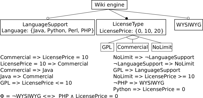
(b) One possible attributed feature model for representing the configuration matrix in Figure 2(a)

Information	Value
Features	WYSIWYG, LanguageSupport, LicenseType, GPL, Commercial, NoLimit
Interpretation of cells	"Yes" = presence of a feature, "No" = absence of a feature
Root	Wiki engine
Hierarchy (child $\rightarrow$ parent)	LanguageSupport $\rightarrow$ Wiki engine, LicenseType $\rightarrow$ Wiki engine, WYSIWYG $\rightarrow$ Wiki engine, GPL $\rightarrow$ LicenseType, Commercial $\rightarrow$ LicenseType, NoLimit $\rightarrow$ LicenseType
Attributes	Language, LicensePrice
Domains	"–" is the null value of Language
Place of attributes	$\alpha(\emph{Language})=\emph{LanguageSupport}$, $\alpha(\emph{LicensePrice})=\emph{LicenseType}$
Feature groups	$\{$GPL, Commercial, NoLimit$\}$
Interesting values for RC	(LicensePrice, 10)

(c) Domain knowledge for synthesizing Figure 2(b) from Figure 2(a).

Figure 2: A motivating example

Conceptually, a configuration matrix documents a family of related products (e.g., an SPL). Feature models can also be used to document a set of configurations (products). Though feature models and configuration matrices share the same goal, their syntax and usage vastly differ.

In contrast to configuration matrices, feature models do not provide an explicit listing (or enumerative definition) of the set of products. From this perspective, feature models are rather a compact representation of a set of products; variability information (e.g., optionality) and cross-tree constraints define the legal configurations corresponding to products. Domain analysts can quickly visualize what are the relationships between features. First, the variability information is made explicit and can be directly read and understood. Moreover the hierarchy helps to structure the information and a potentially large number of features into multiple levels of increasing detail [2]. Besides, an enumerative definition of a set of products is only practical for relatively small sets; feature models are particularly suited when the enumeration of the set is impractical.

Configuration matrices and feature models are semantically related and aim to characterize a set of configurations. The two formalisms are complementary; one would like to switch from one representation to the other.

3.3 Synthesis of Attributed Feature Models

Our first goal is to further the understanding of the relation between the two formalisms (RQ1). Our second goal is to provide synthesis mechanisms to transition from configuration matrices to feature models (RQ2).

More specifically, we want to formalize the relationship between configuration matrices and attributed feature models (RQ1). Previous works [29, 45] limit their study to Boolean constructs. However, non Boolean data (e.g. numbers, strings or dates) are intensively employed in configuration matrices to document variability [63, 64, 65]. For instance, the price of the license is represented by an integer in Figure 2(a). These kinds of data are typically encoded as attributes in a feature model. Figure 2(b) shows an attributed feature model, and a set of constraints that together provide a possible representation of the comparison matrix in Figure 2(a). In the attributed feature model, the feature LicenseType contains an attribute named LicensePrice that represents the price of the license. In general, a configuration matrix can be represented by a multiplicity of feature models. To choose a unique one among them, we use some extra information that we call domain knowledge. The domain knowledge that is used for generating the feature model in Figure 2(b) is shown in Figure 2(c).

With regards to RQ2, numerous works reported that the manual development of a feature model is time-consuming and error-prone [28, 29, 30, 31, 32, 33, 34, 35, 36, 37, 38, 39, 3, 31, 40, 41, 42, 43, 44, 45, 46, 47, 41, 48, 49]. We assist users in synthesizing a consistent and meaningful feature model – this time with attributes.

3.4 Synthesis Scenarios

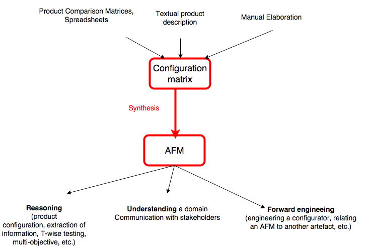
Figure 3: Core problem: synthesis of attributed feature model from configuration matrix

Figure 3 summarizes our objective. On the one hand, many kinds of artefacts or problems are amenable to the formalism of configuration matrix (see on top). Product comparison matrices (PCMs) [63, 64, 65] abound on the internet and are describing products along different criteria. Modulo a fixed and precise interpretation of cell values, PCMs can be encoded as configuration matrices. Our recent initiative for automating the formalization and providing state-of-the-art, specialized editors for PCMs can help for this purpose [65]. Some textual descriptions of product can also be encoded as a configuration matrix [28]. A manual listing of configurations can also be created and maintained. Berger et al. [14] reported that practitioners use FMs to manage a set of configurations. Guo et al. compute similar configuration matrices for assessing non-functional properties of products with the goal of building predictive models [24]. The concrete scenario that emerges is as follows: automated techniques can encode some artefacts as configuration matrix and eventually fed a synthesis algorithm.

On the other hand, the synthesis of AFMs has three main motivations:

• reasoning: efficient techniques, relying on either CSP solvers, BDD, SAT, or SMT solvers, have been developed to automatically compute relevant information [13], model-check a product line [5, 6, 8, 7], automate product configuration [9, 10, 11], resolve multi-objective problems [12], or compute T-wise configurations [66, 67, 68, 69, 8]. The encoding of a configuration matrix as an AFM provides the ability to reuse state-of-the-art reasoning techniques;

• communication and understanding: as any model, an AFM can be used to communicate with other stakeholders [14] inside or outside a given organization. Domain analysts and product managers can also understand a given domain, market, or family of products;

• forward engineering: an AFM is central to many product line approaches and can serve as basis for a forward engineering. For instance, the engineering of a configurator [9, 10] can be envisioned. The hierarchy, the explicit list of features as well as the presence of variability information make the derivation of a user interface quite immediate. Figure 4 depicts a possible configurator that could be engineered from the AFM of Figure 2(b). Besides an AFM can be related to other artefacts (e.g., source code) for automating the derivation of products.

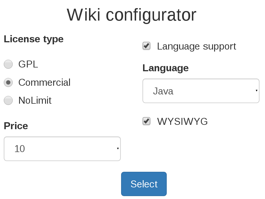
Figure 4: A possible configurator generated from the AFM of Figure 2(b)

4 Synthesis Problem

The problem tackled in this report is to synthesize an AFM (see Definition 2) from a configuration matrix (see Definition 5). Two main challenges arise: first, to preserve the configuration semantics of the input matrix; second, to produce a maximal and readable diagram.

Synthesizing an AFM that represents the exact same set of configurations (i.e. configuration semantics) as the input configuration matrix is primordial. If the AFM is too permissive, it would expose the user to illegal configurations. To prevent this situation, the algorithm must be sound (see Definition 6). Conversely, if the AFM is too constrained, it would prevent the user from selecting available configurations, resulting in unused variability. Therefore, the algorithm must also be complete (see Definition 7). Figure 5 illustrates how these two properties are related to the configuration semantics of the input configuration matrix.

Definition 6 (Soundness of AFM Synthesis).

A synthesis algorithm is sound if the resulting AFM ($afm$) represents only configurations that exist in the input configuration matrix ($cm$), i.e. $\llbracket afm\rrbracket\subseteq\llbracket cm\rrbracket$.

Definition 7 (Completeness of AFM Synthesis).

A synthesis algorithm is complete if the resulting AFM ($afm$) represents at least all the configurations of the input configuration matrix ($cm$), i.e. $\llbracket cm\rrbracket\subseteq\llbracket afm\rrbracket$.

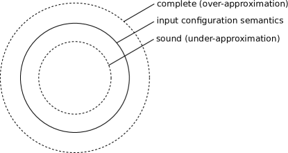
Figure 5: Soundness and completeness w.r.t the input configuration semantics

To avoid the synthesis of a trivial AFM (e.g. an AFM with the input matrix encoded in the constraint $\Phi$ and no hierarchy, i.e. $E=\emptyset$), we target a maximal AFM as output (see Definition 8). Intuitively, we enforce that the feature diagram contains as much information as possible. Definition 9 defines the AFM synthesis problem targeted in this report.

Definition 8 (Maximal Attributed Feature Model).

An AFM is maximal if its hierarchy $H$ connects every feature in $F$ and if none of the following operations are possible without modifying the configuration semantics of the AFM:

• add an edge to $E_{M}$

• add a group to $G_{MTX},G_{XOR}$ or $G_{OR}$

• move a group from $G_{MTX}$ or $G_{OR}$ to $G_{XOR}$

• add to $RC$ a non-redundant constraint that conforms to the restrictions specified in the domain knowledge.

Definition 9 (Attributed Feature Model Synthesis Problem).

Given a set of configurations sc, the problem is to synthesize an AFM $m$ such that $\llbracket sc\rrbracket=\llbracket m\rrbracket$ (i.e. the synthesis is sound and complete) and $m$ is maximal.

4.1 Equivalence of Attributed Feature Models

In Definition 9, we enforce the AFM to be maximal to avoid trivial solutions to the synthesis problem. Despite this restriction, the solution to the problem may not be unique (see Definition 10). Given a set of configurations (i.e. a configuration matrix), multiple maximal AFMs can be synthesized.

Definition 10 (Equivalence of Attributed Feature Models).

Two AFMs ($afm_{1}$ and $afm_{2}$) are equivalent if $\llbracket afm_{1}\rrbracket=\llbracket afm_{2}\rrbracket$ and if their feature diagrams (see Definition 1) are equal (i.e. only $\Phi$ can vary between the two AFMs).

This property has already been observed for the synthesis of boolean FMs [47, 41, 3, 48]. Several hierarchies of features can exist for the same configuration semantics. Extending boolean FMs with attributes exacerbates the situation. In some cases, the place of the attributes and the constraints over them can be modified without affecting the configuration semantics of the synthesized AFM.

Example. Figure 2(b) and Figure 6(a) depict two AFMs representing the same configuration matrix of Figure 2(a). They have the same configuration semantics but their attributed feature diagrams are different. In Figure 2(b), the feature WYSIWYG is placed under Wiki engine while in Figure 6(a), it is placed under the feature LicenseType. The attribute LicensePrice is placed in feature LicenseType in Figure 2(b), while it is placed in feature Wiki engine for the AFM in Figure 6(a).

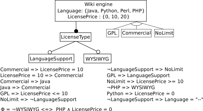
(a) Another attributed feature model representing the configuration matrix in Figure 2(a)

Information	Value
Features	WYSIWYG, LanguageSupport, LicenseType, GPL, Commercial, NoLimit
Interpretation of cells	"Yes" = presence of a feature, "No" = absence of a feature
Root	Wiki engine
Hierarchy (child $\rightarrow$ parent)	LanguageSupport $\rightarrow$ LicenseType, LicenseType $\rightarrow$ Wiki engine, WYSIWYG $\rightarrow$ LicenseType, GPL $\rightarrow$ Wiki engine, Commercial $\rightarrow$ Wiki engine, NoLimit $\rightarrow$ Wiki engine
Attributes	Language, LicensePrice
Domains	"–" is the null value of Language
Place of attributes	$\alpha(\emph{Language})=\emph{Wiki engine}$, $\alpha(\emph{LicensePrice})=\emph{Wiki engine}$
Feature groups	$\{$GPL, Commercial, NoLimit$\}$
Interesting values for RC	(LicensePrice, 10)

(b) Domain knowledge for synthesizing Figure 6(a) from Figure 2(a).

Figure 6: Another possible attributed feature model for the motivating example.

4.2 Synthesis Parametrization

As shown previously, several AFMs with the same configuration semantics can be synthesized from a single matrix. To synthesize a unique AFM (see Definition 10), our algorithm must take decisions. These decisions are based on what we call the domain knowledge which can come from heuristics, ontologies or a user of our algorithm. This domain knowledge can be provided interactively during the synthesis or as input before the synthesis. By providing this knowledge, we parametrize the algorithm to obtain a unique AFM.

The domain knowledge can be represented as a set of functions that perform the following operations:

• decide if a column should be represented as a feature or an attribute

• give the interpretation of the cells (type of the data, partial order)

• select a possible hierarchy

• select a place for each attribute among their legal positions

• select a feature group among the overlapping ones.

• provide interesting bounds for each attribute in order to compute meaningful constraints for $RC$

Examples of the information contained in domain knowledge can be found in Figures 2(c) and 6(b).

4.3 Over-approximation of the Attributed Feature Diagram

A crucial property of the output AFM of the synthesis problem is to have the exact same configuration semantics as the input configuration matrix (see Definition 9). As shown in Section 3.1, the attributed feature diagram may over-approximate the configuration semantics, i.e., $\llbracket cm\rrbracket\subseteq\llbracket FD\rrbracket$. Therefore the additional constraint $\Phi$ of an AFM (see Definition 2) is required for providing an accurate representation for any arbitrary configuration matrix.

A basic strategy for computing $\Phi$ is to directly encode the configuration matrix as a constraint, i.e., $\llbracket cm\rrbracket=\ \llbracket\Phi\rrbracket$ (see Equation 1). An advantage is that the computation is immediate and $\Phi$ is, by construction, sound and complete w.r.t. the configuration semantics. The disadvantage is that some constraints in $\Phi$ are likely to be redundant with the attributed feature diagram.

$$\Phi=\bigvee_{i=1}^{M}{\bigwedge_{j=1}^{N}{(V_{j}=c_{ij})}}\text{ with N the number of columns and M the number of rows.}$$ (1)

Ideally, $\Phi$ should express the exact and sufficient set of constraints not expressed in the attributed feature diagram, i.e., $\llbracket\Phi\rrbracket=\llbracket cm\rrbracket\setminus\llbracket FD\rrbracket$. Synthesizing a minimal set of constraint may require complex and time-consuming computations. We consider that (1) the development of efficient techniques for simplifying $\Phi$ and (2) the investigation of the usefulness and readability of arbitrary constraints are both out of the scope of this report.

Example. The AFM in Figure 2(b) exactly represents the configuration matrix of Figure 2(a). To match the configuration semantics of the configuration matrix, the AFM relies on a constraint $\Phi$. This particular constraint cannot be expressed by an attributed feature diagram as defined in Definition 1. Therefore, if $\Phi$ is not computed the AFM would represent an over-approximation of the configuration matrix. In particular, the 2 additional configurations of Table 1 would also be legal for the AFM.

This illustrates a trade-off between the expressiveness of the AFD – especially the expressiveness of $RC$ – and its over-approximation w.r.t the configuration matrix. Quantifying the difference between the two configuration semantics would be an important metric for evaluating the expressiveness of the AFD. We leave it as future work.

LicenseType	LicensePrice	LanguageSupport	Language	WYSIWYG
GPL	0	Yes	PHP	Yes
GPL	10	Yes	PHP	No

Table 1: An example of the over-approximation of the AFM in Figure 2(b) if $\Phi$ is ignored

5 Synthesis Algorithm

The input of our algorithm is a configuration matrix and some domain knowledge. It returns a maximal AFM. The domain knowledge parametrizes the synthesis in order to synthesize a unique AFM. The synthesis is divided into two parts. First, we synthesize the AFD, then we compute an additional constraint $\Phi$ to ensure the soundess of our algorithm. In this section, we focus only on the first part. A high-level description of the algorithm for synthesizing an AFD is presented in Algorithm 1. For the second part, we use Equation 1 to compute $\Phi$. (As previously stated in Section 4.3, the simplification of $\Phi$ w.r.t. diagram is out of scope of this report.)

Algorithm 1 Attributed Feature Diagram Synthesis

0   A configuration matrix $\mathbf{MTX}$ and domain knowledge $\mathbf{DK}$

0   An attributed feature diagram $\mathbf{AFM}$
Extract the features, the attributes and their domains

1   $(F,A,D,\delta)\leftarrow$ extractFeaturesAndAttributes($MTX,DK$)

Compute binary implications

2   $BI\leftarrow$ computeBinaryImplications($MTX$)

Define the hierarchy

3   $(BIG,MTXG)\leftarrow$ computeBIGAndMutexGraph($F,BI$)

4   $H\leftarrow$ extractHierarchy($BIG,DK$)

5   $\alpha\leftarrow$ placeAttributes($BI,F,A,DK$)

Compute the variability information

6   $E_{M}\leftarrow$ computeMandatoryFeatures($H,BIG$)

7   $FG\leftarrow$ computeFeatureGroups($H,BIG,MTXG,DK$)

Compute cross tree constraints

8   $RC\leftarrow$ computeConstraints($BI,DK,H,E_{M},FG$)

Create the attributed feature diagram

9   return  $AFD(F$, $H$, $E_{M}$, $FG$, $A$, $D$, $\delta$, $\alpha$, $RC)$

5.1 Extracting Features and Attributes

The first step of the synthesis algorithm is to extract the features ($F$), the attributes ($A$) and their domains ($D,\delta$). This step essentially relies on the domain knowledge to decide how each column of the matrix must be represented as a feature or an attribute. For each feature, the domain knowledge specifies which values in the corresponding column indicate the presence of the feature, and which values map to the absence of the feature. For each attribute, all the disctinct values of its corresponding column form the first part of its domain ($V_{d}$). The other parts, the null value $0_{d}$, and the partial order $<_{d}$, are computed according to the domain knowledge. At the end, we discard all the dead features, i.e. features that are always absent.

Example. Let’s consider the variable LanguageSupport in the configuration matrix of Figure 2(a). Its domain has only 2 possible values: Yes and No. According to our knowledge about Wiki engines, these values represents boolean values. Therefore, the variable LanguageSupport is identified as a feature. Following the same process, WYSIWYG and LicenseType are also identified as a feature and the other variables are identified as attributes.

5.2 Extracting Binary Implications

An important step of the synthesis is to extract binary implications between features and attributes. To compute all possible implications, we rely on the formal definition of the input configuration matrix (see Definition 5). We recall that a configuration matrix is a $M\times N$ matrix $\mathbf{C}$. Each variable $V_{j}$ of the matrix takes its value from a domain $D_{j}\in D$ defined by equation 2.

$$D_{j}=\{c_{i,j}|1\leq i\leq M\}$$ (2)

Intuitively, the domain of variable $V_{j}$ is the set of all values that appear in the $j$th column of matrix $\mathbf{C}$.

Example. Figure 2(a) shows a configuration matrix containing 5 variables and 8 configurations. The first configuration, named Confluence is $\{$Commercial, 10, Yes, Java, Yes$\}$. The domain of the variable LicensePrice is $\{0,10,20\}$.

A binary implication $B_{i,j,u,S}$ is a predicate, defined by equation 3, that maps $N$-tuples (e.g., rows of the matrix) to truth values (i.e., true and false). In binary implication $B_{i,j,u,S}$, $i$ and $j$ are integer values in $[1..N]$, $u$ belongs to $D_{i}$, and $S$ is a subset of $D_{j}$.

$$B_{i,j,u,S}(a_{1},...,a_{N})=(a_{i}=u\Rightarrow(a_{j}\in S))$$ (3)

We use $BI(\mathbf{C})$ to denote the set of all binary implications that are valid for a configuration matrix $\mathbf{C}$.

$$BI(\mathbf{C}) =\{B_{i,j,u,S}(a_{1},...,a_{N})=(a_{i}=u\Rightarrow(a_{j}\in S))|$$

$$\qquad 1\leq i,j\leq N,i\neq j,u\in D_{i},S\subseteq D_{j},$$

$$\qquad\forall 1\leq k\leq M.~{}B_{i,j,u,S}(\mathbf{c}_{k})=true\}$$

Given a configuration matrix $\mathbf{C}$, Algorithm 2 computes the set of all binary implications. First the algorithm initializes the set of binary implications $BI$ with an empty set. Then, it iterates over all pairs $(i,j)$ of columns and all configurations $c_{k}$ in $\mathbf{C}$. The objective of the inner loop is to compute the set $S(i,j,c_{k,i})$, which contains the values of those cells in column $j$ for which the corresponding cell in column $i$ is equal to $c_{k,i}$.

Algorithm 2 computeBinaryImplications

0   A configuration matrix $\mathbf{C}$

0   A set of binary implications $BI$

1   $BI\leftarrow\emptyset$

2   for all $(i,j)$ such that $1\leq i,j\leq N$ and $i\neq j$ do

3      for all $c_{k}$ such that $1\leq k\leq M$ do

4         if $S(i,j,c_{k,i})$ does not exists then

5            $S(i,j,c_{k,i})\leftarrow\{c_{k,j}\}$

6            $BI\leftarrow BI\cup\{\langle i,j,u,S(i,j,c_{k,i})\rangle\}$

7         else

8            $S(i,j,c_{k,i})\leftarrow S(i,j,c_{k,i})\cup\{c_{k,j}\}$

9   return  $BI$

In line 4, the algorithm tests if $S(i,j,c_{k,i})$ already exists, i.e. if $c_{k,i}$ is encountered for the first time. If this is the case, $S(i,j,c_{k,i})$ is initialized with the value of column $j$ for the current configuration $c_{k}$. Then, a new binary implication is created and added to the set $BI$. If $S(i,j,c_{k,j})$ already exists, the algorithm simply adds the value of column $j$ for the current configuration $c_{k}$ to the set $S(i,j,c_{k,i})$. At the end of the inner loop, $BI$ contains all the binary implications of the pair of columns $(i,j)$.

5.3 Defining the Hierarchy

The hierarchy $H$ of an AFD is similar to the hierarchy of a boolean feature model. It is a rooted tree of features such that $\forall(f_{1},f_{2})\in E,f_{1}\Rightarrow f_{2}$, i.e. each feature implies its parent. As a result, the candidate hierarchies, whose parent-child relationships violate this property can be eliminated upfront.

Example. In Figure 2(b), the feature GPL implies its parent feature LicenseType. However, GPL could not be a child of Commercial as they are mutually exclusive in the configuration matrix of Figure 2(a).

To define the hierarchy of the AFD, we rely on the Binary Implication Graph (BIG) of a configuration matrix (see Definition 11) to guide the selection of legal hierarchies. The BIG represents every implication between two features of a formula, thus representing every possible parent-child relationships a legal hierarchy can have. Therefore, we can promote a rooted tree inside the BIG as the hierarchy of the AFD. This step is performed according to the domain knowledge.

To compute the BIG, we simply iterate over the binary implications ($BI$) computed previously. For each constraint in $BI$ that represents an implication between two features, we add an edge in the BIG. As we iterate over $BI$, we take the opportunity to compute the mutex graph (see Definition 12) which will be used in the computation of feature groups.

Definition 11 (Binary Implication Graph (BIG)).

A binary implication graph of a configuration matrix $\mathbf{C}$ is a directed graph $(V_{BIG},E_{BIG})$ where $V_{BIG}=F$ and $E_{BIG}=\{(f_{i},f_{j})\mid`f_{i}\Rightarrow f_{j}^{\prime}\in BI(\mathbf{C})\}$.

After choosing the hierarchy of features, we focus on the place of the attributes. An attribute $a$ can be placed in a feature $f$ if $\neg f\Rightarrow(a=0_{a})$. As a result, the candidate features which verify this property are considered as legal positions for the attribute. To compute legal positions, we iterate over the binary implications ($BI$) to check the previous property for each attribute. Here again, we promote, according to the domain knowledge, one of the legal positions of each attribute.

Example. In Figure 2(a), the attribute Language has a domain d with "–" as its null value, i.e. $0_{d}=\text{"--"}$. This null value restricts the place of the attribute. As defined in Definition 1, an attribute can be placed in a feature if the attribute takes its null value when the feature is not selected. This property holds for the attribute Language and the feature LanguageSupport. However, the configuration MediaWiki forbids the attribute to be placed in feature WYSIWYG. The value of Language is not equal to its null value while WYSIWYG is not selected.

5.4 Computing the Variability Information

As the hierarchy of an AFD is made of features only, attributes do not impact the computation of the variability information (optional/mandatory features and feature groups). Therefore, we can rely on algorithms that can be applied on boolean FMs.

First, let’s focus on the computation of mandatory features. In an AFD, mandatory features are implied by their parents. To check this property we rely on the BIG as it represents every possible implication between two features. For each edge $(c,p)$ in the hierarchy, we check that the inverted edge $(p,c)$ exists in the BIG. If this is the case, we add this edge to $E_{M}$.

For computing feature groups, we reuse algorithms from the synthesis of boolean FMs. In the following, we briefly describe the computation of each type of group. Further details can be found in [45, 47].

For mutex-groups ($G_{MTX}$), we compute a mutex graph (see Definition 12) that contains an edge whenever two features are mutually exclusive. As a result, the mutex-groups are the maximum cliques of this mutex graph. The computation of the mutex graph is performed during the computation of the BIG by iterating over the binary constraints ($BI$).

Definition 12 (Mutex Graph).

A mutex graph of a configuration matrix $\mathbf{C}$ is an undirected graph $(V_{MTX},E_{MTX})$ where $V_{MTX}=F$ and $E_{MTX}=\{(f_{i},f_{j})\mid`f_{i}\Rightarrow\neg f_{j}^{\prime}\in BI(\mathbf{C})\}$.

For or-groups ($G_{OR}$), we translate the input matrix to a binary integer programming problem. Finding all solutions to this problem results in the list of or-groups.

For xor-groups ($G_{XOR}$), we simply list the groups that are both mutex and or-groups. However, the computation of or-groups might be time consuming as we will see in Sections 6 and 7. If this computation is disabled, we offer an alternative technique for computing xor-groups. The alternative technique consists in checking, for each mutex-group, that its parent implies the disjunction of the features of the group. For that, we iterate over the binary implications ($BI$) until we find that the property is inconsistent.

To ensure the maximality of the resulting AFM, we discard any mutex or or-groups that is also an xor-group.

Finally, the features that are not involved in a mandatory relation or a feature group are considered optional.

5.5 Computing Cross Tree Constraints

The final step of the AFD synthesis algorithm is to compute cross tree constraints ($RC$) in order to further restrict the configuration semantics of the AFD. We generate 3 kinds of constraints: requires, excludes and complex constraints.

A requires constraint represents an implication between two features. All the implications contained in the BIG (i.e. edges) that are not represented in the hierarchy or mandatory features, are promoted as requires constraints.

Example. In Figure 2(b), the implication Commercial $\Rightarrow$ Java is not represented in the hierarchy nor in mandatory features. As a consequence, this constraint is added to $RC$ and appears below the hierarchy of the FM.

Excludes constraints represent the mutual exclusion of two features. Such constraints are contained in the mutex graph. As the previously computed mutex-groups may not represent all the edges of the mutex graph, we promote the remaining edges of the mutex graph as excludes constraints.

Example. In Figure 2(b), the features NoLimit and LanguageSupport are mutually exclusive but they are not part of a mutex group. Therefore, the excludes constraint NoLimit $\Rightarrow\neg$LanguageSupport is added to $RC$ in order to represent this relation.

Finally, complex constraints are all the constraints following the grammar described in Figure 1 and involving attributes. First, we transform each constraint refering to one feature and one attribute to a constraint that respects the grammar of $RC$. Then, we focus on constraints in $BI$ that involve two attributes and we merge them according to the domain knowledge.

The domain knowledge provides the information required for merging binary implications as $(a_{i},k)$ pairs, where $a_{i}$ is an attribute, and $k$ belongs to $D_{i}$. Using the pair $(a_{i},k)$, we partition the set of all binary implications with $a_{i}=u$ on the left hand side of the implication into three categories: those with $u<k$, those with $u=k$, and those with $u>k$. Let $b_{j,1},b_{j,2},...,b_{j,p}$ be all such binary implications, belonging to the same category, and involving $a_{j}$ (i.e., each $b_{j,r}$ is of the form $(a_{i}=u_{r}\Rightarrow a_{j}\in S_{r})$). We merge these binary implications into a single one: $(a_{i}\in\{u_{1},u_{2},...,u_{p}\}\Rightarrow a_{j}\in S_{1}\cup S_{2}\cup...\cup S_{p})$. Finally, if the merged constraints can be expressed with the grammar of $RC$, we add them to $RC$. Otherwise, we discard them.

Example. From the configuration matrix of Figure 2(a), we can extract the following binary implication: $\emph{GPL}\Rightarrow\emph{LicensePrice}\in\{0,10\}$. We also note that the domain of LicensePrice is $\{0,10,20\}$. Therefore, the right side of the binary implication can be rewriten as LicensePrice $<=10$. As this constraint can be expressed by the grammar of $RC$, we add GPL $\Rightarrow$ LicensePrice $<=10$ to $RC$ as shown in Figure 2(b).

6 Theoretical Evaluation

Our algorithm presented in Section 5 addresses the synthesis problem defined in Definition 9. This definition states that the synthesized AFM must be maximal and have the same configuration semantics as the input configuration matrix. In the following, we check these two properties. We also evaluate the scalability of our algorithm by analyzing its theoretical time complexity.

6.1 Soundness and Completeness

Synthesizing an AFM that represents the exact same set of configurations (i.e. configuration semantics) as the input configuration matrix is primordial. In order to ensure this property, the synthesis algorithm must be sound (see Definition 6) and complete (see Definition 7).

6.1.1 Valid and Comprehensive Computation of Binary Implications

An AFM can be seen as the representation of a set of configurations (see Defintion 3) but also as a set of constraints over the features and attributes. These two views are equivalent but present two opposite reasonings. The former view focuses on adding configurations while the latter focuses on removing configurations. In the following, we will switch from one view to the other in order to prove the soundness and completeness of our algorithm.

A central operation in our algorithm is the computation of all the binary implications that are present in the input configuration matrix. The soundness and completeness of our algorithm are tied to a valid and comprehensive computation of these constraints. Definition 13 and Definition 14 define these two properties for the computation of binary implications, respectively.

Definition 13 (Validity of binary implications).

Let $\mathbf{C}$ be an $M\times N$ configuration matrix. A set of binary implications $BI$ is valid w.r.t. $\mathbf{C}$, iff for each $\langle i,j,u,S\rangle\in BI$ the following condition holds:

$$\forall k\in[1..M].~{}(c_{k,i}=u)\Rightarrow c_{k,j}\in S$$ (4)

Definition 14 (Comprehensiveness of binary implications).

Let $\mathbf{C}$ be an $M\times N$ configuration matrix. A set of binary implications $BI$ is comprehensive w.r.t. $\mathbf{C}$, iff:

$$\forall i,j\in[1..N],~{}\forall u\in D_{i}.~{}\exists~{}\langle i,j,u,S\rangle\in BI~{}\textnormal{such that}~{}S\subseteq D_{j}:$$ (5)

Intuitively, for each possible combination of $i,j,$ and $u$, at least one binary implication exists in $BI$.

Let $\mathbf{C}$ be an $M\times N$ configuration matrix. The set of binary implications $BI$ computed using Algorithm 2 is valid and comprehensive with respect to $\mathbf{C}$. The proof of these two properties is as follows:

Validity: Let $\langle i,j,u,S\rangle$ be an arbitrary binary implication in $BI$. In line 5 and 8 of the algorithm, we add the value of column $j$ for configuration $c_{k}$ (noted as $c_{k,j}$) to $S(i,j,c_{k,i})$. This particular $S$ is bound to $i$, $j$ and the value of the column $i$ for the configuration $c_{k}$ (noted as $c_{k,i}$). As a result, for each $k\in[1..M]$ such that $c_{k,i}=u$, $c_{k,j}$ is in $S$, and Equation 4 holds for $\langle i,j,u,S\rangle$.

Comprehensiveness: The for statements in lines 2 and 3 iterate over all values of $i$, $j$ and $u$, and generate all distinct combinations $(i,j,u)$. For each of these combinations, line 4 ensures that one binary implication is added to $BI$. Let $\langle i,j,u,S\rangle$ be a binary implication in $BI$. In addition, line 5 and 8 guarantee that the value added to $S$ is in $D_{j}$ and thus $S\subseteq D_{j}$. Therefore, Equation 5 holds for $BI$.

6.1.2 Proof of Soundness of the Synthesis Algorithm

According to Definition 6, the algorithm detailed in Section 5 is sound if all the configurations represented by the AFM exist also in the configuration matrix. To prove this property, it is equivalent to show that the constraints represented by the configuration matrix are included in the constraints represented by the AFM.

In general, the attributed feature diagram (see Definition 1) is not expressive enough to represent the constraints of the configuration matrix (see Section 4.3). To keep the algorithm sound, we rely on the additional constraint $\Phi$ of the AFM. A simple strategy is to use Equation 1 to specify the whole configuration matrix as a constraint, and include it in the AFM as $\Phi$. Such a constraint would, by construction, restrict the configuration semantics of the AFM to a subset of the configuration semantics of the matrix. Therefore, our algorithm is sound if $\Phi$ is carefully defined. Otherwise, it may represent an overapproximation of the input configuration matrix (see Section 4.3).

6.1.3 Proof of Completeness of the Synthesis Algorithm

To prove the completeness of our algorithm, we have to show that all the configurations represented by the configuration matrix exist also in the synthesized AFM (see Definition 7). It is equivalent to show that all the constraints represented by the AFM are included in the constraints represented by the configuration matrix. A first observation is that, apart from or-groups, xor-groups and $\Phi$, the AFM is constructed from a set of binary implications computed by Algorithm 2 (step 2 of Algorithm 1).

As proved in Section 6.1.1, the computed binary implications are valid. Therefore, all the constraints presented by these implications are included in the configuration matrix. All the subsequent computations relying on the binary implications do not introduce new constraints. They only reuse and transform these binary implications into feature modeling concepts.

For or-groups and xor-groups, we reuse existing techniques that rely on the input configuration matrix. These techniques are designed for a similar context of FM synthesis and ensure the completeness of the resulting FM [45, 47]. In our context of AFMs, the features and the attributes are separated in two distinct sets, repesctively $F$ and $A$. Moreover, the attributes do not enter in the definition of the hierarchy $H$ or the feature groups. As a consequence, the adaptation of techniques for computing or-groups and xor-groups to the context of AFMs is straightforward and guarantees the completeness.

Finally, $\Phi$ as computed by Equation 1 is equivalent to the configuration matrix. Therefore, adding such a $\Phi$ to AFM does not exclude from it any of the configurations represented by the configuration matrix.

Overall, each step of the algorithm of Section 5 guarantees the property of completeness. Therefore, the whole synthesis process ensures completeness.

6.2 Maximality

Another challenge is to ensure the maximality of the synthesized AFM in order to avoid trivial answers to the AFM synthesis problem (see Section 5). In this section, we prove that Algorithm 1 produces a maximal attributed feature model. This is stated in Theorem 1.

Theorem 1 (Maximality of the configuration semantics).

Let $M$ be a configuration matrix, and $AFM$ be a sound and complete synthesis of $M$, generated using Algorithm 1. Then, $AFM$ is also maximal.

Proof.

To prove the maximality of $AFM=\langle F,H,E_{M},G_{MTX},G_{XOR},G_{OR},A,D,\delta\alpha,RC\rangle$, we show that all conditions in Definition 8 hold for $AFM$:

$H$ connects every feature in $F$. The algorithm ensures that the synthesized hierarchy contains all the features of the configuration matrix. The hierarchy is a rooted tree which is extracted from the binary implication graph (BIG) in step 4 of Algorithm 1. By construction (see Definition 11), the BIG contains all the features. Moreover, the comprehensive computation of the binary implications (see Section 6.1.1) ensures that the BIG represents all possible implications of the configuration matrix. We can define a hierarchy of an AFM as a spanning tree of the BIG. Therefore, every spanning tree of the BIG is a possible hierarchy for the AFM and every possible hierarchy is a spanning tree of the BIG [48]. The existence of a single spanning tree is not generally ensured for a binary implication graph computed from any arbitrary configuration matrix. Specifically, the BIG may contain more than a single connected component. In such cases, we simply create a new root feature $r$ in the BIG, and connect every feature in $F$ to $r$. As a consequence, line 3 of the algorithm always generates a connected graph. The extractHierarchy routine in line 4 of Algorithm 1, uses the domain knowledge to chose one spanning tree of the BIG as $H$. Therefore, $H$ is guaranteed to be a tree containing all features in $F$.

Adding an edge to $E_{m}$ changes the configuration semantics of $AFM$ ($\llbracket AFM\rrbracket$). The algorithm ensures that no edge can be added to the set of mandatory edges, $E_{m}$, without changing the configuration semantics of the AFM (i.e., adding or removing items from $\llbracket AFM\rrbracket$). $E_{m}$ represents every edge $(f_{1},f_{2})$ of the hierarchy $H$ such that $f_{1}\Leftrightarrow f_{2}$. In line 6 of the algorithm, for each edge $(f_{1},f_{2})$ in the hierarchy $H$, we add an edge $(f_{2},f_{1})$ to $E_{m}$, iff $(f_{2},f_{1})$ exists in the BIG. As mentioned previously, the BIG exactly represents all possible implications of the configuration matrix. Adding any other edge to $E_{m}$ implies that the added edge does not exist in BIG. Therefore, no edge can be further added to $E_{m}$ without changing the configuration matrix, which corresponds to the configuration semantics of the AFM.

Adding an item to any of $G_{MTX}$, $G_{OR}$, or $G_{XOR}$ changes $\llbracket AFM\rrbracket$. The computation of feature groups is entirely performed with existing techniques that are designed for the synthesis of boolean FMs. Our definition of a maximal AFM (see Definition 1 and 8) preserves the definition of feature groups and the notion of maximality used in boolean FMs. Moreover, the attributes are clearly separated from features and are not part of the feature groups. Therefore, the techniques designed for boolean FMs are not impacted by the attributes and keep their properties (soundness, completeness and maximality). As we are using techniques that are designed for synthesizing sound, complete and maximal boolean FMs [45, 47], no group can be added to $G_{MTX}$, $G_{OR}$ $G_{XOR}$ without changing the configuration semantics of the $AFM$.

Moving any item from $G_{MTX}$ or $G_{OR}$ to $G_{XOR}$ changes $\llbracket AFM\rrbracket$. An xor-group is a feature-group that is both a mutex-group and an or-group. In Algorithm 1, we promote every mutex-group that is also an or-group as an xor-group. Moreover, the previous property of maximality ensures that all the possible feature groups are computed. Therefore, moving another group from $G_{MTX}$ or $G_{OR}$ to $G_{XOR}$ is impossible without changing the configuration semantics of the AFM.

Adding a non-redundant constraint to $RC$ changes $\llbracket AFM\rrbracket$. As shown in the grammar of $RC$ in Figure 1, all readable constraints are implications between values of features or attributes. We compute the set of all such binary implications in line 2 of the algorithm. As proven in Section 6.1.1, Algorithm 2 perform a comprehensive computation of binary implications in BI. Any additional constraint is therefore, either redundant, forbidden by the domain knowledge (i.e. its numerical literal is not part of the interesting values) or inconsistent with configuration matrix $M$. The latter implies that adding a non-redundant constraint to $RC$ would change the configuration semantics of $AFM$.

Overall, every property of the maximality is verified in the resulting AFM of our algorithm.

∎

6.3 Complexity analysis

The manual elaboration of an AFM is error-prone and time-consuming. As we showed previously, the soundness and completeness of our algorithm address the first problem. For the second problem, we have to evaluate the time complexity of our algorithm. It depends on 3 characteristics of the input configuration matrix:

• number of variables (features + attributes): $v=f+a$

• number of configurations: $c$

• maximum domain size (i.e. maximum number of distinct values for a variable): $d$

In the following, we analyze the complexity for each step of Algorithm 1 and 2.

6.3.1 Extracting Features and Attributes

The first step of Algorithm 1 is the extraction of features, attributes and their domains. This extraction simply consists in running through the configuration matrix to gather the domains and identify features and attributes. The size of the matrix is characterized by the number of variables (columns) and the number of configurations (rows). Therefore, the complexity is $O(v.c)$.

6.3.2 Extracting Binary Implications

The extraction of binary implications is computed by Algorithm 2 whose complexity is as follows. The outer for loop of lines 2-8 iterates over all pairs of variables in the configuration matrix ($O(v^{2})$). The inner for loop of lines 3-8 iterates over all configurations ($O(c)$). In this loop, we perform 2 types of operations: checking the existence of the set $S(i,j,c_{k,i})$ in line 4 and adding one element to a set. Checking the existence of $S(i,j,c_{k,i})$, for a given $i$ and $j$, involves searching for an element in a map that has potentially $d$ elements. Therefore, its complexity is $O(d)$. The latter operation is performed on a set that accesses its elements by a hash function. Adding an element to such a set has a complexity of $O(1)$. Overall, the complexity of the computation of binary implications is $O(v^{2}.c.d)$.

6.3.3 Defining the Hierarchy

In line 3, we iterate over all the binary implications to compute the binary implication graph and the mutex graph. For each binary implication, if it represents an implication between two features, we add an edge to the binary implication graph. If the binary implication represents a mutual exclusion between two features, we add an edge to the mutex graph. Both checks are done in a constant time. Therefore, the complexity of this step depends on the number of binary implications. As explained in Algorithm 2, we create a binary implication for each pair of variables $(i,j)$ and for each value $c_{k,i}$ in the domain of the $i$. It results in a maximum of $v^{2}.d$ binary implications. As a consequence, the complexity of line 3 is $O(v^{2}.d)$.

In line 4, we compute the hierarchy of the AFM by selecting a tree in the binary implication graph. This step is performed by the domain knowledge (i.e. by a user or an external algorithm). In [48], we propose an algorithm for this task which has a time complexity of $O(f.log(f^{2}))$.

In line 5, we compute all the possible places for each attribute. We recall that an attribute $a$ can be placed in the feature $f$ if $\neg f\Rightarrow(a=0_{a})$, with $0_{a}$ being the null value of the domain of $a$. We first initialize the possible places for all attributes as an empty set. Then, we iterate over each binary implication $\{\langle i,j,u,S\rangle\}$ in order to add the valid places. The loop has a complexity of $O(v^{2}.d)$ as it represents the maximum number of binary implications. A valid place is identified as follows. First, we check that $i$ is a feature, $j$ is an attribute and that $u$ represents the absence of the feature $i$. Then, we verify that $S$ is equal to the null value of the domain of $j$. If all these properties are respected, the feature $i$ is thus a valid place for the attribute $j$ and can be added to its possible places. These verifications have a complexity of $O(d$). Overall, the complexity of this step is $O(v^{2}.d^{2})$.

6.3.4 Computing the Variability Information

The computation of variability information is done in two steps: mandatory features and feature groups. For detecting mandatory features, we iterate over every edge of the hierarchy. As the hierarchy is a tree containing all the features as nodes, the number of edges is exactly equal to $f-1$. For each edge, we check that the inverted edge exists in the binary implication graph. This check is performed with a complexity of $O(f)$ in our implementation. Overall, the complexity is $O(f^{2})$.

For feature groups, we rely on existing techniques that are developed in [45, 47]. We summarize the results of the complexity analysis of these techniques.

The computation of mutex groups consists in finding maximal cliques in the mutex graph. As the mutex graph contains all the features as nodes, the complexity of this operation is $O(3^{f/3})$ [70].

For or-groups, the algorithm relies on a binary integer programming which is an NP-complete problem.

For the computation of xor-groups, there are two alternatives. The first one assumes the computation of or-groups. For each or-group, it iterates through the mutex-groups to check if there exists an equivalent group (i.e. same parent and same children). As the number of groups is bounded by the number of features, the two iterations have a complexity of $O(f^{2})$. Checking if two groups are equivalent consists in checking the equality of two sets. The maximum size for a group is also bounded by the number of features. The check is performed with a complexity of $O(f^{2})$. Overall, this first technique for computing xor-groups is $O(f^{4})$.

The second technique do not assume the computation of or-groups. It iterates over every mutex-group and checks that, for each configuration, the parent of the group implies the disjunction of the features of the group. Checking this property depends on the size of the mutex-group, which is bounded by the number of features $f$. Overall, the complexity of this second technique for computing xor-groups is $O(f^{2}.c)$

6.3.5 Computing Cross Tree Constraints

The computation of cross tree constraints ($RC$) is performed in three steps.

First, the requires constraints are extracted from the binary implication graph. The algorithm iterates over every edge of the graph and checks if it exists either in the mandatory features or in the hierarchy. The binary implication graph is composed of the features as nodes and thus contains at most $f^{2}$ edges. In addition, the number of edges represented by the mandatory features and the hierarchy is bounded by the number of features $f$. Therefore, the complexity of this step is $O(f^{3})$.

Then, the excludes constraints are extracted from the mutex graph by looking for all the edges that are in the mutex graph but not in any mutex-group. The algorithm iterates over every edge of the mutex graph and checks that it does not exist in the mutex-groups. Like the binary implication graph, the mutex graph contains at most $f^{2}$ edges. Moreover, the mutex-groups represent at most $f$ edges (size of the hierarchy). Therefore, checking if an edge exists in the mutex-groups has a complexity of $O(f)$. Overall, the complexity of this step is $O(f^{3})$.

Finally, the complex constraints are extracted from the binary implications computed in line 2 of Algorithm 1. This extraction is done in two steps. In the first step, the algorithm iterates over every binary implication, which results in a complexity of $O(v^{2}.d)$. Then, binary implications that refer to a particular pair of attributes (e.g., $(a_{i},a_{j})$) are divided into three categories based on the bound specified on the first attribute, by the domain knowledge. The items in each category are then merged. To speed up the detection of implications that need to be merged, we store the implications in a map indexed by the pairs of attributes. Therefore, the algorithm is working on three maps that have at most $v^{2}$ elements. Thus, the complexity of an operation on the map is $O(v^{2})$. Merging two binary constraints $(a_{i},u_{1},a_{j},S_{1})$ and $(a_{i},u_{2},a_{j},S_{2})$ consists in computing the union of $S_{1}$ and $S_{2}$. These sets contain values of the attribute $a_{j}$ and have a maximum size of $d$. Therefore, the complexity for merging two binary constraints is $O(d)$ and the total complexity of this first step is $O(v^{2}.d(v^{2}+d))=O(v^{4}.d+v^{2}.d^{2})$.

In the second step of the extraction of constraints, we iterate over the three maps previously computed. Each map has potentially $v^{2}$ elements. The complexity of the loop is thus $O(v^{2})$. In these maps, the value of each element ($a_{i},a_{j}$) is composed of the result of the previous merge operations, which is a set $S$ of at most $d$ elements. We check that $S$ can be represented as “$a_{j}$ OP $k$”, with OP a comparison operator from the grammar of $RC$ and $k$ a value of the domain of $a_{j}$, specifying the bound on it. If this representation is possible, we add it as a complex constraint to $RC$. In our implementation this check has a complexity of $d^{2}$. Therefore, the complexity of the second step is $O(v^{2}.d^{2})$.

Overall, the complexity of the computation of complex constraints is $O(v^{4}.d+v^{2}.d^{2})$.

6.3.6 Overall Complexity

The time complexity analysis of Algorithm 1 shows that, apart from the computation of mutex-groups and or-groups, the synthesis of an attributed feature diagram has a polynomial time complexity. In particular, its complexity is $O(v^{4}.d+v^{2}.d^{2}+v^{2}.c.d)$. The complexity of the computation of mutex-groups and or-groups are exponential and NP-complete, respectively. They represent the hardest parts of Algorithm 1 from a theoretical point of view. To obtain an AFM, we have to take into account the computation of $\Phi$. With our algorithm in Equation 1, we simply iterate over each value of the configuration matrix, which results in a complexity of $O(v.c)$.

7 Empirical Evaluation

For this practical evaluation, we evaluate the time complexity of the AFD synthesis algorithm described in Algorithm 1. In the following experiments, the algorithm takes random matrices as input. We evaluate its scalability over 3 caracteristics of the input: number of features and attributes, number of configurations and the maximum number of distinct values for an attribute.

7.1 Experimental Settings

For this evaluation, we use randomly generated matrices as input. Our random matrix generator has 3 parameters :

• number of variables (features and attributes)

• number of configurations

• maximum domain size (i.e. maximum number of distinct values in a column)

The type of each variable (feature or attribute) is randomly selected according to a uniform distribution. An important property is that our generator does not ensure that the number of configurations and the maximum domain size are reached at the end of the generation. Any duplicated configuration or missing value of a domain is not corrected. Therefore, the parameters entered for our experiments may not reflect the real properties of the generated matrices. To avoid any misinterpretation or bias, we present the concrete numbers in the following results.

Moreover, to reduce fluctuations caused by the random generator, we perform the experiments at least 100 times for each triplet of parameters. In order to get the results in a reasonable time, we used a cluster of computers. Each node in the cluster is composed of two Intel Xeon X5570 at 2.93 Ghz with 24GB of RAM.

7.2 Expected practical complexity

The analysis of the theoretical time complexity of Algorithm 1 shows two hard parts (see Section 6.3). The first hard part is the computation of mutex-groups, which has an exponential worst-case complexity. In [47], She et al. show that the algorithm for computing mutex-groups takes a few seconds for FMs with up to 290 features and can scale to FMs with 5000 features. We also note that our dataset produces mutex graphs with 6 edges in average and 93.8% of the mutex graphs contain absolutely no edges. In such cases, computing maximal cliques (i.e. computing mutex-groups) is trivial. Therefore, we expect a non significant impact of the computation of mutex-groups on the practical complexity.

The second hard part of the algorithm is the computation of or-groups, which is NP-complete. Unlike mutex groups, She et al. show that the computation of or-groups hardly scales [47]. In Section 7.3.1, we confirm this observation by evaluating the scalability of the computation of or-groups w.r.t the number of variables. Based on this observation, we deactivated the computation of or-groups in the rest of the experiments.

For the rest of the algorithm, the theoretical complexity is polynomial: $O(v^{4}.d+v^{2}.d^{2}+v^{2}.c.d)$. We note that some operations in the algorithm (e.g. the computation of complex constraints) rely on the use of data structures based on hash functions. An operation on such data structure has a linear worst case complexity. However, the probability of reaching the worst case complexity is very low in practice. Moreover, the size of the mutex graph also impacts the practical complexity of the computation of excludes constraints which has a theoretical complexity of $O(f^{3})$. The effective size of other data structures used during the algorithm may further reduce the practical complexity. Therefore, we expect a lower practical complexity than the theoretical one.

7.3 Results

We evaluate the scalability of the AFD synthesis algorithm w.r.t to the 3 parameters of our random matrix generators: number of variables, number of configurations and maximum domain size. In the following, we present the results as figures. When applicable, we include average values using red points, and linear regression trendlines using black lines. To illustrate how the linear regression fits the data, we also compute the pearson correlation coefficient.

7.3.1 Or groups

As shown in Section 6, the computation of or-groups is NP-complete and represents one of the hardest parts of the synthesis algorithm. As such, it may be time consuming and form the main performance bottleneck of the algorithm. Our first experiment evaluates the scalability of the or-groups computation w.r.t the number of features. We measure the time needed to compute the or-groups from a matrix with 1000 configurations, a maximum domain size of 10 and a number of variables ranging from 5 to 70. To keep a reasonable time for the execution of the experiment, we set a timeout at 30 minutes. Results are presented in Figure 7.

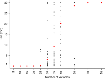
Figure 7: Scalability of or-groups computation w.r.t the number of variables

The results show that the computation of or-groups quickly becomes time consuming. The 30 minutes timeout is reached with matrices containing only 30 variables. With at least 60 variables, the timeout is systematically reached. Actually, or-groups represent a small part of the AFD. For example, only one or-group was found in the Linux feature model [31]. Dedicating so much time for such a small contribution to the feature model is not worth it. Therefore, we deactivated the computation of or-groups in the following experiments.

7.3.2 Scalability w.r.t the number of variables

To evaluate the scalability with respect to the number of variables, we perform the synthesis of random matrices with 1000 configurations, a maximum domain size of 10 and a number of variables ranging from 5 to 2000. In Figure 8, we present the square root of the time needed for the whole synthesis compared to the number of variables.

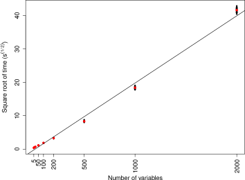
Figure 8: Scalability w.r.t the number of variables

The results indicate that the square root of the time grows linearly with the number of variables, with a correlation coefficient of 0.997. We observe a difference between pratical and theoretical complexity. As mentioned in Section 7.2, several factors can explain this lower complexity. Overall, the results of this experiment are consistent with the computed theoretical complexity.

7.3.3 Scalability w.r.t the number of configurations

To evaluate the scalability with respect to the number of configurations, we perform the synthesis of random matrices with 100 variables, a maximum domain size of 10 and a number of configurations ranging from 5 to 200,000. With 100 variables, and 10 as the maximum domain size, we can generate $10^{100}$ distinct configurations. This number is big enough to ensure that our generator can randomly generate 5 to 200,000 distinct configurations. The time needed for the synthesis is presented in Figure 9.

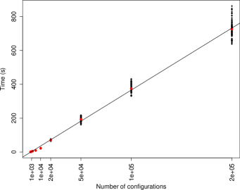
Figure 9: Scalability w.r.t the number of configurations

The results indicate that the time grows linearly with the number of configurations. Again, the correlation coefficient of 0.997 confirms that the practical time complexity is consistent with the theoretical complexity.

7.3.4 Scalability w.r.t the maximum domain size

Parameter	5	10	20	50	100	200	500	1,000	2,000	5,000	10,000
Generated	5	10	20	50	100	200	500	1,000	1,995	4,385	6,416

Table 2: Difference between the intended maximum domain size and the effective value

To evaluate the scalability wit respect to the maximum domain size, we perform the synthesis of random matrices with 10 variables, 10,000 configurations and a maximum domain size ranging from 5 to 10,000. The first row of Table 2 lists the intended values for the maximum domain size, used as input to the matrix generator. The second row of the table shows the effective maximum domain size in each case. In Figure 10, we present the square root of the time needed for the synthesis.

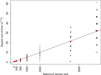
Figure 10: Scalability w.r.t the maximum domain size

As shown in the second row of Table 2, and depicted in Figure 10, maximum domain sizes 5000 and 10,000 were not reached during the experiment. This does not impact the validity of our results as we show the value of the domain size for the output of the generator and not for its parameters.

We also notice that for each value of the domain size, the points are distributed in small groups. For instance, we can see nine groups of points for a maximum domain size of 2000. Each group represents the execution of our algorithm with matrices that have the same number of attributes. However, we see that the number of attributes does not significantly affect the maximum domain size (the maximum domain size is approximately the same for all groups of results).

The results indicate that the square root of the time grows linearly with the maximum domain size. The correlation coefficient of 0.932 confirms that the practical time complexity is consistent with the theoretically computed time complexity.

7.3.5 Time Complexity Distribution

To further understand the practical time complexity of the algorithm, we analyze its distribution over different steps of the algorithm. In Figure 11, we depict the average distribution for all previous experiments that do not contain the computation of or-groups.

The results clearly show that the major part of the algorithm is spent on the computation of binary implications, which has a complexity of $O(v^{2}.c.d)$ as shown in Section 6.3.2, and complex constraints for $RC$, which has a complexity of $O(v^{4}.d+v^{2}.d^{2})$ as shown in Section 6.3.5. The rest of the synthesis represents less than 10% of the total duration. Optimizing these two main steps would significantly decrease the time necessary for synthesizing an AFM.

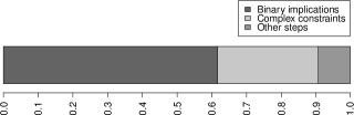
Figure 11: Time complexity distribution for all experiments without or-groups computation

8 Threats to Validity

An external threat is that our evaluation is based on the generation of random matrices. Using such matrices may not reflect the practical complexity of our algorithm with a realistic data set. We leave this kind of evaluation as future work.

Evaluating the scalability on a cluster of computers instead of a single one may impact the scalability results and is an internal threat to validity. We limited this threat to validity by using a cluster composed of identical nodes. Even if the nodes do not represent a standard computer, we only modify the absolute values of the experiments. The practical complexity of the algorithm is not influenced by this gain of processing power. Moreover, all the necessary data for the experiments are present in the local disks of the nodes thus avoiding any network related issue. Finally, we performed 100 runs for each set of parameters in order to reduce any variation of performance.

Another threat to internal validity is related to our implementation of the algorithm. To check the correctness of the implementation, we have manually reviewed some resulting AFMs. We also tested the algorithm against a set of manually designed configuration matrices. Each matrix represents a minimal example of a construct of an AFM (e.g. one of the matrices represents an AFM composed of a single xor-group). The test suite covers all the concepts in an AFM. None of these experiments revealed any anomalies in our implementation.

9 Conclusion

We presented the foundations for synthesizing attributed feature models (AFMs) from product descriptions. We introduced the formalism of configuration matrix for documenting a set of products along different Boolean and numerical values. We then sought to understand the relationship between configuration matrices and AFMs. The key contributions of the report can be summarized as follows:

• We described formal properties of AFMs and established semantic correspondences with the formalism of configuration matrices. We demonstrated why an attributed feature diagram (i.e., the diagrammatic representation of an AFM typically read and maintain by a human) may represent an overapproximation of the configuration matrix;

• We designed and implemented a comprehensive, parametrizable synthesis algorithm. We showed that the algorithm is (1) sound and complete w.r.t the configuration semantics of the input configuration matrix (2) synthesizes maximal feature diagrams;

• We theoretically and empirically evaluated the scalability of the synthesis algorithm.

Numerous kinds of artefacts and problems are amenable to configuration matrices, opening perspectives for applying the synthesis of AFMs. As future work, we plan to further study some properties of the synthesis – like scalability (performance), readability and usefulness of computed constraints, and the over-approximation effect. We are currently investigating the use of AFM synthesis in practical settings.

References

- [1] K. Czarnecki and U. Eisenecker, Generative Programming: Methods, Tools, and Applications. Addison-Wesley, 2000.
- [2] K. Czarnecki, C. H. P. Kim, and K. T. Kalleberg, “Feature models are views on ontologies,” in SPLC ’06. IEEE, 2006, pp. 41–51.
- [3] K. Czarnecki and A. Wasowski, “Feature diagrams and logics: There and back again,” in SPLC’07. IEEE, 2007, pp. 23–34.
- [4] A. Hubaux, T. T. Tun, and P. Heymans, “Separation of concerns in feature diagram languages: A systematic survey,” ACM Computing Surveys, 2013.
- [5] Q. Boucher, A. Classen, P. Faber, and P. Heymans, “Introducing TVL, a text-based feature modelling language,” in VaMoS’10, 2010, pp. 159–162.
- [6] M. Cordy, P.-Y. Schobbens, P. Heymans, and A. Legay, “Beyond boolean product-line model checking: dealing with feature attributes and multi-features,” in ICSE’13, 2013, pp. 472–481.
- [7] M. H. ter Beek, S. Gnesi, and F. Mazzanti, “VMC: A tool for the analysis of variability in software product lines,” ERCIM News, vol. 2013, no. 93, 2013. [Online]. Available: http://ercim-news.ercim.eu/en93/ri/vmc-a-tool-for-the-analysis-of-variability-in-software-product-lines
- [8] T. Thüm, S. Apel, C. Kästner, I. Schaefer, and G. Saake, “A classification and survey of analysis strategies for software product lines,” ACM Computing Surveys, 2014.
- [9] Q. Boucher, E. Abbasi, A. Hubaux, G. Perrouin, M. Acher, and P. Heymans, “Towards more reliable configurators: A re-engineering perspective,” in PLEASE’12 Int’l workshop at ICSE’12, ser. , 2012.
- [10] E. Khalil Abbasi, A. Hubaux, M. Acher, Q. Boucher, and P. Heymans, “The anatomy of a sales configurator: An empirical study of 111 cases,” in CAiSE’13, 2013.
- [11] A. Hubaux, M. Acher, T. T. Tun, P. Heymans, P. Collet, and P. Lahire, Domain Engineering: Product Lines, Conceptual Models, and Languages. Springer, 2013, ch. Separating Concerns in Feature Models: Retrospective and Multi-View Support.
- [12] J. Guo, E. Zulkoski, R. Olaechea, D. Rayside, K. Czarnecki, S. Apel, and J. M. Atlee, “Scaling exact multi-objective combinatorial optimization by parallelization,” in ASE ’14, 2014, pp. 409–420.
- [13] D. Benavides, S. Segura, and A. Ruiz-Cortes, “Automated analysis of feature models 20 years later: a literature review,” Information Systems, vol. 35, no. 6, 2010.
- [14] T. Berger, D. Nair, R. Rublack, J. M. Atlee, K. Czarnecki, and A. Wasowski, “Three cases of feature-based variability modeling in industry,” in MODELS, 2014, pp. 302–319.
- [15] S. Apel, D. Batory, C. Kästner, and G. Saake, Feature-Oriented Software Product Lines: Concepts and Implementation. Springer-Verlag, 2013.
- [16] A. Hubaux, P. Heymans, P.-Y. Schobbens, and D. Deridder, “Towards multi-view feature-based configuration,” in REFSQ’10, ser. LNCS, 2010, vol. 6182, pp. 106–112.
- [17] H. Eichelberger and K. Schmid, “A systematic analysis of textual variability modeling languages,” in 17th International Software Product Line Conference, SPLC 2013, 2013, pp. 12–21. [Online]. Available: http://doi.acm.org/10.1145/2491627.2491652
- [18] A. Classen, Q. Boucher, and P. Heymans, “A text-based approach to feature modelling: Syntax and semantics of TVL,” Sci. Comput. Program., vol. 76, no. 12, pp. 1130–1143, 2011.
- [19] K. Bak, K. Czarnecki, and A. Wasowski, “Feature and meta-models in clafer: mixed, specialized, and coupled,” in SLE’10, ser. LNCS. Springer, 2011, pp. 102–122.
- [20] C. Seidl, I. Schaefer, and U. Aßmann, “Capturing variability in space and time with hyper feature models,” in VaMoS. ACM, 2014, p. 6.
- [21] N. Siegmund, M. Rosenmüller, M. Kuhlemann, C. Kästner, S. Apel, and G. Saake, “Spl conqueror: Toward optimization of non-functional properties in software product lines,” Software Quality Control, vol. 20, no. 3-4, pp. 487–517, Sep. 2012.
- [22] N. Siegmund, S. S. Kolesnikov, C. Kästner, S. Apel, D. S. Batory, M. Rosenmüller, and G. Saake, “Predicting performance via automated feature-interaction detection,” in ICSE, M. Glinz, G. C. Murphy, and M. Pezzè, Eds. IEEE, 2012, pp. 167–177.
- [23] N. Siegmund, M. RosenmüLler, C. KäStner, P. G. Giarrusso, S. Apel, and S. S. Kolesnikov, “Scalable prediction of non-functional properties in software product lines: Footprint and memory consumption,” Inf. Softw. Technol., vol. 55, no. 3, pp. 491–507, Mar. 2013.
- [24] J. Guo, K. Czarnecki, S. Apel, N. Siegmund, and A. Wasowski, “Variability-aware performance prediction: A statistical learning approach,” in ASE, E. Denney, T. Bultan, and A. Zeller, Eds. IEEE, 2013, pp. 301–311.
- [25] S. S. Kolesnikov, S. Apel, N. Siegmund, S. Sobernig, C. Kästner, and S. Senkaya, “Predicting quality attributes of software product lines using software and network measures and sampling,” in VaMoS, S. Gnesi, P. Collet, and K. Schmid, Eds. ACM, 2013, p. 6.
- [26] Guo, Jianmei and Edward Zulkoski and Rafael Olaechea and Derek Rayside and Krzysztof Czarnecki and Apel, Sven and Atlee, Joanne M., “Scaling exact multi-objective combinatorial optimization by parallelization,” in ASE. ACM, 2014.
- [27] M. Alférez, J. A. Galindo, M. Acher, and B. Baudry, “Modeling variability in the video domain: Language and experience report,” INRIA, Rapport de Recherche RR-8576, jul 2014. [Online]. Available: http://hal.inria.fr/hal-01023159
- [28] J.-M. Davril, E. Delfosse, N. Hariri, M. Acher, J. Cleland-Huang, and P. Heymans, “Feature model extraction from large collections of informal product descriptions,” in ESEC/FSE’13, 2013.
- [29] M. Acher, A. Cleve, G. Perrouin, P. Heymans, C. Vanbeneden, P. Collet, and P. Lahire, “On extracting feature models from product descriptions,” in VaMoS’12. ACM, 2012, pp. 45–54.
- [30] M. Acher, A. Cleve, P. Collet, P. Merle, L. Duchien, and P. Lahire, “Extraction and evolution of architectural variability models in plugin-based systems,” Software and Systems Modeling (SoSyM), 2013.
- [31] S. She, R. Lotufo, T. Berger, A. Wasowski, and K. Czarnecki, “Reverse engineering feature models,” in ICSE’11. ACM, 2011, pp. 461–470.
- [32] U. Ryssel, J. Ploennigs, and K. Kabitzsch, “Extraction of feature models from formal contexts,” in FOSD’11, 2011, pp. 1–8.
- [33] E. Bagheri, F. Ensan, and D. Gasevic, “Decision support for the software product line domain engineering lifecycle,” Automated Software Engineering, vol. 19, no. 3, pp. 335–377, 2012.
- [34] A. Ferrari, G. O. Spagnolo, and F. dell’Orletta, “Mining commonalities and variabilities from natural language documents,” in SPLC, T. Kishi, S. Jarzabek, and S. Gnesi, Eds. ACM, 2013, pp. 116–120.
- [35] V. Alves, C. Schwanninger, L. Barbosa, A. Rashid, P. Sawyer, P. Rayson, C. Pohl, and A. Rummler, “An exploratory study of information retrieval techniques in domain analysis,” in SPLC’08. IEEE, 2008, pp. 67–76.
- [36] N. Niu and S. M. Easterbrook, “Concept analysis for product line requirements,” in AOSD’09, K. J. Sullivan, A. Moreira, C. Schwanninger, and J. Gray, Eds. ACM, 2009, pp. 137–148.
- [37] N. Weston, R. Chitchyan, and A. Rashid, “A framework for constructing semantically composable feature models from natural language requirements,” in SPLC’09. ACM, 2009, pp. 211–220.
- [38] K. Chen, W. Zhang, H. Zhao, and H. Mei, “An approach to constructing feature models based on requirements clustering,” in RE’05, 2005, pp. 31–40.
- [39] S. Nadi, T. Berger, C. Kästner, and K. Czarnecki, “Mining configuration constraints: Static analyses and empirical results,” in Proceedings of the 36th International Conference on Software Engineering (ICSE), 6 2014.
- [40] M. Janota, V. Kuzina, and A. Wasowski, “Model construction with external constraints: An interactive journey from semantics to syntax,” in MODELS’08, ser. LNCS, vol. 5301, 2008, pp. 431–445.
- [41] M. Acher, P. Heymans, A. Cleve, J.-L. Hainaut, and B. Baudry, “Support for reverse engineering and maintaining feature models,” in VaMoS’13. ACM, 2013.
- [42] E. N. Haslinger, R. E. Lopez-Herrejon, and A. Egyed, “Reverse engineering feature models from programs’ feature sets,” in WCRE’11. IEEE, 2011, pp. 308–312.
- [43] R. E. Lopez-Herrejon, J. A. Galindo, D. Benavides, S. Segura, and A. Egyed, “Reverse engineering feature models with evolutionary algorithms: An exploratory study,” in SSBSE’12, ser. LNCS, vol. 7515. Springer, 2012, pp. 168–182.
- [44] E. N. Haslinger, R. E. Lopez-Herrejon, and A. Egyed, “On extracting feature models from sets of valid feature combinations,” in FASE’13, ser. LNCS, vol. 7793, 2013, pp. 53–67.
- [45] N. Andersen, K. Czarnecki, S. She, and A. Wasowski, “Efficient synthesis of feature models,” in Proceedings of SPLC’12. ACM, 2012, pp. 97–106.
- [46] K. Czarnecki, S. She, and A. Wasowski, “Sample spaces and feature models: There and back again,” in SPLC’08, 2008, pp. 22–31.
- [47] S. She, U. Ryssel, N. Andersen, A. Wasowski, and K. Czarnecki, “Efficient synthesis of feature models,” Information and Software Technology, vol. 56, no. 9, pp. 1122–1143, 2014.
- [48] G. Bécan, M. Acher, B. Baudry, and S. Ben Nasr, “Breathing ontological knowledge into feature model synthesis: an empirical study,” Empirical Software Engineering, 2015.
- [49] R. E. Lopez-Herrejon, L. Linsbauer, J. A. Galindo, J. A. Parejo, D. Benavides, S. Segura, and A. Egyed, “An assessment of search-based techniques for reverse engineering feature models,” Journal of Systems and Software, 2014.
- [50] G. Bécan, S. B. Nasr, M. Acher, and B. Baudry, “WebFML: Synthesizing Feature Models Everywhere,” in SPLC’14, 2014.
- [51] N. Hariri, C. Castro-Herrera, M. Mirakhorli, J. Cleland-Huang, and B. Mobasher, “Supporting domain analysis through mining and recommending features from online product listings,” IEEE Transactions on Software Engineering, vol. 99, no. PrePrints, p. 1, 2013.
- [52] L. Yi, W. Zhang, H. Zhao, Z. Jin, and H. Mei, “Mining binary constraints in the construction of feature models,” in RE’12. IEEE, 2012, pp. 141–150.
- [53] Berger, Thorsten and Rublack, Ralf and Nair, Divya and Atlee, Joanne M. and Becker, Martin and Czarnecki, Krzysztof and Wasowski, Andrzej, “A survey of variability modeling in industrial practice,” in VaMoS’13. ACM, 2013.
- [54] T. Thüm, C. Kstner, F. Benduhn, J. Meinicke, G. Saake, and T. Leich, “Featureide: An extensible framework for feature-oriented software development,” Science of Computer Programming, 2012.
- [55] T. Thüm, D. Batory, and C. Kästner, “Reasoning about edits to feature models,” in ICSE’09. ACM, 2009, pp. 254–264.
- [56] M. Mendonca, M. Branco, and D. Cowan, “S.p.l.o.t.: software product lines online tools,” in OOPSLA’09 (companion). ACM, 2009.
- [57] A. Pleuss and G. Botterweck, “Visualization of variability and configuration options,” International Journal on Software Tools for Technology Transfer, vol. 14, no. 5, pp. 497–510, 2012.
- [58] pure::variants, “http://www.pure-systems.com/pure_variants.49.0.html.”
- [59] C. W. Krueger, “Biglever software Gears and the 3-tiered spl methodology,” in OOPSLA’07. ACM, 2007, pp. 844–845.
- [60] D. Benavides, S. Segura, P. Trinidad, and A. R. Cortés, “Fama: Tooling a framework for the automated analysis of feature models.” VaMoS, vol. 2007, p. 01, 2007.
- [61] K. Czarnecki, S. Helsen, and U. Eisenecker, “Staged configuration using feature models,” in Software Product Lines, ser. Lecture Notes in Computer Science, vol. 3154/2004. Springer Berlin / Heidelberg, 2004, pp. 266–283.
- [62] P.-Y. Schobbens, P. Heymans, J.-C. Trigaux, and Y. Bontemps, “Generic semantics of feature diagrams,” Comput. Netw., vol. 51, no. 2, pp. 456–479, 2007.
- [63] N. Sannier, M. Acher, and B. Baudry, “From Comparison Matrix to Variability Model: The Wikipedia Case Study,” in ASE’13. IEEE, 2013.
- [64] N. Sannier, G. Bécan, M. Acher, S. Ben Nasr, and B. Baudry, “Comparing or configuring products: Are we getting the right ones?” in VaMoS’14, A. Wasowski and T. Weyer, Eds. Nice, France: ACM, jan 2014.
- [65] G. Bécan, N. Sannier, M. Acher, O. Barais, A. Blouin, and B. Baudry, “Automating the formalization of product comparison matrices,” in Proceedings of the 29th ACM/IEEE international conference on Automated software engineering. ACM, 2014, pp. 433–444.
- [66] J. A. Galindo, M. Alférez, M. Acher, B. Baudry, and D. Benavides, “A variability-based testing approach for synthesizing video sequences,” in International Symposium on Software Testing and Analysis, ISSTA’14, San Jose, CA, USA - July 21 - 26, 2014, 2014, pp. 293–303.
- [67] M. F. Johansen, Ø. Haugen, and F. Fleurey, “An algorithm for generating t-wise covering arrays from large feature models,” in 16th International Software Product Line Conference, SPLC ’12, 2012, pp. 46–55.
- [68] S. Apel, A. von Rhein, P. Wendler, A. Größlinger, and D. Beyer, “Strategies for product-line verification: Case studies and experiments,” in ICSE’13. IEEE, 2013.
- [69] C. Henard, M. Papadakis, G. Perrouin, J. Klein, P. Heymans, and Y. L. Traon, “Bypassing the combinatorial explosion: Using similarity to generate and prioritize t-wise test configurations for software product lines,” IEEE Trans. Software Eng., vol. 40, no. 7, pp. 650–670, 2014.
- [70] E. Tomita, A. Tanaka, and H. Takahashi, “The worst-case time complexity for generating all maximal cliques and computational experiments,” Theoretical Computer Science, vol. 363, no. 1, pp. 28 – 42, 2006.