Towards Building Deep Networks with
Bayesian Factor Graphs

Abstract

We propose a Multi-Layer Network based on the Bayesian framework of the Factor Graphs in Reduced Normal Form (FGrn) applied to a two-dimensional lattice. The Latent Variable Model (LVM) is the basic building block of a quadtree hierarchy built on top of a bottom layer of random variables that represent pixels of an image, a feature map, or more generally a collection of spatially distributed discrete variables. The multi-layer architecture implements a hierarchical data representation that, via belief propagation, can be used for learning and inference. Typical uses are pattern completion, correction and classification. The FGrn paradigm provides great flexibility and modularity and appears as a promising candidate for building deep networks: the system can be easily extended by introducing new and different (in cardinality and in type) variables. Prior knowledge, or supervised information, can be introduced at different scales. The FGrn paradigm provides a handy way for building all kinds of architectures by interconnecting only three types of units: Single Input Single Output (SISO) blocks, Sources and Replicators. The network is designed like a circuit diagram and the belief messages flow bidirectionally in the whole system. The learning algorithms operate only locally within each block. The framework is demonstrated in this paper in a three-layer structure applied to images extracted from a standard data set.

Keywords: Bayesian Networks, Factor Graphs, Deep Belief Networks

1 Introduction

Building efficient representations for images, and more in general for sensory data, is one of the central issues in signal processing. The problem has received much attention in the literature of the last thirty years because, almost invariably, the extraction of information from observations requires that raw data is translated first into “feature maps” before classification or filtering.

Recent striking results with “deep networks” have generated much attention in machine learning on what is known as Representation Learning (see (Bengio et al., 2012) for a review). The main idea of these methods is to learn multiple representation levels as progressive abstractions of the input data. The creation of a feature hierarchy permits to the structure inside the data to emerge at different scales combining more and more complex features as we go upward in the hierarchy (Bengio and Delalleau, 2011), (Bengio et al., 2014).

For image understanding this process is somewhat biologically plausible too. There is a vast literature that postulates the hierarchical organization of the primary visual cortex (V1). The neurons become selective for stimuli that are increasingly complex, from simple oriented bars and edges to moderately complex features, such as a combination of orientations, to complex objects (Serre and Poggio, 2010). We do not derive our models from the biology, but we cannot avoid recognizing that the most successful artificial systems paradigms share some common features with what is observed in nature.

In building an artificial system, one of the key issues is to provide sufficiently general methods that can be applied across different kinds of sensory data, letting learning capture most of the specificity of the application context. This is why in this work we focus on a Bayesian network approach, that has the advantage of being totally general with respect to the type of data processed defining a framework that can easily fuse information coming from different sensor modalities. In a Bayesian network the information flow is bi-directional via belief propagation and can easily accommodate various kinds of inferences for pattern completion, correction and classification.

Various architectures have been proposed as adaptive Bayesian graphs (Koller and Friedman, 2009), (Barber, 2012), but in our case the use of Factor Graphs (Forney, 2001), (Loeliger, 2004), specially in the simplified Reduced Normal Form (Palmieri, 2013), allows better modularity. Message propagation follows standard sum-product rules, but the system is built as the interconnection of only SISO blocks, source blocks and replicators with learning equations defined in a totally localized fashion.

In this paper we proposes a new deep architecture based on FGrn applied to a two-dimensional lattice. The Latent Variable Model (LVM) (Murphy, 2012), (Bishop, 1999), also known as Autoclass (Cheeseman and Stutz, 1996) is the basic building block of a quadtree hierarchy. Learning is totally localized inside the SISO blocks that constitute the LVMs. The complete system can be seen as a partitioned type of Latent Tree Model (Mourad et al., 2013).

The application of the Bayesian model to images shows how the hierarchy extracts the primitives at various scales and how, via bi-directional belief propagation, it provides a reliable structure for learning and inference in various modes.

In Section 2 we review some of the related literature while in Section 3 we introduce notations and the basics of belief propagation in FGrn. In Section 4 we present the LVM, i.e. the building block for the multi-layer architecture that is presented in Section 5 with the learning strategy and the Encoding/Decoding process. In Section 6 we apply learning and inference to images from a standard data set. Section 7 includes conclusive remarks and suggestions for further work.

2 Related Work

The vast literature on the deep representation learning (see the extensive overview in (Schmidhuber, 2015)) can be mostly divided in two main lines of research: the first one is based on probabilistic graphical models such as the Restricted Boltzmann Machine (RBM) (Hinton et al., 2006), (Hinton and Salakhutdinov, 2006), (Lee et al., 2008) and the second one is based on neural network models as the autoencoder (Bengio et al., 2007), (Ranzato et al., 2006). At the same time several unsupervised feature learning algorithms have been proposed: Sparse Coding (Olshausen and Field, 1996),(Lee et al., 2008), RBM (Hinton et al., 2006), Autoencoders (Bengio et al., 2007), (Ranzato et al., 2006), (Vincent et al., 2008), K-means (Coates and Ng, 2012). Other models based on the memory-prediction theory of brain have also been proposed (Hawkins, 2004), (Dileep, 2008).

Confining our interest to probabilistic graphical models, the most natural choice for modeling the spatial interactions between pixels (or patches) in the image is a two-dimensional lattice (Markov Random Field - MRF) where the nodes represent the pixels (or patches) and the potential functions are associated to the edges between adjacent nodes (Wainwright and Jordan, 2008). Various tasks in image processing such as denoising, segmentation, and super-resolution, can be treated as an inference problem on the MRF. For these models convergence of the inference is not guaranteed and even if for large-scale models it is intractable, approximate and sub-optimal methods have been often used: Markov Chain Monte Carlo methods (Geman and Geman, 1984), (Gelfand and Smith, 1990), variational methods (Jordan et al., 1999), (Beal, 2003), graph cut (Boykov et al., 1999) and Belief Propagation (Xiong et al., 2007).

An alternative strategy to MRF is to replace the 2D lattice with a simpler and approximate model as multiscale (or multiresolution) structures like quadtrees. These have the advantages of allowing the application of efficient tree algorithms to perform exact inference with the trade off that the model is imperfect (Luettgen et al., 1993), (Bouman and Shapiro, 1994), (Nowak, 1999), (Laferte et al., 2000), (Willsky, 2002). Another problem of the quadtree structure is the non locality since two neighboring pixels may or may not share a common parent node depending on their position on the grid. For avoiding this problem Wolf et al. have proposed a Markov cube adding additional connections at the different levels (Wolf and Gavin, 2010).

On the quadtree structure inference can be performed using the belief propagation algorithm that was originally proposed for inferences on trees where exact solutions are guaranteed (Pearl, 1988). When the graph has loops, open issues still remain about the accuracy of inferences, even though often the bare application of standard belief propagation may already provide satisfactory results (loopy belief propagation) (Yedidia et al., 2005), (Frean, 2008). When the problem can be reduced to a tree, belief propagation provides exact marginalization and algorithms for learning latent trees have been proposed (Choi et al., 2011) with successful applications to computer vision.

A very appealing approach to directed Bayesian graphs for visualization and manipulation, that has not found its full way in the applications, is the Factor Graph (FG) representation and in particular the so-called Normal Form (FGn) (Forney, 2001), (Loeliger, 2004). This formulation is very appealing because it provides an easy way to visualize and manipulate Bayesian graphs - much like in block diagrams. Factor Graphs assign variables to edges and functions to nodes. Furthermore, in the Reduced Normal Form (FGrn), through the use of replicator units (or equal constraints), the graph is reduced to an architecture in which each variable is connected to two factors at most (Palmieri, 2013). In this way any architecture (deep or shallow) can be built as the interconnection of only three types of units: Single Input Single Output (SISO) blocks, Sources and Diverters (Replicators), with the learning equations defined locally (Figure 1).

This is the framework on which this paper is focused because the designed network resembles a circuit diagram with belief messages more easily visualized as they flow into SISO blocks and travel through replicator nodes (Buonanno and Palmieri, 2014). This paradigm provides extensive modularity because replicators act like buses and can be used as expansion nodes when we need to augment an existing model with new variables. Parameter learning, in this representation, can be approached in a unified way because we can concentrate on a unique rule for training any SISO, or Source, factor-block in the system, regardless of its location (visible or hidden).

In our previous work (Palmieri and Buonanno, 2014) we have reported some preliminary results on a multi-layer convolution Bayesian Factor Graph built as a stack of HMM-like trees. Each layer is built from a latent model trained on the messages coming from the layer below. The structure is loopy, but our experience has shown that BP performs well in recovering information from the deep parts of the network: the upper layers contain progressively larger-scale information that is pipelined to the bottom for pattern completion or correction across sequences.

In this work we step back and confine our attention to a quadtree structure, for which no loops are present and inference is exact. We have found that this framework, even if just a tree, has great potential of being used in a very large number of applications for its inherent modularity at the expenses of a certain growth in computational complexity. The complexity issue will be discussed in the paper. To our knowledge the FGrn framework has never been used to build deep networks.

3 Factor Graphs in Reduced Normal Form

In the FGrn framework (Palmieri, 2013) the Bayesian graph is reduced to a simplified form composed only by Variables, Replicators (or Diverters), Single-Input/Single-Output (SISO) blocks and Source blocks. Even though various architectures have been proposed in the literature for Bayesian graphs (Loeliger, 2004), we have found that the FGrn framework is much easier to handle, it is more suitable to define unique learning equations (Palmieri, 2013) and it is more suited for distributed implementations. The blocks needed to compose any architecture are shown in Figure 1. In our notation we avoid the upper arrows for the messages and assign a direction to each variable branch for unambiguous definition of forward and backward messages.

Figure 1: FGrn components: (a) a variable branch; (b) a diverter; (c) a SISO block; (d) a source block.

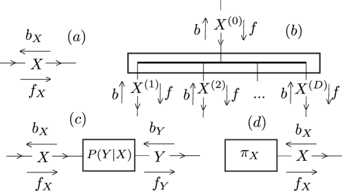
For a variable $X$ (Figure 1(a)) that takes values in the discrete alphabet ${\cal X}=\{\xi_{1},\xi_{2},\ldots,$ $\xi_{d_{X}}\}$, forward and backward messages are in function form $b_{X}(\xi_{i})$ and $f_{X}(\xi_{i})$, $i=1:d_{X}$ and in vector form ${\bf b}_{X}=(b_{X}(\xi_{1}),b_{X}(\xi_{2}),\ldots,b_{X}(\xi_{d_{X}}))^{T}$ and ${\bf f}_{X}=(f_{X}(\xi_{1}),f_{X}(\xi_{2}),\ldots,f_{X}(\xi_{d_{X}}))^{T}$. All messages are proportional ($\propto$) to discrete distributions and may be normalized to sum to one.

Comprehensive knowledge about $X$ is contained in the posterior distribution $p_{X}$ obtained through the product rule, $p_{X}(\xi_{i})\propto f_{X}(\xi_{i})b_{X}(\xi_{i})$, $i=1:d_{X}$, in function form, or ${\bf p}_{X}\propto{\bf f}_{X}\odot{\bf b}_{X}$, in vector form, where $\odot$ denotes the element-by-element product. The result of each product is proportional to a distribution and can be normalized to sum one (it is a good practice to keep messages normalized to avoid poorly conditioned products).

The replicator (or diverter) (Figure 1(b)) represents the equality constraint with the variable $X$ replicated ($D+1$) times. Messages for incoming and outgoing branches carry different forward and backward information. Messages that leave the block are obtained as the product of the incoming ones: $b_{X^{(0)}}(\xi_{i})\propto\prod_{j=1}^{D}b_{X^{(j)}}(\xi_{i})$; $f_{X^{(k)}}(\xi_{i})\propto f_{X^{(0)}}(\xi_{i})\prod_{j=1,j\neq k}^{D}b_{X^{(j)}}(\xi_{i})$, $k=1:D$, $i=1:d_{x}$ in function form. In vector form: ${\bf b}_{X}^{(0)}\propto\odot_{j=1}^{D}{\bf b}_{X}^{(j)}$; ${\bf f}_{X}^{(k)}\propto{\bf f}_{X}^{(0)}\odot_{j=1,j\neq k}^{D}{\bf b}_{X}^{(j)}$, $k=1:D$.

The SISO block (Figure 1(c)) represents the conditional probability matrix of $Y$ given $X$. More specifically if $X$ takes values in the discrete alphabet ${\cal X}=\{\xi_{1},\xi_{2},...,\xi_{d_{X}}\}$ and $Y$ in ${\cal Y}=\{\upsilon_{1},\upsilon_{2},...,\upsilon_{d_{Y}}\}$, $P(Y|X)$ is the $d_{X}\times d_{Y}$ row-stochastic matrix $P(Y|X)=[Pr\{Y=\upsilon_{j}|X=\xi_{i}\}]_{i=1:d_{X}}^{j=1:d_{Y}}=[\theta_{ij}]_{i=1:d_{X}}^{j=1:d_{Y}}$. Outgoing messages are: $f_{Y}(\upsilon_{j})\propto\sum_{i=1}^{d_{X}}\theta_{ij}f_{X}(\xi_{i})$; $b_{X}(\xi_{i})\propto\sum_{j=1}^{d_{Y}}\theta_{ij}b_{Y}(\upsilon_{j})$, in function form. In vector form: ${\bf f}_{Y}\propto P(Y|X)^{T}{\bf f}_{X}$; ${\bf b}_{X}\propto P(Y|X){\bf b}_{Y}$.

The source block in Figure 1(d) is the termination for the independent source variable $X$. More specifically $\pi_{X}$ is the $d_{X}$-dimensional prior distribution on $X$ with the outgoing message $f_{X}(\xi_{i})=\pi_{X}(\xi_{i}),i=1:d_{X}$ in function form, or ${\bf f}_{X}={\boldsymbol{\pi}}_{X}$ in vector form. The backward message ${\bf b}_{X}$ coming from the network can be combined with the forward ${\bf f}_{X}$ for final posterior on $X$.

For the reader not familiar with the factor graph framework, it should be emphasized that the above rules are rigorous translation of Bayes’ theorem and marginalization. For a more detailed review, refer to our recent works (Palmieri, 2013), (Buonanno and Palmieri, 2014) (or to the classical papers (Loeliger, 2004) (Kschischang et al., 2001)).

Parameters (probabilities) in the SISO and the source blocks must be learned from examples solely on the backward and forward flows available locally. We set the learning problem as an EM algorithm to maximize global likelihood (Palmieri, 2013). Focusing on a specific SISO block, if all the other network parameters have been fixed, maximization of global likelihood translates in the local problem from examples $({\bf f}_{X[n]},{\bf b}_{Y[n]})$, $n=1,...,N_{e}$

$$\left\{\begin{array}[]{l}\min_{\theta}~{}~{}-\sum_{n=1}^{N_{e}}\log\left({\bf f}_{X[n]}^{T}~{}\theta~{}{\bf b}_{Y[n]}\right),\\ \theta~{}~{}~{}~{}{\rm row-stochastic}.\end{array}\right.$$ (1)

After adding a stabilizing term to the cost function and applying KKT conditions we obtain the following algorithm (Palmieri, 2013).

Algorithm 1 Learning Algorithm for SISO block

1:procedure Learning Algo

2:     Initialize $\theta$ to uniform rows: $\theta=(1/d_{Y}){\bf 1}_{d_{X}\times d_{Y}}$

3:     for $i=1:d_{X}$ do

4:         $ftmp(i)=\sum_{n=1}^{N_{e}}f_{X[n]}(i)$

5:     end for

6:     for $it=1:N_{it}$ do

7:         for $n=1:N_{e}$ do

8:              $den(n)={\bf f}_{X[n]}^{T}\theta{\bf b}_{Y[n]}$

9:         end for

10:         for $i=1:d_{X}$ do

11:              for $j=1:d_{Y}$ do

12:                  $tmpSum=\sum_{n=1}^{N_{e}}\frac{f_{X[n]}(i)b_{Y[n]}(j)}{den(n)}$

13:                  $\theta_{ij}\leftarrow\frac{\theta_{ij}}{ftmp(i)}\cdot tmpSum$,

14:              end for

15:         end for

16:         Row-normalize $\theta$

17:     end for

18:end procedure(We have used the shortened notation $f_{X[n]}(\xi_{i})=f_{X[n]}(i)$, $b_{Y[n]}(v_{j})=b_{Y[n]}(j)$).

In Algorithm 1 there are three main blocks and the complexity in the worst case is $O(N_{e}\cdot d_{X}\cdot d_{Y}\cdot N_{it})$. The algorithm is a fast multiplicative update with no free parameters. The iterations usually converge in a few steps and the presence of the normalizing factors makes the algorithm numerically very stable. The algorithm has been discussed and compared to other similar updates in (Palmieri, 2013).

The updates for the source block are immediate if we set the forward messages ${\bf f}_{X[n]}$ to a uniform distribution and consider any row of $\theta$ to be the target distribution.

4 Bayesian Clustering

For the architectures that will follow, the basic building block is the Latent-Variable Model (LVM) shown in Figure 2. At the bottom of each LVM there are $N\cdot M$ variables $X[n,m]$, $n=1:N$, $m=1:M$ that belong to a finite alphabet $\mathcal{X}=\{\xi_{1},\xi_{2},\ldots,\xi_{d_{X}}\}$. The variables are organized here on a plane (as an image) because they will compose the layers of a multi-layer architecture. The $N\cdot M$ variables code multiple discrete labels, that in the application that follows take values in the same alphabet, but they could easily have different cardinalities if we need to fuse information coming from different sources (the combination of the heterogeneous variables is one of the most powerful peculiarities of the FGrn paradigm). Generally the complexity of the whole system increases with the cardinality of the alphabets.

The $N\cdot M$ bottom variables are connected to one Hidden (Latent) Variable $S$, that belongs to the finite alphabet $\mathcal{S}=\{\sigma_{1},\sigma_{2},\ldots,\sigma_{d_{S}}\}$. The replicator block of Figure 1(b) is drawn here as a box as it will be a patch of the upper plane of each layer in our architecture. Each connection to the bottom layer is a SISO block that represents the $d_{S}\times d_{X}$ row-stochastic probability matrix

$$P(X[n,m]|S)=\begin{bmatrix}P(X[n,m]=\xi_{1}|S=\sigma_{1})\ \ldots\ P(X[n,m]=\xi_{d_{X}}|S=\sigma_{1})\\ P(X[n,m]=\xi_{1}|S=\sigma_{2})\ \ldots\ P(X[n,m]=\xi_{d_{X}}|S=\sigma_{2})\\ \vdots\\ P(X[n,m]=\xi_{1}|S=\sigma_{d_{S}})\ \ldots\ P(X[n,m]=\xi_{d_{X}}|S=\sigma_{d_{S}})\\ \end{bmatrix}$$

The system is drawn as a generative model with the arrows pointing down assuming that the source is variable $S$ and the bottom variables are its children. This architecture can be seen also as a Mixture of Categorical Distributions (Koller and Friedman, 2009). Each element of the alphabet $\mathcal{S}$ represents a ”Bayesian cluster” for the $N\cdot M$ dimensional stochastic image, ${\bf X}=[X[n,m]]_{n=1:N}^{m=1:M}$ (similar to the Naive Bayes classifier (Barber, 2012)). Essentially each bottom variable is independent from the others given the Hidden Variable (Koller and Friedman, 2009). One way to visualize the model is to imagine drawing a sample: for each data point we draw a cluster index $s\in\mathcal{S}=\{\sigma_{1},\sigma_{2},\ldots,\sigma_{d_{S}}\}$ according to the prior distribution $\pi_{S}$. Then for each $n=1:N$, $m=1:M$, we draw $x[n,m]\in\{\xi_{1},\xi_{2},\ldots,\xi_{d_{X}}\}$ according to $P(X[n,m]|S=s)$.

Figure 2: A ($N\cdot M$) - tuple with the Latent Variable as a Bayesian graph (left) and as a Factor Graph in Reduced Normal Form (right). Only the first SISO block has been explicitly described.

We can perform exact inference simply by letting the messages propagate and collecting the results. Information can be injected at any node and inference can be obtained for each variable using the usual sum-product rules. For each SISO block of Figure 2 the incoming messages ($b_{X}$ and $f_{S}$) and the outgoing messages ($f_{X}$ and $b_{S}$) flow simultaneously following the rules outlined in the previous section (sum rule). In the replicator block, incoming messages from all directions are combined with product rule to produce outgoing messages. We can imagine the replicator block as acting like a bus where information is combined and diverted towards the connected branches.

Handling information in the Bayesian architecture is very flexible since each variable $X[n,m]$ corresponds to a pair of messages. The backward message coming from below is propagated upward towards the latent variable and, through the diverter, towards the sibling branches downwards to the forward messages at the terminations. At the same time the latent variable, fed through its forward message from above, sends information downward through the diverter.

5 Multi-layer FGrn

In this work we build a multilayer structure as in Figure 3(a) on top of a bottom layer of random variables. They can be pixels of an image, a feature map, or more generally a collection of spatially distributed discrete variables. In the following we refer to the bottom variables as the Image.

The architecture that lays on top of the Image is the quadtree. In Figure 3 the cyan spheres are the image variables and the other ones (red, green and blue) are the embedding (latent or hidden) variables of the LVM blocks. In Figure 3(b) the same architecture is represented as a FGrn.

Figure 3: (a) The quadtree architecture; (b) Reduced Normal Factor Graph representation of the quadtree architecture with 4 layers (0-3).

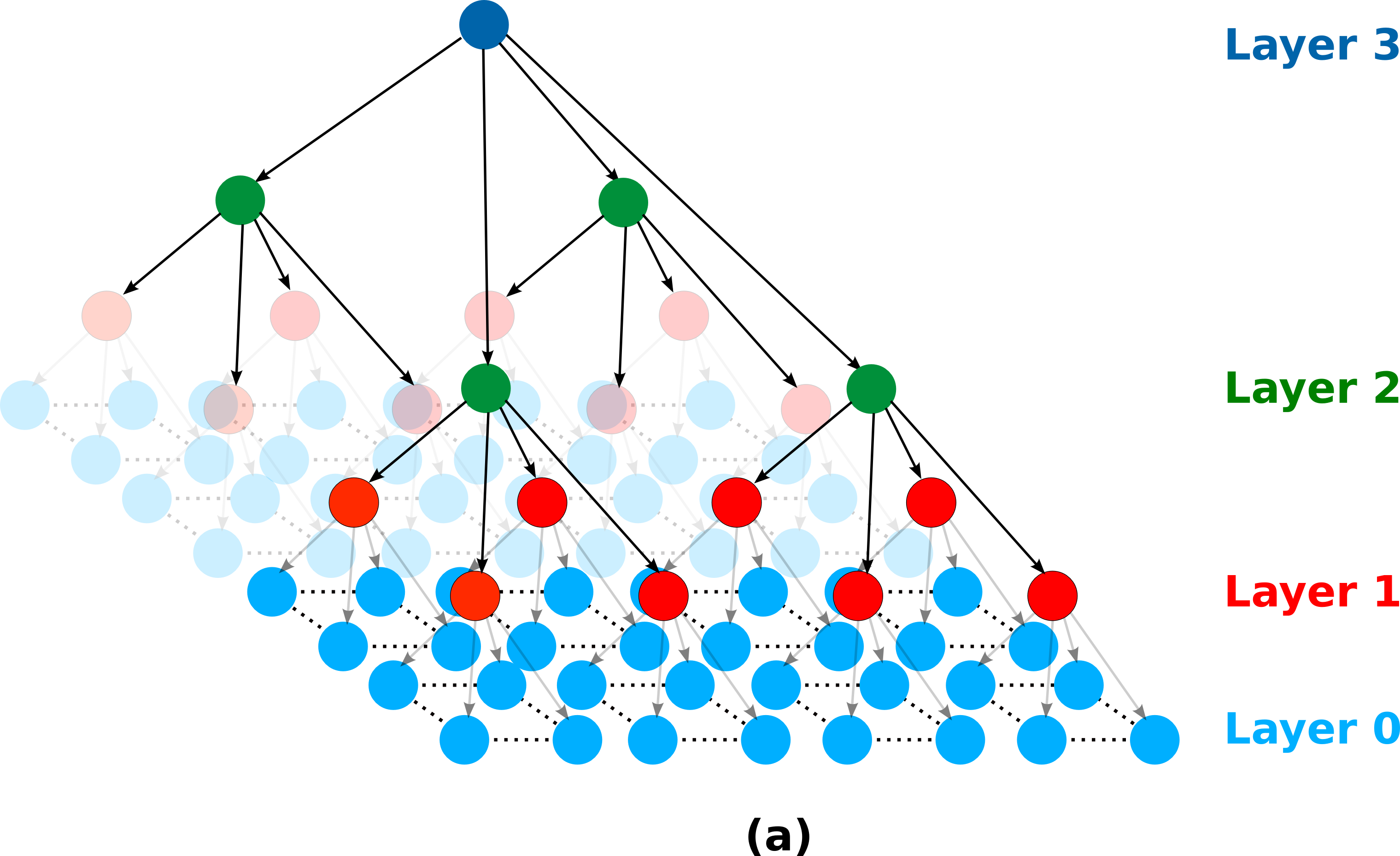
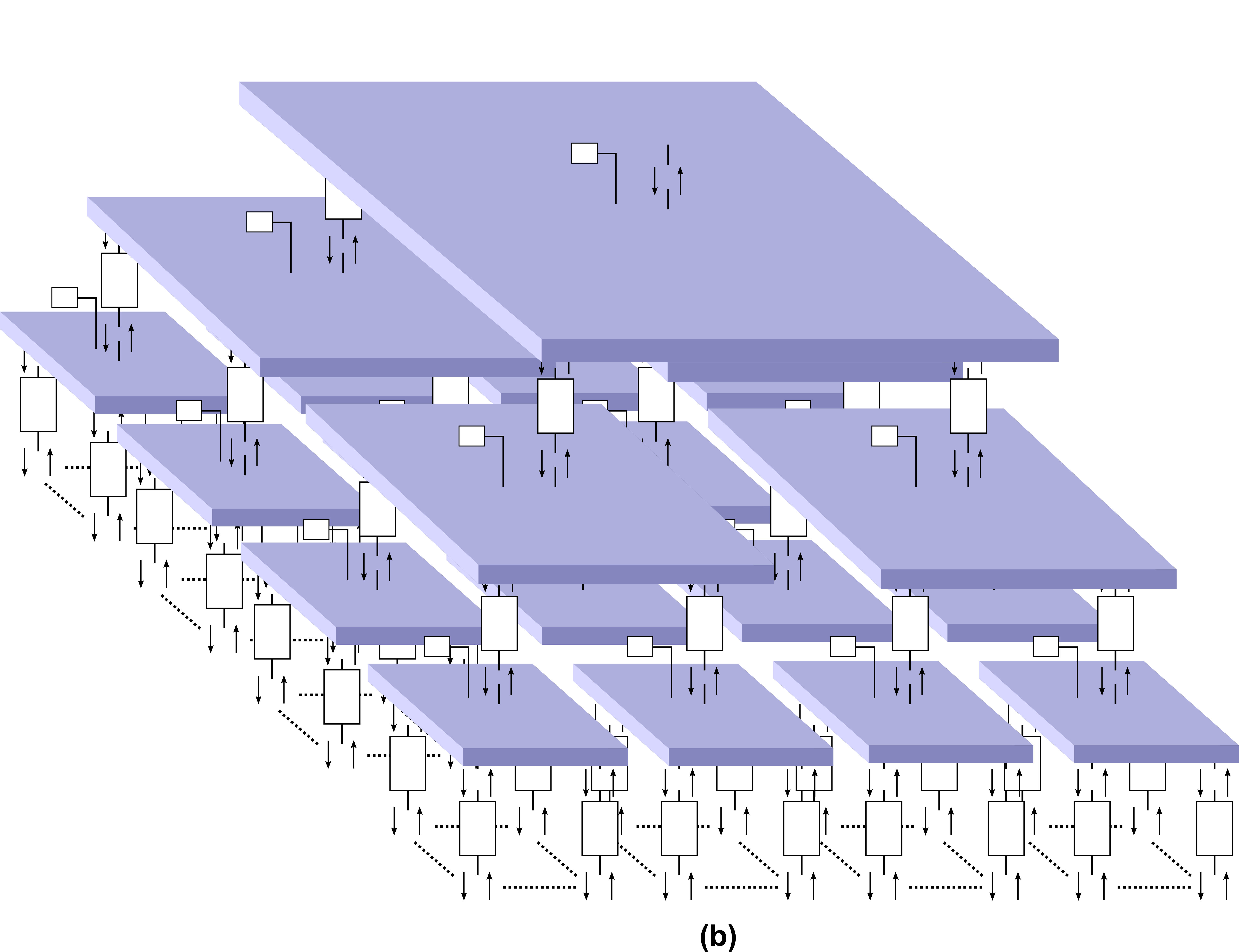
A network with $L+1$ levels (Layer $0,\ldots,$Layer $L$) covers a bottom image (Layer $0$) $S_{0}[n,m]$ $n=1:N\cdot 2^{L-1}$, $m=1:M\cdot 2^{L-1}$, subdivided in $(2^{L-1})\cdot(2^{L-1})$ image patches of dimension $(N\cdot M)$. At Layer $1$ each patch is managed by one of the latent variables $S_{1}[n,m]$, $n=1:2^{L-1}$, $m=1:2^{L-1}$ of cardinality of $d_{S_{1}}$. At Layer $2$ each latent variable $S_{2}[n,m]$, $n=1:2^{L-2}$, $m=1:2^{L-2}$ with dimension $d_{S_{2}}$, is connected to 4 variables of Layer $1$. Similarly climbing the tree in quadruples up to the root with variable $S_{L}$.

Messages travel within each layer (among the subset of LVM variables) and with the layers above and below (within the connected patches and quadruples). The architecture builds a hierarchical Bayesian clustering of the information that is exchanged across different representation scales.

5.1 Inference Modes

If the network parameters have been learned, the system can be used in the following main inference modes:

Generative: A latent variable $S_{i}[n,m]$ is fixed to a value $\sigma^{i}_{k}$, i.e. its forward distribution is a delta $f_{S_{i}}(s)=\delta(s-\sigma^{i}_{k})$, $\sigma^{i}_{k}\in\mathcal{S}_{i}=\{\sigma^{i}_{1},\sigma^{i}_{2},\ldots,\sigma^{i}_{d_{S_{i}}}\}$. After message propagation downward the forward messages at the terminal variables $S_{0}[n,m]$ in the cone subtended by $S_{i}$ reveal the $k$-th ”hierarchical conditional distribution” associated to $S_{i}$. This generation could be done on Layer 1 to check for clusters in the image patches, or at higher layers to visualize the coding role of the various hierarchical representations.

Of course propagation can be done from a generic node also upward with a backward delta distribution. The complete upward and downward flow, up to the tree root and down to the other terminations, would reveal the role of that specific node in the representation memorized in the system (a sort of impulse response).

Encoding: The image ${\bf S_{0}}=S_{0}[n,m]$, $n=1:N\cdot 2^{L-1}$, $m=1:M\cdot 2^{L-1}$, is known and the values of the bottom variables are injected in the backward messages as delta distributions. After all messages have been propagated for a number of steps equal to the network diameter (in this case $2\cdot L+1$), at each hidden variable $S_{i}[n,m]$, $i=1,\ldots,L$, $n=1:2^{L-i}$, $m=1:2^{L-i}$, we find the contribution of the observations to the posterior for $S_{i}[n,m]$. The exact posterior on $S_{i}[n,m]$ is obtained as the normalized product of forward and backward messages. Each hidden variable represents one of the components of the (soft) code of the image.

Pattern Completion: Only some of the bottom variables of ${\bf S}_{0}$ are known, i.e. their backward messages are deltas. For the unknown variables the backward messages are uniform distributions. In this modality, after at least $2\cdot L+1$ steps, the network returns forward messages at the terminal variables that try to complete the pattern (associative recall, or content-addressed memory).

Error Correction: Some of the bottom variables of ${\bf S}_{0}$ are known softly, or wrongly, with smooth distributions, or delta functions respectively. After at least $2\cdot L+1$ steps of message propagation, the network produces forward messages at the terminations that attempt to correct the distributions, or reduce the uncertainty. The posterior distributions at the terminal variables $S_{0}[n,m]$ are obtained as the normalized product of forward and backward messages.

Before propagation, all messages that do not correspond to evidence, are initialized to uniform distributions.

5.2 Learning

The parameters contained in the FG are learned from a training set of $T$ images ${\bf S}_{0}^{1},\ldots,{\bf S}_{0}^{T}$.

We assume that within each layer the LVM blocks share the same parameters. This is a standard shift-invariance assumption that most deep belief networks make.

Given a basic patch of dimension $N\cdot M$ pixels and a network with $L+1$ levels (Layer $0,\ldots,$Layer $L$), for Layer $1$ we need to learn $N\cdot M$ matrices $P(S_{0}[n,m]|S_{1})$ (one per pixel) each one having sizes $d_{S_{1}}\times d_{S_{0}}$ and the $d_{S_{1}}$-dimensional prior vector $\Pi_{S_{1}}$.

For Layers $2$ to $L$ we need to learn 4 matrices $P(S_{i-1}[n,m]|S_{i})$ having sizes $d_{S_{i}}\times d_{S_{i-1}}$ and the $d_{S_{i}}$-dimensional prior vector $\Pi_{S_{i}}$.

A generic image of the training set is subdivided in $L$-Level patches of dimension $(2^{L-1}\cdot N)\cdot(2^{L-1}\cdot M)$ pixels. Each $L$-Level patch is subdivided in $2\cdot 2$ $(L-1)$-Level patches, $2^{2}\cdot 2^{2}$ $(L-2)$-Level patches and so on until to obtain $(2^{L-1})\cdot(2^{L-1})$ patches of dimension $(N\cdot M)$ pixels at Layer 1 ($0$-Level and $1$-Level patches are the same).

The examples, subdivided in $1st$-Level patches, are presented to the termination of the LVM in Fig. 2 as sharp backward distributions for a fixed number of steps (epochs). All SISO blocks and the source block adapt their parameters using an iterative Maximum Likelihood Algorithm (Palmieri (2013)) outlined in Section 3.

Once the Layer $1$ is learned, the $2nd$-Level patches are used to learn Layer $2$ constructed combining 4 LVMs of Layer $1$ and the process goes on, building deeper and deeper network and considering larger and larger patches.

At the end of the learning phase the matrices are frozen and used in one of the inference modes described before on the same training set to check for accuracy and on a test set to check for generalization.

More specifically, learning is off-line and it is composed by the following steps for an architecture of $L+1$ layers and a basic patch dimension of $N\cdot M$ pixels:

1. We randomly select $P$ $L$-Level Patches from each image in the Training Set composed by $T$ images. Therefore, in the learning phase, we have $T\cdot P$ $L$-Level patches that are subdivided in Patches of the lower levels until to obtain $1st$-Level Patches;

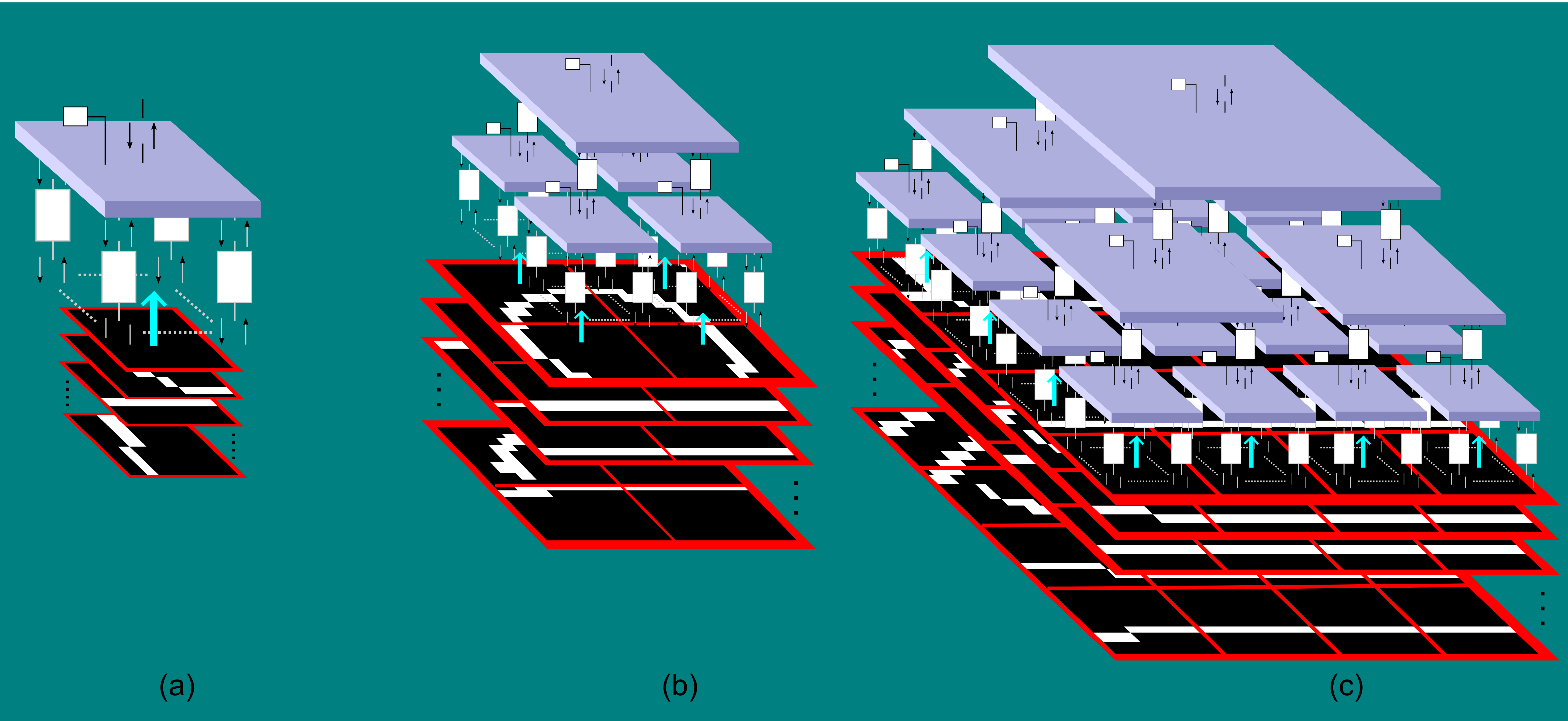
2. The $T\cdot P\cdot(2^{L-1}\cdot 2^{L-1})$ $1st$-Level Patches of $(N\cdot M)$ pixels are injected at the bottom of the LVM and the parameters are learned (Figure 4(a));

3. A new $3$-Layers network (0-2) is built replicating $2\cdot 2$ times the LVM block learned above and connecting their Hidden Variables with another LVM Block;

4. The $T\cdot P\cdot(2^{L-2})\cdot(2^{L-2})$ Patches of $(2\cdot N)\cdot(2\cdot M)$ pixels are injected at the bottom of the new $3$-Layers network and the backward messages at the top of Layer $1$ are used to learn the LVM block at Layer $2$ (Figure 4(b));

5. A new $4$-Layers network (0-3) is built replicating for $2^{2}\cdot 2^{2}$ times the LVM block learned at step 2 and for $2\cdot 2$ times the LVM block learned at step 4 and connecting their Hidden Variables to another LVM Block;

6. The $T\cdot P\cdot(2^{L-3})\cdot(2^{L-3})$ Patches of $(2^{2}\cdot N)\cdot(2^{2}\cdot M)$ pixels are propagated in the Layer $1$ and Layer $2$ and the backward messages at the top of the Layer $2$, are used to learn the LVM block at Layer $3$ (Figure 4(c));

7. The same progression is applied to all the other layers, extending the number of LVM block replicas to cover the dimension of the current-Level Patch.

Figure 4: Learning Steps for a 4-Layers Architecture: (a) Learning Layer $1$; (2) Learning Layer $2$; (3) Learning Layer $3$

6 Simulations

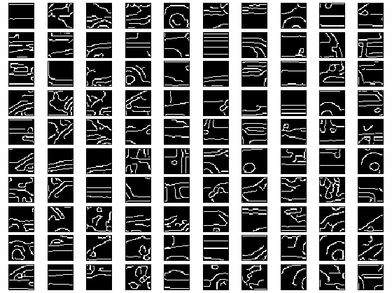
In this set of simulations we have taken 50 car images from Caltech101 Dataset. Each image is cropped, filtered with an anisotropic diffusion algorithm (Kovesi ), whitened and finally filtered with a Canny filter in order to obtain images with only the car borders. Our input alphabet is binary ($d_{S_{0}}=2$). From the 50 filtered images a set of 500 image patches of $32\cdot 32$ pixels are randomly extracted. A small subset is shown in Fig. 5.

6.1 Learning

The steps for the learning phase are described in the previous and use the following variables: $P=10$, $T=50$, $N=8$, $M=8$, $L=3$, $d_{S_{0}}=2$, $d_{S_{1}}=100$, $d_{S_{2}}=300$, $d_{S_{3}}=300$.

Figure 5: Some images from the Training Set

6.2 Inference

Once the matrices have been learned we use the network in various inference modes:

Generative mode: We obtain forward distributions at the bottom terminations by injecting at the top of the various structures a delta distribution (the images in gray scale show at each pixel the probability on one of the two symbols). More specifically, for visualizing the conditional distributions corresponding to Layer $1$ we consider only the Latent Model in Figure 2; for Layer $2$ we consider the $3$-Layers architecture composed by 4 LVM Blocks connected to one LVM Block; for Layer $3$ we consider the complete architecture. Figures 6, 7 and 8 show respectively the forward distributions generated injecting deltas at Layers $1$, $2$ and $3$.

Figure 6: Forward distributions learned at the first level. Dimension of the Embedding Space: 100

Figure 7: 100 of 300 forward distributions learned at the second level. Dimension of the Embedding Space: 300

Figure 8: 100 of 300 forward distributions learned at the third level. Dimension of the Embedding Space: 300

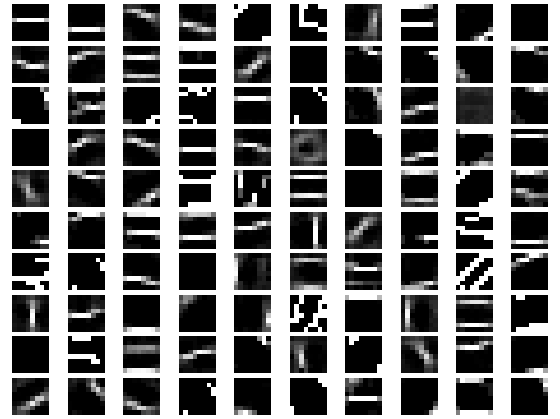
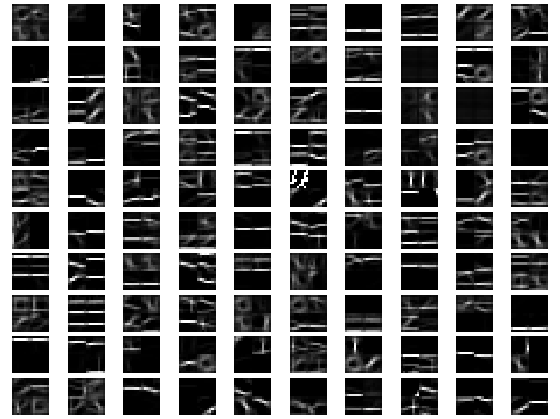
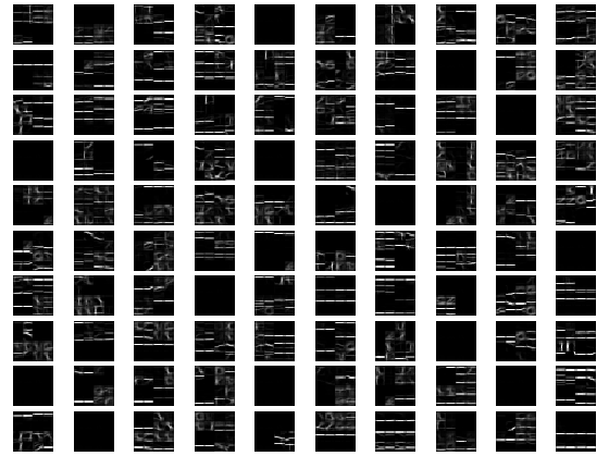
The network has stored quite well the complex structures. The forward distributions from Layer 1 represent simple orientation patterns similar to the ones that the early human visual system responds to. At Layer 3 the distributions reflect the combined representations stored at larger scales.

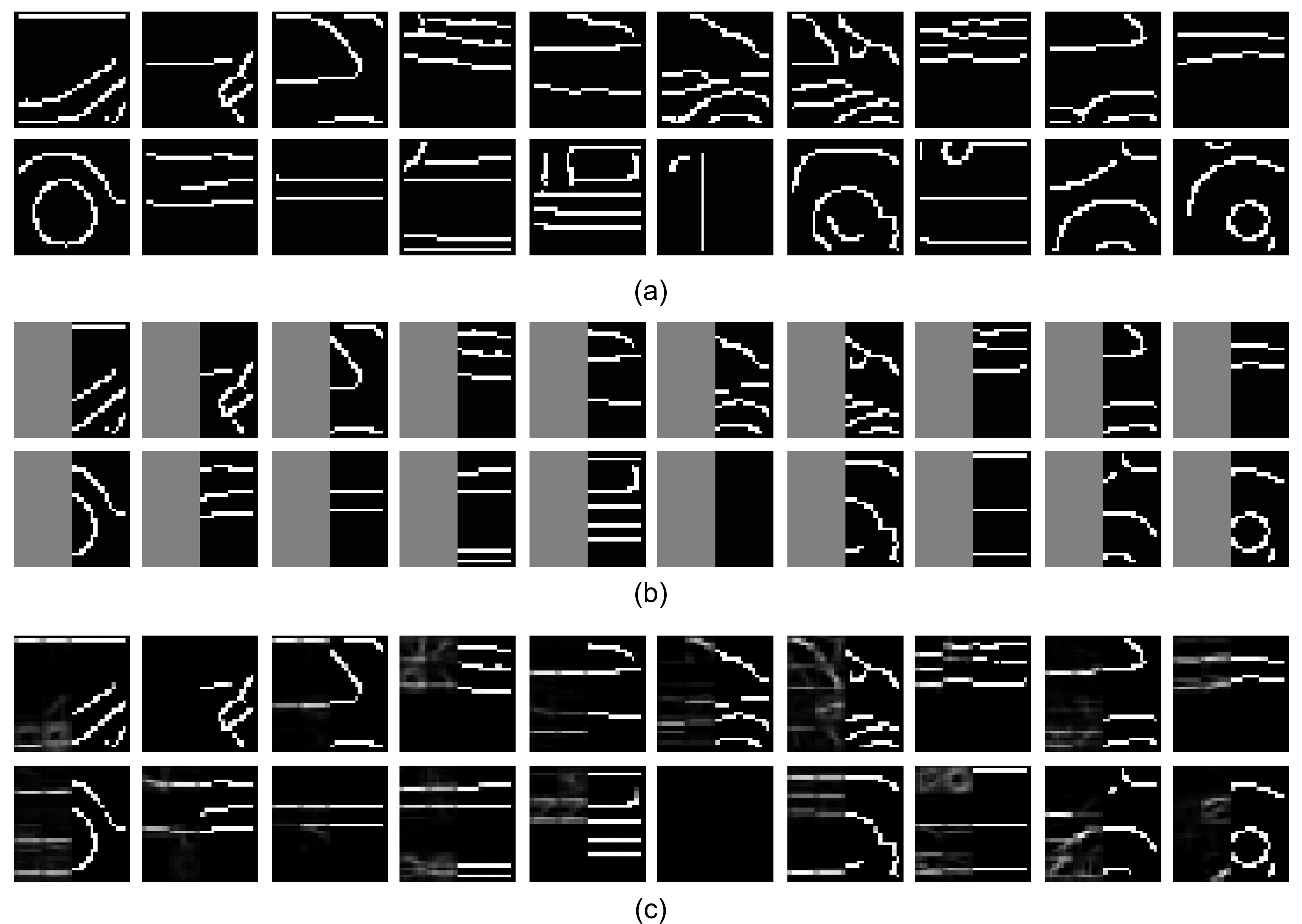
Pattern Completion: In these experiments we have used the architecture as an associative memory that is queried with incomplete patterns and responds with the information stored during the learning phase. Figure 9(a) shows 20 patches extracted from Training Set. Before the injection at the bottom of the network, a considerable amount of pixels (16 patches on a total of 32 patches) has been erased (Figure 9(b)), i.e. the delta backward distribution is replaced with an uniform distribution. Figure 9(c) shows the forward distributions for the same images after message propagation. The network is able to resolve quite well most of the uncertainties using the stored information.

Figure 9: Completion of Patterns obtained from the Training Set. (a) Original image, (b) Image with many erasures (in gray), (c) Image inferred by the network

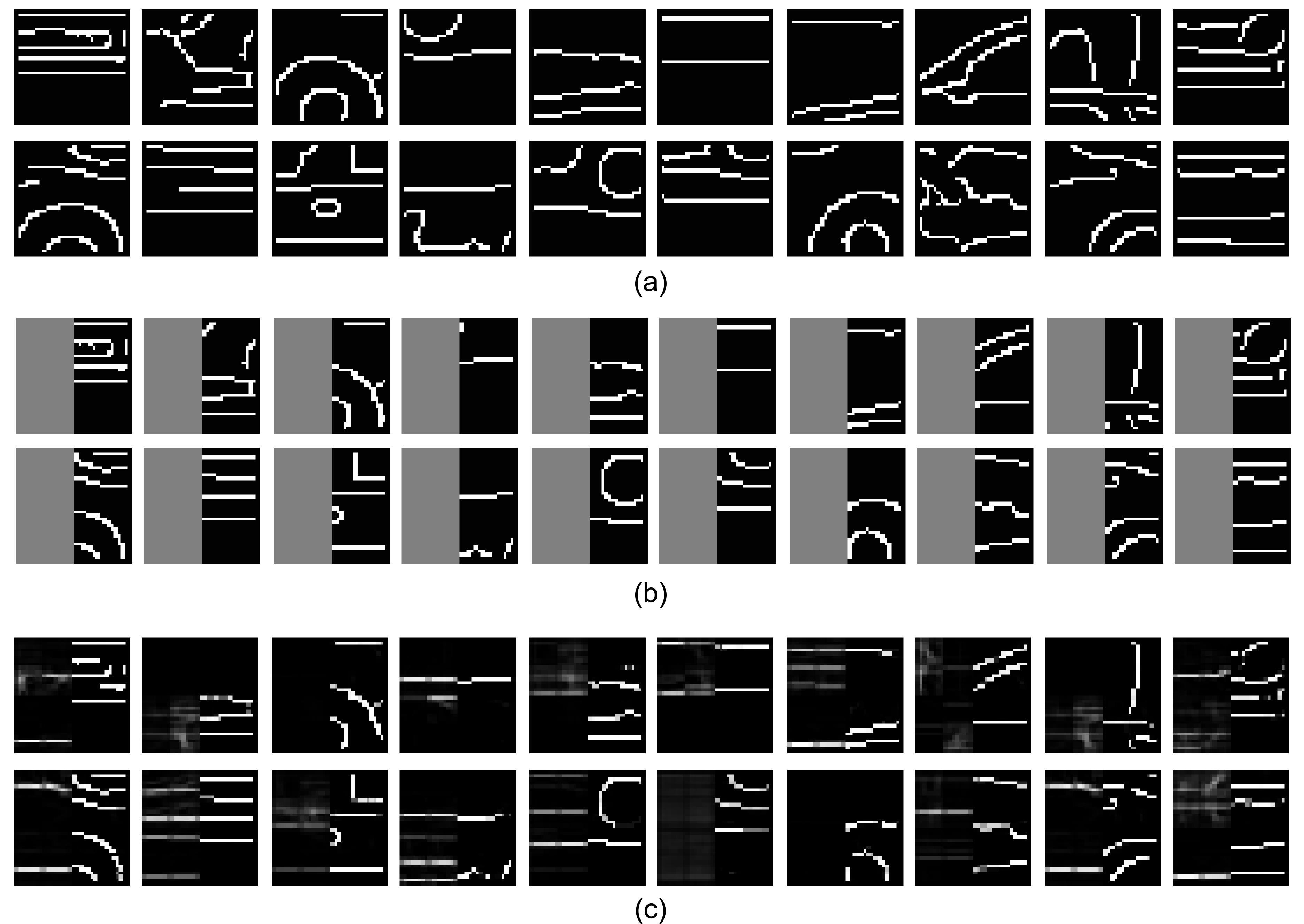
The same experiment of Pattern Completion has been repeated with patches extracted from the Test Set (patterns that the network has never seen before). The result is obviously worse as shown in Figure 10, but it’s worthy to note that the network succeeds quite well in completing most of the shapes in applying the learned knowledge (test for generalization). Cross-validation can be easily applied to determine the most appropriate embedding spaces sizes for best generalization.

Figure 10: Completion of Patterns obtained from the Test Set. (a) Original image, (b) Image with some erasures (in gray), (c) Image inferred by the network.

7 Discussion and Conclusions

From the results presented above we have demonstrated that the paradigm of the FGrn can be successfully applied to build deep architectures. The layers retain the information about the clusters contained in the data and build a hierarchical internal representation. Each layer successfully learns to compose the objects made available from the lower layers.

We have chosen the border of car images extracted from Caltech101 because we wanted to see if the paradigm was suitable for patching together the salient structures of an object. Other experiments have been performed on characters and different patterns revealing very similar results.

We believe that the FGrn paradigm constitutes a promising addition to the various proposals for deep networks that are appearing in the literature. It can provide great flexibility and modularity. The network can be easily extended by introducing new and different (in cardinality and in type) variables. Prior knowledge and supervised information can be inserted at any of the scales: new “label variables” can be added in one or more of the diverter junctions and let learning take care of parameter adaptation. Results of these mixed supervised/unsupervised architectures are under way and will be reported elsewhere.

The computational complexity issue that clearly emerges from this paradigm, specially when the embedding variables have large dimensionality and when image pixels are non binary, is being exploited for parallel implementations. Since both belief propagation and learning are totally local, they can be implemented with distributed hardware or parallelized processes. Some studies have been carried out for other deep network frameworks (Liang et al., 2009), (Silberstein et al., 2008), (Ma et al., 2012)) and we are confident that similarly the FGrn paradigm may present new interesting opportunities to approach some of the most challenging tasks in computer vision.

References

- Barber (2012) D. Barber. Bayesian Reasoning and Machine Learning. Cambridge University Press, 2012.
- Beal (2003) M. J. Beal. Variational Algorithms for Approximate Bayesian Inference. PhD thesis, University of London, 2003.
- Bengio et al. (2007) Y. Bengio, P. Lamblin, D. Popovici, and H. Larochelle. Greedy layer-wise training of deep networks. In B. Schölkopf, J. Platt, and T. Hoffman, editors, Advances in Neural Information Processing Systems 19, pages 153–160. MIT Press, Cambridge, MA, 2007.
- Bengio and Delalleau (2011) Yoshua Bengio and Olivier Delalleau. On the expressive power of deep architectures. In Jyrki Kivinen, Csaba Szepesvári, Esko Ukkonen, and Thomas Zeugmann, editors, Algorithmic Learning Theory, volume 6925 of Lecture Notes in Computer Science, pages 18–36. Springer Berlin Heidelberg, 2011. ISBN 978-3-642-24411-7.
- Bengio et al. (2012) Yoshua Bengio, Aaron Courville, and Pascal Vincent. Representation learning: A review and new perspectives, 2012. URL http://arxiv.org/abs/1206.5538. cite arxiv:1206.5538.
- Bengio et al. (2014) Yoshua Bengio, Ian J. Goodfellow, and Aaron Courville. Deep learning. Book in preparation for MIT Press, 2014. URL http://www.iro.umontreal.ca/ bengioy/dlbook.
- Bishop (1999) Christopher M. Bishop. Latent variable models. In Learning in Graphical Models, pages 371–403. MIT Press, 1999.
- Bouman and Shapiro (1994) Charles A. Bouman and Michael Shapiro. A multiscale random field model for bayesian image segmentation. IEEE Transactions on Image Processing, 3(2):162–177, 1994.
- Boykov et al. (1999) Yuri Boykov, Olga Veksler, and Ramin Zabih. Fast approximate energy minimization via graph cuts. IEEE Transactions on Pattern Analysis and Machine Intelligence, 23:2001, 1999.
- Buonanno and Palmieri (2014) A. Buonanno and F. A. N. Palmieri. Simulink implementation of belief propagation in normal factor graphs. In Proceedings of the 24th Workshop on Neural Networks, WIRN 2014, May 15-16, Vietri sul Mare, Salerno, Italy, 2014.
- Cheeseman and Stutz (1996) Peter Cheeseman and John Stutz. Bayesian classification (autoclass): Theory and results, 1996.
- Choi et al. (2011) M. J. Choi, V. Y. F. Tan, A. Anandkumar, and A. S. Willsky. Learning latent tree graphical models. Journal of Machine Learning Research, 12:1771–1812, 2011.
- Coates and Ng (2012) Adam Coates and Andrew Y. Ng. Learning feature representations with k-means. In Grégoire Montavon, Genevieve B. Orr, and Klaus-Robert Müller, editors, Neural Networks: Tricks of the Trade (2nd ed.), volume 7700 of Lecture Notes in Computer Science, pages 561–580. Springer, 2012. ISBN 978-3-642-35288-1.
- Dileep (2008) G. Dileep. How the brain might work: A hierarchical and temporal model for learning and recognition. PhD thesis, 2008.
- Forney (2001) G. D. Forney. Codes on graphs: Normal realizations. IEEE Transactions on Information Theory, 47:520–548, 2001.
- Frean (2008) Marcus Frean. Inference in loopy graphs. Class Notes in Machine Learning COMP 431, 2008.
- Gelfand and Smith (1990) Alan E. Gelfand and Adrian F. M. Smith. Sampling-Based Approaches to Calculating Marginal Densities. Journal of the American Statistical Association, 85(410):398–409, 1990. ISSN 01621459. doi: 10.2307/2289776. URL http://dx.doi.org/10.2307/2289776.
- Geman and Geman (1984) Stuart Geman and D. Geman. Stochastic relaxation, gibbs distributions, and the bayesian restoration of images. Pattern Analysis and Machine Intelligence, IEEE Transactions on, PAMI-6(6):721–741, Nov 1984. ISSN 0162-8828. doi: 10.1109/TPAMI.1984.4767596.
- Hawkins (2004) Jeff Hawkins. On Intelligence (with Sandra Blakeslee). Times Books, 2004. URL http://www.amazon.com/Intelligence-Jeff-Hawkins/dp/0805074562.
- Hinton and Salakhutdinov (2006) G E Hinton and R R Salakhutdinov. Reducing the dimensionality of data with neural networks. Science, 313(5786):504–507, July 2006. doi: 10.1126/science.1127647.
- Hinton et al. (2006) Geoffrey E. Hinton, Simon Osindero, and Yee Whye Teh. A fast learning algorithm for deep belief nets. Neural Computation, 18(7):1527–1554, 2006.
- Jordan et al. (1999) Michael I. Jordan, Zoubin Ghahramani, Tommi Jaakkola, and Lawrence K. Saul. An introduction to variational methods for graphical models. Machine Learning, 37:183–233, 1999.
- Koller and Friedman (2009) Daphne Koller and Nir Friedman. Probabilistic Graphical Models: Principles and Techniques. MIT Press, 2009.
- (24) P. D. Kovesi. MATLAB and Octave functions for computer vision and image processing. Centre for Exploration Targeting, School of Earth and Environment, The University of Western Australia. Available from: http://www.csse.uwa.edu.au/pk/research/matlabfns/.
- Kschischang et al. (2001) F. R. Kschischang, B.J. Frey, and H.A. Loeliger. Factor graphs and the sum-product algorithm. IEEE Transactions on Information Theory, 47:498–519, 2001.
- Laferte et al. (2000) J. M. Laferte, P. Perez, and F. Heitz. Discrete markov image modeling and inference on the quadtree. Trans. Img. Proc., 9(3):390–404, March 2000. ISSN 1057-7149. doi: 10.1109/83.826777. URL http://dx.doi.org/10.1109/83.826777.
- Lee et al. (2008) H. Lee, C. Ekanadham, and A. Ng. Sparse deep belief net model for visual area v2. In J.C. Platt, D. Koller, Y. Singer, and S. Roweis, editors, Advances in Neural Information Processing Systems 20. MIT Press, Cambridge, MA, 2008.
- Liang et al. (2009) Chia-Kai Liang, Chao-Chung Cheng, Yen-Chieh Lai, Liang-Gee Chen, and Homer H. Chen. Hardware-efficient belief propagation. In CVPR, pages 80–87. IEEE, 2009. ISBN 978-1-4244-3992-8.
- Loeliger (2004) H. A. Loeliger. An introduction to factor graphs. IEEE Signal Processing Magazine, 21(1):28 – 41, jan. 2004.
- Luettgen et al. (1993) M.R. Luettgen, W.C. Karl, A.S. Willsky, and R.R. Tenney. Multiscale representations of markov random fields. Trans. Sig. Proc., 41(12):3377–3396, December 1993. ISSN 1053-587X. doi: 10.1109/78.258081. URL http://dx.doi.org/10.1109/78.258081.
- Ma et al. (2012) Nam Ma, Yinglong Xia, and Viktor K. Prasanna. Task parallel implementation of belief propagation in factor graphs. In IPDPS Workshops, pages 1944–1953. IEEE Computer Society, 2012. ISBN 978-1-4673-0974-5.
- Mourad et al. (2013) Raphaël Mourad, Christine Sinoquet, N. L. Zhang, T. Liu, and Philippe Leray. A survey on latent tree models and applications. J. Artif. Intell. Res. (JAIR), 47:157–203, 2013.
- Murphy (2012) Kevin P. Murphy. Machine Learning: A Probabilistic Perspective (Adaptive Computation and Machine Learning series). The MIT Press, 2012. ISBN 0262018020.
- Nowak (1999) Robert D. Nowak. Multiscale hidden markov models for bayesian image analysis, 1999.
- Olshausen and Field (1996) B. A. Olshausen and D. J. Field. Emergence of simple-cell receptive field properties by learning a sparse code for natural images. Nature, 381:607–609, 1996.
- Palmieri and Buonanno (2014) F. Palmieri and A. Buonanno. Belief propagation and learning in convolution multi-layer factor graph. In Proceedings of the the 4th International Workshop on Cognitive Information Processing, Copenhagen - Denmark, 2014.
- Palmieri (2013) F. A. N. Palmieri. A comparison of algorithms for learning hidden variables in normal graphs. arXiv:1308.5576, 2013.
- Pearl (1988) J. Pearl. Probabilistic reasoning in intelligent systems: networks of plausible inference. Morgan Kaufmann Publishers Inc., San Francisco, CA, USA, 1988. ISBN 0-934613-73-7.
- Ranzato et al. (2006) Marc’Aurelio Ranzato, Christopher S. Poultney, Sumit Chopra, and Yann LeCun. Efficient learning of sparse representations with an energy-based model. In Bernhard Schölkopf, John Platt, and Thomas Hoffman, editors, NIPS, pages 1137–1144. MIT Press, 2006. ISBN 0-262-19568-2.
- Schmidhuber (2015) Jürgen Schmidhuber. Deep learning in neural networks: An overview. Neural Networks, 61(0):85 – 117, 2015. ISSN 0893-6080. doi: http://dx.doi.org/10.1016/j.neunet.2014.09.003.
- Serre and Poggio (2010) Thomas Serre and Tomaso Poggio. A neuromorphic approach to computer vision. Commun. ACM, 53(10):54–61, 2010.
- Silberstein et al. (2008) Mark Silberstein, Assaf Schuster, Dan Geiger, Anjul Patney, and John D. Owens. Efficient computation of sum-products on gpus through software-managed cache. In ICS ’08: Proceedings of the 22nd annual international conference on Supercomputing, pages 309–318, New York, NY, USA, 2008. ACM. ISBN 978-1-60558-158-3. doi: http://doi.acm.org/10.1145/1375527.1375572.
- Vincent et al. (2008) Pascal Vincent, Hugo Larochelle, Yoshua Bengio, and Pierre-Antoine Manzagol. Extracting and composing robust features with denoising autoencoders. In William W. Cohen, Andrew McCallum, and Sam T. Roweis, editors, ICML, volume 307 of ACM International Conference Proceeding Series, pages 1096–1103. ACM, 2008. ISBN 978-1-60558-205-4.
- Wainwright and Jordan (2008) Martin J. Wainwright and Michael I. Jordan. Graphical models, exponential families, and variational inference. Foundations and Trends in Machine Learning, 1(1-2):1–305, 2008.
- Willsky (2002) Alan S Willsky. Multiresolution markov models for signal and image processing. Proceedings of the IEEE, 90(8):1396–1458, 2002.
- Wolf and Gavin (2010) Christian Wolf and Gérald Gavin. Inference and parameter estimation on hierarchical belief networks for image segmentation. Neurocomput., 73(4-6):563–569, January 2010. ISSN 0925-2312. doi: 10.1016/j.neucom.2009.07.017. URL http://dx.doi.org/10.1016/j.neucom.2009.07.017.
- Xiong et al. (2007) Liang Xiong, Fei Wang, and Changshui Zhang. Multilevel belief propagation for fast inference on markov random fields. In ICDM, pages 371–380. IEEE Computer Society, 2007.
- Yedidia et al. (2005) J. Yedidia, W. Freeman, and Y. Weiss. Constructing free-energy approximations and generalized belief propagation algorithms. IEEE Transactions on Information Theory, 51:2282ÔøΩ2312, 2005.