Optimal modeling of 1D azimuth correlations in the context of Bayesian inference

Abstract

Analysis and interpretation of spectrum and correlation data from high-energy nuclear collisions is currently controversial because two opposing physics narratives derive contradictory implications from the same data—one narrative claiming collision dynamics is dominated by dijet production and projectile-nucleon fragmentation, the other claiming collision dynamics is dominated by a dense, flowing QCD medium. Opposing interpretations seem to be supported by alternative data models, and current model-comparison schemes are unable to distinguish between them. There is clearly need for a convincing new methodology to break the deadlock. In this study we introduce Bayesian Inference (BI) methods applied to angular correlation data as a basis to evaluate competing data models. For simplicity the data considered are projections of 2D angular correlations onto 1D azimuth from three centrality classes of 200 GeV Au-Au collisions. We consider several data models typical of current model choices, including Fourier series (FS) and a Gaussian plus various combinations of individual cosine components. We evaluate model performance with BI methods and with power-spectrum (PS) analysis. We find that the FS-only model is rejected in all cases by Bayesian analysis which always prefers a Gaussian. A cylindrical quadrupole $\cos(2\phi)$ is required in some cases but rejected for 0-5%-central Au-Au collisions. Given a Gaussian centered at the azimuth origin “higher harmonics” $\cos(m\phi)$ for $m>2$ are rejected. A model consisting of Gaussian + dipole $\cos(\phi)$ + quadrupole $\cos(2\phi)$ provides good 1D data descriptions in all cases.

I Introduction

A significant and persistent problem has emerged concerning models for high-energy nucleus-nucleus (A-A) collision data from the relativistic heavy ion collider (RHIC) and the large hadron collider (LHC). Distinct classes of data models with divergent physics implications are invoked to support two narratives: a high-energy physics (HEP)/jets narrative in which the essential phenomenon is dijet production ua1 ; kll ; sarc ; hijing ; kn and a quark-gluon plasma (QGP)/flow narrative in which the essential phenomenon is a flowing dense QCD medium or QGP and dijets play no significant role perfliq1 ; perfliq2 .

The HEP/jets narrative emerges spontaneously from an analysis program based on spectrum and correlation data models derived from the observed differential structure of available data ppprd ; hardspec ; porter2 ; porter3 ; axialci ; anomalous . In contrast, models emerging from the QGP/flow narrative tend to rely on theoretical motivations coupled with data and information selection (e.g. $p_{t}$ cuts, preferred A-A centralities, ratio measures) poskvol ; 2004 ; blastwave ; trigger ; staras ; starraa . A comparison of RHIC results and interpretations is presented in Ref. review .

For example, 2D angular correlations from high-energy nuclear collisions include only a few structures common to all collisions from $p$-$p$ to central Au-Au at RHIC energies. A simple mathematical model of those structures describes almost all data accurately with no significant residual structure porter2 ; porter3 ; axialci ; anomalous . No theoretical assumptions motivated the data model. Three of the four principal model elements have been interpreted post facto as representing dijet production and projectile-nucleon dissociation jetspec ; jetspecth ; pptheory . Interpretation of the fourth element, an independent azimuth quadrupole, remains in question azimuth1 ; gluequad ; quadspec ; davehq ; davehq2 ; nov2 ; nohydro . Differential analysis of hadron $p_{t}$ spectra reveals two components modeled by simple functions ppprd ; hardspec . One component is identified with fragments from dijets described quantitatively by QCD calculations fragevo . Most spectrum and correlation structures appear to be consistent with the HEP/jets narrative. Alternative models motivated by the QGP/flow narrative include quantity $v_{2}$ [Fourier coefficient of function $\cos(2\phi)$ fitted to 1D projections of 2D angular correlations] interpreted to represent elliptic flow poskvol ; 2004 , a blast-wave spectrum model interpreted to measure radial flow blastwave , spectrum ratio $R_{AA}$ interpreted to indicate jet quenching within a dense QCD medium starraa , and dihadron correlation analysis via background subtraction interpreted to represent jet structure staras ; trigger ; tzyam . “Higher harmonic” flows have been inferred recently from azimuth distributions via Fourier-series models gunther ; luzum ; lhcharm .

The same underlying particle data are therefore characterized and interpreted with competing mathematical models applied to different data selections, variables and measured quantities. Judgments on the validity and relative merits of competing data models have relied historically on comparisons of minimum-$\chi^{2}$ values and qualitative arguments based on consistency of a given narrative across selected measured quantities. While such an approach might suffice when the underlying physical processes and models are simple, the complexity of A-A phenomenology and lack of consistent quantitative criteria have impeded progress in resolving conflicts.

To address this problem we require a formal context in which competing data models are evaluated on a statistically sound basis, and a “best” model may be selected that either does not rely on unspoken a priori physics assumptions or renders such assumptions quantifiable. We suggest that this context exists in the form of Bayesian Inference (BI) which provides both a formal mathematical framework and the necessary concepts to represent prior knowledge, evaluate candidate models for different parameter values and thereby establish value judgments on models as a whole bayes1 ; bayes2 ; bayes3 ; mackay . Each data model is rated not only by how well it describes some data or how much data it describes well, but also by the “cost” of the model in terms of complexity and parameter number (Occam penalty) and associated physical assumptions.

In this study we focus on 1D projections onto azimuth $\phi$ of 2D angular correlations reported in Ref. anomalous , currently one of the most contentious areas of RHIC/LHC data analysis. We consider several popular data models and evaluate them according to BI methods to determine whether a uniquely preferred data model can be established without recourse to a priori physics assumptions.

This article is arranged as follows: Section II presents the basics of Bayesian Inference. Section III describes Fourier power spectra (PS) and their properties. Section IV summarizes analysis methods applied to correlation data. Section V introduces the correlation data used for this study. Sections VI, VII and VIII apply BI and PS methods to azimuth projections from three centralities of 200 GeV Au-Au collisions. Section IX presents systematic-uncertainty estimates. Sections X and XI present discussion and summary. Appendices A and B consider the geometry of BI analysis and periodic peak arrays respectively.

II Bayesian inference

Bayesian Inference addresses the problem of relating parametrized model functions to available data in an optimal manner. Given specific data values the best set of parameter values for each model is determined based on the likelihood function. Several models are then compared based on each model’s evidence, an integral measure defined below. The most plausible and therefore preferred data model produces the largest evidence value.

II.1 The $\bf\chi^{2}$ measure and model fits to data

In the present study we focus on aspects of Bayesian Inference that correspond directly with the methodology of $\chi^{2}$ minimization. Given a set of $N$ data points $(x_{n},y_{n})$ with experimentally determined standard errors $\sigma_{n}$ on $y_{n}$ the conventional $\chi^{2}$ statistic evaluating the goodness of fit of model function $f(x\,|\,w)$ with $K$ parameters $w_{k}$ is

$$\chi^{2}=\sum_{n=1}^{N}\left(\frac{y_{n}-f(x_{n}\,|\,w)}{\sigma_{n}}\right)^{2}.$$ (1)

As stated in Ref. dekock14 the $\chi^{2}$ measure assumes a Gaussian distribution of data-sample fluctuations about mean values which we accept as a reasonable approximation for 1D RHIC/LHC data projections. In what follows model functions are represented by $D(w)$, a vector function mapping parameter space $w$ to data space $D$.

Most model comparisons are based on $\chi^{2}$/DoF, where the number of fit degrees of freedom (DoF) is assumed to be the number of data points $N$ minus the number of free model parameters $K$. Minimizing $\chi^{2}$ without considering the fit DoF is clearly misleading since there are infinitely many models with $K{=}N$ free parameters that might describe the same $N$ data points with $\chi^{2}=0$ jeffreys . We require a mechanism to penalize excess model parameters such that a simple few-parameter model that describes the data well may be favored over more-complex models. That mechanism exists in the form of Bayesian Inference.

II.2 Logical and rational inference

Distinction may be drawn between logical inference on the one hand, in which nominally-valid conclusions are drawn via a logical chain of argument from premises assumed to be true and rational inference on the other, in which patterns or events (i.e. data) are used to improve our understanding of the physical system, either augmenting or displacing previous understanding. Both the acquired data and the modified understanding may be uncertain to some degree as measured by probabilities. Rational inference includes induction, in which newly-acquired data are employed to formulate or refine a model, and deduction in which a fixed model is used to predict values of data not yet acquired inference .

Bayesian Inference is a formal recipe for rational inference based on Bayes’ theorem jeffreys ; jaynes . “Understanding” in this context means that reality in the form of data or data-derived quantities is well described by a parametrized model. A given set of parameter values predicts a specific set of possible data values. Previous understanding including uncertainties is represented by the prior, a probability distribution function (PDF) on possible parameter values. As new data are acquired BI provides a means to update the PDF on model parameters to effect improved understanding in the form of the posterior PDF, thereby refining the model by reducing the volume of its parameter space or falsifying the model altogether if the new data fall outside the model’s predicted data volume.

II.3 The probability chain rule and Bayes’ theorem

Bayesian Inference is based on relations among joint, conditional and marginal PDFs and related unnormalized functions distributed on data and model-parameter spaces kendall . External factors common to all models that may influence the inference process are represented by a comprehensive parameter set $Q$ suppressed below. Our notation follows that in Refs. mackay and jaynes .

A model $H$ is defined by a joint PDF $p(wD|HQ)\rightarrow p(wD|H)$, where $w$ and $D$ are multidimensional spaces representing model-parameter values and data values. The corresponding conditional PDFs are $p(w|DH)$ and $p(D|wH)$, and the marginal PDFs are $p(w|H)$ and $p(D|H)$. The probability chain rule provides factorizations in the form $p(wD|H)=p(w|DH)p(D|H)=p(D|wH)p(w|H)$. Bayes’ theorem (BT) can then be expressed in either of two forms

$$p(w|DH) = \frac{p(D|wH)p(w|H)}{p(D|H)}$$ (2)

$$p(D|wH) = \frac{p(w|DH)p(D|H)}{p(w|H)},$$

both of which are valid descriptions of a joint PDF. However, only the first line is applicable to BI analysis that proceeds from specific data values to improved parametrized data model, a unique BT application.

II.4 Prior and posterior PDFs – model fits

As applied to BI analysis some quantities in the first line of Eq. (2) must be defined more specifically. In this application quantity $D$ is not a variable on the space of all possible data; it is a specific set of data values $D^{*}$ with uncertainties or errors $\sigma_{D}$. Factor $p(D|wH)$, a normalized conditional PDF on data space $D$, is redefined as the likelihood function $L(D^{*}|wH)$ on parameter space $w$ for model $H$ given specific data $D^{*}$ and model function $D(w)$. $p(w|H)$ is the prior PDF on model parameters $w$ determined before data $D^{*}$ are available. $p(w|D^{*}H)$ is the posterior PDF on parameters $w$ given the new data. Denominator $p(D|H)$, also a PDF on space $D$, is redefined as the evidence (a number) for model $H$ given specific data $D^{*}$ which we denote by the symbol $E(D^{*}|H)$. With those more-specific definitions the version of Bayes’ Theorem used for BI is

$$p(w|D^{*}H) = \frac{L(D^{*}|wH)}{E(D^{*}|H)}p(w|H),$$ (3)

which can be read as “A posterior PDF on $w$ is derived from a prior PDF given data $D^{*}$, likelihood L and evidence E.” Any change between prior and posterior represents information acquired by the model from the data. The result is an updated PDF on model parameters determined by newly-acquired specific data values $D^{*}$. The posterior PDF on parameters $w$ provides considerably more information about the model than the best-fit parameter set $\tilde{w}$ and uncertainties $\sigma_{w}$ derived from conventional $\chi^{2}$ model fits to data.

II.5 Model comparisons and evidence

Beyond determining posterior PDFs on parameters $w$ Bayes’ Theorem can be used on a higher level for comparisons among competing data models in the form

$$p(H|D^{*}) = \frac{E(D^{*}|H)p(H)}{p(D^{*})},$$ (4)

where $p(H|D^{*})$ is the plausibility of model $H$ given data values $D^{*}$ and $p(H)$ is the prior model probability within some assumed context represented by $Q$ (suppressed). The main goal of this study is comparison of competing model functions $D(w)$ with all other BI elements maintained as similar as possible.

Evidence $E$ is just a normalization parameter in Eq. (3), but its absolute numerical value is important for model comparisons. Because the likelihood is usually a peaked function on $w$ with single mode near some optimal parameter values $\tilde{w}$ the evidence defined in the first line below can be represented by Laplace’s approximation in the second line laplace

$$E(D^{*}|H) = \int dwL(D^{*}|wH)p(w|H)$$

$$\approx L(D^{*}|\tilde{w}H)\sqrt{(2\pi)^{K}\det C_{K}}\,p(\tilde{w}|H),$$

where $L(D^{*}|\tilde{w}H)$ is the maximum likelihood and $C_{K}(D^{*}|\tilde{w}H)$ is the covariance matrix for model function $D(w)$ with $K$ parameters. The negative log evidence is

$$-2LE \approx \chi^{2}(D^{*}|\tilde{w}H)+2I(D^{*}|H)+\text{constant}$$ (6)

with usual $\chi^{2}$ parameter, and information $I$ is defined by

$$I(D^{*}|H) = -\ln\left[\sqrt{(2\pi)^{K}\det C_{K}}~{}p(\tilde{w}|H)\right],$$ (7)

the information gained by model $H$ from specific data $D^{*}$. Information is the log of a volume ratio as discussed in the next subsection. In general $\chi^{2}$ decreases and $I$ increases as parameter-number index $K$ increases. The sum $-2LE$ should then have a minimum corresponding to the maximum evidence for a specific model. For an optimized predictive model (e.g. a theory) $I\approx 0$ and $\chi^{2}\approx$ fit DoF (= data DoF $N$ minus model DoF $K$).

Quick and easy comparisons between two models $H_{1}$ and $H_{2}$ can be obtained by calculating the evidence ratio $E(D^{*}|H_{1})/E(D^{*}|H_{2})$, also known as an odds ratio. Assuming equal model priors $p(H_{1})=p(H_{2})$ the Bayes Factor is bayes3 ; dekock11

$$B_{12} = \ln\frac{p(H_{1}|D^{*})}{p(H_{2}|D^{*})}=\ln\frac{E(D^{*}|H_{1})}{E(D^{*}|H_{2})}.$$ (8)

Comparisons among more than two models indexed by $l$ are effected by

$$p(H_{l}|D^{*}) = \frac{E(D^{*}|H_{l})p(H_{l})}{\sum_{l}E(D^{*}|H_{l})p(H_{l})},$$ (9)

where $\sum_{l}E(D^{*}|H_{l})p(H_{l})$ replaces $p(D^{*})$ in Eq. (4). The model priors $p(H_{l})$ could be set equal assuming ignorance, but in practice assigned model priors may differ sharply among competing models, possibly reflecting strong prejudices.

Our use of differences in log Evidence (Bayes factors) rather than isolated values is consistent with the use of Likelihood ratios (e.g. Neyman-Pearson approach). Evidence ratios are an improvement on Likelihood ratios because the latter assume delta-function priors.

II.6 Bayesian priors and Information

Information is generally defined as the logarithm of a volume ratio, the volumes being subsets of some space of alternatives before and after a message (data) is received conveying information. For instance, if a message reduces the number of possible alternatives by factor 2 then the amount of information received is $\log_{2}(V_{1}/V_{2}=2)=1$: one “bit” of information is provided by the message. Several definitions of information have been formulated (e.g. Shannon, Rényi), and the precise correspondence to a volume ratio varies from case to case. In some cases the terms “information” and “entropy” may be used interchangeably such that for example “information gain” may represent the difference between two entropies.

In Eq. (7) factor $p(\tilde{w}|H)$ is related to the prior volume $V_{w}(H)$ of a model parameter space and $\sqrt{(2\pi)^{K}\det C_{K}}$ approximates the posterior volume $V_{w}(D^{*}|H)$. Thus, information $I(D^{*}|H)$ is defined here as the natural log of the prior volume over the posterior volume. A prior PDF based on ignorance (uniform or translation-invariant probability within some assumed boundaries for each parameter) is estimated by the product

$$p(w|H)\approx\prod_{k=1}^{K}\frac{1}{\Delta_{k}}\equiv\frac{1}{V_{w}(H)},$$ (10)

where the estimated $\Delta_{k}$ for amplitude parameters may be based on differences of data extreme values, but the prior for angle parameters depends on circumstances. In this study the condition $\sigma_{\phi_{\Delta}}\in[0,\pi/2]$ is based on the definition of the same-side peak at the azimuth origin.

Since typical correlation-structure amplitudes (e.g. peak-to-peak excursions) are generally $<O(1)$ and given the assumed constraint on the Gaussian width we assign $\Delta_{k}=1$ for those cases. Given certain algebraic relations it is reasonable to assume that cosine coefficients and uncertainties may be substantially smaller on average than the Gaussian amplitude and width. For all cosine components in any model we assign $\Delta_{k}=1/3$. Given those assignments the basic Model (defined below) is somewhat disadvantaged (smaller prior probability) compared to models based only on cosine terms. Further discussion of prior construction is found in Ref. dekock14 .

The posterior volume is obtained from the determinant of the covariance matrix $\det C_{K}$ which, in the absence of significant covariances, is the product of the variances for the several model parameters. Its square root is then the product of r.m.s. widths on parameters, the posterior volume. In this study the Hessian (matrix of second-order derivatives at maximum of the Likelihood function derived from data $D^{*}$) is obtained, and the covariance matrix is constructed from the Hessian elements.

The information defined in Eq. (7) permits a quantitative expression of Occam’s razor in two ways: (a) For a model with a large prior volume in parameter space (representing many “causes”, some possibly unnecessary) a substantial reduction in the parameter volume on encountering data $D^{*}$ automatically incurs an Occam penalty by means of larger $I$. (b) The $K$-dependence of $I$ implies that while models with more parameters may have a smaller $\chi^{2}$ and larger likelihood, the extra parameters are also penalized by increased $I$ resulting in reduced overall model plausibility.

III Fourier power spectrum

The Fourier power spectrum (PS) is an alternative information measure well understood in the context of signal processing. Comparison of PS results with BI analysis may better convey the technical details and interpretations of the latter.

The Wiener-Khinchin theorem wk states that the Fourier transform of a two-particle autocorrelation is the corresponding power spectrum of an underlying single-particle distribution. Data autocorrelations $A(\phi_{n})$ with $N$ elements are periodic, symmetrized about 0 and $\pi$ and described by a PS with $m\in[0,N-1]$ and $P_{m}=P_{N-m}$. The PS expansion of autocorrelation data

$$A(\phi_{n}) = \sum_{m=0}^{N-1}P_{m}\cos(m\phi_{n})$$

$$= P_{0}+\sum_{m=1}^{N/2}P_{m}2\cos(m\phi_{n})$$

might be viewed as a model function from which the power-spectrum elements $P_{m}$ could be determined by model fitting. However, in this study the PS elements are obtained directly by integrating the data

$$P_{m} \equiv \frac{1}{2\pi}\int_{0}^{2\pi}d\phi_{\Delta}\cos(m\phi_{\Delta})A(\phi_{\Delta})$$

$$\rightarrow \frac{1}{N}\sum_{n^{\prime}=0}^{N-1}\cos(m\phi_{n^{\prime}})A(\phi_{n^{\prime}}).$$

Note that $A(0)$ is the “total power” $\sum_{m=0}^{N-1}P_{m}$ (with $N/2+1$ independent elements), and $P_{0}$ is the mean value of the 1D autocorrelation (which, for data histograms introduced below and used in this study, is set to zero).

The power spectrum for a sample sequence may contain a deterministic “signal” component and a random (white) noise component. The signal may be localized at smaller wave number (index $m$), while an approximately flat white-noise spectrum is revealed at larger index values if the sample rate or bin number (resolution) is large enough (see Nyquist frequency limit below). The white-noise amplitude should correspond to the estimated statistical (Poisson) error used in $\chi^{2}$ fits to a sample sequence and to the r.m.s. error inferred from fit residuals.

The Nyquist limit applied to periodic azimuth implies that the power spectrum must be symmetric about the bin on $m$ containing $N/2$. For $N=24$ there are then $12+1$ independent PS elements (including $m=0$) and 13 unique autocorrelation data bins whose contents may be correlated by one or more parent processes. For the broader correlation structures considered here the bin number, and therefore the Nyquist limit, is adequate. For the narrower BE/electron peak (defined below) the bin number (hence angle resolution) is insufficient, but that structure is not important for this analysis.

Power spectra PS should be distinguished from Fourier series (FS-only) fit models. A PS consisting of elements $P_{m}$ evaluated for all index values $m\in[0,N/2]$ completely characterizes a data autocorrelation. FS-only models have a varying number of elements indexed by $k\leq K$, $K\in[1,N/2]$ being the number of parameters for a model.

IV Analysis methods

High-energy nuclear collisions at the RHIC and LHC produce hadrons in each collision ranging in number from a few to thousands (depending on collision centrality) via several physical mechanisms. By studying properties of hadron yields, spectra and correlations we seek to identify and characterize the various underlying mechanisms. In this study we apply BI methods to evaluate several mathematical models of 2D angular correlations projected to 1D azimuth. In this section we summarizes basic analysis methods that produce the angular correlation data and our strategy for BI evaluation of the data models.

IV.1 Kinematic variables and spaces

High-energy nuclear collisions are described efficiently within a cylindrical coordinate system $(p_{t},\eta,\phi)$ where (relative to the collision axis) $p_{t}$ is the transverse momentum, $\phi$ is the azimuth angle from a reference direction and pseudorapidity $\eta=-\ln[\tan(\theta/2)]\approx\cos(\theta)$ is a measure of polar angle $\theta$, the approximation being valid near $\eta=0$ ($\theta=\pi/2$). A bounded detector angular acceptance is denoted by intervals ($\Delta\eta,\Delta\phi$) on the primary single-particle space $(\eta,\phi)$.

In general, two-particle correlations are measured on the 6D space $(p_{t1},\eta_{1},\phi_{1},p_{t2},\eta_{2},\phi_{2})$. $p_{t}$-integral angular correlations are measured on the 4D space $(\eta_{1},\phi_{1},\eta_{2},\phi_{2})$. Within a limited $\eta$ acceptance and over $2\pi$ azimuth the angular correlation structure may be approximately invariant along a sum axis $x_{\Sigma}=x_{1}+x_{2}$ (stationarity). In that case averages along $x_{\Sigma}$ for each value of the corresponding difference variable $x_{\Delta}=x_{1}-x_{2}$ comprise an autocorrelation $A(x_{\Delta})$. Angular correlations on $(\eta,\phi)$ are then measured as 2D densities $A(\eta_{\Delta},\phi_{\Delta})$ without significant loss of information inverse .

IV.2 A-A centrality measures

A-A collision centrality is measured by comparing a measured minimum-bias (MB) event distribution on charge multiplicity $n_{ch}$ within some fiducial angular acceptance with a Glauber Monte Carlo model of A-A collisions producing MB distributions on nucleon participant number $N_{part}$ and $N$-$N$ binary-collision number $N_{bin}$ powerlaw . The intermediary is the A-A fractional cross section $\sigma/\sigma_{0}$. For the data employed in this study centrality is designated by fractional cross section in percent, where 100% refers to extreme peripheral collisions and 0% refers to head-on collisions. For the data employed in this study collision events were sorted into eleven centrality bins: ten equal 10% centrality bins with the most-central 10% bin split into two 5% bins. The bins are numbered 0 (most peripheral) through 10 (most central). The three (corrected) centrality intervals used in this study are 0-5% (bin 10), 9-18% (bin 8) and 83-94% (bin 0).

IV.3 Correlation measures

Correlation structure is identified by comparing a 2D pair density $\rho(\eta_{\Delta},\phi_{\Delta})$ with a reference density $\rho_{ref}$ representing no significant correlations or some uninteresting background structure. $\rho_{ref}$ can be based for instance on a factorization assumption ($\rho_{ref}=\rho_{0}^{2}$) or a distribution of mixed pairs formed from different but similar sample events ($\rho_{ref}=\rho_{mix}$). The difference $\Delta\rho=\rho-\rho_{ref}$ should reveal correlation structure of interest.

Correlation structure may have several components arising from different collision mechanisms. Correlation amplitudes may vary with collision conditions in characteristic ways, for instance proportional to $n_{ch}$, $N_{part}$, $N_{bin}$ or some combination. As a placeholder we define a per particle measure $\Delta\rho/\sqrt{\rho_{ref}}$ since $\rho_{ref}\approx\rho_{0}^{2}$ according to a factorization assumption, and $\rho_{0}=d^{2}n_{ch}/d\eta\phi_{\Delta}$ is the mean single-particle charge density near the angular origin. Practically speaking the correlation measure is obtained as

$$\frac{\Delta\rho}{\sqrt{\rho_{ref}}} \equiv \rho_{0}\left[\frac{\rho}{\rho_{mix}}-1\right]$$ (13)

where the ratio inside the square brackets reduces certain instrumental effects anomalous . In what follows we refer to symbol $A$ to simplify notation.

A 2D autocorrelation in the form $\Delta\rho/\sqrt{\rho_{ref}}\rightarrow A$ is a density defined with the prefactor $d^{2}n_{ch}/d\eta d\phi$. When integrated over $\eta_{\Delta}$ the autocorrelation is a density on $\phi_{\Delta}$ defined by prefactor $dn_{ch}/d\phi$. Integration of $A(\phi_{\Delta})$ over the azimuth acceptance should then give $2\pi\bar{A}\approx 0$ since $\rho_{mix}$ has the same pair number as $\rho$ by construction.

IV.4 Bayesian Inference strategy

For each 1D data histogram we construct a PS as a reference for BI analysis and identify within the PS the signal and noise components. PS structure can be related 1-to-1 with BI elements, helping to clarify interpretation of the latter. Based on results from Ref. anomalous we compare the PS for a fitted 1D Gaussian with each data PS.

For each model function $D(w)$ we obtain the minimum $\chi^{2}$ (maximum likelihood describing fit quality) and information $I$ (derived from priors and covariance matrix) from fits to data histograms. We obtain evidence $E$ for each model from a combination of minimum $\chi^{2}$ and information $I$. Competition between $\chi^{2}$ and $I$ contrasts goodness of fit (via $\chi^{2}$) with quantitative assessment of model-parameter “cost” or Occam penalty (via $I$). One model function may achieve a quantitatively better fit to data than another model, but at the cost of extra model parameters that may favor the second model overall.

We emphasize that the number of data DoF in this study is small, only 11 for the projected 1D histograms analyzed here compared to the original 2D histograms with 169 DoF. The small number of data DoF presents unique challenges for data modeling and BI evaluation.

V Correlation data and models

The data we consider were published in the form of 2D binned histograms (autocorrelations) derived from 1.2M 200 GeV Au-Au collision events sorted into eleven centrality classes based on charged-particle multiplicity $n_{ch}$ anomalous . Depending on centrality each collision event may include from a few to more than a thousand charged particles within the detector acceptance $(\Delta\eta,\Delta\phi)=(2,2\pi)$.

In the present study we consider 1D projections of the 2D histograms onto azimuth difference $\phi_{\Delta}$ represented as $\phi$ to simplify notation. The histogram bin size on azimuth is $\delta\phi=2\pi/N$ ($N=$ 24 bins). The position variable is then $\phi_{n}=n\,2\pi/N$ with $n\in[0,N-1]$. The conjugate index for a PS (Sec. III) is $m\in[0,N-1]$. The argument of PS cosines is $m\phi_{n}=mn\,2\pi/N$. The bin size has been optimized to match the observed correlation structure and provides sufficient resolution to retain all information in the data, as indicated for instance by the power spectrum in Fig. 3.

The 2D data are symmetrized on both $\eta_{\Delta}$ and $\phi_{\Delta}$. Thus, only one quadrant of each 2D histogram is unique. The statistical errors on $\phi_{\Delta}$ are uniform except for bins at 0 and $\pi$ where they are $\sqrt{2}$ larger. The errors on $\eta_{\Delta}$ are strongly varying due to the triangular pair acceptance on $\eta_{\Delta}$, with the largest errors at the acceptance edges $|\eta_{\Delta}|\approx 2$. As noted, the 2D correlation histograms sum to zero by construction. We also adjust the 1D projections onto $\phi_{\Delta}$ to zero sum leading to one less data DoF (12).

V.1 Correlation data histograms

Figure 1 (left panels) shows 200 GeV Au-Au 2D angular correlations for centrality bin 0 (83-94%, $\approx$ $N$-$N$ collisions) and bin 10 (0-5%). Within the STAR TPC acceptance the $p_{t}$-integral correlation data from Au-Au collisions include four principal components: (a) a same-side (SS) 2D peak at the origin on $(\eta_{\Delta},\phi_{\Delta})$ well approximated by a 2D Gaussian for all $p_{t}$-integral data, (b) an away-side (AS) 1D peak on azimuth well approximated by an AS dipole $[\cos(\phi_{\Delta}-\pi)+1]/2$ for all data and uniform to a few percent on $\eta_{\Delta}$ (having negligible curvature), (c) an azimuth quadrupole $\cos(2\phi_{\Delta})$ also uniform on $\eta_{\Delta}$ to a few percent over the full angular acceptance of the STAR TPC, and (d) a narrow 1D peak on $\eta_{\Delta}$. There is also a sharp 2D exponential peak at (0,0). That phenomenological description does not rely on physical interpretations of the components.

Figure 1: (Color online) Left: 2D angular autocorrelations from 200 GeV Au-Au collisions for (a) 83-94% ($\sim$$N$-$N$ collisions) and (c) 0-5% centralities. Right: Two-dimensional model fits to the histograms in the left panels obtained with Eq. (V.2).

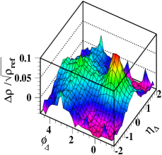
Based on subsequent comparisons of observed data systematics with theory the components (a) and (b) together are interpreted to represent minimum-bias dijets fragevo ; anomalous . Component (c) has been conventionally attributed to elliptic flow 2004 . Component (d) is attributed to projectile-nucleon dissociation. And the 2D exponential is attributed to Bose-Einstein (quantum) correlations and charge-neutral electron pairs from photoconversions (denoted as the BE/electron peak).

V.2 Correlation data models

The fit methods employed here are based on the the non-Fisherian ansatz that data can be represented as the sum of a hypothesis (any competing data parametrization) plus noise. 2D histograms from Ref. anomalous [e.g. Fig. 1 (a) and (c)] were fitted with a data model including several elements applicable to higher RHIC energies and all Au-Au centralities. The 11-parameter model is

$$A(\eta_{\Delta},\phi_{\Delta}) = A_{2D}\exp\left\{-\frac{1}{2}\left[\left(\frac{\phi_{\Delta}}{\sigma_{\phi_{\Delta}}}\right)^{2}+\left(\frac{\eta_{\Delta}}{\sigma_{\eta_{\Delta}}}\right)^{2}\right]\right\}$$

$$+ A_{\rm D}[\cos(\phi_{\Delta}-\pi)+1]/2+A_{0}$$

$$+ A_{\rm Q}2\cos(2\,\phi_{\Delta})+A_{\text{soft}}\,\exp\left\{-\frac{1}{2}\left(\frac{\eta_{\Delta}}{\sigma_{0}}\right)^{2}\right\}$$

$$+ A_{\text{BE}}\exp\left\{-\left[\left(\frac{\phi_{\Delta}}{w_{\phi_{\Delta}}}\right)^{2}+\left(\frac{\eta_{\Delta}}{w_{\eta_{\Delta}}}\right)^{2}\right]^{1/2}\right\}.~{}~{}$$

The definitions of two parameters in that expression ($A_{D}$ and $A_{Q}$) are modified from those in Ref. anomalous .

Figure 1 (right panels) shows typical 2D model fits with Eq. V.2 compared to corresponding data histograms in the left panels. The fit residuals are consistent with bin-wise statistical errors. The general evolution with centrality is monotonic increase of the SS 2D peak and AS dipole amplitudes (dijet structure), substantial increase of the SS peak $\eta_{\Delta}$ width, rapid decrease to zero of the 1D Gaussian on $\eta_{\Delta}$ (soft component) axialci ; ptscale ; anomalous and non-monotonic variation of the quadrupole amplitude davehq .

For the present 1D study we develop simplified versions of the 11-parameter model. In more-central Au-Au collisions the soft component ($A_{\text{soft}}$) falls to zero amplitude, and the BE/electron component ($A_{\text{BE}}$) becomes very narrow anomalous . A 2D model applicable to more-central Au-Au collisions then has 6 parameters

$$A(\eta_{\Delta},\phi_{\Delta}) = A_{2D}\exp\left\{-\frac{1}{2}\left[\left(\frac{\phi_{\Delta}}{\sigma_{\phi_{\Delta}}}\right)^{2}+\left(\frac{\eta_{\Delta}}{\sigma_{\eta_{\Delta}}}\right)^{2}\right]\right\}$$ (15)

$$+ A_{\rm D}[\cos(\phi_{\Delta}-\pi)+1]/2$$

$$+ A_{0}+A_{\rm Q}2\cos(2\,\phi_{\Delta}).$$

The BE/electron component remains significant in a few bins near the origin that can be removed from the fits.

Projection onto 1D azimuth represents large information reduction. The full 2D histogram with $25\times 25$ bins includes 169 independent bins (one independent quadrant due to symmetrization), whereas 1D projections include at most 13 independent bins. A simplified model derived from the 2D data model but applicable to projected 1D azimuth correlations in more-central A-A collisions includes 5 parameters defined to be consistent with the PS introduced in Sec. III

$$A(\phi_{\Delta}) = A_{1D}\exp\left[-\frac{1}{2}\left(\frac{\phi_{\Delta}}{\sigma_{\phi_{\Delta}}}\right)^{2}\,\,\right]$$ (16)

$$- A^{\prime}_{\rm D}2\cos(\phi_{\Delta})$$

$$+ A_{0}+A_{\rm Q}2\cos(2\,\phi_{\Delta}).$$

A further simplification is possible for the most-central (0-5%) bin. The quadrupole amplitude $A_{Q}$ for that centrality is observed to be consistent with zero davehq ; davehq2 . The 1D model then includes only 4 parameters

$$A(\phi_{\Delta}) = A_{1D}\exp\left[-\frac{1}{2}\left(\frac{\phi_{\Delta}}{\sigma_{\phi_{\Delta}}}\right)^{2}\,\,\right]$$ (17)

$$+ A_{0}-A_{\rm D}^{\prime}2\cos(\phi_{\Delta}).$$

Integrating Eqs. (17) and (III) with differential factor $d\phi_{\Delta}=2\pi/N$ gives

$$2\pi P_{0} = A_{1D}\sqrt{2\pi}\sigma_{\phi_{\Delta}}+2\pi A_{0}~{}~{}~{}\text{or}$$ (18)

$$A_{0} = -A_{1D}\sigma_{\phi_{\Delta}}/\sqrt{2\pi}+P_{0}.$$

The 1D data histograms have been adjusted to insure $P_{0}\equiv 0$. A fit to bin-10 data with Eq. 17 determines an offset value $A_{0}=-0.14$. With other fitted parameter values we obtain

$$A_{1D}\sigma_{\phi_{\Delta}}/\sqrt{2\pi} = 0.57\times 0.635/\sqrt{2\pi}=0.144.$$ (19)

The four-parameter 1D model can then be further reduced to a three-parameter model defined by

$$A(\phi_{\Delta}) = A_{1D}\left\{\exp\left[-\frac{1}{2}\left(\frac{\phi_{\Delta}}{\sigma_{\phi_{\Delta}}}\right)^{2}\,\,\right]-\sigma_{\phi_{\Delta}}/\sqrt{2\pi}\right\}$$ (20)

$$- A_{\rm D}^{\prime}2\cos(\phi_{\Delta}),$$

where each of two model components integrates to zero over $2\pi$. We therefore replace Eq. (17) with Eq. (20) referred to below as the “basic Model.”

Since all data histograms are corrected to $P_{0}\equiv 0$ to remove the offset DoF the adjusted 13-bin 1D data histograms have 12 independent DoF. But the bin at $\phi_{\Delta}=0$ is removed from all model fits to exclude the BE/electron component, reducing the effective data DoF to 11.

The AS dipole component is the limiting case of an AS Gaussian peak array (see App. D for details). The r.m.s. peak width ($\sigma\approx\pi/2$) is large enough that only the $m=1$ AS dipole term of the PS representation survives.

We define alternative data models by adding to the basic Model of Eq. (20) successive cosine terms of the form $A_{X}2\cos(m\phi_{\Delta})$, where $X=Q,~{}S,~{}O$ for quadrupole, sextupole and octupole ($m=2,~{}3,~{}4$). We also define independent “FS-only” models as truncated Fourier series with $K$ cosine terms and no other components.

VI Bin-10 0-5% Azimuth correlations

We first apply BI methods to the 1D azimuth projection from 0-5% central 200 GeV Au-Au collisions. We fit the data with the basic Model and obtain the data PS. We determine $\chi^{2}$ and information $I$ for FS-only models vs parameter number $K$. We then evaluate evidence $E$ for several competing models and determine the posterior model probabilities.

VI.1 1D azimuth projection

Figure 2 shows a projection of the 2D data histogram from 0-5% central 200 GeV Au-Au collisions onto 1D $\phi_{\Delta}$ (points). 24 bins are shown but only 13 are unique due to symmetrization about zero and $\pi$. Estimated statistical errors have been multiplied by factor 2 to make them visible (extend outside the points). Errors are a factor $\sqrt{2}$ larger for the bins at 0 and $\pi$ because of symmetrization of the data about those bins. The bin at zero also includes a significant contribution from BE/electrons not included in the models used for this exercise and is therefore excluded from all fits. The bin at $\pi$ includes a small excess due to a tracking-geometry distortion accommodated in some model fits by addition of a “delta function.”

Figure 2: (Color online) 1D projection onto azimuth (points) from the 2D data histogram for 0-5% central 200 GeV Au-Au collisions in Fig. 1 (c). Statistical errors at 0 and $\pi$ are $\sqrt{2}$ larger than the others due to symmetrization of data on the periodic variable. The bin-wise statistical errors 0.0037 have been multiplied by 2 to make them visible outside the data points. The (red) dashed curve is obtained from a fit to the data with the basic Model of Eq. (20). A fit with an FS-only model including four or more terms would appear identical on the scale of this plot. A similar remark applies to corresponding data plots for two other centrality bins.

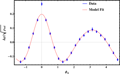
A fit of the basic Model to data is shown by the dashed (red) curve. The fitted model parameters are $A_{1D}=0.57\pm 0.007$, $\sigma_{\phi_{\Delta}}=0.635\pm 0.007$ and $A^{\prime}_{D}=0.115\pm 0.002$ with $\chi^{2}=12.5$ for $11-3=8$ fit DoF.

VI.2 Data power spectrum

Figure 3 shows the PS (points and blue solid curve) as a Fourier transform of the data autocorrelation in Fig. 2 using Eq. (III). The general structure includes a signal component at smaller wave number $m\leq 4$ and a flat (on average) white-noise spectrum at larger wave number corresponding to the r.m.s. statistical error in the data histogram. The noise-spectrum mean is about 0.001 (dotted line).

Figure 3: (Color online) Power spectrum values $P_{m}$ (points) derived from the data in Fig. 2 via Eq. (III). The (red) dashed curve is the Gaussian PS described by Eq. (21) with width and amplitude corresponding to the fitted Gaussian in Fig. 2. Interval $m\geq 5$ is consistent with a “white-noise” power spectrum (dotted line) representing the statistical noise in Fig. 2.

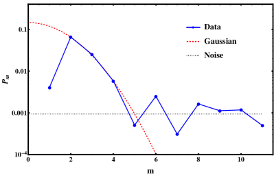
To aid interpretation of the data PS we include the predicted PS for a 1D Gaussian (red dashed curve) with amplitude and width derived from the basic-Model fit in Fig. 2. The PS amplitudes for a unit-amplitude periodic Gaussian peak array on $\phi_{\Delta}$ are given by (App. D)

$$2P_{m}(\sigma_{\phi_{\Delta}}) = \sqrt{2/\pi}\,\sigma_{\phi_{\Delta}}\exp\left(-m^{2}\sigma_{\phi_{\Delta}}^{2}/2\right).$$ (21)

As the Gaussian peak width $\sigma_{\phi_{\Delta}}$ increases the number of significant signal terms in the PS decreases. The Gaussian PS coincides with the data PS for $m\in[2,5]$, and the data PS for $m\geq 5$ is consistent with statistical noise. The data PS element for $m=1$ includes a negative contribution $-A^{\prime}_{D}=-0.115$ from the AS peak (dipole).

We can assess the quality of the basic-Model data description by determining the PS of the residuals, not of (data $-$ Model) but of (data $-$ Gaussian) only. The PS of the residuals should be equal to the PS difference in Fig. 3 according to the linearity of Eq. (III).

Figure 4: (Color online) The PS for residuals in the form (data $-$ Gaussian) from Fig. 2 consistent with the white-noise part of the PS in Fig. 3, with mean approximately 0.001. The negative PS value for $m=1$ (not shown) corresponds to the AS dipole amplitude $-A^{\prime}_{D}$ from the basic-Model fit in Fig. 2.

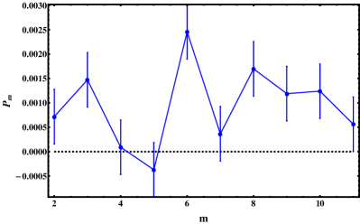
Figure 4 shows the PS for (data $-$ Gaussian) referring to the fitted Gaussian in Fig. 2. The PS values for $m>1$ are consistent with the white-noise spectrum. The value for $m=1$ (not shown) is consistent with the fitted dipole amplitude. From this PS study we have a first indication that the $K=3$ basic Model is sufficient to describe the bin-10 1D azimuth projection.

VI.3 Bayesian model fits with Fourier series

We next apply BI methods to FS-only models of the data histogram in Fig. 2 to establish a BI reference. In this application the number of parameters $K$ represents the largest value of FS index $k$ for a given FS-only model. Varying $K$ represents different FS data models. We obtain the $\chi^{2}$ and information $I$ for each FS-only model.

Figure 5: (Color online) $\chi^{2}$ (upper solid curve and points) and information $2I$ (dashed curve and points with uncertainty band) vs number of parameters $K$ for Fourier-series (FS-only) models. The sum (log Evidence, $-2LE$, dotted curve) is also included. The lower solid curve is $\chi^{2}$ values for fits to residuals (data $-$ basic Model) from Fig. 2 consistent with the trend $11-K$ expected for no signal (noise only) in the data.

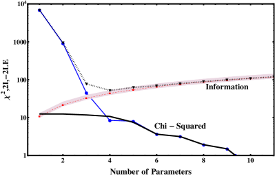
Figure 5 shows the basic elements of BI model fits. The upper (blue) solid curve and points represent the log likelihood (LL) in the form $-2LL$ or $\chi^{2}$. The (red) dashed curve shows information $2I$ representing the parameter cost (Occam penalty, Sec. II.6). The (black) dotted curve represents the sum $-2LE$ (negative log evidence). The minimum for $-2LE$ (and maximum for evidence $E$) occurs at $K=4$ indicating the FS-only model preferred by the data. That result is consistent with Fig. 3 indicating a $K=4$ FS-only model should exhaust the PS signal.

The $\chi^{2}$ trend indicates that the FS model components are ideally ordered on index $k\in[1,K]$ for the signal in these specific data, and is similar to the idealized trend suggested in Fig. 5.1 of Ref. bayes2 . The largest decreases occur for the smallest index values. The interval with larger (negative) slope at smaller $K$ corresponds to accommodation of the data signal with increasing $K$. The interval with smaller slope at larger $K$ indicates that additional Fourier terms only accommodate statistical noise. The overall $\chi^{2}$ trend then matches the power-spectrum trend in Fig. 3. $\chi^{2}$ must go to zero when $K=$ the number of data DoF (11 in this case). The lower solid curve represents the $\chi^{2}$ for fits to the residuals (data $-$ basic Model) from Fig. 2 (no signal present). The $\chi^{2}$ values are then consistent with the fit DoF $\approx 11-K$.

VI.4 Bayesian model comparisons

We next extend BI methods to several data models with different combinations of elements and parameters compared to the previous FS-only exercise. We first compare $\chi^{2}$ alone, simulating a conventional model-fit exercise, then extend to comparisons of evidence $E(D^{*}|H)$.

Figure 6: (Color online) $\chi^{2}$ values vs number of parameters $K$ for several data models. The general trend is monotonic decrease with increasing number of model parameters, responding only to statistical noise with $\chi^{2}\approx 11-K$ for $K>4$.

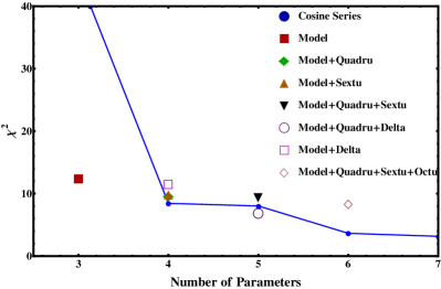
Figure 6 shows $\chi^{2}$ values for various model fits to data. The FS-only description (blue points and line) achieves a substantial decrease for $K=4$ but no significant improvement with additional terms. The basic Model with three parameters (red solid square) has $\chi^{2}\approx 12.5$, somewhat in excess of the number of fit DoF $=8$. Addition of more cosines (quadrupole, sextupole, octupole) to the basic Model keeps pace with the FS noise trend with its reduced slope. In this conventional context the extra cosines seem to be required for competitive data description because they reduce the fitted $\chi^{2}$, but at what cost?

The basic Model + quadrupole + sextupole + octupole with $K=6$ (open diamond) has the same $\chi^{2}$ as the $K=4$ FS-only model. As explained below in connection with Table 1 the additional cosine terms effectively displace the Gaussian part of the basic Model. The composite model then functions as a FS-only model with $K=4$, but with increased cost in the Occam penalty.

Figure 7: (Color online) Negative log evidence $-2LE$ vs number of parameters $K$ for several models. The basic Model (solid square) is strongly favored over all others (lowest $-LE$). The hatched band indicates the common uncertainty of priors assigned to cosine terms in all models. FS-only models for all $K$ (solid dots and line) are strongly rejected by the evidence.

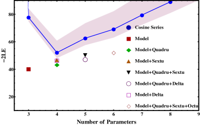
Figure 7 shows negative log evidence $-2LE=\chi^{2}+2I$ for several models. Adding an Occam penalty in the form of information $I$ gained by each model reveals a different picture. The basic Model with $K=3$ has substantially smaller -2LE (larger evidence $E$) than other models where the cost of extra parameters is not justified by a compensating reduction in $\chi^{2}$. The hatched band reflects the estimated uncertainty in $I$ (for the FS-only model) arising from the estimated priors.

Given that $\chi^{2}$ values for various models are similar ($\approx 11-K$) the large differences in $-LE$ among models must be dominated by information $I$ which depends on the covariance matrix and prior PDFs. It might be suggested that such differences arise mainly from the assignment of prior probabilities, but that is not the case. We apply the same prior to a given parameter or parameter class consistently across all models, so that uncertainties in I are strongly correlated across competing models and largely cancel when odds ratios are taken (see Sec. IX.3).

The $LE$ trend vs $K$ for FS-only models arises from $2I\approx 10K$, whereas the $LE$ trend for the basic Model plus additional cosine terms corresponds to $2I\approx 5K$. The difference in $I/K$ of 2.5 corresponds to a factor $\exp(2.5)\approx 12$ difference in parameter errors for the two models. Parameter errors for FS-only models are $O(0.001)$ whereas errors for the basic Model plus cosine terms are $O(0.01)$, accounting for the factor 10-15 difference. As discussed in Sec. X.2 the large Occam penalty for FS-only models is mainly owing to smaller covariance-matrix elements (parameter errors).

Figure 8: (Color online) Normalized $p(H_{l}|D^{*})$ from Eq. (22) for several models indexed by $l$. As in Fig. 7 the basic Model (solid square) is strongly favored over all other models while FS-only models for all $K$ are strongly rejected.

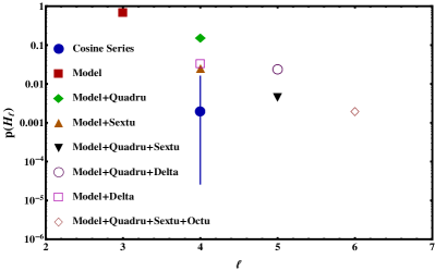
Figure 8 shows the plausibility (relative evidence) for each competing model in the form

$$p(H_{l}|D^{*}) = \frac{E(D^{*}|H_{l})p(H_{l})}{\sum_{l}E(D^{*}|H_{l})p(H_{l})}$$ (22)

that reveals the full selectivity of the BI method. For this exercise we assume that model prior probabilities $p(H_{l})$ are all equal (and therefore irrelevant). However, implicit $p(H_{l})$ assumptions do play a role in RHIC/LHC data modeling and physics interpretations.

The most plausible models are the basic Model (80%) and basic Model + quadrupole (15%). Large Occam penalties reduce competing additional multipole elements to a few percent or less. The model including an octupole (open diamond) leads to major fit instabilities and is rejected. With plausibilities of less than 1% FS-only models are also rejected. In terms of odds the basic Model is preferred over Model + quadrupole by $4.6\pm 0.7$:1, over Model + sextupole by $28.0\pm 4.8$:1 and over all FS-only models by $360\pm 42$:1.

As noted in Section II-E Bayesian comparisons among models are effected by taking ratios of evidences (odds ratios). Comparisons are visualized efficiently by corresponding differences on a log-evidence scale (Bayes factors) as in Fig. 7 and subsequent equivalent figures. Isolated absolute numbers are not relevant to our method.

VI.5 Model-fit results for bin 10

Table 1 summarizes the best-fit model-parameter values $\tilde{w}$ obtained from model fits (minimum $\chi^{2}$) emphasizing the basic Model (column 2) and successive additions of quadrupole, sextupole and octupole components, as well as a delta function at $\pi$ to accommodate a data artifact. The parameters are as defined in Sec. V.2. Also shown are $\chi^{2}$ and the BI parameters $2I$ and $-2LE$.

Table 1: Bin-10 model parameters (minimum $\chi^{2}$) for several fit models: (a) basic Model, (b) basic Model plus quadrupole term $A_{Q}$, (c) previous plus sextupole term $A_{S}$, (d) previous plus octupole term $A_{O}$, (e) basic Model plus delta function at $\pi$. The fit parameters are as defined in Sec. V.2.

parameter	basic Model	+ $A_{\text{Q}}$	+ $A_{\text{S}}$	+ $A_{\text{O}}$	$+\delta$
$A_{1D}$	0.57$\pm 0.007$	0.73$\pm 0.09$	0.84	0.34	0.57
$\sigma_{\phi_{\Delta}}$	0.64$\pm 0.007$	0.69$\pm 0.02$	0.71	0.09	0.63
$A^{\prime}_{D}$	0.12$\pm 0.002$	0.15$\pm 0.02$	0.18	-0.003	0.115
$A_{Q}$	–	-0.014$\pm 0.007$	-0.025	0.064	–
$A_{S}$	–	–	0.005	0.024	–
$A_{O}$	–	–	–	0.005	–
$A_{\delta}$	–	–	–	–	0.005
$\chi^{2}$	12.5	9.7	10	9	11
$2I$	28	34	38	44	36
$-2LE$	40.5	42.5	48	53	47

Results for the basic Model are in good agreement with the published values from 2D model fits anomalous . For this centrality the best-fit 2D parameters from the model of Eq. (V.2) are $A_{2D}=0.65\pm 0.04$, $\sigma_{\phi_{\Delta}}=0.63\pm 0.015$, $A_{0}=-0.14\pm 0.014$ (consistent with the Gaussian integral), $A_{D}=0.224\pm 0.002$ ($\approx 2A^{\prime}_{D}$), $A_{Q}=0.001\pm 0.008$ with $\chi^{2}$ / DoF = 2.6. Note that $A_{1D}$ must be less than $A_{2D}$ because of the curvature on $\eta_{\Delta}$ of the SS 2D peak. The $\chi^{2}$/DoF = 2.8 of the 2D model fit is substantially higher than that for the 1D fit with the basic Model [12.5 / (11 - 3) = 1.6] because of significant structure on $\eta_{\Delta}$ ($\eta$-modulated dipole) not described by the standard 2D data model of Eq. (V.2).

As cosine terms are added to the basic Model a conflict develops between the explicit Gaussian component and a sum of cosines approximating a competing Gaussian. The large parameter differences for “$+A_{O}$” vs “basic Model” columns are discussed further in Sec. X.3.

The $+\delta$ column refers to the basic Model plus a free amplitude in the bin at $\pi$ (“delta function”). Compared to the basic Model alone there is reduction of $\chi^{2}$ by 1.5 but increase of information $2I$ by 8 leading to overall increase of negative log evidence $-2LE$ by 6.5. The additional model DoF is rejected by $\exp(3.25)\rightarrow$ 25:1.

VII bin-8 9-18% Azimuth correlations

In this second of three examples the statistical errors of the wider centrality bin are reduced by factor $\sqrt{2}$ compared to the 0-5% centrality bin. The BE/electron peak is still narrow enough to remain within the single bin at zero. The quadrupole component is significant and positive, shifting the plausibility order of competing models.

VII.1 1D azimuth projection

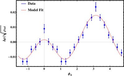
Figure 9 shows a projection of the 2D data histogram from 9-18% central 200 GeV Au-Au collisions onto 1D $\phi_{\Delta}$ (points). As for the previous centrality the bin at zero also includes a significant contribution from BE/electrons not included in the data models and is therefore excluded from the fits. The typical data r.m.s. statistical error is 0.0026, not visible outside the points on this scale.

Figure 9: (Color online) 1D projection onto azimuth (points) from the 2D data histogram for 9 - 18% central 200 GeV Au-Au collisions. The (red) dashed curve is a fit to the data with the basic Model of Eq. (20) plus independent quadrupole component $A_{Q}2\cos(2\phi_{\Delta})$. The bin-wise statistical errors are 0.0026, not visible outside the points.

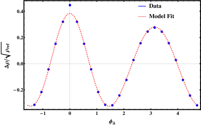
A fit of the basic Model + quadrupole to data is shown by the dashed (red) curve. The fitted model parameters are $A_{1D}=0.926\pm 0.088$, $\sigma_{\phi_{\Delta}}=0.727\pm 0.018$, $A^{\prime}_{D}=0.206\pm 0.022$ and $A_{Q}=0.068\pm 0.006$ with $\chi^{2}=16.5$ for 11 - 4 = 7 fit DoF.

VII.2 Data power spectrum

Figure 10 shows the power spectrum (points and blue solid curve) derived from the data in Fig. 9. As for the 0-5% centrality bin we include the predicted power spectrum (red dashed curve) for a 1D Gaussian (SS peak) with amplitude and width parameters derived from the fit to data in Fig. 9. The data PS is again consistent with statistical noise for $m\geq 5$. The PS element for $m=1$ includes a negative contribution from the AS dipole. The element for $m=2$ includes a significant positive contribution from a quadrupole component not associated with the SS peak davehq .

Figure 10: (Color online) Power spectrum values $P_{m}$ (points) derived from the data in Fig. 9 via Eq. (III). The (red) dashed curve is the Gaussian PS described by Eq. (21) with amplitude and width from the basic Model + quadrupole fitted to data in Fig. 9. The interval $m\geq 5$ is consistent with a “white-noise” power spectrum (dotted line) representing the statistical noise in Fig. 9.

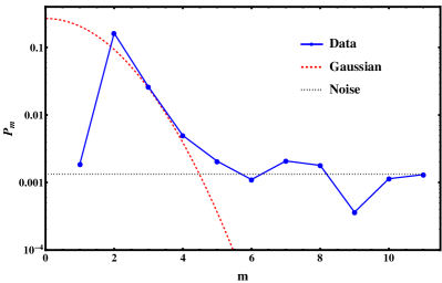
Just as for bin 10 we assess the quality of the basic-Model data description by determining the PS of the residuals of (data $-$ Gaussian) only, where Gaussian is the fitted Gaussian in Fig. 9. The PS for (data $-$ Gaussian) is consistent with a white-noise spectrum with mean value $\approx 0.0013$ for $m>2$. The values for $m=1,$ 2 are consistent with the fitted positive quadrupole and negative dipole amplitudes. The basic Model augmented by quadrupole component $\cos(2\phi_{\Delta})$ fully exhausts the data signal and is therefore a sufficient model.

VII.3 Bayesian model fits with Fourier series

The log-likelihood LL trend in the form $\chi^{2}$ for $K>2$ for FS-only model fits to data from bin 8 (not shown) is similar to that for bin-10 data in Fig. 5. Information $2I$ representing the parameter cost is also similar. The minimum of $-2LE$ occurs at $K=4$, consistent with Fig. 10 where we again find that a $K=4$ FS-only model should completely describe the signal in the bin-8 data. The FS-only model should then be competitive with the $K=4$ basic Model + quadrupole in terms of fit quality and parameter number, two elements of BI evaluation.

VII.4 Bayesian model comparisons

Figure 11 shows $\chi^{2}$ values from conventional data modeling. The FS-only model achieves a substantial reduction for $K=4$ but no significant improvement for additional terms. The basic Model with $K=3$ (solid red square) has a $\chi^{2}$ much elevated from the number of fit DoF = 8 and is rejected on that basis. Addition of a quadrupole component (solid green diamond) brings $\chi^{2}$ down to an acceptable value. Addition of more cosines (sextupole, octupole) to the basic Model + quadrupole tracks the FS-only noise accommodation.

Figure 11: (Color online) $\chi^{2}$ values vs number of parameters $K$ for several data models. The general trend is again monotonic decrease with increasing parameter number.

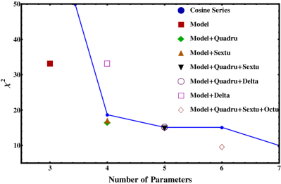
The basic Model + sextupole (solid red triangle) has the same $\chi^{2}$ value as that for basic Model + quadrupole. The Gaussian + dipole + sextupole combination can interact to accommodate the independent quadrupole component in the data, since the octupole component of the Gaussian is only a few sigma above the statistical noise. Interactions among the basic Model Gaussian and additional cosine terms are discussed in Sec. X.3.

Figure 12: (Color online) Negative log Evidence $-2LE$ vs number of parameters $K$ for several models. The basic Model + quadrupole (solid diamond) is strongly favored over others (lowest $-LE$, largest evidence). The basic Model alone (solid square) is strongly rejected by the evidence, as are FS-only models for all $K$ (blue points and line).

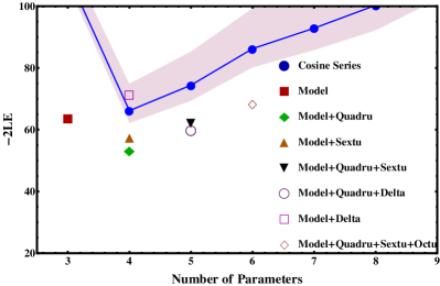
Figure 12 shows negative log evidence $-2LE$ for various models. The basic Model + quadrupole (solid green diamond) corresponding to $K=4$ model DoF has substantially smaller -2LE (larger evidence $E$) than other model combinations. It is clearly preferred over the basic Model alone by $\exp(5)\rightarrow 187\pm 30$:1 odds. For other models the cost of extra parameters is not justified by reductions in $\chi^{2}$. The quadrupole model component is preferred over a sextupole by $\exp(2)\rightarrow 8.5\pm 1.4$:1 due to differences in the fit covariance matrix for the two models. All FS-only models are again rejected by large factors.

VIII bin-0 83-94% Azimuth correlations

In this third of three cases, essentially representing $p$-$p$ ($N$-$N$) collisions, we encounter a major challenge for BI analysis from several sources: (a) The SS peak on azimuth contains two contributions that cannot be separated easily by discarding the bin at the origin as they were for bins 8 and 10, (b) the signal amplitude is much smaller relative to statistical noise (15:1) than it was for more-central collisions (200:1), and (c) the SS peak is substantially broader on azimuth.

VIII.1 1D azimuth projection

Figure 13 shows a projection of the 2D data histogram from 83-94% central 200 GeV Au-Au collisions (points). Unlike previous cases the SS peak includes a significant contribution from BE/electrons that is not included in the models (conversion electron pairs do fall mainly within the single bin at the origin). A fit of the basic Model to data is shown by the dashed (red) curve. The fitted model parameters are $A_{1D}=0.073\pm 0.025$, $\sigma_{\phi_{\Delta}}=0.926\pm 0.128$ and $A^{\prime}_{D}=0.022\pm 0.006$ with $\chi^{2}\text{/DoF}=12.0$ for 11 - 3 = 8 fit DoF.

Figure 13: (Color online) 1D projection onto azimuth (points) from the 2D data histogram for 83 - 94% central 200 GeV Au-Au collisions in Fig. 1 (a). The (red) dashed curve is a fit to the data with the basic Model of Eq. (20). The statistical errors are 0.0026.

VIII.2 Data power spectrum

Figure 14 shows the power spectrum (points and blue solid curve) derived from the data in Fig. 13. As for previous centrality bins we include a predicted power spectrum (red dashed curve) for a 1D Gaussian (SS peak) with amplitude and width parameters derived from the basic Model fitted to data in Fig. 13.

Figure 14: (Color online) Power spectrum values $P_{m}$ (points) derived from the data in Fig. 13 via Eq. (III). The (red) dashed curve is the Gaussian PS described by Eq. (21) with Gaussian width and amplitude corresponding to the basic Model fitted to data in Fig. 13. The interval $m>2$ is consistent with a “white-noise” power spectrum (dotted line) representing the statistical noise in Fig. 13.

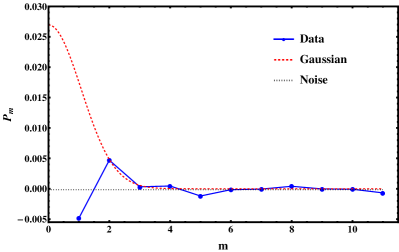
Because the bin-0 SS peak is broader on azimuth (thus narrower on index $m$) and the S/N is much smaller the PS signal is not significant at $m=4$ or even $m=3$. A $K=2$ FS-only model in the form of dipole + quadrupole should be sufficient to displace the basic Model. For bins 10 and 8 FS-only models are clearly excluded in favor of the basic Model, but for bin 0 the $K=3$ basic Model and a $K=2$ FS can both describe the two data DoF. Thus, we expect BI analysis to prefer the FS-only model.

VIII.3 Bayesian model fits with Fourier series

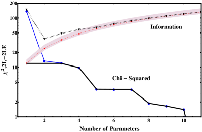
Figure 15 shows the FS-only $\chi^{2}$ trend for bin-0 data (upper solid blue curve and points). As expected, $\chi^{2}$ drops to the noise trend (lower solid curve) by $K=2$. Additional terms accommodate statistical noise. Information $2I$ follows the expected monotonic increase $\approx 10K$. Negative log evidence $-2LE$ has a minimum for $K=2$. Thus, an FS-only model with $K=2$ is preferred by the data, as expected from the PS in Fig. 14.

Figure 15: (Color online) $\chi^{2}$ (upper solid curve and points) and information $2I$ (dashed curve and points) vs number of parameters $K$ for FS-only models. The sum $-2LE$ (dotted curve and points) is also included. The $\chi^{2}$ trend for basic-Model fit residuals (lower solid curve) is approximately consistent with the expected noise trend $11-K$.

VIII.4 Bayesian model comparisons

Figure 16 shows $\chi^{2}$ trends for several competing models applied to the bin-0 data in Fig. 13. The $K=3$ basic Model and FS-only model describe the data equally well, and we expect the simpler $K=2$ FS-only model to be preferred when an Occam penalty is included. For these bin-0 data the addition of a “delta” component at $\pi$ (open square) leads to substantial improvement in the fit quality, consistent with Fig. 13.

Figure 16: (Color online) $\chi^{2}$ values vs number of parameters $K$ for several data models. The basic Model (solid square) is equivalent to the FS-only model with $K=3$ (solid dot).

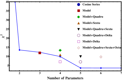
Figure 17 shows the log evidence $-2LE$ trend. That the $K=3$ basic Model (solid red square) is preferred over the $K=2$ FS-only model (lowest blue point) despite the cost of the extra model parameter is a major surprise. The evidence ratio (odds) is $3.3\pm 0.25$:1 $\approx\exp(1.25)$. That result prompted a detailed study reported in Sec. X.2 on how information $I$ is related to model priors and data, with supporting material provided in App. A.

Figure 17: (Color online) Negative log Evidence $-2LE$ vs number of parameters $K$ for several models. The $K=3$ basic Model (solid square) is favored over all others (lowest $-LE$, largest evidence), especially over the $K=2$ FS-only model expected to prevail for this centrality (lowest solid dot).

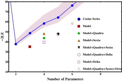
The ability in this case to discriminate between the basic Model and FS models, despite 1D data with low S/N ratio, is a significant achievement for BI analysis. The correctness of the basic-Model preference is confirmed by analysis of 2D data histograms. From the 2D analysis of Ref. anomalous we learn that the SS 2D peak is necessary for all centralities. In contrast, a 1D FS-only model would fail dramatically for any 2D data, but that is not apparent from 1D projections alone.

IX Systematic uncertainties

Bayesian Inference methods provide a powerful system for discriminating among competing complex data models with a consistent set of evaluation rules. Close examination of method details and evaluation of uncertainties is required to insure confidence in the results.

IX.1 Uncertainties for data histograms

For 2D histograms from Ref. anomalous the angular acceptance was divided into 25 bins on the $\eta_{\Delta}$ axis and 25 bins on $\phi_{\Delta}$, a trade off between statistical error magnitude and angular resolution. The histograms are by construction symmetric about $\eta_{\Delta}=0$ and $\phi_{\Delta}=0,\pi$. The 25 bins on $\phi_{\Delta}$ actually span $2\pi+\pi/12$ to insure centering of major peaks on azimuth bin centers. 2D binwise statistical errors are $\pm 0.004$ for 200 GeV data near $|\eta_{\Delta}|=0$. Because of the $\eta_{\Delta}$ dependence of the pair acceptance statistical errors increase with $|\eta_{\Delta}|$ as $\sqrt{\Delta\eta/(\Delta\eta-|\eta_{\Delta}|)}$ with $\eta$ acceptance $\Delta\eta=2$. Errors are uniform on $\phi_{\Delta}$ except that errors are larger by factor $\sqrt{2}$ for angle bins with $\phi_{\Delta}=0$ and $\pm\pi$ because of reflection symmetries.

Statistical errors are approximately independent of centrality for the per-particle statistical measure $\Delta\rho/\sqrt{\rho_{\text{ref}}}$ over nine 10% centrality bins (0-8). An additional factor $\sqrt{2}$ increase applies to the two most-central centrality bins (9, 10) which split the top 10% of the total cross section. After projection onto 1D azimuth for this study the centrality bin 10 errors are about 0.0037 except for the azimuth bins at 0 and $\pi$. Errors for the other centrality bins (0, 8) are a factor $1/\sqrt{2}$ less or 0.0026. $\chi^{2}$ values for optimized models in this study determined with those statistical errors are generally consistent with the number of fit DoF = data DoF $-$ K (number of model parameters), as demonstrated in Fig. 5. Thus, the statistical and systematic uncertainties for data histograms used in this study are both small and well understood.

IX.2 Uncertainties for information estimation

Information uncertainty is largely related to the choice of prior PDFs for various model parameters and the fitted-parameter uncertainties. We repeat the information definition in Eq. (7)

$$I(D^{*}|H) = -\ln\left[\sqrt{(2\pi)^{K}\det C_{K}}~{}p(\tilde{w}|H)\right],$$ (23)

the natural log of prior volume $V_{w}(H)$ over posterior volume $V_{w}(D^{*}|H)$ in the model parameter space. The covariance matrix $C_{K}$ for a $K$-parameter model is obtained from the Hessian describing the curvatures of the likelihood function near its maximum. The likelihood function is in turn determined by model $H$ in combination with specific data $D^{*}$. If the model and prior are defined and data specified the posterior volume is also well defined.

Assuming translation invariance within a parameter-space volume where the likelihood is significantly nonzero the prior PDF for parameter $w_{k}$ is taken to be uniform across a bounded interval $\Delta_{k}$ into which the corresponding fitted parameter value should almost certainly fall. The prior volume for $K$ parameters is then

$$1/p(\tilde{w}|H) = \prod_{k=1}^{K}\Delta_{k}\equiv V_{w}(H).$$ (24)

In principle, a prior is defined before data $D^{*}$ are obtained and thus should not depend on specific data. However, it is fair to invoke general knowledge ($Q$) about the typical amplitudes of structures in such data. We know from experience that typical structure amplitudes (e.g. peak-to-peak excursions) are generally $<O(1)$. That applies for example to the Gaussian amplitude in the basic Model, and to the Gaussian width based on the definition of the SS peak, implying that $\Delta_{k}\approx 1$ in those cases.

What matters more than absolute estimates of $\Delta_{k}$ is the relations among different models and model parameters. If prior-interval estimates are excessive for a particular model it may be unduly penalized. Given the above assignment for a Gaussian amplitude, what is a fair assignment for cosine coefficients? To that end we examine Eq. (III). The autocorrelation to be modeled on the left receives contributions at the origin from several FS components $P_{m}$ including factors 2. Thus, it is reasonable to assume that cosine coefficients and uncertainties may be substantially smaller on average than the Gaussian amplitude and uncertainty. For all cosine components we assign $\Delta_{k}=1/3$ and indicate prior-related uncertainties by including $\Delta_{k}=1$ and $\Delta_{k}=1/5$ as limiting cases for cosines (e.g. curve $I$ and hatched band in Fig. 5).

If we assume equal prior intervals $\Delta_{k}$ and equal variances $\sigma_{k}^{2}$ for $K$ model parameters and negligible covariances among parameters information $I$ simplifies to

$$I \approx K\left\langle\ln\left[\frac{\Delta_{k}}{\sqrt{2\pi}\sigma_{k}}\right]\right\rangle+\text{constant}.$$ (25)

In fits with FS-only models we observe $\sigma_{k}\approx O(0.0007)$. Given $\Delta_{k}\approx 1$ we have $\ln(\Delta_{k}/\sqrt{2\pi}\sigma_{k})\approx 6$, while if we reduce to $\Delta_{k}\rightarrow 1/3$ (assumed for all cosine terms) $\ln(\Delta_{k}/\sqrt{2\pi}\sigma_{k})\approx 5$. If we further reduce $\Delta_{k}\rightarrow 1/5$ with $\ln(\Delta_{k}/\sqrt{2\pi}\sigma_{k})\approx 4.7$ the fitted parameter values in some cases contradict the prior, implying that the chosen prior interval is too small. We can then state that for all FS-only models $I/K=5.3\pm 0.6$. For the basic model with added cosines the parameter uncertainties are more typically $\sigma_{k}\approx O(0.01)$. In that case we obtain $I/K=2.6\pm 0.5$. Those results imply that addition of a model parameter is justified ($-2LE=\chi^{2}+2I$ is significantly reduced) if the resulting decrease in $\chi^{2}$ is significantly greater than $2I/K\approx 10$ for FS-only models and $\approx 5$ for the basic Model plus optional cosines.

IX.3 Uncertainties for odds ratios

As noted in Sec. II.5 odds ratios can be used to state quantitatively the BI relation between two models in the form of a probability ratio $p(D^{*}|H_{1})/p(D^{*}|H_{2})\rightarrow E(D^{*}|H_{1})/E(D^{*}|H_{2})$, where equality to the second ratio assumes equal model priors $p(H)$ for the two cases. In terms of log evidence $LE$ the Bayes Factor is $B_{12}=\ln[E(D^{*}|H_{1})/E(D^{*}|H_{2})]$, and the odds is then $\exp(B_{12})$.

The uncertainty (error) in an odds ratio is determined by the uncertainties in the compared evidences in turn dominated by uncertainties in the covariance matrix/Hessian and the prior PDFs. Uncertainties for the Hessian matrix are discussed in App. B and serve as the sole basis for the odds errors stated in the text.

Uncertainties for the prior PDFs are discussed in the previous subsection. The priors for SS Gaussian amplitude and width are set to the minimum values consistent with experience, disfavoring the basic Model a priori and implying that any odds favoring the basic Model is a lower limit. A common uncertainty of a factor 2 either way is assumed for a cosine coefficient in any model. Because an odds estimate is a probability ratio systematic errors correlated between numerator and denominator cancel in first order, whereas uncorrelated random errors should combine quadratically. That property can be seen as an advantage for odds as a basis for model comparisons and minimizes the uncertainty contribution from cosine elements common to two compared models.

If models with different $K$ values (parameter number) are compared the unpaired systematic error is not canceled. For instance, the odds between the basic Model ($K=3$) vs FS-only model ($K=4$) for bin 10 includes a linear dependence on the FS-only prior uncertainty for one additional cosine term. However, the comparison of basic Model plus quadrupole vs FS-only model for bin 8 (both $K=4$) eliminates that uncertainty contribution.

X Discussion

We consider several issues that have arisen in application of BI methods to azimuth-correlation data models, including surprising performance of the 1D basic Model in peripheral collisions, consistent strong preference for the basic Model by BI analysis, competition between Gaussian and cosine terms in data models, and implications from this study for two theoretical narratives.

X.1 Comparing bin 10 and bin 0

The data structure for centrality bin 10 in Fig. 2 could be modeled as (a) two peaks at 0 and $\pi$, (b) as a Fourier series only, or (c) as a combination of such elements. The two peaks described by the basic Model are expected in a HEP/jets narrative describing high-energy nuclear collisions. FS models are expected in a QGP/flow narrative and are capable of describing any structure on periodic azimuth. Competition among data models thus reflects competition between theoretical narratives.

In Fig. 3 we learn that all information in the data PS is confined to $m\in[1,4]$. Higher terms in an FS model describe only statistical noise. Comparing a PS Gaussian model with the data PS we find that four points are predicted by a Gaussian fitted to data, and one point corresponds to the fitted dipole within the basic Model. The $K=3$ basic Model fully represents the data signal as demonstrated in Fig. 4, but so does a $K=4$ FS-only model. Intermediate combinations of Gaussian + cosines also describe the data well. Models with more parameters continue to reduce $\chi^{2}$ as in Fig. 6, and might be preferred on that basis.

However, when an Occam penalty is introduced in the form of information $I$ dramatic differences among models appear, as in Figs. 7 and 8. In the latter figure the basic-Model probability is $p(H_{l})\approx 80$%, the next highest being basic Model + quadrupole with $p(H_{l})\approx 15$%. Adding more cosine components may reduce $\chi^{2}$, but not to an extent that compensates large Occam penalties (increase in $I$). The additions are essentially “fitting the noise” and are strongly rejected by BI analysis.

A different situation emerges for Bin 0. In Fig. 14 the data signal is confined to $m\in[1.2]$ for two reasons: (a) The S/N ratio is reduced by a factor 13 and (b) the SS peak azimuth width is increased by 30% so the conjugate PS signal peak width is reduced by that factor. Consequently the “bandwidth” of the data PS signal is reduced from $m\in[1,4]$ to $m\in[1,2]$. A $K=2$ FS-only model with two parameters should then be strongly preferred by BI analysis over the $K=3$ basic Model, given equivalent priors for the two models.

However, that is not what we find in Fig. 17. The basic Model maintains a significant advantage over a $K=2$ FS-only model, the odds ratio being $\approx\exp(1.25)=3.5:1$ in favor of the basic Model, even with one more parameter. That surprising result led to the detailed comparisons in the next subsection and the study in App. A.

The 1D projection is not the only information we have about the source of these data. The unprojected 2D histogram in Fig. 1 (a) clearly indicates that a SS 2D peak model is required by bin-0 data, and a 2D FS-only model would be rejected by a large factor anomalous ; multipoles . The 2D observations contribute a larger Bayesian context ($Q$) applicable to this 1D BI study. The FS-only model is ruled out for all 2D histograms as shown in previous studies multipoles .

X.2 Why BI analysis favors the basic Model

The basic Model alone (for near-central collisions) or the basic Model plus quadrupole (for noncentral collisions) is strongly preferred by BI analysis over FS-only models, even for the most-peripheral collisions where the 1D data include only two significant DoF. The choice of priors is not the reason; priors are applied consistently for each parameter type within any model. The large difference in evidence values is dominated by differences in the fit covariance matrix. The r.m.s. parameter errors for FS models are consistently 10-15 times smaller than for the basic Model. Evidence differences correspond to differences in model predictivity, as illustrated in the following comparison and App. A.

Figure 18 shows sketches of joint data-parameter spaces for an FS-only model (left) and the basic Model (right) corresponding to bin-10 data. The parameter errors for the FS-only model are typically $\sigma_{k}\approx 0.0007$. The parameter errors for the basic Model in Table 1 are 0.007 for SS peak amplitude and width and 0.002 for dipole amplitude, but with added cosine terms the errors increase to $\approx 0.01$. The data errors for bin 10 are $\sigma_{D}\approx 0.0037$. In terms of angles $\theta_{kn}$ defined in Eq. (28) $\tan(\theta_{kn})\approx$ 1/3 for the basic Model (20°) and 5 for the FS-only model (80°). The errors and $\tan(\theta_{kn})$ are represented by the dashed rectangles and the angles of the diagonals (solid lines) in the two panels, as in Fig. 19.

Figure 18: Joint parameter-data space for two data models. These panels are zoomed out from the scale of Fig. 19 to reveal the PDFs distributed over the entire parameter and data spaces. Given prior intervals $\Delta_{k}$ the model angles $\theta_{kn}$ determine the magnitudes of the predicted data intervals $\Delta_{n}$, the predicted data volume $V_{D}(H)$, and therefore the evidence $E(D^{*}|H)$. The $\theta_{kn}$, and hence the Jacobian of a model function, largely determine the predictivity of a model. For these two models the typical $\tan(\theta_{kn})$ differ by factor 12.

In Fig. 18 the prior PDFs are represented by the vertical dash-dotted lines in each panel and the arrows labeled $\Delta_{k}$. For all cosine amplitudes the prior is $\Delta_{k}\approx 1/3$. For the SS peak amplitude and width the priors are $\Delta_{k}\approx 1$. We can estimate the evidences or predicted data volumes based on the argument in App. A where the relation between data-space volume and parameter-space volume is determined by angle factors $\tan(\theta_{kn})$. For the basic Model (right panel) even the larger priors ($\Delta_{k}\approx 1$) are mapped to smaller data intervals ($\Delta_{n}\approx 1/3$), whereas for FS-only models (left panel) smaller priors ($\Delta_{k}\approx 1/3$) are mapped to larger data intervals ($\Delta_{n}\approx 5/3$). The result is much smaller predicted data volumes $V_{D}(H)$ for the basic Model, and consequently much higher evidence and plausibility compared to FS-only models.

The same argument applies to changes in evidence or information with increasing parameter number (e.g. added cosine terms). From Eq. (A.4) (assuming comparable $\chi^{2}$ values for competing models)

$$I = \sum_{k=1}^{K}\ln\left[\frac{\Delta_{k}}{\sqrt{2\pi}\sigma_{k}}\right]+\text{constant}.$$ (26)

With $\Delta_{k}\approx 1/3$ for all cosine terms, $\sigma_{k}\approx 0.0007$ for FS-only models and $\approx 0.01$ for basic Model + cosines the typical increment per cosine term is $I/K\approx 5$ for FS-only models and 2.5 for basic Model + cosines, e.g. consistent with Fig. 7. Thus, evidence and information trends are determined mainly by the relative parameter errors reflecting the Jacobians and model algebra.

The fitted-parameter errors reflect the algebraic structure of the model, as discussed in App. A. Because a Fourier series is orthogonal each coefficient is determined independently. Since the Fourier model elements individually do not resemble the data there is required a very ”fragile” assembly of terms that easily overfits the data (treats noise as signal). Only a small range of FS-only parameter values can reproduce a given data set, and the parameter variances are consequently very small.

In contrast, the basis Model includes a Gaussian (motivated by the data structure) with nonlinear parameter $\sigma_{\phi}$ that covaries with other parameters. Thus, larger ranges of basic-Model parameters can reproduce the data adequately, and the parameter variances are correspondingly larger. The basic Model is more ”robust” because on average the model elements individually look more like isolated data components. If both models give the same chi-squared fit the basic Model is preferred by BI analysis because on average it is far more likely to describe the data accurately (a larger fraction of the prior-delimited parameter space provides an acceptable description for the given data).

We conclude that the key issue for Bayesian model comparisons is model predictivity. The basic Model is highly predictive (therefore falsifiable), describing two peaks (fixed at 0 and $\pi$), with one peak as wide as possible and the other somewhat narrower. Two peak amplitudes and a width are the only parameters. The basic Model is consistent with the HEP/jets narrative but was inferred from data without any theory assumptions. In contrast, FS-only models can describe any structure on azimuth, have no predictivity (are not falsifiable) and are therefore strongly rejected by BI analysis. Model predictivity [smallness of predicted data volume $V_{D}(H)$] is determined largely by the algebraic structure of the data model (Jacobian) as revealed by fitted-parameter errors compared to data errors via the $\tan(\theta_{kn})$ elements.

X.3 Competition: extra cosine terms vs SS Gaussian

The bin-10 results in Table 1 can be used to examine the consequences of adding one or more cosine terms to the basic Model when there is no corresponding data signal. The $\chi^{2}$ is reduced in general, suggesting an improved data description. However, in some cases the model parameters undergo large changes seeming to indicate that model parameters are very uncertain. To understand the apparent contradiction we consider the bin-10 “worst case” model (basic Model + quadrupole + sextupole + octupole) appearing in the next-to-last column of Table 1.

The model difference (“$+A_{O}$” $-$ basic Model) for each cosine coefficient is $\Delta A^{\prime}_{D}=0.115$, $\Delta A_{Q}=0.064$, $\Delta A_{S}=0.024$ and $\Delta A_{O}=0.005$ for $m\in[1,4]$. The differences correspond to the predicted Gaussian PS values in Fig. 3 (red dashed curve). In effect, changes in the cosine coefficients of the FS-only model are equivalent to the fitted Gaussian already describing the data signal correctly in the basic Model. The SS Gaussian required by the data is effectively excluded from the data model by the added cosine terms, reduced to a minor role sextupole .

The bin-10 result reveals a competition between the basic Model and a truncated FS to describe signal + noise. The competing truncated FS offers more flexibility in accommodating noise compared to the monolithic Gaussian. The FS may “win” in terms of $\chi^{2}$, but a well-chosen model element (Gaussian) describes only the signal and excludes the noise. Referring to Fig. 6 the $K=6$ (“+ $A_{O}$”) model (open diamond) has the same $\chi^{2}$ value as the $K=4$ FS-only model (solid point) because the former is effectively a $K=4$ FS. The Gaussian, with two parameters, has been excluded from the fit model owing to noise competition, but its two parameters still contribute to the Occam penalty. BI analysis then rejects the unnecessary cosine terms in favor of the basic Model.

X.4 Evidence extending beyond single histograms

A model may describe data from some A-A centralities well but others poorly. Nevertheless, the model may be retained by convention because of desirable features (such as flow interpretations). Other forms of data selection ($p_{t}$ cuts, 1D projections, ratio measures) present similar issues. In response we propose to extend BI methods beyond single data histograms, combining results into one comprehensive evaluation for competing data models.

The mechanism is suggested by the nature of Bayesian evidence $E$. The evidence is a probability, and by the rules governing probabilities the joint evidence for several cases should be the product of elementary evidences (assuming approximate independence). For instance, the evidence for a model of 200 GeV Au-Au collisions should be the product of evidences for individual centralities. If a model claiming to describe all data components is falsified for one component then it is falsified for all. More generally, a model that provides an adequate description for all cases may be preferred over a model that is favored for some cases but strongly disfavored for others.

That principle extends not only to A-A centralities but to different collision energies, A-B collision systems, spectrum and correlation measures and data cuts. Evidence $E$ as a product measure introduces an “and” condition for data description. A candidate model must address all available data within its parameter space or be rejected.

X.5 Implications for theoretical narratives

As noted in the introduction HEP/jets and QGP/flow narratives currently compete to describe and interpret high-energy nuclear-collision data through choices of data model and emphasis on specific data and measured quantities. The HEP/jets narrative predicts two dijet-related peaks on 1D azimuth, just what the basic Model describes. Almost all 1D azimuth correlation data from the RHIC are described by the basic Model + quadrupole with modest parameter variations. The QGP/flow narrative prefers various forms of the FS-only data model interpreted physically in a flow context, from a single cosine ($v_{2}$, index $k=2$) to several cosines interpreted to include “higher harmonic” flows (index $k\in[1,5]$).

In the present study we apply BI methods to 1D azimuth data models associated with the two narratives. BI analysis strongly favors the basic Model in all cases, combined with an additional quadrupole $\cos(2\phi)$ term except for the most-central data. The FS-only model is strongly rejected in all cases. As discussed in Sec. X.2 and App. A the main reason for BI rejection is lack of predictivity for FS-only models, whereas the basic Model is strongly predictive and therefore falsifiable. The present BI analysis thus seems to support the HEP/jets narrative and reject the QGP/flow narrative per their data models.

It could be argued that application of BI methods to data models represents an arbitrary choice motivated by interest in a specific outcome. However, we are faced with the requirement to evaluate conflicting data models according to some neutral criteria. $\chi^{2}$ minimization always prefers more-complex data models that may reveal little about data structure and possible physical mechanisms. Flow interpretations are always possible for FS-only models, but such models cannot exclude a dijet interpretation since they are able to describe any data configuration.

Additional criteria are therefore required to test data models. Guidance as to choice is provided by the role of rational inference within the scientific method. It is recognized that physical theories cannot be proven, can only be falsified by data, requiring that candidate theories be predictive. Unpredictive theories are not falsifiable and are therefore rejected as candidates. In a Bayesian context predictivity is measured by information $I$ and evidence $E$ as demonstrated in this study. For a well-tested physical theory $H$ encountering new data $D^{*}$ the information $I\approx 0$, and the predicted data-space volume $V_{D}(H)$ is small. If $D^{*}\notin V_{D}(H)$ the theory is falsified but $D^{*}\in V_{D}(H)$ results in plausibility $p(H|D^{*})\to 1$: dramatically different results

In the present analysis we encounter not competing physical theories but competing data models serving as proxies. BI analysis evaluates data models according to predictivity, i.e. the degree of restriction on allowed data configurations. We conclude that the basic Model with optional quadrupole component is very predictive, corresponding to small information gain from newly-received data and consequent small predicted data-space volume. FS-only models are not predictive, can accommodate any data configuration, and are therefore rejected.

XI Summary and Conclusions

Based on data from the relativistic heavy ion collider (RHIC) and large hadron collider (LHC) claims have been made for formation in high-energy nucleus-nucleus (A-A) collisions of a strongly-coupled quark-gluon plasma (sQGP) with small viscosity – a “perfect liquid.” Such claims are based mainly on measurements of Fourier coefficients $v_{m}$ of cosine terms $\cos(m\phi)$ used to describe two-particle correlations on azimuth $\phi$ and interpreted to represent flows, especially $v_{2}$ representing elliptic flow. In the flow context dijets play a comparatively negligible role in final-state correlation structure.

Modeling azimuth correlations by truncated Fourier series or individual cosine terms is not unique. Other model functions can describe the same data equally well and do suggest alternative physical interpretations, especially substantial contributions from dijet production. In effect, two physics narratives compete to describe and interpret the same data. In one narrative collision dynamics is dominated by dijet production. In the other narrative collision dynamics is dominated by a dense, flowing QCD medium. Opposing narratives appear to be supported by their respective data models. To break the deadlock a method is required to evaluate model functions according to neutral criteria and identify a preferred model.

In this study we introduce Bayesian Inference (BI) to evaluate competing model functions. BI analysis relies on a combination of the usual $\chi^{2}$ goodness-of-fit parameter and information $I$ derived from the fit covariance matrix. $I$ quantifies changes in the data model arising from acquisition of new data and represents an Occam penalty for excessive model complexity. Combination $\chi^{2}/2+I$ leads to evidence parameter $E$ that determines the plausibility of each model when confronted with new data values. The goal is to rank data models according to BI criteria without resorting to a priori physics assumptions.

We apply several representative model functions to angular correlation data and evaluate the model performance with BI methods. The data are published 2D angular correlations from three centrality classes of 200 GeV Au-Au collisions on $(\eta,\phi)$. 2D histograms are projected onto periodic azimuth $\phi$ by integration over pseudorapidity $\eta$. The three collision centralities include the centrality extremes (most central and most peripheral) and an intermediate centrality that requires a separate azimuth-quadrupole model element in the data model.

Model functions include (a) a “basic Model” consisting of a same-side (SS) peak modeled by a Gaussian at $\phi=0$ and an away-side (AS) peak at $\pi$ modeled by a cylindrical dipole $\cos(\phi-\pi)$, (b) the basic Model plus one or more additional cosine terms and (c) several Fourier-series (FS-only) models consisting only of one or more cosine terms.

For each model-data combination we obtain the best-fit $\chi^{2}$ and information $I$ and combine them to form evidence $E=\exp[-(\chi^{2}/2+I)]$ interpreted in a BI context as the probability of data $D^{*}$ given model $H$. Information $I$ is the logarithm of a volume ratio. The numerator is a “prior” volume on the space of model parameters determined consistently from model to model based on the nature of the parameters. The denominator is the volume on model parameters determined by the fit covariance matrix. Thus, $I$ measures information received by the model from new data and is interpreted in the BI context as an Occam penalty, with reference to Occam’s razor. With increasing model complexity (degrees of freedom) $\chi^{2}$ typically decreases but $I$ increases, leading to a maximum in evidence $E$ for some model configuration.

For each centrality we rank models according to evidence $E$ which can vary over several orders of magnitude. The following systematics emerge: FS-only models (c) are rejected in all cases by at least a factor 100. The basic Model (a) representing peaks at 0 and $\pi$ is preferred in all cases. A cylindrical quadrupole $\cos(2\phi)$ is required to accompany the basic Model in some cases but is rejected for most-central Au-Au collisions. “Higher harmonics” $\cos(m\phi)$ for $m>2$ appended to the basic Model are rejected in all cases. A model consisting of Gaussian + dipole $\cos(\phi)$ + quadrupole $\cos(2\phi)$ provides good data descriptions in all cases. Those results are generally consistent with a power spectrum analysis of data histograms in which signal and noise components are identified.

A detailed study of the geometric structure of Bayesian analysis reveals that given comparable fit quality ($\chi^{2}$) for various data models the dominant factor in determining $E$ is the ratios of data errors to parameter errors. Those ratios estimate elements of the Jacobian matrix characterizing the model function as a map from parameters to data. Smaller error ratios indicate smaller predicted volumes in the data space: the data model is more predictive. Predictivity is then the determining factor in Bayesian model evaluation. FS-only models have no predictivity, can describe any data configuration and are strongly rejected by Bayesian analysis. The basic Model is very predictive and is therefore strongly favored.

We conclude from this study that QGP/flow narratives based on FS-only models or models with multiple cosine terms are disfavored because the requisite data models are rejected by Bayesian analysis. FS-only models are not predictive, in particular cannot exclude dijets as a dominant collision mechanism. Dijet-based narratives are favored in that the basic Model, with peaks at 0 and $\pi$ that may represent dijet structure expected in such narratives, is strongly preferred by Bayesian analysis. This conclusion should of course be tested more generally with other data and contexts such as unprojected 2D angular-correlation histograms and their corresponding more-complex model parametrizations.

Acknowledgments: This work is supported in part by a Consolidoc fellowship, the National Institute for Theoretical Physics and the National Research Foundation of South Africa.

Appendix A BI analysis geometry

Section II indicates that BI analysis provides two important results: (a) an improved posterior PDF on model parameters given newly-acquired data and (b) a quantitative method for comparing data models to identify the model function that achieves the best compromise between accurate data description and minimum Occam penalty. In this appendix we examine the geometric structure of BI analysis on the joint parameter-data space to better understand how the BI method works. We find that evidence $E(D^{*}|H)$ is a measure of the predictivity of a model: BI analysis prefers the most predictive model that also describes the data with a satisfactory $\chi^{2}$.

A.1 Data space vs model-parameter space

BI analysis is based on the relation between parameter space $w$ and data space $D$. The data space is an N-dimensional space with axes $D_{n}$. The model-parameter space is a K-dimensional space with axes $w_{k}$. Data model $H$ is defined in part by model function $F(D|wH)\rightarrow D(w)$ that relates a specific set of parameter values (point $w^{*}$ in $w$) to a specific set of data values (point $D^{*}$ in $D$). Note that data $D$ and data errors $\sigma_{D}$ are vectors with elements $D_{n}$ and $\sigma_{n}$. Similarly, parameters $w$ and parameter errors $\sigma_{w}$ are vectors with elements $w_{k}$ and $\sigma_{k}$.

As set out in Sec. II.3, a joint parameter-data PDF $p(wD|H)=p(D|wH)p(w|H)$ representing model $H$ can be defined on the joint space $w\times D$. If data values originate as random samples from some parent distribution related to model $H$ with specific parameter values $w^{*}$ the resulting data distribution may be described by a localized conditional PDF $p(D|w^{*}H)$ on $D$ with estimated means $\tilde{D}_{n}$ and standard deviations $\sigma_{n}$. Conversely, for a specific set of data values $D^{*}$ the resulting parameter distribution may be described by a localized conditional PDF $p(w|D^{*}H)$ on $w$ with estimated means $\tilde{w}_{k}$ and standard deviations $\sigma_{k}$.

Whereas conditional PDFs $p(D|w^{*}H)$ and $p(w|D^{*}H)$ may be localized near their respective modes $\tilde{D}$ and $\tilde{w}$, marginal PDFs $p(w|H)$ and $p(D|H)$ (dash-dotted lines in Fig. 19) may be nearly uniform over the local intervals relevant to the peaked functions. In what follows we extend the BI methodology to obtain a global geometric relation between parameter space and data space pursuant to model comparisons. We refer to conditional PDFs $p(D|wH)$ and $p(w|DH)$ as local and marginal PDFs $p(w|H)$ and $p(D|H)$ as global.

A.2 Angle representation of model structure

For each data model $H$ the primary BI elements are model function $D(w)$, prior PDF $p(w|H)$ (assuming a uniform prior on parameters $w_{k}$), some specific data $D^{*}$ and their uncertainties $\sigma_{D}$. A joint PDF $p(wD|H)$ determined by function $D(w)$ and errors $\sigma_{D}$ is then implicit. In a model fit to some specific data $D^{*}$ the data errors $\sigma_{D}$ and model function $D(w)$ are combined to determine the most-probable model parameters $\tilde{w}$ and their uncertainties $\sigma_{w}$, or preferably a posterior PDF $p(w|D^{*}H)$ on space $w$ (as in Sec. II).

Figure 19: Schematic representation of the local relation in space $w\times D$ between data $D$ and model parameters $w$ with specific elements $D_{n}$ and $w_{k}$, especially the errors. The solid diagonal represents model function $D(w)$. The hatched band arises from data errors, specifically $\sigma_{n}$, corresponding then to parameter errors, specifically $\sigma_{k}$. Angle $\theta_{kn}$ relating data and model errors is approximately a Jacobian element characterizing the algebraic structure of the data model. The dash-dotted lines represent parameter-prior and data PDFs.

Figure 19 provides a schematic of data-model correspondence, with model parameter $w_{k}$ and data element $D_{n}$ in the local neighborhood of specific data values $D^{*}$. The diagonal line represents the model function $D(w)$. The data values $D_{n}^{*}$ have estimated standard deviations $\sigma_{n}$ (data errors). The model function with data errors determines the gray band representing joint PDF $p(wD|H)$.

The likelihood function $L(D^{*}|wH)$ on $w_{k}$ determines the most-probable parameter values $\tilde{w}_{k}$ and their standard deviations $\sigma_{k}$ corresponding to data values $D^{*}$ and data errors $\sigma_{D}$. As indicated by the bold vertical arrow in Fig. 19 the likelihood function, with specific data errors, in effect probes the local algebraic structure of model function $D(w)$ near data $D^{*}$ by relating data errors $\sigma_{n}$ to parameter errors $\sigma_{k}$. The geometric relation between data and parameters is characterized by angles $\theta_{kn}$ defined by

$$\tan(\theta_{kn}) \equiv \frac{\langle\sigma_{n}\rangle}{\sigma_{k}}$$ (27)

that relate data and parameter spaces. If the Hessian matrix for this application is diagonal (i.e. correlations among model parameters are small) those angles correspond to elements of the model-function Jacobian $J_{D(w)}$

$$\tan(\theta_{kn})\approx\sqrt{N}\left\langle\frac{\partial D_{n}}{\partial w_{k}}\right\rangle\leftrightarrow J_{D(w)},$$ (28)

in the following sense: If the diagonal elements of the Hessian are approximated by

$$-H_{kk}=\frac{1}{\sigma_{k}^{2}} \simeq N\left\langle\frac{1}{\sigma^{2}_{n}}\right\rangle\left\langle\left(\frac{\partial D_{n}(w)}{\partial w_{k}}\right)^{2}\right\rangle_{\!\!n}$$ (29)

the partial derivative in Eq. (28) represents an r.m.s. quantity derived by averaging squared Jacobian elements over all data elements (weighted by the data errors). The same Jacobian structure may determine the relation between global structures (PDFs) on $w$ and on $D$ by extrapolation, as discussed in the next subsection.

A.3 Local and global volumes vs PDFs

We can define effective volumes (generalized concept including lengths, areas, etc.) in spaces $w$ and $D$ in relation to the key PDFs associated with BI. By volume we mean the result of integrating a unit-amplitude (at the mode) function over some bounded subspace including all points where the function is significantly nonzero. For example the “volume” of unit-amplitude 1D Gaussian $e^{-x^{2}/2\sigma^{2}}$ is $\sqrt{2\pi}\sigma$. Dividing a unit-amplitude function by its volume results in a normalized PDF.

The marginal PDF on data $D$ is obtained by integrating $p(wD|H)$ over space $w$ using the chain rule

$$p(D|H) = \int dw\,p(D|wH)\,p(w|H)$$

$$= \frac{1}{V_{w}(H)}\int_{V_{w}}dw\,p(D|wH).$$

The (assumed uniform) prior PDF $p(w|H)$ defines an effective boundary surface for the integral over $w$, represented schematically by the second line where each parameter $w_{k}$ is integrated over a prior interval $\Delta_{k}$ and $\prod_{k=1}^{K}\Delta_{k}\equiv V_{w}(H)=1/p(w|H)$ as in Eq. (10).

For some values of $D$ the integrand may be nonzero only outside the volume $V_{w}(H)$, in which case $p(D|H)=0$. If $p(D|H)$ is nonzero and approximately uniform within limiting intervals $\Delta_{n}$ then $p(D|H)\approx 1/V_{D}(H)$ with $V_{D}(H)=\prod_{n=1}^{N}\Delta_{n}$, and Eq. (A.3) represents a relation between the two global volumes $V_{w}(H)$ and $V_{D}(H)$.

The dual role of $p(D|wH)$ as conditional PDF on $D$ and as likelihood function on $w$ is a central issue. With $w^{*}$ as a specific condition $p(D|w^{*}H)$ is a unit-normal peaked distribution on $D$ approximated by a Gaussian

$$p(D|w^{*}H) \approx \frac{1}{V_{D}(w^{*}|H)}G(D|w^{*}),$$ (31)

where $V_{D}(w^{*}|H)\equiv\prod_{n=1}^{N}[\sqrt{2\pi}\sigma_{n}]$. As the likelihood function $L(D^{*}|wH)$ it is an unnormalized peaked distribution on parameter space $w$ which in the Laplace approximation is proportional to Gaussian $G(w|D^{*})$ with its integral

$$\int dw\,G(w|D^{*}) \approx V_{w}(D^{*}|H)\equiv\prod_{k=1}^{K}[\sqrt{2\pi}\sigma_{k}],$$ (32)

where $V_{w}(D^{*}|H)$ approximates $\sqrt{(2\pi)^{K}\det C_{K}}$ appearing in Eq. (II.5). We have thus defined four volumes, two each on w and D: two local and two global.

A.4 Consequences for the data space – predictivity

Using the Laplace approximation the BI evidence as defined in Eq. (5) can be written in terms of volumes as

$$E(D^{*}|H) = \int dw\,L(D^{*}|wH)\,p(w|H)$$

$$\approx L(D^{*}|\tilde{w}H)\frac{V_{w}(D^{*}|H)}{V_{w}(H)}.$$

From Eq. (31) the maximum likelihood $L(D^{*}|\tilde{w}H)$ is

$$p(D^{*}|\tilde{w}H) \approx \frac{G(D^{*}|\tilde{w})}{V_{D}(\tilde{w}|H)}.$$ (34)

with $G(D^{*}|\tilde{w})=\exp(-\chi^{2}/2)$. If $D^{*}$ falls outside $V_{D}(H)$ evidence $E(D^{*}|H)=0$ (the data model is falsified). If not $E(D^{*}|H)\approx p(D|H)\approx 1/V_{D}(H)$ and we then have

$$\frac{V_{D}(\tilde{w}|H)}{V_{D}(H)} \approx G(D^{*}|\tilde{w})\frac{V_{w}(D^{*}|H)}{V_{w}(H)}$$

$$\approx \exp[-(\chi^{2}/2+I)],$$

(with information $I$ as defined in Sec. II.5) relating the four volumes, where factor $V_{D}(\tilde{w}|H)$ is a property of the data only, common to all models.

We can relate that result to the model angles (Jacobian) from Sec. A.2. Assuming data errors $\sigma_{n}$ are approximately equal the local-volume ratio is factorized as

$$\frac{V_{w}(D^{*}|H)}{V_{D}(\tilde{w}|H)} = \frac{\prod_{k=1}^{K}[\sqrt{2\pi}\sigma_{k}]}{\prod_{n=1}^{N}[\sqrt{2\pi}\sigma_{n}]}$$

$$\approx \frac{1}{V_{D}(\tilde{w}|H)^{(N-K)/N}}\prod_{k=1}^{K}\frac{1}{\tan(\theta_{kn})},$$

where the first factor in the second line depends only on data common to all models with parameter number $K$, and the second factor is unique to a specific model.

Rearranging Eq. (A.4) (without Gaussian factor) as

$$\frac{V_{w}(H)}{V_{D}(H)} \approx \frac{V_{w}(D^{*}|H)}{V_{D}(\tilde{w}|H)}$$ (37)

we note that the local-volume ratio on the right, obtained from the likelihood function and equivalent to the model-function Jacobian, estimates the global-volume ratio on the left by extrapolation. $V_{D}(H)$ is then the data volume predicted by a combination of prior PDF on model parameters and the model function. If the specific data values $D^{*}$ fall outside $V_{D}(H)$ then $p(D|H)=0$ and the model is falsified. The smaller the predicted data volume the larger the evidence and the more favored the model. Predictivity is then any essential feature of data models.

The Occam penalty central to BI analysis represents not only excess parameter number and prior volume as a cost but also model predictivity as a benefit. Two models with the same parameter number and priors may have very different plausibilities because of differences in their algebraic structure and therefore predictivity. A model with substantially greater predictivity may even be favored over one with fewer parameters (Sec. VIII).

Appendix B Hessian matrix errors

Since comparisons among data models in this BI study rely critically on fitted-parameter errors it is important to establish the degree of uncertainty in the estimated errors. Parameter variances are determined by the curvatures (second derivatives) of the log-likehood function at the likelihood maximum. The Hessian is defined by

$$H_{jk}=\left.\frac{\partial^{2}}{\partial w_{j}\partial w_{k}}\log L(D^{*}|wH)\right|_{w=\tilde{w}}.$$ (38)

For linear parameters such as the coefficients of a Fourier series the second derivatives are independent of the parameter values $w$. Specifically, for

$$\log L(D^{*}|wH)\approx-\sum_{n=1}^{N}\frac{1}{2}\left(\frac{y_{n}-\sum_{k}w_{k}f_{k}(x_{n})}{\sigma_{n}}\right)^{2}$$ (39)

$$\frac{\partial^{2}}{\partial w_{j}\partial w_{k}}\log L(D^{*}|wH) \approx -\sum_{n=1}^{N}\frac{f_{j}(x_{n})f_{k}(x_{n})}{\sigma_{n}^{2}}.$$ (40)

If the model functions are orthogonal we have

$$\sum_{n=1}^{N}\frac{f_{j}(x_{n})f_{k}(x_{n})}{\sigma_{n}^{2}}\rightarrow\delta_{jk}\sum_{n=1}^{N}\frac{f_{j}^{2}(x_{n})}{\sigma_{n}^{2}}$$ (41)

and the Hessian matrix is diagonal. In other words, for linear parameters such as the coefficients of a Fourier series the parameter variances depend only on the sample points (positions) and the algebraic structure of the model function. For a Fourier series there is little flexibility – since there is no uncertainty in the model function the only uncertainty in the Hessian arises from the uncertainty in the sample positions. Labeling the uncertainties in the $x$ coordinate due to bin width $\delta x$ as $\sigma_{x_{n}}=(\delta x)^{2}/12$, the uncertainty in the diagonal Hessian elements is

$$\sigma_{H_{jj}}^{2}=\sum_{n=1}^{N}\left[\frac{2f_{j}(x_{n})f_{j}^{\prime}(x_{n})}{\sigma_{n}^{2}}\right]^{2}\frac{(\delta x)^{2}}{12}.$$ (42)

There is only one nonlinear parameter, namely the width $\sigma_{\phi}$ of the SS Gaussian in the basic Model, but a similar formula should apply to that case as well.

For bin 8 the diagonals of Hessian and errors for the FS-only model are

$$H_{jj} = \{8.19,8.22,8.23,8.23,8.23,8.23,$$ (44)

$$8.23,8.23,8.23,8.22,8.19\}\times 10^{6}$$

$$\sigma_{H_{jj}} = \{3.46,6.91,10.4,13.8,17.3,0.00145,$$ (46)

$$24.2,27.7,31.1,34.6,38.\}\times 10^{4}.$$

The relative errors thus vary from 0.5 percent up to five percent. For the basic-Model fit in bin 8 we obtain

$$\bm{w} = \{a_{1},\sigma_{\phi},a_{d}\}$$ (47)

$$H_{w} = \{0.478,1.55,8.19\}\times 10^{6}$$ (48)

$$\sigma_{H_{w}} = \{1.05,3.1,3.47\}\times 10^{5},$$ (49)

implying relative errors from 5 percent to 22 percent. Thus the Hessian matrix elements (likelihood curvatures), and therefore the error estimates for fitted model parameters, are determined to a few percent in this study.

Appendix C Laplace approximation

Use of the Laplace approximation for the likelihood function in this study may be questioned due to possible inaccuracies. The Laplace approximation for the likelihood function $\log L(D^{*}|wH)\equiv-g[{w}]$ is

$$g[{w}] \approx \sum_{n=1}^{N}\frac{1}{2}\left(\frac{y_{n}-\sum_{k}f_{k}(\bm{w},x_{n})}{\sigma_{n}}\right)^{2}$$

$$=\hskip 3.61371ptg[\tilde{w}]+(w-\tilde{w})\frac{\partial g[\tilde{w}]}{\partial w}+\frac{(w-\tilde{w})^{2}}{2}\frac{\partial^{2}g[\tilde{w}]}{\partial w^{2}}$$

$$+\hskip 3.61371pt\frac{(w-\tilde{w})^{3}}{6}\frac{\partial^{3}g[\tilde{w}]}{\partial w^{3}}+\cdots,$$

where the first-derivative term in the Taylor series is zero by definition. The approximation then implies

$$\int_{a}^{b}dw\,e^{-g[w]} \approx \int_{-\infty}^{\infty}dw\,e^{-g[\tilde{w}]-\frac{(w-\tilde{w})^{2}}{2}\frac{\partial^{2}g[\tilde{w}]}{\partial w^{2}}}$$

$$\times \left(1-\frac{(w-\tilde{w})^{4}}{24}\frac{\partial^{4}g[\tilde{w}]}{\partial w^{4}}+\cdots\right)$$

$$\approx\hskip 3.61371pte^{-g[\tilde{w}]}\sqrt{\frac{2\pi}{\frac{\partial^{2}g[\tilde{w}]}{\partial w^{2}}}}\left(1-\frac{\frac{\partial^{4}g[\tilde{w}]}{\partial w^{4}}}{8\left(\frac{\partial^{2}g[\tilde{w}]}{\partial w^{2}}\right)^{2}}\right),$$

where we have carried the first correction term. For linear parameters, including all of the parameters except $\sigma_{\phi}$, there is no fourth derivative as we have pointed out. The Laplace approximation is then exact (except for sub-exponential corrections caused by replacing the truncated Gaussian by a non-truncated version). For the single non-linear parameter in the basic Model the fourth derivative $1.09\times 10^{6}$ must be divided by $1.55\times 10^{6}$ squared, implying that corrections are of the order $10^{-5}$ – of the same order as the fit-model Hessian. The effective number of data points is $10^{5}$ and any corrections are of inverse order. Due to a large primary-data volume [more than a million Au-Au collisions with (on average) hundreds of particles per collision] the Laplace method as applied in the present study is very accurate.

Appendix D Periodic peak arrays

Because azimuth $\phi$ is a periodic variable any 1D structure on $\phi_{\Delta}$ can be described by a discrete Fourier cosine series FS. But representing an arbitrary 1D projection by a few terms of a 1D Fourier series can be misleading. We should acknowledge the possibility that specific peak structures may be part of the azimuth distribution. In this appendix we consider the FS representation of a periodic Gaussian peak array on 1D azimuth.

The peaks observed at $\phi_{\Delta}=0$ (SS, same-side) and $\phi_{\Delta}=\pi$ (AS, away-side) in all 1D azimuth histograms from high-energy nuclear collisions are actually elements of separate periodic peak arrays described by cosine series. The SS array is centered on even multiples of $\pi$, the AS array on odd multiples. Nearest array elements outside a $2\pi$ interval (image peaks) produce significant structure within the observed interval and must be included in fit models to insure valid data descriptions.

Each peak array (SS or AS) may be represented by a FS of the form

$$S(\phi_{\Delta};\sigma_{\phi_{\Delta}},n) = \sum_{m=-N/2}^{N/2}F_{m,n}\,\cos(m\,[\phi_{\Delta}-n\,\pi]),$$ (53)

where the $F_{m,n}$ are functions of r.m.s. peak width $\sigma_{\phi_{\Delta}}$ defined below. Since $n$ is even for SS peak arrays ($+$) and odd for AS arrays ($-$) odd multipoles must be explicitly labeled as SS or AS. The terms represent $2m$ poles, e.g. dipole ($m=1$), quadrupole ($m=2$), sextupole ($m=3$) and octupole ($m=4$), referring to cylindrical multipoles.

Figure 20: Left: Periodic arrays of SS (dash-dotted) and AS (dashed) peaks. The SS peaks are Gaussians. The AS peaks are described by a dipole. The dotted sinusoid corresponds to the $m=2$ Fourier component of the SS peaks. Right: Evaluation of Eq. (54) for four values of $m$, with $\sigma_{\phi_{\Delta}}=0.65$.

The Fourier amplitudes $F_{m}$ of a unit-amplitude Gaussian peak array are defined (for $m\neq 0$) as functions of the r.m.s. peak width by

$$2F_{m}(\sigma_{\phi_{\Delta}}) = \sqrt{2/\pi}\sigma_{\phi_{\Delta}}\exp\left(-m^{2}\sigma_{\phi_{\Delta}}^{2}/2\right).$$ (54)

As peak width $\sigma_{\phi_{\Delta}}$ increases, the width on index $m$ decreases and the number of significant terms in the series Eq. (53) decreases. The limiting case is $\sigma_{\phi_{\Delta}}\approx\pi/2$, for which the peak array is approximated by a constant plus dipole term. For narrower (SS) peaks Fourier terms with $m>1$ become significant, and a Gaussian function is the more efficient peak model, as demonstrated in this study.

Fig. 20 (left panel) shows peak arrays (solid points) for SS and AS peaks extending beyond one $2\pi$ period. The SS Gaussian peak array with $\sigma_{\phi_{\Delta}}=0.65$ (typical value for all but peripheral A-A collisions) is the dash-dotted curve, the AS array with $\sigma_{\phi_{\Delta}}\sim\pi/2$ is the dashed curve (approximately dipole in this case). The dotted curve represents the quadrupole term of the SS peak array.

Figure 20 (right panel) shows Eq. (54) for $\sigma_{\phi_{\Delta}}=0.65$ with the first few multipole coefficients marked for reference (open circles). For that width the jet-related quadrupole amplitude is $2F_{2}\approx 0.22$. If the SS peak is not separately described by a Gaussian peak model $F_{2}$ represents the dominant jet-related nonflow contribution to $v_{2}^{2}\{2\}\sim v_{2}^{2}\{EP\}$ data in the form $\rho_{0}v_{2}^{2}$. Similarly, other Fourier components of the SS jet peak and the dipole component of the AS peak could be misidentified as flow components, including “higher harmonic” flows multipoles .

References

- (1) C. Albajar et al. (UA1 Collaboration), Nucl. Phys. B 309, 405 (1988).
- (2) K. Kajantie, P. V. Landshoff and J. Lindfors, Phys. Rev. Lett. 59, 2527 (1987).
- (3) I. Sarcevic, S. D. Ellis and P. Carruthers, Phys. Rev. D 40, 1446 (1989).
- (4) X.-N. Wang, M. Gyulassy, Phys. Rev. D 44, 3501 (1991).
- (5) D. Kharzeev and M. Nardi, Phys. Lett. B 507, 121 (2001).
- (6) M. Gyulassy and L. McLerran, Nucl. Phys. A 750, 30 (2005).
- (7) B. Muller, Acta Phys. Polon. B 38, 3705 (2007).
- (8) J. Adams et al. (STAR Collaboration), Phys. Rev. C 73, 064907 (2006).
- (9) G. Agakishiev, et al. (STAR Collaboration), Phys. Rev. C 86, 064902 (2012).
- (10) J. Adams et al. (STAR Collaboration), Phys. Rev. D 74, 032006 (2006).
- (11) T. A. Trainor, Int. J. Mod. Phys. E 17, 1499 (2008).
- (12) R. J. Porter and T. A. Trainor (STAR Collaboration), J. Phys. Conf. Ser. 27, 98 (2005).
- (13) R. J. Porter and T. A. Trainor (STAR Collaboration), PoS C FRNC2006, 004 (2006).
- (14) A. M. Poskanzer and S. A. Voloshin, Phys. Rev. C 58, 1671 (1998).
- (15) J. Adams et al. (STAR Collaboration), Phys. Rev. C 72, 014904 (2005).
- (16) J. Adams et al. (STAR Collaboration), Phys. Rev. Lett. 92, 112301 (2004).
- (17) C. Adler et al. (STAR Collaboration), Phys. Rev. Lett. 89, 202301 (2002).
- (18) J. Adams et al. (STAR Collaboration), Phys. Rev. Lett. 95, 152301 (2005).
- (19) C. Adler et al. (STAR Collaboration), Phys. Rev. Lett. 90, 082302 (2003).
- (20) T. A. Trainor, Int. J. Mod. Phys. E 23, 1430011 (2014).
- (21) T. A. Trainor, Phys. Rev. D 87, 054005 (2013).
- (22) T. A. Trainor and D. T. Kettler, Phys. Rev. C 83, 034903 (2011).
- (23) T. A. Trainor, Phys. Rev. D 89, no. 9, 094011 (2014).
- (24) T. A. Trainor and D. T. Kettler, Int. J. Mod. Phys. E 17, 1219 (2008).
- (25) T. A. Trainor, Mod. Phys. Lett. A 23, 569 (2008).
- (26) T. A. Trainor, Phys. Rev. C 78, 064908 (2008)
- (27) T. A. Trainor, J. Phys. G 37, 085004 (2010).
- (28) T. A. Trainor, D. T. Kettler, D. J. Prindle and R. L. Ray, J. Phys. G 42, 025102 (2015).
- (29) D. T. Kettler (STAR collaboration), Eur. Phys. J. C 62, 175 (2009).
- (30) D. Kettler (STAR Collaboration), J. Phys. Conf. Ser. 270, 012058 (2011).
- (31) T. A. Trainor, Phys. Rev. C 80, 044901 (2009).
- (32) T. A. Trainor, Phys. Rev. C 81, 014905 (2010).
- (33) B. Alver and G. Roland, Phys. Rev. C 81, 054905 (2010).
- (34) M. Luzum, Phys. Lett. B 696, 499-504 (2011).
- (35) S. Chatrchyan et al. (CMS Collaboration), Phys. Rev. C 89, 044906 (2014).
- (36) G. Box and G. Tiao, Bayesian inference in statistical analysis, Wiley, Reading, MA (1973).
- (37) G. Bretthorst, Bayesian spectrum analysis and parameter estimation, Lecture notes in statistics, Springer-Verlag (1988).
- (38) R. E. Kass and A. E. Raftery, J. American Statistical Association (J. Am. Stat. Assoc.) 90, 773 (1995).
- (39) David J. C. MacKay, Information Theory, Inference and Learning Algorithms, Cambridge University Press (2003).
- (40) M. B. de Kock and H. C. Eggers, arXiv:1410.0891 [math.ST]
- (41) R. Jeffreys, Theory of Probability, Oxford University Press (1961).
- (42) R. J. Ormerod, Journal of the Operational Research Society 61, 1207–1223 (2010).
- (43) E. T. Jaynes, Probability Theory: The Logic of Science, Cambridge University Press (2003).
- (44) A. Stuart and J. Keith Ord, Kendall’s Advanced Theory of Statistics Volume 2, 5th Edition, Oxford University Press (New York) 1991.
- (45) P. S. Laplace, Memoires de Mathématique et de Physique, Tome Sixième (1774).
- (46) M. B. de Kock, H. C. Eggers and T. Csörgő, Proceedings of Science PoS 033 (SISSA) (2012), arXiv:1206.1680 [nucl-th].
- (47) C. Chatfield, The Analysis of Time Series—An Introduction (fourth ed.). Chapman and Hall, London (1989).
- (48) T. A. Trainor, R. J. Porter and D. J. Prindle, J. Phys. G: Nucl. Part. Phys. 31 809 (2005).
- (49) T. A. Trainor and D. J. Prindle, hep-ph/0411217.
- (50) J. Adams et al. (STAR Collaboration), J. Phys. G 32, L37 (2006).
- (51) T. A. Trainor, D. J. Prindle and R. L. Ray, Phys. Rev. C 86, 064905 (2012).
- (52) T. A. Trainor, J. Phys. G 40 055104 (2013).