Community detection in bipartite networks using weighted symmetric binary matrix factorization

Abstract

In this paper we propose weighted symmetric binary matrix factorization (wSBMF) framework to detect overlapping communities in bipartite networks, which describe relationships between two types of nodes. Our method improves performance by recognizing the distinction between two types of missing edges—ones among the nodes in each node type and the others between two node types. Our method can also explicitly assign community membership and distinguish outliers from overlapping nodes, as well as incorporating existing knowledge on the network. We propose a generalized partition density for bipartite networks as a quality function, which identifies the most appropriate number of communities. The experimental results on both synthetic and real-world networks demonstrate the effectiveness of our method.

1 Introduction

Community structure is a common characteristic of various complex networks found in biological, social, and information systems, etc. [1, 2, 3, 4, 5, 6, 7, 8]. A community is commonly defined as a densely interconnected set of nodes that is loosely connected with the rest of the network [1]. Studies have shown that community structures are highly relevant to the organization and functions of the network. For instance, communities in social networks correspond to social circles [1]; communities in protein-protein interaction networks capture functional modules [5, 3]; and communities affect the spread of behaviors and ideas [3, 9, 10].

Although numerous community detection methods have been proposed, relatively few methods are designed for bipartite networks [11, 12, 13, 14, 15, 16, 17]. A bipartite network $G(\Delta,\Gamma,E)$ contains two disjoint types of nodes, $\Delta$ and $\Gamma$, and the edge set $E$ connecting the two parts. There is no edge among vertices in $\Delta$ and among those in $\Gamma$. Many systems can be naturally modelled as bipartite networks [14, 18]. For instance, a metabolic network can be considered as a bipartite network of reactions and metabolites [19]. Many unipartite networks are derived from bipartite ones. For instance, a scientific collaboration network is derived from an author-paper bipartite network [20]. A community in a bipartite network $G(\Delta,\Gamma,E)$ can be defined as a set of nodes — from both $\Delta$ and $\Gamma$ — that are densely interconnected. Bipartite community detection is not necessarily equivalent to unipartite community detection on the projected networks, because the projection often destroys important information [21, 12, 14]. Here we would like to point out the difference between the missing edge among $\Delta$ and among $\Gamma$, and that between $\Delta$ and $\Gamma$. Imagine a network of people and their affiliations. With complete information about people’s affiliation, the absence of edge $(i,\,j)$ $(i\in\Delta,\,j\in\Gamma)$ means that the person $i$ does not belong to the organization $j$. However, the absence of edge $(i,k)\,(i,\,k\in\Delta)$ simply indicates that we do not know the direct social relationships between $i$ and $k$.

In our previous work we proposed the Symmetric Binary Matrix Factorization (SBMF) to detect overlapping communities in unipartite networks and demonstrated its effectiveness [22]. In this paper, we propose weighted Symmetric Binary Matrix Factorization model to detect overlapping communities in bipartite networks. The model can differentiate between the two kinds of missing edges in the bipartite network to improve detecting performance. The model allows us explicitly to assign community membership to nodes and distinguish outliers from overlapping nodes while providing a way to analyze the strength of membership and incorporate existing information. To quantify the goodness of the communities that we found, we generalize partition density and use it to select the most appropriate number of communities.

2 Methods

2.1 Weighted Symmetric Binary Matrix Factorization

The adjacency matrix of an undirected and unweighted simple graph $G$ with $n$ nodes can be defined as:

$$A_{ij}=\left\{\begin{array}[]{rcl}1,&&\mbox{if}\ i\sim j\\ 0,&&\mbox{if}\ i=j\ \mbox{or}\ i\nsim j,\\ \end{array}\right.$$

where $i\sim j$ means there is an edge and $i\nsim j$ means there is no edge.

Imagine an unweighted and undirected bipartite network $G(\Delta,\Gamma,E)$, which has $n_{\Delta}$ and $n_{\Gamma}$ nodes in $\Delta$ and $\Gamma$, respectively, and an edge set $E$ connecting the two parts. The corresponding adjacency matrix $A$ can be split into four blocks after the $n_{\Delta}$th row and the $n_{\Delta}$th column:

$$A=\left[\begin{array}[]{c c}\vspace{2mm}\mathbf{0_{\Delta}}&B\\ B^{T}&\mathbf{0_{\Gamma}}\end{array}\right],$$

where $\mathbf{0_{\Delta}}$ and $\mathbf{0_{\Gamma}}$ are null matrices of size $n_{\Delta}\times n_{\Delta}$ and $n_{\Gamma}\times n_{\Gamma}$, respectively, and

$$B_{ij}=\left\{\begin{array}[]{rcl}1,&&\mbox{if}\ i\sim j,\ i\in\Delta,\,j\in\Gamma\\ 0,&&\mbox{if}\ i\nsim j,\ i\in\Delta,\,j\in\Gamma\\ \end{array}\right.$$

The meaning of the zeros in $\mathbf{0_{\Delta}}$, $\mathbf{0_{\Gamma}}$ is different from that in $B$. If $B$ captures all existing connections perfectly, then all zeros in $B$ indicate the absence of the corresponding edges. By contrast, the zeros in $\mathbf{0_{\Delta}}$ and $\mathbf{0_{\Gamma}}$ represent missing information, rather than the absence of edges. To use this information, we introduce a weight matrix $L$ of size $n\times n$ to handle these unobserved or missing values [23], which can be defined as:

$$\begin{array}[]{rcl}L_{ij}&=&\left\{\begin{array}[]{rl}\gamma&\mbox{if $A_{ij}$ is observed}\\ 0&\mbox{if $A_{ij}$ is unobserved},\end{array}\right.\end{array}$$

where $\gamma$ is a nonnegative weight parameter that captures the reliability of $A_{ij}.$ For standard bipartite networks, $L$ can be formulated as:

$$L=\left[\begin{array}[]{c c}\vspace{2mm}\mathbf{0_{\Delta}}&\mathbf{I_{\Delta,\,\Gamma}}\\ \mathbf{I_{\Gamma,\,\Delta}}&\mathbf{0_{\Gamma}}\end{array}\right],$$

where $\mathbf{I_{\Delta,\,\Gamma}}$ and $\mathbf{I_{\Gamma,\,\Delta}}$ are matrices where all entries are one, meaning that only the zeros in $B$ are considered. The sizes of $\mathbf{I_{\Delta,\,\Gamma}}$ and $\mathbf{I_{\Gamma,\,\Delta}}$ are $n_{\Delta}\times n_{\Gamma}$ and $n_{\Gamma}\times n_{\Delta}$, respectively.

Our weighted Symmetric Binary Matrix Factorization (wSBMF) model can be defined as the following constrained nonlinear programming:

$$\begin{array}[]{cc}\vspace{1mm}\min\limits_{U}&\|L\circ(A-UU^{T})\|_{1}+\sum\limits_{i}(1-\Theta(\sum\limits_{j}U_{ij}))\\ \mbox{subject to}&U_{ij}^{2}-U_{ij}=0,\,i=1,2,\ldots,n,\,j=1,2,\ldots,c,\end{array}$$ (1)

where $\circ$ represents element-wise multiplication (Hadamard product); $A$ is the adjacency matrix of size $n\times n$ ($n=n_{\Delta}+n_{\Gamma}$); $U$ is the community membership matrix such that $U_{it}=1$ if node $i$ is in the community $t$, and $0$ if otherwise; Note that numerical experiments show that the Frobenius norm on the sparse adjacency matrix $A$ often results in the ultra-sparsity of $U$, even null matrix $U$, which is not informative enough for real analysis. We use 1-norm instead to obtain more reasonable and explainable matrix $U$. 1-norm of a matrix $X$ is the largest column sum of $\mbox{abs}(X)$, where $\mbox{abs}(X)_{ij}=\mbox{abs}(X_{ij})$, and $\mbox{abs}(\cdot)$ is the absolute value; $\Theta$ is the Heaviside step function such that for some matrix $X$,

$$\Theta(X)_{ij}:=\left\{\begin{array}[]{rl}\vspace{2mm}1&\mbox{if}\,X_{ij}>0;\\ 0&\mbox{if}\,X_{ij}\leqslant 0.\end{array}\right.$$

$L$ chooses which entries of the adjacency matrix should be considered in the optimization and thus allows us to incorporate existing knowledge. For instance, if we already know that some edges are present between nodes in $\Delta$, then we can update the corresponding elements of $L$ from zero to $\gamma$. If we want to ignore edges in $B$, we can simply update the corresponding element of $L$ from one to zero. We can even vary $\gamma$ across elements if we can assess the reliability of the incorporated knowledge.

We initialize $U$ by solving the following weighted Symmetric Nonnegative Matrix Factorization model:

$$\begin{array}[]{rl}\vspace{1mm}\min\limits_{U}&\|L\circ(A-UU^{T})\|_{F}^{2}\\ \vspace{3mm}\mbox{subject to}&U_{ij}\geqslant 0,\,i=1,2,\ldots,n,\,j=1,2,\ldots,c,\\ &\sum_{j=1}^{c}U_{ij}=1,\,i=1,2,\ldots,n.\end{array}$$ (2)

Then we fix $U$, and discretize the domain $\{u:0\leqslant u\leqslant\max(U)\}$ to find $\hat{u}$ that minimizes the following, simpler optimization problem:

$$\begin{array}[]{rl}\vspace{1mm}\min\limits_{U}&\|L\circ(A-\Theta(U-u)\Theta(U-u)^{T})\|_{1}+\\ &\hskip 71.13188pt+\sum\limits_{i}(1-\sum\limits_{j}\Theta(U-u)_{ij})\end{array}$$ (3)

where $u$ is a scalar. Finally, we obtain the binary matrix $U$ as follows:

$$U:=\Theta(U-\hat{u}).$$

To optimize $U$ for model (2), we initialize $U$ using the algorithm of alternative least squares error developed for NMF [24, 25]:

$$\begin{array}[]{rl}\vspace{1mm}\min\limits_{U_{1},U_{2}}&\displaystyle\|B-U_{1}U_{2}^{T}\|^{2}_{F}\\ \mbox{subject to}&U_{1}\geqslant 0,\,U_{2}\geqslant 0.\end{array}$$ (4)

See Appendix: Algorithm 1.

Then, based on the boundedness theorem [26, 27, 28], we normalize $U_{1}$ and $U_{2}$ to balance their scales:

$$U_{1}=U_{1}D_{1}^{-1/2}D_{2}^{1/2},\ \ \ U_{2}=U_{2}D_{2}^{-1/2}D_{1}^{1/2}$$ (5)

where

$$\begin{array}[]{rcl}D_{1}&=&\mbox{diag}\left(\max U_{1}(:,1),\max U_{1}(:,2),\cdots,\max U_{1}(:,c)\right);\\ D_{2}&=&\mbox{diag}\left(\max U_{2}(:,1),\max U_{2}(:,2),\cdots,\max U_{2}(:,c)\right);\end{array}$$

and $\mbox{diag}(a_{1},a_{2},\ldots,a_{n})$ is the diagonal matrix whose diagonal entries starting from the upper left corner are $a_{1},a_{2},\ldots,a_{n}.$ $U_{1}(:,i)$ is the $i$th column of $U_{1}$. Finally, we merge $U_{1}$ and $U_{2}$ into $U$ such that $U=\left[\begin{array}[]{c}\vspace{2mm}U_{1}\\ U_{2}\end{array}\right]$, and employ the algorithm of multiplicative update rules for model (2). See Appendix: Algorithm 2.

2.2 Model Selection

We have proposed a modified partition density to select the appropriate number of communities [5, 22]. The modified partition density is defined as:

$$D=\sum_{\alpha=1}^{c}\frac{1}{q^{(\alpha)}}\frac{n^{(\alpha)}}{N}D^{(\alpha)},$$

where $D^{(\alpha)}$ is the partition density of community $\alpha:$

$$D^{(\alpha)}=\frac{m^{(\alpha)}-\underline{m}^{(\alpha)}}{\overline{m}^{(\alpha)}-\underline{m}^{(\alpha)}},$$

and $\underline{m}^{(\alpha)}=(n^{(\alpha)}-1),$ $\overline{m}^{(\alpha)}=n^{(\alpha)}(n^{(\alpha)}-1)/2$ are the minimum and maximum possible numbers of links between the nodes in the community $\alpha$, respectively; $n^{(\alpha)}$ and $m^{(\alpha)}$ are the number of nodes and the number of edges in the community $\alpha$, respectively; $q^{(\alpha)}=\max_{j\in\alpha}l_{j}$ is the maximum number of community memberships ($l_{j}$) among the nodes ($j$) that belong to the community $\alpha$; $N$ is the sum of the sizes of different communities and the number of outliers.

Here we generalize it for bipartite networks by transforming each bipartite community to a unipartite one and getting the corresponding partition density. For a community $\alpha,$ we define the subnetwork $G^{(\alpha)}$ as the set of nodes in $\alpha$ and the edges among them. The subnetwork has $n_{\Delta}^{(\alpha)}$ nodes in $\Delta$ and $n_{\Gamma}^{(\alpha)}$ nodes in $\Gamma$, and the corresponding adjacency matrix is

$$A^{(\alpha)}=\left[\begin{array}[]{c c}\mathbf{0}&B^{(\alpha)}\\ B^{(\alpha)T}&\mathbf{0}\end{array}\right].$$

Then we transform the bipartite subnetwork $G^{(\alpha)}$ to a unipartite subnetwork $G^{(\alpha)^{\prime}}$ by overlaying the two projections onto $\Delta$ and $\Gamma$. The adjacency matrix $A^{(\alpha)}$ becomes:

$$A^{(\alpha)^{\prime}}=\left[\begin{array}[]{c c}B^{(\alpha)}B^{(\alpha)T}&B^{(\alpha)}\\ B^{(\alpha)T}&B^{(\alpha)T}B^{(\alpha)}\end{array}\right],$$

and the diagonal elements indicate the number of neighbors in the other part that the corresponding node has. The values of $m^{(\alpha)},\overline{m}^{(\alpha)}$, and $\underline{m}^{(\alpha)}$ are changed to:

$$\begin{array}[]{l}m^{(\alpha)^{\prime}}=\sum_{i,j}(A^{(\alpha)^{\prime}}-\mbox{diag}(A^{(\alpha)^{\prime}}))_{ij}/2,\end{array}$$

where $\mbox{diag}(A^{(\alpha)^{\prime}})$ is the diagonal matrix whose diagonal entries are those of $A^{(\alpha)^{\prime}}$;

$$\begin{array}[]{l}\vspace{3mm}\overline{m}^{(\alpha)^{\prime}}=\\ \vspace{3mm}\left[\displaystyle\frac{n_{\Delta}^{(\alpha)}(n_{\Delta}^{(\alpha)}-1)}{2}n_{\Gamma}^{(\alpha)}+\displaystyle\frac{n_{\Gamma}^{(\alpha)}(n_{\Gamma}^{(\alpha)}-1)}{2}n_{\Delta}^{(\alpha)}+n_{\Delta}^{(\alpha)}n_{\Gamma}^{(\alpha)}\right];\end{array}$$

and

$$\begin{array}[]{l}\vspace{3mm}\underline{m}^{(\alpha)^{\prime}}=\left[(n_{\Delta}^{(\alpha)}-1)+(n_{\Gamma}^{(\alpha)}-1)+(n_{\Delta}^{(\alpha)}+n_{\Gamma}^{(\alpha)}-1)\right].\end{array}$$

Then $D^{(\alpha)}$ becomes:

$$D^{(\alpha)^{\prime}}=\frac{m^{(\alpha)^{\prime}}-\underline{m}^{(\alpha)^{\prime}}}{\overline{m}^{(\alpha)^{\prime}}-\underline{m}^{(\alpha)^{\prime}}},$$

and the generalized partition density is:

$$D^{\prime}=\sum_{\alpha=1}^{c}\frac{1}{q^{(\alpha)}}\frac{n^{(\alpha)}}{N}D^{(\alpha)^{\prime}}.$$

2.3 An illustrative Example

We show a small example that illustrates how the method works. Figure 1 exhibits a bipartite network with two communities, which can be clearly recovered by our approach. Specifically, for $c=2$ we have $m^{(1)}=136,m^{(2)}=114$; $\underline{m}^{(1)}=35,\underline{m}^{(2)}=35;$ $\overline{m}^{(1)}=147,\overline{m}^{(2)}=147$; $q^{(1)}=2,q^{(2)}=2;$ and $N=20.$ Let us illustrate how we can incorporate existing knowledge. If we know that Nodes III and IV are in the same community, then we can revise $A$ and $L$ such that the elements in the positions of $(13,14)$ and $(14,13)$ are 1. The result for events is changed to

$$\left[\begin{array}[]{c c c c c c}1&1&1&1&1&0\\ 0&0&0&1&1&1\\ \end{array}\right]^{T},$$

which group III and IV together.

Note that the bipartite network can be projected onto the Event part or onto the People part. Two events are connected if they have at least one common neighbor in the People part, resulting in a complete network containing six nodes. The loss of information is obvious and the community structures vanish, which means that the problem of community detection in bipartite networks is not reducible to unipartite case.

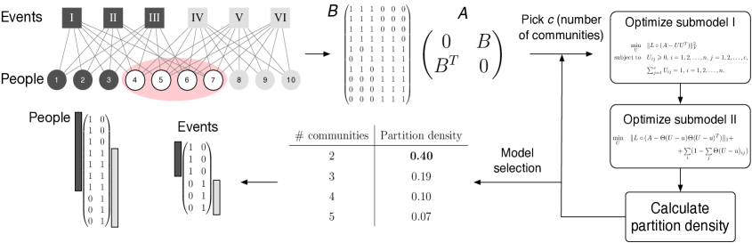
Figure 1: Illustration of wSBMF method. The network consists of events and people and exhibits two overlapping groups where some individuals (4-7) belong to both communities.

2.4 Possible Extensions

The wSBMF model can be naturally extended to $M$-partite networks, whose adjacency matrix can be split into $M\times M$ blocks:

$$A=\left[\begin{array}[]{c c c c c}\vspace{2mm}\mathbf{0}_{\Lambda_{1},\Lambda_{1}}&B_{{\Lambda_{1},\Lambda_{2}}}&\mathbf{0}_{\Lambda_{1},\Lambda_{3}}&\cdots&\mathbf{0}_{\Lambda_{1},\Lambda_{M}}\\ B_{{\Lambda_{1},\Lambda_{2}}}^{T}&\mathbf{0}_{\Lambda_{2},\Lambda_{2}}&B_{{\Lambda_{2},\Lambda_{3}}}&\cdots&\mathbf{0}_{\Lambda_{2},\Lambda_{M}}\vspace{2mm}\\ \mathbf{0}_{\Lambda_{3},\Lambda_{1}}&B_{{\Lambda_{2},\Lambda_{3}}}^{T}&\mathbf{0}_{\Lambda_{3},\Lambda_{3}}&\cdots&\mathbf{0}_{\Lambda_{3},\Lambda_{M}}\vspace{2mm}\\ \vdots&\cdots&\cdots&\cdots&\vdots\vspace{2mm}\\ \vdots&\cdots&\cdots&\cdots&\vdots\vspace{2mm}\\ \mathbf{0}_{\Lambda_{M-1},\Lambda_{1}}&\mathbf{0}_{\Lambda_{M-1},\Lambda_{2}}&\cdots&\mathbf{0}_{\Lambda_{M-1},\Lambda_{M-1}}&B_{{\Lambda_{M-1},\Lambda_{M}}}\vspace{2mm}\\ \mathbf{0}_{\Lambda_{M},\Lambda_{1}}&\mathbf{0}_{\Lambda_{M},\Lambda_{2}}&\cdots&B_{{\Lambda_{M-1},\Lambda_{M}}}^{T}&\mathbf{0}_{\Lambda_{M},\Lambda_{M}}\end{array}\right],$$

where $\mathbf{0}_{\Lambda_{i},\Lambda_{j}}$ is null matrix of size $n_{\Lambda_{i}}\times n_{\Lambda_{j}},$ and

$$B_{\Lambda_{i},\Lambda_{i+1}ab}=\left\{\begin{array}[]{rcl}1,&&\mbox{if}\ a\sim b,\ a\in\Lambda_{i},\,b\in\Lambda_{i+1}\\ 0,&&\mbox{if}\ a\nsim b,\ a\in\Lambda_{i},\,b\in\Lambda_{i+1},\ \ i=1,2,\cdots,M-1.\\ \end{array}\right.$$

In this case, $L$ should be reformulated as:

$$L=\left[\begin{array}[]{c c c c c}\vspace{2mm}\mathbf{0}_{\Lambda_{1},\Lambda_{1}}&\mathbf{I}_{{\Lambda_{1},\Lambda_{2}}}&\mathbf{0}_{\Lambda_{1},\Lambda_{3}}&\cdots&\mathbf{0}_{\Lambda_{1},\Lambda_{M}}\\ \mathbf{I}_{{\Lambda_{2},\Lambda_{1}}}&\mathbf{0}_{\Lambda_{2},\Lambda_{2}}&\mathbf{I}_{{\Lambda_{2},\Lambda_{3}}}&\cdots&\mathbf{0}_{\Lambda_{2},\Lambda_{M}}\vspace{2mm}\\ \mathbf{0}_{\Lambda_{3},\Lambda_{1}}&\mathbf{I}_{{\Lambda_{3},\Lambda_{2}}}&\mathbf{0}_{\Lambda_{3},\Lambda_{3}}&\cdots&\mathbf{0}_{\Lambda_{3},\Lambda_{M}}\vspace{2mm}\\ \vdots&\cdots&\cdots&\cdots&\vdots\vspace{2mm}\\ \vdots&\cdots&\cdots&\cdots&\vdots\vspace{2mm}\\ \mathbf{0}_{\Lambda_{M-1},\Lambda_{1}}&\mathbf{0}_{\Lambda_{M-1},\Lambda_{2}}&\cdots&\mathbf{0}_{\Lambda_{M-1},\Lambda_{M-1}}&\mathbf{I}_{{\Lambda_{M-1},\Lambda_{M}}}\vspace{2mm}\\ \mathbf{0}_{\Lambda_{M},\Lambda_{1}}&\mathbf{0}_{\Lambda_{M},\Lambda_{2}}&\cdots&\mathbf{I}_{{\Lambda_{M},\Lambda_{M-1}}}&\mathbf{0}_{\Lambda_{M},\Lambda_{M}}\end{array}\right],$$

where $\mathbf{I}_{{\Lambda_{i},\Lambda_{j}}}$ is matrix where all entries are one with size $n_{\Lambda_{i}}\times n_{\Lambda_{j}}$.

3 Results

In this section we evaluate the performance of our method using both synthetic and real-world networks.

3.1 Datasets Description

We first discuss the existing bipartite benchmark networks [11]. The benchmark has five communities, each having the same number of nodes. Edges only exist between $\Delta$ and $\Gamma$ with possibility $p_{in}$ if they are in the same community and $p_{out}$ if otherwise. Often, $p_{in}$ is set equal to either $0.5$ or $0.9$ and $p_{out}$ is set as $\alpha p_{in}$, where $\alpha$ varies from $0$ to 1. With increasing $\alpha$, the community structure becomes less clear. Here we propose two new, more realistic benchmark graphs that exhibit overlaps, variable community sizes, and fixed density with different mixing parameters.

• Non-overlapping communities: This class of networks has four communities with the same number of nodes (each with 32 from $\Delta$ and 32 from $\Gamma$). Edges exist only between $\Delta$ and $\Gamma$. On average, each node has $Z_{in}+Z_{out}=16$ edges. In other words, each node in $\Delta$ has $Z_{in}$ neighbors within its own community and $Z_{out}$ ones outside. With decreasing $Z_{out}$, the community structures become clearer.

• Overlapping communities: This class of networks has $c$ communities and the number of nodes in each community can differ from each other. A community $\alpha$ contains $n_{\Delta}^{(\alpha)}$ nodes and $n_{\Gamma}^{(\alpha)}$ ones in $\Delta$ and $\Gamma$ respectively. On average each $\Delta$ node in the community $\alpha$ has $Z_{in}^{(\alpha)}$ $\Gamma$ neighbors in its own community and $Z_{out}^{(\alpha)}$ $\Gamma$ neighbors in other communities. Actually, since we should have $Z_{in}^{(\alpha)}/n_{\Gamma}^{(\alpha)}=Z_{in}^{(\alpha^{\prime})}/n_{\Gamma}^{(\alpha^{\prime})},$ and $Z_{out}^{(\alpha)}/(\sum_{t}n_{\Gamma}^{(t)}-n_{\Gamma}^{(\alpha)})=Z_{in}^{(\alpha^{\prime})}/(\sum_{t}n_{\Gamma}^{(t)}-n_{\Gamma}^{(\alpha^{\prime})}),\ \alpha,\,\alpha^{\prime}=1,2,\ldots c$, it is enough only to give $Z_{in}^{(1)}$ and $Z_{out}^{(1)}$ to generate the network. In our setting there are four communities containing $32$ $\Delta$ nodes and $32$ $\Gamma$ ones in each community. In addition, there are $t$ overlapping $\Delta$ nodes between communities $\alpha$ and $\alpha+1$, $\alpha=1,\,2,\,3$. $Z_{in}^{(1)}$ and $Z_{out}^{(1)}$ are set to $10$ and $6$, respectively.

We also use real-world networks for evaluation.

• Southern women network [29]: This dataset is the network describing the relations between 18 women and 14 social events. Edges only exist between the women and the events, which makes the graph bipartite. There are 89 edges. The network is commonly used as a benchmark for bipartite community detection.

• Senator network: This is the network of 110 US senators connected by voting records for 696 bills. There is an edge between the senator and the bill if the senator voted for the bill. We remove inactive senators who abstained from more than thirty percent of the bills and also the inactive bills which are waived by more than thirty percent of senators. The final dataset contains 96 senators and 690 bills. There are still abstention cases in the network, which are considered as missing values and can be handled by $L$.

3.2 Assessment Standards

Normalized mutual information is used as the standard to evaluate community structure detection performance. The value can be formulated as follows [30]:

$$I_{norm}(M_{1},M_{2})=\frac{\sum\limits_{i=1}^{c}\sum\limits_{j=1}^{c}n_{ij}\ln\frac{n_{ij}n}{n_{i}^{(1)}n_{j}^{(2)}}}{\sqrt{\left(\sum\limits_{i=1}^{c}n_{i}^{(1)}\ln\frac{n_{i}^{(1)}}{n}\right)\left(\sum\limits_{j=1}^{c}n_{j}^{(2)}\ln\frac{n_{j}^{(2)}}{n}\right)}},$$

where $M_{1}$ and $M_{2}$ are the true cluster label and the computed cluster label, respectively; $c$ is the community number; $n$ is the number of nodes; $n_{ij}$ is the number of nodes in the true cluster $i$ that are assigned to the computed cluster $j$; $n_{i}^{(1)}$ is the number of nodes in the true cluster $i$; and $n_{j}^{(2)}$ is the number of nodes in the computed cluster $j$. The larger the values of NMI, the better the graph partitioning results. For overlapping benchmarks we use the generalized normalized mutual information [31].

3.3 Results

We compare our method with the BRIM model [11], which is the only method that we can get the codes, on the synthetic benchmarks. Note the the BRIM method cannot handle overlapping communities and missing values in the network. To show that the problem of detecting overlapping communities in bipartite networks is not trivial and cannot be reduced to the unipartite case, we also compare our method with SBMF model [22] on the two unipartite networks $\Delta$ and $\Gamma$, where the two nodes are connected if they have at least one common neighbor.

In many real scenarios there is background information available. We can incorporate it into the detection process by revising the objective matrix $A$ and the weight matrix $L$ to improve the performance of detection and the interpretability of the results. Specifically, we consider two types of background information for node pairs of the same type (i.e., $\Delta$ or $\Gamma$): (i) existence constraint $C_{e}$: $(i,j)\in C_{e}$ means that nodes $i$ and $j$ are connected; (ii) absence constraint $C_{a}$: $(i,j)\in C_{a}$ means that nodes $i$ and $j$ are not connected.

We only consider incorporating background information on the nodes in $\Delta$ in this paper for simplicity. Given a bipartite network with $n_{\Delta}$ nodes in $\Delta$, there are $n_{\Delta}(n_{\Delta}-1)/2$ pairs of nodes available. We randomly select five percent of pairs for prior information: if the two nodes in one pair have the same community label, we assume that they belong to $C_{e}$, otherwise they belong to $C_{a}$ [32, 33]. The zero matrices $\mathbf{0}_{\Gamma}$ in $A$ and $L$ are revised accordingly:

$$\mathbf{0}_{\Delta\,ij}=\left\{\begin{array}[]{rcl}1,&&\mbox{if}\ (i,\,j)\in C_{e}\\ 0,&&\mbox{otherwise},\end{array}\right.$$ (6)

where $\mathbf{0}_{\Delta}$ is the submatrix in $A$.

$$\mathbf{0}_{\Delta\,ij}=\left\{\begin{array}[]{rcl}\gamma,&&\mbox{if}\ (i,\,j)\in C_{e}\ \mbox{or}\ (i,\,j)\in C_{a}\\ 0,&&\mbox{otherwise},\end{array}\right.$$ (7)

where $\mathbf{0}_{\Delta}$ is the submatrix in $L$. We set $\gamma$ equal to $1$.

The results are shown in Figs. 2 and 3. They show that the wSBMF method is much better than SBMF on unipartite networks, indicating the nonreducible property of community detection problem in bipartite networks, and it also performs better than BRIM in non-overlapping community benchmark graphs. Our method can identify reasonable number of communities, and the background information can significantly improve the results.

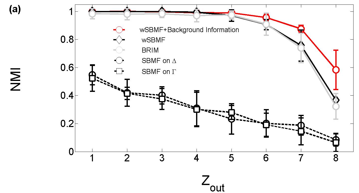
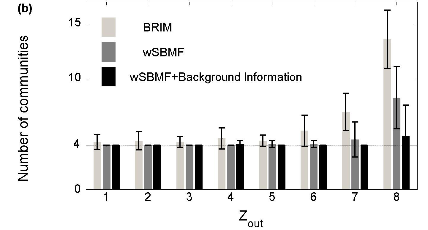
Figure 2: Performance of BRIM and wSBMF on the bipartite networks, SBMF on the monopartite networks, and the number of communities estimated by BRIM and wSBMF on non-overlapping networks. We randomly select five percent of pairs in $\Delta$ for background information.

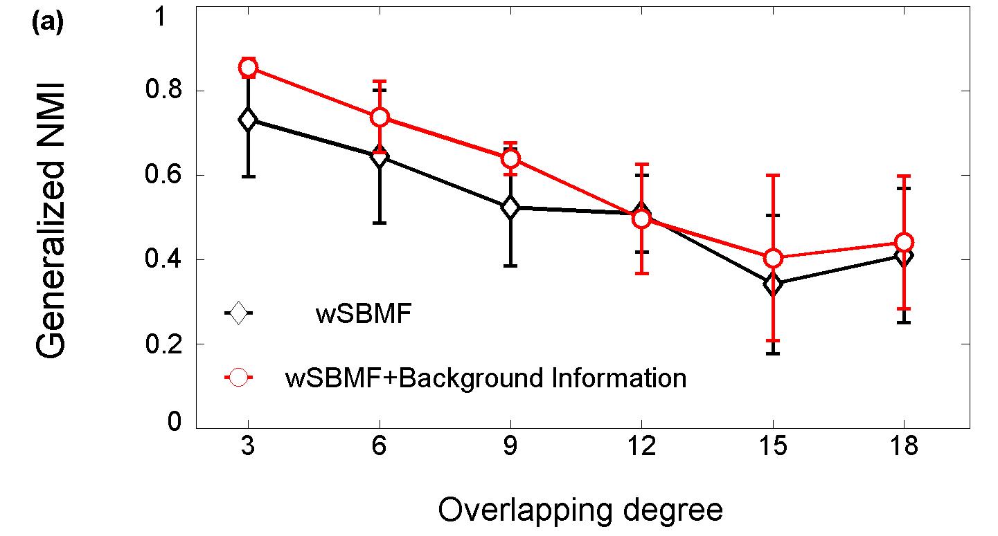
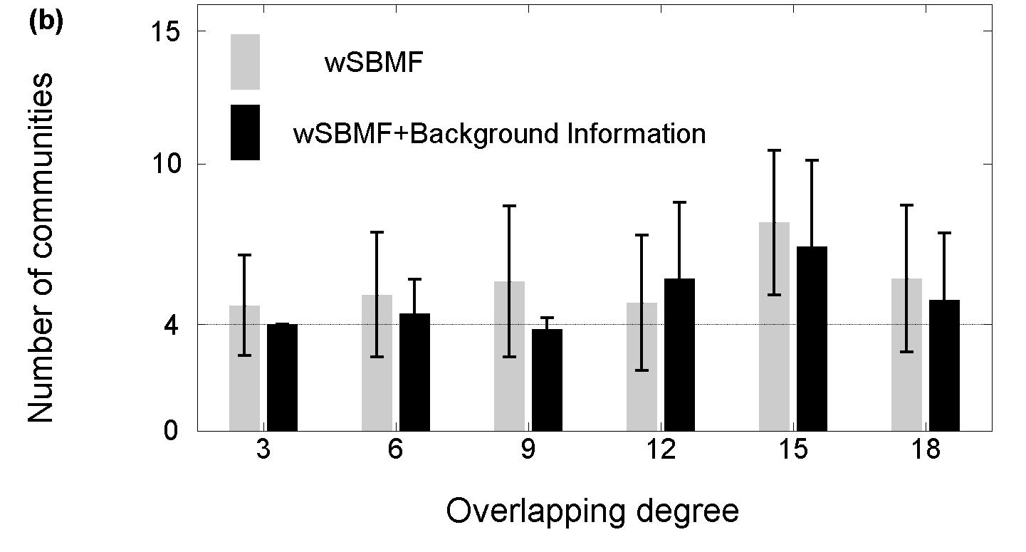
Figure 3: Performance of wSBMF and the number of communities estimated by SBMF on overlapping networks. We randomly select five percent of pairs in $\Delta$ for background information.

We also evaluate the method on the southern women network and the senator network. Fig. 4 shows the results of partition density under different community numbers on the two networks, and the most appropriate number is 2 for both of them. For the southern women network, the result is very similar to that in [29], where there are two groups in women, women $1-9$ and $9-18$. For the senator network, the result is consistent with American two-party politics. Fig. 5 shows the result of community structure on the women network detected by wSBMF. We also use exponential entropy $e^{H_{i}},i=1,2,\ldots,n_{\Delta}$ [34], to analyze the strength of women’s community memberships, where

$$H_{i}=-\sum_{j=1}^{2}U_{ij}\log U_{ij},i=1,2,\ldots,n_{\Delta}.$$

The result is given in Fig. 6.

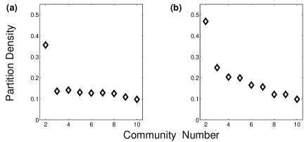
Figure 4: Averaged partition density of wSBMF versus community number on (a) women network and (b) senator network.

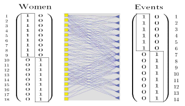
Figure 5: Communities detected by wSBMF model in the women network. There are no outliers and overlapping nodes.

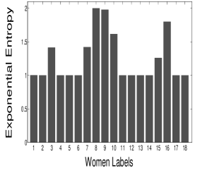
Figure 6: Exponential entropy of women. Higher value means fuzzier membership degree.

4 Discussion

In this paper we have shown how to apply symmetric binary matrix factorization and partition density to find communities in bipartite networks. The model is parameter free, easy to implement, and flexible enough to incorporate background information. Experimental results on both the synthetic and real-world networks demonstrate the effectiveness of the proposed method.

There are two interesting problems for future work: (i) extension of the method to weighted bipartite networks and directed bipartite networks; and (ii) theoretical investigation on partition density and algorithm design for its direct optimization.

Appendix

Summarization of Algorithm 1 and 2. We set the iteration number $\mbox{C}_{1}$ equal to 10 and the iteration number $\mbox{C}_{2}$ equal to 100.

Algorithm 1 Nonnegative Matrix Factorization (Alternative Least Squares Error)

0:  $B,\mbox{C}_{1}$

0:  $U_{1},U_{2}$

1:  Initialize elements of $U_{1}$ with nonnegative random numbers drawn from $[0,1]$.

2:  for $t=1:\mbox{C}_{1}$ do

3:     Solve for $U_{2}$ in equation $U_{1}^{T}U_{1}U_{2}=U_{1}^{T}A$

4:     $U_{2}=\max(U_{2},0)$

5:     Solve for $U_{2}$ in equation $U_{2}U_{2}^{T}U_{1}^{T}=U_{2}A^{T}$

6:     $U_{1}=\max(U_{1},0)$

7:  end for

Algorithm 2 Weighted Symmetric Nonnegative Matrix Factorization (Multiplicative Updates)

0:  $A,U,\mbox{C}_{2}$

0:  $U$

1:  for $t=1:\mbox{C}_{2}$ do

2:     $\displaystyle U:=U\circ\frac{\left[(L\circ A)U\right]}{\left[L\circ(UU^{T})U\right]}$

3:  end for

4:  $\displaystyle{U_{ij}:=\frac{U_{ij}}{\sum_{j}U_{ij}}},i\,=1,2,\cdots,n$

References

• [1] Girvan M and Newman M E J, 2002 Proceedings of the National Academy of Sciences 99(12) 7821–7826
• [2] Newman M E J and Girvan M, 2004 Physical review E 69(2) 026113
• [3] Dreze M, Carvunis A R, Charloteaux B, Galli M, Pevzner S J, Tasan M, Ahn Y Y, Balumuri P, Barabási A L, Bautista V, et al., 2011 Science 333(6042) 601–607
• [4] Newman M E J, 2006 Proceedings of the National Academy of Sciences 103(23) 8577–8582
• [5] Ahn Y Y, Bagrow J P, and Lehmann S, 2010 Nature 466(7307) 761–764
• [6] Gulbahce N and Lehmann S, 2008 BioEssays 30(10) 934–938
• [7] Porter M A, Onnela J P, and Mucha P J, 2009 Notices of the AMS 56(9) 1082–1097
• [8] Fortunato S, 2010 Physics Reports 486(3) 75–174
• [9] Wu X and Liu Z, 2008 Physica A 387 623–630
• [10] Weng L, Menczer F, and Ahn Y Y, 2013 arXiv preprint arXiv:1306.0158
• [11] Barber M J, 2007 Physical Review E 76(6) 066102
• [12] Du N, Wang B, Wu B, and Wang Y, 2008 In Web Intelligence and Intelligent Agent Technology, 2008. WI-IAT’08. IEEE/WIC/ACM International Conference on, volume 1, 176–179. IEEE
• [13] Zhan W, Zhang Z, Guan J, and Zhou S, 2011 Physical Review E 83(6) 066120
• [14] Lehmann S, Schwartz M, and Hansen L K, 2008 Physical Review E 78(1) 016108
• [15] Liu X and Murata T, 2009 In Web Intelligence and Intelligent Agent Technologies, 2009. WI-IAT’09. IEEE/WIC/ACM International Joint Conferences on, volume 1, 50–57. IET
• [16] Lind P G, González M C, and Herrmann H J, 2005 Physical review E 72(5) 056127
• [17] Lind P G and Herrmann H J, 2007 New Journal of Physics 9(7) 228
• [18] Ahn Y Y, Ahnert S E, Bagrow J P, and Barabási A L, 2011 Scientific reports 1
• [19] Jeong H, Tombor B, Albert R, Oltvai Z N, and Barabási A L, 2000 Nature 407(6804) 651–654
• [20] Newman M E J, 2001 Physical review E 64(1) 016132
• [21] Zhou T, Ren J, Medo M, and Zhang Y C, 2007 Physical Review E 76(4) 046115
• [22] Zhang Z Y, Wang Y, and Ahn Y Y, 2013 Physical Review E 87(6) 062803
• [23] Lee H, Yoo J, and Choi S, 2010 Signal Processing Letters, IEEE 17(1) 4–7
• [24] Paatero P and Tapper U, 1994 Environmetrics 5(2) 111–126
• [25] Berry M W, Browne M, Langville A N, Pauca V P, and Plemmons R J, 2007 Computational Statistics & Data Analysis 52(1) 155–173
• [26] Zhang Z Y, Ding C, Li T, and Zhang X, 2007 In Data Mining, 2007. ICDM 2007. Seventh IEEE International Conference on, 391–400. IEEE
• [27] Zhang Z Y, Li T, Ding C, Ren X, and Zhang X, 2010 Data Mining and Knowledge Discovery 20(1) 28–52
• [28] Zhang Z Y, 2012 In Data Mining: Foundations and Intelligent Paradigms, 99–134. Springer
• [29] Davis A, Gardner B B, and Gardner M R, 1941 Deep south. University of Chicago Press Chicago
• [30] Strehl A and Ghosh J, 2002 Journal of Machine Learning Research 3 583–617
• [31] Lancichinetti A, Fortunato S, and Kertész J, 2009 New Journal of Physics 11(3) 033015
• [32] Zhang Z Y, 2013 EPL (Europhysics Letters) 48005+
• [33] Gopalan P K and Blei D M, 2013 Proceedings of the National Academy of Sciences 110(36) 14534–14539
• [34] Campbell L, 1966 Probability Theory and Related Fields 5(3) 217–225