Effective theory for the non-rigid rotor in an electromagnetic field: Toward accurate and precise calculations of E2 transitions in deformed nuclei

Abstract

We present a model-independent approach to electric quadrupole transitions of deformed nuclei. Based on an effective theory for axially symmetric systems, the leading interactions with electromagnetic fields enter as minimal couplings to gauge potentials, while subleading corrections employ gauge-invariant non-minimal couplings. This approach yields transition operators that are consistent with the Hamiltonian, and the power counting of the effective theory provides us with theoretical uncertainty estimates. We successfully test the effective theory in homonuclear molecules that exhibit a large separation of scales. For ground-state band transitions of rotational nuclei, the effective theory describes data well within theoretical uncertainties at leading order. In order to probe the theory at subleading order, data with higher precision would be valuable. For transitional nuclei, next-to-leading order calculations and the high-precision data are consistent within the theoretical uncertainty estimates. We also study the faint inter-band transitions within the effective theory and focus on the $E2$ transitions from the $0^{+}_{2}$ band (the “$\beta$ band”) to the ground-state band. Here, the predictions from the effective theory are consistent with data for several nuclei, thereby proposing a solution to a long-standing challenge.

I Introduction

Our understanding of deformed nuclei in the rare-earth and actinide regions of the nuclear chart is largely based on the geometric collective models Bohr (1952); Bohr and Mottelson (1953); Eisenberg and Greiner (1970a); Bohr and Mottelson (1975); Hess et al. (1980); Próchniak and Rohoziński (2009); Rowe and Wood (2010), and the algebraic collective models Arima and Iachello (1975); Matsuo (1984). For even-even nuclei, these models employ quadrupole degrees of freedom (and an additional $s$ boson in the interacting boson model Iachello and Arima (1987)). The collective models depend on a small numbers of parameters. They describe the key features of deformed nuclei, namely low-energy spectra consisting of rotational bands on top of vibrational band heads, with strong $E2$ intra-band transitions, and much weaker inter-band transitions. However, some finer details are not well described by the collective models, and the accurate description of inter-band electromagnetic transition strengths is a particular challenge. As an example we mention the overprediction (by factors of 2 to 10) of $E2$ transitions between the rotational band on top of the $0^{+}_{2}$ vibrational band head (historically called the “$\beta$ band”) and the ground-state band for well-deformed nuclei Garrett (2001); Aprahamian (2004); Rowe and Wood (2010). This situation is similar for transitional nuclei at the border between sphericity and deformation. Here, the models based on the $X(5)$ solution by Iachello (2001) of the Bohr Hamiltonian tend to overpredict electromagnetic inter-band transitions Zamfir et al. (1999); Casten and Zamfir (2001); Krücken et al. (2002); Tonev et al. (2004).

In recent years, computationally tractable approaches to collective models Rowe (2004); Rowe et al. (2009) led to a better understanding of geometric models and their parameter space Caprio (2005). However, it seems that changes to the Bohr Hamiltonian, e.g. by studying non-separable potentials Caprio (2009) or by considering other solutions Inci et al. (2011), do not overcome the deficiencies for the inter-band transitions. We also note that a variety of approaches addressed other shortcomings of the collective models by focusing on tri-axial deformations Allmond et al. (2008), or inclusion of isovector modes Bentz et al. (2011, 2014), see Ref. Matsuyanagi et al. (2010) for a review of present challenges.

Increasing the complexity of collective models, e.g. through the addition of more terms, can lead to an undesirable proliferation of parameters and a loss of predictive power. This unattractive feature of modeling can partly be overcome by effective field theories (EFTs). An EFT is based on symmetry principles alone and exploits a separation of scales for the systematic construction of Hamiltonians based on a power counting. In this way, an increase in the number of parameters (i.e. low-energy constants that need to be adjusted to data) goes hand in hand with an increase in precision, and thereby counters the loss of predictive power. Furthermore, this systematic increase in precision makes it possible to estimate theoretical uncertainties, see Furnstahl et al. (2015) for a recent review. Finally, the EFT approach also helps us to identify inherent limitations that are due to the breakdown scale of the theory.

The successful reproduction of the low-energy spectra of deformed nuclei strongly suggests that the geometric collective model correctly captures key aspects such as relevant degrees of freedom and the interaction between them. This picture is also obtained in a model-independent approach to deformed nuclei based on EFT Papenbrock (2011); Zhang and Papenbrock (2013); Papenbrock and Weidenmüller (2014).

The overprediction of the inter-band transition strengths in collective models thus leads us to scrutinize the operators that are employed in the calculations of $E2$ transition strengths. The Bohr Hamiltonian models the nucleus as an incompressible liquid drop with quadrupole surface oscillations. These corresponding five degrees of freedom can be mapped onto three Euler angles (describing overall rotations of the nucleus) and two deformation parameters (describing vibrations in the body-fixed coordinate system). In this model, $E2$ transitions are computed from the quadrupole operator. This approach to electric transitions in deformed nuclei seems to be motivated by Siegert’s theorem Siegert (1937), which allows one to employ the density instead of the current operator in the computation of some transition rates, see e.g. Ref. Greiner et al. (1997). We recall that the derivation of Siegert’s theorem is based on gauge invariance and starts from gauging momentum operators Sachs and Austern (1951). Thus the applicability of Siegert’s theorem is not obvious for the collective models that employ quadrupole operators for momenta (as opposed to vectors).

The identification of the transition operator is even more challenging for the algebraic models because of the lack of a geometric picture. For the calculation of electromagnetic transition strengths, these models employ operators that couple the basic degrees of freedom to a spherical tensor whose rank equals the desired multipole order. For a recent analysis of this approach, we refer the reader to Ref. Ionescu and Hategan (2012).

In this work we study the electromagnetic coupling of deformed nuclei within an effective theory motivated by similar approaches to other nuclear systems, see Refs. Pastore et al. (2009); Kölling et al. (2009); Hammer and Phillips (2011); Grießhammer et al. (2012); Hagen et al. (2013); Girlanda et al. (2014) for recent examples. In contrast to more phenomenological models, the consistent treatment of Hamiltonians and currents is a highlight of effective theories. As we will see, coupling the non-rigid rotor to electromagnetic fields in a model-independent way is an interesting problem in itself. Perhaps somewhat surprisingly, we are not aware of any literature addressing this problem. Our approach reproduces the strong intra-band transitions that are also described accurately by the collective models. For the weaker inter-band transitions, the effective theory approach yields a much improved description of data and thereby suggests steps toward overcoming some limitations of the geometric and algebraic collective models. Finally, the effective theory approach also permits us to give theoretical uncertainty estimates and thereby facilitates a meaningful comparison with data. As we will see, this comparison also suggests that data with higher precision for $E2$ transitions would be very valuable.

Ultimately, a microscopic theory of deformed nuclei must be based on fermionic constituents. Nuclear mean field and density functional theories (see Refs Nazarewicz (1994); Frauendorf (2001) for reviews), are making impressive predictions of rotational bands and moments of inertia Sheikh et al. (2008); Nikšić et al. (2011), with new projection techniques being proposed Duguet (2015). In light $p$-shell nuclei, ab initio approaches are now addressing the emergent behavior of rotational collective motion Caprio et al. (2013); Dytrych et al. (2013). Recently, fermionic approaches have also been used to constrain parameters of collective models Nomura et al. (2008).

This paper is organized as follows. In Sect. II we briefly review the effective theory for axially deformed nuclei. The electromagnetic coupling of the effective theory is described in Sect. III. Section IV presents the results for intra-band $E2$ transitions and compares them to data on rotational and transitional nuclei. A somewhat surprising result is that much of the available data lacks the precision to challenge the effective theory. Sections V and VI include quadrupole degrees of freedom for the description of inter-band transitions. Comparison to data shows that the effective theory accounts well for these faint transitions. Finally, we present our summary.

II Effective theory for the axially symmetric non-rigid rotor

In this Section we briefly review the effective theory for deformed nuclei Papenbrock (2011); Zhang and Papenbrock (2013); Papenbrock and Weidenmüller (2014). The presentation in this paper aims at being more intuitive and less technical, though. We first focus on the lowest-energy phenomena and thus on the axially symmetric non-rigid rotor. The coupling to vibrations is considered in Sect. V.

II.1 Low-energy degrees of freedom

The effective theory is based on the emergent symmetry breaking from the rotational symmetry of the group ${\cal G}=\rm{SO(3)}$ to axial symmetry of the subgroup ${\cal H}=\rm{SO(2)}$. Thus, the Nambu-Goldstone modes parameterize the coset Coleman et al. (1969); Callan et al. (1969); Leutwyler (1994); Román and Soto (1999); Hofmann (1999); Kämpfer et al. (2005); Brauner (2010) ${\cal G}/{\cal H}=\rm{SO(3)/SO(2)}$ which is isomorph to the two-sphere. This agrees with our intuition: the orientation of an axially symmetric object is defined by two Euler angles or, equivalently, by the direction of its symmetry axis. In a finite system, the symmetry breaking has an emergent character, and (quantized) zero modes take the place of Nambu-Goldstone modes Leutwyler (1987); Hasenfratz and Niedermayer (1993); Papenbrock and Weidenmüller (2014). In our case, the polar and azimuthal angles $\theta$ and $\phi$ (also labeled compactly as $\Omega$) parameterize the two-sphere, i.e., the radial unit vector

$$\mathbf{e}_{r}\equiv\left(\begin{array}[]{c}\sin{\theta}\cos{\phi}\\ \sin{\theta}\sin{\phi}\\ \cos{\theta}\end{array}\right)$$ (1)

indicates the direction of the symmetry axis of the non-rigid rotor. Thus, the effective theory for this system is equivalent to that of a particle on the two-sphere.

The velocity of the orientation vector $\mathbf{e}_{r}$ is the time derivative

$$\begin{split}d_{t}\mathbf{e}_{r}&=\dot{\theta}\mathbf{e}_{\theta}+\dot{\phi}\sin{\theta}\mathbf{e}_{\phi}\\ &\equiv v_{\theta}\mathbf{e}_{\theta}+v_{\phi}\mathbf{e}_{\phi}\equiv\mathbf{v}.\end{split}$$ (2)

This vector lies in the plane tangent to the two-sphere at $\Omega$. Here and in what follows, we employ dots to denote time derivatives. The low-energy Lagrangian is a scalar function of the velocity vector alone and does not depend on the vector $\mathbf{e}_{r}$ because of the emergent symmetry breaking. To make progress, we need to understand the behavior of $\mathbf{v}$ under rotations, and establish a power counting. With these two ingredients in hand, we then construct the most general Lagrangian that is consistent with rotational symmetry and at a given order of the power counting.

II.2 Rotational invariance

Under a rotation $r\equiv r(\alpha,\beta,\gamma)=\exp{(-i\alpha\hat{J}_{z})}\exp{(-i\beta\hat{J}_{y})}\exp{(-i\gamma\hat{J}_{z})}$, parameterized by the three Euler angles $(\alpha,\beta,\gamma)$, the angles $\theta$ and $\phi$ transform non-linearly into $\theta^{\prime}$ and $\phi^{\prime}$. This constitutes a nonlinear realization of SO(3). It is interesting to comapre this with Bohr’s approach to deformed nuclei Bohr (1952). Bohr starts from a linear representation of SO(3) by choosing deformation parameters as coefficients of spherical harmonics. The transformation to the body-fixed coordinate system then introduces a nonlinear realization of SO(3) in terms of three rotation angles and two deformation parameters. The rotation $r$ transforms the velocity vector $\mathbf{v}(\Omega)$ (or any vector in the tangent plane) into the vector $\mathbf{v}^{\prime}(\Omega^{\prime})$ that lies in the tangent plane at $\Omega^{\prime}$. It is clear that the mapping from $\mathbf{v}$ to $\mathbf{v}^{\prime}$ is equivalent to a SO(2) rotation in the tangent plane by an angle $\chi=\chi(\alpha,\beta,\gamma;\Omega)$ that is a complicated function of the Euler angles and the original coordinates $\Omega$. Details are given in Ref. Papenbrock (2011).

At this point it is useful to introduce spherical components of the velocity inside the tangent plane as

$$v_{\pm}\equiv{1\over\sqrt{2}}(v_{\theta}\pm iv_{\phi})\ .$$ (3)

Under a rotation by the Euler angles $(\alpha,\beta,\gamma)$ the vector $\mathbf{v}$ transforms as

$$v_{\pm}\rightarrow e^{\mp i\chi}v_{\pm}.$$ (4)

Thus, under an SO(3) transformation, vectors in the tangent plane formally transform under an SO(2) transformation, and any Lagrangian build from elements in the tangent plane that is formally invariant under SO(2), is in fact invariant under SO(3).

For the general construction of invariant Lagrangians, we must also consider time derivatives of vectors in the tangent plane. The resulting vectors may not lie in the tangent plane. Thus, the ordinary time derivative needs to be replaced by the covariant derivative

$$D_{t}\equiv d_{t}-i\dot{\phi}\cos{\theta}\hat{J}_{z},$$ (5)

which is the projection onto the tangent plane of the ordinary time derivative.

Let $L$ denote a rotationally invariant Lagrangian in the velocities $v_{\pm}$. The application of Noether’s theorem yields the angular momentum $\mathbf{I}$ as the conserved quantity Papenbrock (2011). Its spherical components $I_{+}$, $I_{0}$ and $I_{-}$ are

$$\begin{split}I_{+1}&=-{1\over\sqrt{2}}e^{i\phi}(ip_{\theta}-p_{\phi}\cot{\theta})\\ I_{0}&=p_{\phi}\\ I_{-1}&=-{1\over\sqrt{2}}e^{-i\phi}(ip_{\theta}+p_{\phi}\cot{\theta}).\end{split}$$ (6)

Here

$$p_{\theta}\equiv\partial_{\dot{\theta}}L\qquad p_{\phi}\equiv\partial_{\dot{\phi}}L$$ (7)

denotes the canonical momenta. The squared angular momentum is

$$\mathbf{I}^{2}=p_{\theta}^{2}+\frac{p_{\phi}^{2}}{\sin^{2}{\theta}}.$$ (8)

This construction of the Lagrangian is particularly useful when further degrees of freedom are coupled to the axially symmetric rotor.

II.3 Power counting and the rotational Hamiltonian

The leading-order (LO) rotationally invariant Lagrangian

$$L_{\rm LO}=C_{0}v_{+1}v_{-1}=\frac{C_{0}}{2}(\dot{\theta}^{2}+\dot{\phi}^{2}\sin^{2}{\theta})$$ (9)

is quadratic in the velocities $v_{\pm}$. It is equivalent to that of a particle restricted to move on the two-sphere, or to that of a rigid rotor. Here, $C_{0}$ is a low-energy constant and corresponds to the effective moment of inertia. This parameter of our theory must be fixed by data.

For the power counting, we need to introduce relevant energy scales. Let $\xi$ denote the low-energy scale associated with rotations. Then, $\xi\sim 80$ keV and $\xi\sim 40$ keV for deformed rare-earth nuclei and actinides respectively. The breakdown scale $\omega$ of the effective theory coincides with the onset of vibrational excitations and is of the order of 1 MeV and 0.6 MeV for rare-earth nuclei and actinides respectively. Thus, $\xi/\omega\approx 1/10$ is a conservative estimate.

The LO Lagrangian and the time derivatives (such as the velocities $v_{\pm}$) are of order $\xi$. Thus,

$$v_{\pm}\sim\dot{\phi}\sim\dot{\theta}\sim\xi\qquad C_{0}\sim\xi^{-1}.$$ (10)

A Legendre transformation of the LO Lagrangian yields the LO Hamiltonian

$$H_{\rm LO}=\frac{1}{2C_{0}}\left(p_{\theta}^{2}+\frac{p_{\phi}^{2}}{\sin^{2}{\theta}}\right)=\frac{1}{2C_{0}}\mathbf{I}^{2}.$$ (11)

The quantization is standard, and the angular momentum $\mathbf{I}$ becomes the angular momentum operator $\hat{\mathbf{I}}$ with spherical components Varshalovich et al. (1988)

$$\begin{split}\hat{I}_{+1}&=-{1\over\sqrt{2}}e^{i\phi}\left(\partial_{\theta}+i\cot{\theta}\partial_{\phi}\right)\\ \hat{I}_{0}&=-i\partial_{\phi}\\ \hat{I}_{-1}&=-{1\over\sqrt{2}}e^{-i\phi}\left(\partial_{\theta}-i\cot{\theta}\partial_{\phi}\right).\end{split}$$ (12)

The squared angular momentum is

$$\hat{\mathbf{I}}^{2}=\hat{I}_{0}^{2}-\hat{I}_{+}\hat{I}_{-}-\hat{I}_{-}\hat{I}_{+}.$$ (13)

We also recall that

$$\hat{\mathbf{I}}=\mathbf{e}_{r}\times\left(-i\mathbf{\nabla}_{\Omega}\right)\ ,$$ (14)

with

$$\mathbf{\nabla}_{\Omega}=\mathbf{e}_{\theta}\partial_{\theta}+\mathbf{e}_{\phi}{1\over\sin\theta}\partial_{\phi}$$ (15)

being the angular derivative in the tangent plane Varshalovich et al. (1988). We note that $-i\mathbf{\nabla}_{\Omega}$ is not an Hermitian operator.

The eigenfunctions of the Hamiltonian (11) are spherical harmonics $Y_{IM}(\Omega)$ with eigenvalues

$$\hat{H}_{\rm LO}Y_{IM}(\theta,\phi)={I(I+1)\over 2C_{0}}Y_{IM}(\theta,\phi)$$ (16)

Higher-order corrections to the LO Lagrangian (9) include terms with higher powers of $\mathbf{I}^{2}$. At next-to-leading order (NLO) the Lagrangian becomes $L_{\rm LO}+L_{\rm NLO}$ with

$$L_{\rm NLO}={C_{2}\over 4}\left(\mathbf{I}^{2}\right)^{2}.$$ (17)

Thus, the corresponding Hamiltonian is $H_{\rm LO}+H_{\rm NLO}$ with

$$H_{\rm NLO}=-{C_{2}\over C_{0}^{2}}\left(H_{\rm LO}\right)^{2}=-{C_{2}\over 4C_{0}^{3}}\left(\mathbf{I}^{2}\right)^{2}\ ,$$ (18)

and the spectrum becomes

$$E(I)={I(I+1)\over 2C_{0}}-{C_{2}\over 4C_{0}^{4}}\left(I(I+1)\right)^{2}\ .$$ (19)

This deviation from the rigid-rotor behavior is due to omitted physics at the energy scale $\omega$ of vibrations. From the expression for the NLO Hamiltonian (18) it is clear that $C_{2}$ has units of energy^-3. The scaling is Papenbrock (2011)

$$C_{2}\sim C_{0}/\omega^{2},$$ (20)

and consequently, the ratio of the NLO correction to the LO contribution of the energy scales as

$$\frac{\langle\hat{H}_{\rm NLO}\rangle}{\langle\hat{H}_{\rm LO}\rangle}\sim\left(\frac{\xi}{\omega}\right)^{2}I(I+1).$$ (21)

Thus, the effective theory of the axially symmetric non-rigid rotor is identical to the variable-moment-of-inertia model Mariscotti et al. (1969); Scharff-Goldhaber et al. (1976), and the spectrum consists of increasing powers of $I(I+1)$. It is important to notice that according to Eq. (21), the effective theory is expected to break down at spins of magnitude $\omega/\xi$, i.e. when the second term in Eq. (19) becomes as large as the first term. For a given nucleus, an estimate for the breakdown spin can be obtained by employing the LECs $C_{0}$ and $C_{2}$. The result is the estimate $\sqrt{C_{0}^{3}/C_{2}}$. For the rotors listed in Table 1, this estimate usually excceds the general estimate $\omega/\xi$.

Table 1 below shows values $C_{0}\xi$, $(C_{2}/C_{0})\omega^{2}$, $(\xi/\omega)^{2}$, and $C_{2}/C_{0}^{3}$ from the description of the ground-state bands of the homonuclear molecules $N_{2}$ and $H_{2}$, the rotational nuclei ²³⁶U, ¹⁷⁴Yb, ^166,168Er, and ¹⁶²Dy, and the transitional nuclei ¹⁸⁸Os, ¹⁵⁴Gd, ¹⁵²Sm, and ¹⁵⁰Nd, respectively. Here, $\xi$ is the excitation energy of the lowest $2^{+}$ state and $\omega$ is the excitation energy of the lowest vibrational state. The values of $C_{0}$ and $C_{2}$ are obtained from a simultaneous fit to the lowest $2^{+}$ and $4^{+}$ levels to Eq. (19), respectively. For a rigid rotor, $C_{0}\xi=3$, $\xi/\omega=0$, and $C_{2}/C_{0}^{3}=0$. Table 1 shows that the ratios $(C_{2}/C_{0})\omega^{2}$ are of natural size, i.e. of order one, for the considered molecules and nuclei, and that the ratios $C_{2}/C_{0}^{3}$ are consistent with (but systematically smaller than) the scaling estimate $(\xi/\omega)^{2}$. This suggests that the breakdown scale is higher than the conservative estimate of $\omega$. Still, the values for the LEC $C_{2}$ are consistent with scaling estimates. Clearly the molecule N₂ is very close to the rigid-rotor limit. The comparison suggests that the molecule H₂ is as non-rigid a rotor as the nuclei ²³⁶U, ¹⁷⁴Yb and ¹⁶⁸Er. The transitional nuclei ¹⁸⁸Os, ¹⁵⁴Gd, ¹⁵²Sm, and ¹⁵⁰Nd exhibit even larger deviations from the rigid-rotor limit.

System	$C_{0}\xi$	${C_{2}\over C_{0}}\omega^{2}$	$(\xi/\omega)^{2}$	$C_{2}/C_{0}^{3}$	$b/a$
N2	$3.00$	$2.1$	$0.000026$	$0.000006$	$-0.000011$
H2	$2.99$	$2.2$	$0.0062$	$0.0015$	$0.0022$
236U	$2.99$	$2.3$	$0.0043$	$0.0011$	$-$
174Yb	$2.99$	$3.4$	$0.0026$	$0.0010$	$-$
168Er	$2.99$	$1.0$	$0.0094$	$0.0010$	$-$
166Er	$2.98$	$1.6$	$0.011$	$0.0020$	$-$
162Dy	$2.98$	$1.9$	$0.0083$	$0.0017$	$-$
154Sm	$2.97$	$5.2$	$0.0056$	$0.0033$	$-$
188Os	$2.91$	$1.5$	$0.06$	$0.012$	$0.008$
154Gd	$2.88$	$3.3$	$0.033$	$0.013$	$0.006$
152Sm	$2.88$	$3.5$	$0.032$	$0.013$	$0.003$
150Nd	$2.85$	$3.6$	$0.037$	$0.017$	$0.011$

Table 1: Dimensionless ratios of LECs and energy scales. The LECs $C_{0}$ and $C_{2}$ are obtained from the $2^{+}$ and $4^{+}$ levels of ground-state band for molecules and nuclei considered in this work. The ratio $\xi/\omega$ measures the energy scales of rotations and vibrations. For a rigid rotor $C_{0}\xi=3$, $\xi/\omega=0$, and $C_{2}/C_{0}^{3}=0$. The ratio $b/a$ measures subleading corrections to transition quadrupole moments and is similar in size as the subleading energy correction $C_{2}/C_{0}^{3}$. A dash indicates that the experimental data is not precise enough to determine subleading corrections.

Within an effective field theory for emergent symmetry breaking in finite systems Papenbrock and Weidenmüller (2014), vibrations enter as the quantized Nambu-Goldstone modes. The inclusion of vibrations into the theory pushes the breakdown scale $\Lambda$ to higher energies. We have to distinguish two cases. In the first case, $\Lambda$ is set by the appearance of new degrees of freedom. In nuclei, these are pairing effects, and $\Lambda\approx 2$ to 3 MeV. In molecules these are electronic excitations. The second case concerns the breakdown of the effective theory due to a restoration of spherical symmetry at large excitation energies. Indeed, for energies $\Lambda\sim\omega^{2}/\xi$, the amplitude of vibrations approaches the scale of the static deformation $\sim\xi^{-1/2}$. In nuclei $\omega^{2}/\xi\approx 5$ to 10 MeV, and the breakdown scale is thus given by the onset of new degrees of freedom.

III Coupling to electromagnetic fields

In this Section, we couple the axially-symmetric non-rigid rotor to electromagnetic fields. In leading order, minimal couplings of the gauge fields describe the electromagnetic interaction, and non-minimal couplings enter as subleading corrections. For the long-wavelength $E2$ transitions we are interested in, our approach is more technical than, and differs from, the usual approach taken for the collective models. The usual approach is motivated by the result of Siegert’s theorem, that allows one to employ density operators instead of current operators in transition matrix elements, see Eisenberg and Greiner (1970b) for example. While it is not obvious how to derive this result for the quadrupole degrees of freedom of the collective models, Siegert’s theorem is expected to hold in leading order, i.e. for the strong intra-band transitions. We recall that Mikhailov (1964, 1966) employed the quadrupole operator in the computation of the electromagnetic transition strengths, and the resulting formulas are well known and widely used Bohr and Mottelson (1975). However, this approach fails to describe the order of magnitude for the faint inter-band transitions.

Thus, it is interesting to more formally develop the electromagnetic theory of the rotor. Within an effective theory one consistently relates currents to the underlying Hamiltonian. We also note that Siegert’s theorem does not apply to magnetic transitions Austern and Sachs (1951). The importance of $M1$ transitions is another motivation for carrying out the formal development.

Deriving the electromagnetic couplings for non-relativistic many-body systems from first principles is no easy task Fröhlich and Studer (1993), see also Kämpfer et al. (2005) for a related study within effective field theory. Here, we follow a simpler path (at the possible cost of additional LECs). Within an EFT one writes down all gauge-invariant couplings that are consistent with the underlying symmetries (rotations, time reversal, and parity), and develops a power counting, see Pastore et al. (2009); Kölling et al. (2009); Hammer and Phillips (2011); Grießhammer et al. (2012); Hagen et al. (2013); Girlanda et al. (2014) for recent examples. This introduces minimal couplings (or minimal substitution) and non-minimal couplings.

Before we follow this formal path, however, we briefly consider a simple three-dimensional system that reduces to the effective theory under consideration if a “radial” degree of freedom is frozen (or integrated out). This will give us insights into how to gauge the collective degrees of freedom we are dealing with. Throughout this Section we work in the Coulomb gauge and set the scalar electric potential to zero.

III.1 Instructive example

Let us consider a particle of charge $q$ and mass $m$ in a spherically-symmetric potential $V(r)$ that effectively confines the particle to a region of thickness $\rho\ll R$ around $r\approx R$. The Hamiltonian is

$$\hat{H}=-{\hbar^{2}\over 2m}\Delta+V(r),$$ (22)

with eigenfunctions $\psi(r,\theta,\phi)=\langle r\theta\phi|NIM\rangle=[u_{N}(r)/r]Y_{IM}(\theta,\phi)$. The rotational excitations are of order $\hbar^{2}l(l+1)/(2mR^{2})$, and much smaller than radial excitations, which are of order $\hbar^{2}/(2m\rho^{2})$. Thus, the low-energy spectrum are rotational bands on top of band heads from radial excitations, and the effective theory developed in the previous Section applies. In what follows, we couple electromagnetic fields to the Hamiltonian (22). For transitions within the ground-state band, we can neglect radial excitations and thereby gain insights into the couplings of a low-energy effective theory.

We minimally couple $-i\hbar\mathbf{\nabla}\to-i\hbar\mathbf{\nabla}-q\mathbf{A}$, and keep only the term linear in $\mathbf{A}$. Thus, the interaction Hamiltonian between the electromagnetic field and the particle becomes

$$\hat{H}^{(\mathbf{A})} = i{\hbar q\over 2m}\left(\mathbf{A}\cdot\mathbf{\nabla}+\mathbf{\nabla}\cdot\mathbf{A}\right)$$ (23)

$$= i{\hbar q\over 2m}\left(\mathbf{A}\cdot{1\over r}\mathbf{\nabla}_{\Omega}+\mathbf{A}\cdot\mathbf{e}_{r}\partial_{r}\right)$$

$$+i{\hbar q\over 2m}\left({1\over r}\mathbf{\nabla}_{\Omega}\cdot\mathbf{A}+\mathbf{e}_{r}\partial_{r}\cdot\mathbf{A}\right)\ .$$

We are interested in the long-wavelength limit and assume that the wave length $\lambda$ of the electromagnetic field fulfills $\rho/\lambda\ll 1$. (Note that the systems we are interested in actually fulfill $R/\lambda\ll 1$.) Thus, the radial variation of $\mathbf{A}$ can be neglected and we can simply evaluate this field at $r=R$. The matrix element that governs electromagnetic transitions between the initial state $|i\rangle\equiv|NI_{i}M_{i}\rangle$ and final state $|f\rangle\equiv|NI_{f}M_{f}\rangle$ within the band with radial quantum number $N$ is

$$\langle f|\hat{H}^{(\mathbf{A})}|i\rangle=i{\hbar q\over 2m}\bigg{(}2\langle I_{f}M_{f}|\mathbf{A}\cdot\mathbf{e}_{r}|I_{i}M_{i}\rangle\langle N|\partial_{r}|N\rangle$$ (24)

$$+\langle I_{f}M_{f}|(\mathbf{A}\cdot\mathbf{\nabla}_{\Omega}+\mathbf{\nabla}_{\Omega}\cdot\mathbf{A})|I_{i}M_{i}\rangle\langle N|{1\over r}|N\rangle\bigg{)}\ .$$

We have

$$\langle N|{1\over r}|N\rangle=\int\limits_{0}^{\infty}dr{u_{N}^{2}(r)\over r}\approx R^{-1}$$ (25)

for wave functions that are localized to a small region $\rho\ll R$ around $r\approx R$. Corrections to this expression are of order $\rho/R$.

Likewise,

$$\langle N|\partial_{r}|N\rangle = \int\limits_{0}^{\infty}drr^{2}{u_{N}(r)\over r}\partial_{r}{u_{N}(r)\over r}$$ (26)

$$= \int\limits_{0}^{\infty}dr\left(u_{N}(r)u_{N}^{\prime}(r)-{u_{N}^{2}(r)\over r}\right)$$

$$\approx -R^{-1}\ ,$$

because the first term vanishes due to $u_{N}(0)=0=u_{N}(\infty)$, and the second term again yields approximately $-1/R$. Again, corrections are of order $\rho/R$.

Thus, for intra-band transitions the matrix element that governs long-wavelength transitions becomes in leading order of $\rho/R$

$$\langle f|\hat{H}^{(\mathbf{A})}|i\rangle \approx i{\hbar q\over 2mR}\Big{(}\langle I_{f}M_{f}|(\mathbf{A}\cdot\mathbf{\nabla}_{\Omega}+\mathbf{\nabla}_{\Omega}\cdot\mathbf{A})|I_{i}M_{i}\rangle$$ (27)

$$+2\langle I_{f}M_{f}|\mathbf{A}\cdot\mathbf{e}_{r}|I_{i}M_{i}\rangle\Big{)}\ .$$

We note that this leading-order expression is independent of the confining radial potential, and it becomes exact in the limit $\rho/R\to 0$. We also note that the right-hand side of Eq. (27) does not reference the radial wave function. However, the term $\mathbf{A}\cdot\mathbf{e}_{r}$ originates from the current associated with the radial zero-point motion. Thus, in a low-energy effective theory, electromagnetic transitions are induced by the operator

$$\hat{H}^{(\mathbf{A})}(\Omega)=-{q\hbar\over 2mR}$$ (28)

$$\times\left(\mathbf{A}\cdot\left(-i\mathbf{\nabla}_{\Omega}+i\mathbf{e}_{r}\right)+\left(-i\mathbf{\nabla}_{\Omega}+i\mathbf{e}_{r}\right)\cdot\mathbf{A}\right),$$

and corrections are of order $\rho/R$. We note that the operator

$$-i\mathbf{\nabla}_{\Omega}+i\mathbf{e}_{r}={i\over 2}\left[\hat{\mathbf{I}}^{2},\mathbf{e}_{r}\right]$$ (29)

(unlike the operator $-i\mathbf{\nabla}_{\Omega}$) is also Hermitian under the usual integration measure ${\rm d}\Omega\equiv{\rm d}\phi{\rm d}\theta\sin\theta$ of the sphere. The identity (29) can be proved by a direct computation.

On the first view it might be surprising that the operator (28), relevant for the coupling of the low-energy degrees of freedom (the angles $\Omega$), references the radial component of the electromagnetic field $\mathbf{A}$. Indeed, decomposing the vector potential

$$\mathbf{A} = A_{r}\mathbf{e}_{r}+\mathbf{A}_{\Omega}$$ (30)

$$\mathbf{A}_{\Omega} = A_{\theta}\mathbf{e}_{\theta}+A_{\phi}\mathbf{e}_{\phi}$$ (31)

into a radial component and the projection $\mathbf{A}_{\Omega}$ on the tangential plane, and using the identity

$$-i\mathbf{\nabla}_{\Omega}\cdot\mathbf{A}=-i\mathbf{\nabla}_{\Omega}\cdot\mathbf{A}_{\Omega}-i2\mathbf{e}_{r}\cdot\mathbf{A}$$ (32)

we can rewrite the interaction (28) as

$$\hat{H}^{(\mathbf{A})}(\Omega) = i{q\hbar\over 2mR}\left(\mathbf{A}_{\Omega}\cdot\mathbf{\nabla}_{\Omega}+\mathbf{\nabla}_{\Omega}\cdot\mathbf{A}_{\Omega}\right)\ .$$ (33)

This result is in keeping with expectations that a low-energy effective theory only involves low-energy degrees of freedom. While this expression reflects that the physics is entirely in the tangential plane, it is not ideal because of the appearance of the non-Hermitian operator $-i\mathbf{\nabla}_{\Omega}$. An equivalent expression involving only Hermitian operators can be obtained using the angular momentum operator (14). This yields

$$\hat{H}^{(\mathbf{A})}(\Omega)=-{q\hbar\over 2mR}\left[\left(\mathbf{e}_{r}\times\mathbf{A}_{\Omega}\right)\cdot\hat{\mathbf{I}}+\hat{\mathbf{I}}\cdot\left(\mathbf{e}_{r}\times\mathbf{A}_{\Omega}\right)\right]\ .$$ (34)

The interaction terms (33) and (34) thus suggest that the electromagnetic coupling is achieved by gauging

$$-i\mathbf{\nabla}_{\Omega}\rightarrow-i\mathbf{\nabla}_{\Omega}-q\mathbf{A}_{\Omega}$$ (35)

and, equivalently,

$$\hat{\mathbf{I}}\rightarrow\hat{\mathbf{I}}-q\mathbf{e}_{r}\times\mathbf{A}_{\Omega}\ .$$ (36)

The next Subsection confirms this picture.

III.2 Gauging the effective theory

Let us now turn to couple electromagnetic fields to the non-rigid rotor. The LO effective theory starts from the Hamiltonian (11). Requiring invariance under local gauge transformations $\psi(\Omega)\to\exp{(i\lambda(\Omega))}\psi(\Omega)$ of its eigenfunctions $\psi(\Omega)$ introduces gauge fields according to

$$\hat{\mathbf{I}}\rightarrow\hat{\mathbf{I}}-q\mathbf{e}_{r}\times\mathbf{A}_{\Omega}\ ,$$ (37)

with

$$\mathbf{A}_{\Omega}=-\mathbf{\nabla}_{\Omega}\lambda(\Omega)\ .$$ (38)

Here, the effective charge $q$ is a LEC and needs to be adjusted to data. Thus, the requirement of local gauge invariance introduces gauge fields with components in the tangential plane spanned by the vectors $\mathbf{e}_{\theta}$ and $\mathbf{e}_{\phi}$. As $\mathbf{A}_{\Omega}\cdot\mathbf{e}_{r}=0$, we have $\mathbf{e}_{r}\times\mathbf{A}_{\Omega}=\mathbf{e}_{r}\times\mathbf{A}$, and this can be employed in the minimal coupling (37).

We are interested in single-photon transitions, and the LO Hamiltonian that describes the non-rigid rotor plus electromagnetic fields system becomes

$$\hat{H}_{\rm LO}^{\rm EM}=\hat{H}_{\rm LO}+\hat{H}^{(\mathbf{A})}_{\rm LO}$$ (39)

with the interaction Hamiltonian given by

$$\hat{H}^{(\mathbf{A})}_{\rm LO} = -{q\over 2C_{0}}\left((\mathbf{e}_{r}\times\mathbf{A})\cdot\hat{\mathbf{I}}+\hat{\mathbf{I}}\cdot(\mathbf{e}_{r}\times\mathbf{A})\right)$$ (40)

$$= i{q\over 2C_{0}}\left(\mathbf{A}_{\Omega}\cdot\mathbf{\nabla}_{\Omega}+\mathbf{\nabla}_{\Omega}\cdot\mathbf{A}_{\Omega}\right)\ .$$

This is essentially the operator (33). Thus, the gauging of the effective theory yields the same interaction Hamiltonian as the removal of a high-energy degree of freedom in the direct calculation presented in the previous Subsection. The direct use of the operator (40) in the computation of matrix elements is cumbersome. Instead we return to Eq. (28), use the identity (29), and find

$$\left(\mathbf{e}_{r}\times\mathbf{A}_{\Omega}\right)\cdot\hat{\mathbf{I}} = {i\over 2}\mathbf{A}\cdot\left[\hat{\mathbf{I}}^{2},\mathbf{e}_{r}\right]-i\mathbf{A}\cdot\mathbf{e}_{r}$$

$$\hat{\mathbf{I}}\cdot\left(\mathbf{e}_{r}\times\mathbf{A}_{\Omega}\right) = {i\over 2}\left[\hat{\mathbf{I}}^{2},\mathbf{e}_{r}\right]\cdot\mathbf{A}+i\mathbf{A}\cdot\mathbf{e}_{r}\ .$$ (41)

Thus, in the long wave length limit and in LO of the effective theory, the interaction Hamiltonian is

$$\hat{H}^{(\mathbf{A})}_{\rm LO}=-{iq\over 4C_{0}}\left(\mathbf{A}\cdot\left[\hat{\mathbf{I}}^{2},\mathbf{e}_{r}\right]+\left[\hat{\mathbf{I}}^{2},\mathbf{e}_{r}\right]\cdot\mathbf{A}\right)\ .$$ (42)

This LO interaction Hamiltonian (42) can be rewritten by employing the LO Hamiltonian (11) of the rigid rotor, yielding

$$\hat{H}^{(\mathbf{A})}_{\rm LO}=-{iq\over 2}\left(\mathbf{A}\cdot\left[\hat{H}_{\rm LO},\mathbf{e}_{r}\right]+\left[\hat{H}_{\rm LO},\mathbf{e}_{r}\right]\cdot\mathbf{A}\right).$$ (43)

At NLO, we start from the Hamiltonian (18) and minimally couple it according to Eq. (37). Again, we only keep terms linearly in $\mathbf{A}$ because we are interested in single-photon transitions. This yields

$$\hat{H}_{\rm NLO}^{\rm EM}=\hat{H}_{\rm NLO}+\hat{H}^{(\mathbf{A})}_{\rm LO}+\hat{H}^{(\mathbf{A})}_{\rm NLO}\ .$$ (44)

Here, the NLO interaction takes the form

$$\hat{H}^{(\mathbf{A})}_{\rm NLO} = {qC_{2}\over 4C_{0}^{4}}\bigg{(}(\mathbf{e}_{r}\times\mathbf{A})\cdot\hat{\mathbf{I}}+\hat{\mathbf{I}}\cdot(\mathbf{e}_{r}\times\mathbf{A})\bigg{)}\hat{\mathbf{I}}^{2}$$ (45)

$$+{qC_{2}\over 4C_{0}^{4}}\hat{\mathbf{I}}^{2}\bigg{(}(\mathbf{e}_{r}\times\mathbf{A})\cdot\hat{\mathbf{I}}+\hat{\mathbf{I}}\cdot(\mathbf{e}_{r}\times\mathbf{A})\bigg{)}$$

$$= -{C_{2}\over 2C_{0}^{3}}\left(\hat{H}^{(\mathbf{A})}_{\rm LO}\hat{\mathbf{I}}^{2}+\hat{\mathbf{I}}^{2}\hat{H}^{(\mathbf{A})}_{\rm LO}\right)\ .$$

Note that the LECs of $\hat{H}^{(\mathbf{A})}_{\rm NLO}$ are determined entirely by the Hamiltonian (18) and the LO electromagnetic transitions. This is the consistency between currents and Hamiltonian offered within an effective theory. This term is a factor $C_{2}/C_{0}^{3}\sim(\xi/\omega)^{2}$ smaller than $\hat{H}^{(\mathbf{A})}_{\rm LO}$. Let

$$M_{\rm LO}(i\to f)\equiv\langle f|\hat{H}^{(\mathbf{A})}_{\rm LO}|i\rangle$$ (46)

be the LO matrix element for electromagnetic transitions. Then

$$M_{\rm NLO}(i\to f)\equiv\langle f|\hat{H}^{(\mathbf{A})}_{\rm NLO}|i\rangle$$ (47)

$$=-{C_{2}\over 2C_{0}^{3}}\left[I_{f}(I_{f}+1)+I_{i}(I_{i}+1)\right]M_{\rm LO}\ .$$

We will employ a multipole expansion. This expansion is valid if the wavelength of the radiation is considerably larger than the linear dimension of the rotor. Let $k$ be the wave number of the electromagnetic field. We have $k\sim\xi$ for transitions in the ground-state band. For a rigid rotor with extension $R$ and mass $M$, $C_{0}\sim MR^{2}\sim\xi^{-1}$. Thus, $kR\sim\sqrt{\xi/M}$. To give quantitative estimates, we consider rare earth nuclei. Here, $kR\approx 1/300$. Thus, the multipole expansion is rapidly converging.

To make progress, we employ a plane wave

$$\mathbf{A}(\mathbf{r},t)=A\mathbf{e}_{z}e^{i(\mathbf{k}\cdot\mathbf{r}-wt)}$$ (48)

with amplitude $A$, polarization $\mathbf{e}_{z}$ in the $z$ direction and momentum $\mathbf{k}=k\mathbf{e}_{x}$ in the $x$ direction. Here $w=k$ (recall that the speed of light $c=1$). Taylor expansion of the plane wave yields the leading-oder quadrupole component contained in the term

$$\mathbf{A}^{(2)}=A\mathbf{e}_{z}kr\cos\phi\sin\theta\ .$$ (49)

In what follows, we neglect the subleading contribution of $\mathbf{A}^{(2)}$ to dipole transitions. When inserted into the LO interaction Hamiltonian (43), we find

$$H^{(\mathbf{A}^{(2)})}_{\rm LO}=-\frac{iq}{2}\left[H_{\rm LO},\mathbf{A}^{(2)}\cdot\mathbf{e}_{r}\right].$$ (50)

This form of the quadrupole interaction is particularly suited for the computation of the quadrupole transition matrix elements (46), and

$$M_{\rm LO}(E2,i\to f)=-\frac{iqw}{2}\langle f|\mathbf{A}^{(2)}\cdot\mathbf{e}_{r}|i\rangle$$ (51)

Here, $w=E_{f}-E_{i}$ is the difference between the LO energies of the final and initial states. The corresponding NLO interaction Hamiltonian can be obtained directly by inserting the Hamiltonian (50) into Eq. (45). At NLO, the matrix element for electric quadrupole transitions is equivalent to that of Eq. (51), with $w$ being the difference between the NLO energies of the final and initial states. In the evaluation of these matrix elements, we will set $r=R$, and absorb the factor $kR$ by re-defining $qkR\to q$.

III.3 Non-minimal couplings

Non-minimal couplings (i.e. interaction terms that include electric and magnetic fields) arise because the low-energy degrees of freedom we employ describe composite objects. Such terms are gauge-invariant scalars that are consistent with the symmetries of the effective theory. For electric transitions, we can couple the low-energy degrees of freedom to the electric field $\mathbf{E}$, and the power counting is in derivatives on the electric field and low-energy degrees of freedom. In leading order we have

$$\hat{H}^{(\mathbf{E})}_{\rm LO}\equiv d\mathbf{E}\cdot\mathbf{e}_{r}\ .$$ (52)

Here, the dimensionless number $d$ is a LEC and has to be adjusted to data. We note that $\mathbf{E}\sim\xi\mathbf{A}$ for low-energy transitions and assume that $d\sim{\cal O}(1)$. Thus, the non-minimal term (52) is of the same order as $\hat{H}^{(\mathbf{A})}_{\rm LO}$ in Eq. (43).

For the $E2$ transitions considered in this work $\mathbf{E}^{(2)}=iw\mathbf{A}^{(2)}$, and its is clear that the transition matrix element of the non-minimal interaction (52) is equivalent to the LO gauged interaction $\hat{H}^{(\mathbf{A})}_{\rm LO}$ after identifying the LECs $d=q$. We thus see that Siegert’s theorem is valid for the LO transitions.

We turn to higher-order non-minimal couplings. In principle, every single term that is invariant under gauge transformations, rotations, parity and time reversal must be considered. However, the power counting (10) establishes which terms are relevant at each order. The relevant NLO terms are quadratic in $\mathbf{I}$

$$\begin{split}\hat{H}^{(\mathbf{E})}_{\rm NLO}=&-\frac{qd_{1}}{4}\left(\mathbf{E}\cdot\mathbf{e}_{r}\hat{\mathbf{I}}^{2}+\hat{\mathbf{I}}^{2}\mathbf{E}\cdot\mathbf{e}_{r}\right)\\ &-\frac{qd_{2}}{4}\left(\mathbf{E}\cdot\hat{\mathbf{I}}^{2}\mathbf{e}_{r}+\mathbf{e}_{r}\cdot\hat{\mathbf{I}}^{2}\mathbf{E}\right),\end{split}$$ (53)

where the factor $q/4$ is included for convenience. As a NLO correction, it is expected to fulfill a relation similar to that of Eq. (21)

$$\frac{\langle f|\hat{H}^{(\mathbf{E})}_{\rm NLO}|i\rangle}{\langle f|\hat{H}^{(\mathbf{E})}_{\rm LO}|i\rangle}\sim\left(\frac{\xi}{\omega}\right)^{2}f(I_{i},I_{f}),$$ (54)

where $f(I_{i},I_{f})$ is a function of the angular momenta of the initial and final states. From here, it is expected that $d_{1}\sim d_{2}\sim(\xi/\omega)^{2}$. These LECs need to be fitted to data.

In this work, we are only interested in electric transitions. For magnetic transitions, other non-minimally coupled terms involving the magnetic field $\mathbf{B}$ must be included.

IV Transitions within the ground band

In this Section, we study electric transitions within ground-state bands of molecules and atomic nuclei. Molecules are a perfect testing ground for the effective theory because the separation of scale between rotations and vibrations is several orders of magnitude. After a brief discussion of molecules we consider rotational nuclei in the rare-earth and actinide regions. For these, the separation of scale between rotations and vibrations is largest in atomic nuclei. Finally, we consider transitional nuclei where the separation of scale is smaller, and NLO corrections are more prominent. A list of rotors studied in this Section is shown in Table 2. For a rigid rotor, $\xi/\omega=0$, and $E_{4^{+}}/E_{2^{+}}=10/3$. The other columns in Table 2 will be discussed below.

Rotor	$\xi/\omega$	$E_{4^{+}}/E_{2^{+}}$	$Q_{0}$[eb]	$\alpha_{\rm LO}$	$\alpha_{\rm NLO}$
N2	0.005	3.33	1.00	2.18	0.70
H2	0.08	3.30	1.00	1.45	0.10
236U	0.05	3.30	3.29	0.00	–
174Yb	0.05	3.31	2.44	1.07	–
168Er	0.10	3.31	2.42	3.02	–
166Er	0.10	3.29	2.42	0.00	–
162Dy	0.09	3.29	2.29	0.33	–
154Sm	0.07	3.25	2.08	0.23	–
188Os	0.24	3.08	1.58	0.32	0.43
154Gd	0.18	3.01	1.96	0.35	0.00
152Sm	0.18	3.01	1.86	0.20	0.00
150Nd	0.19	2.93	1.65	0.38	0.32

Table 2: Ratio $\xi/\omega$ and ratio $E_{4^{+}}/E_{2^{+}}$ of energies $E_{J^{\pi}}$ of states with spin $J$ and parity $\pi$ (as measures of the separation of scale), and the effective quadrupole moment $Q_{0}$ for molecules and nuclei considered in this work. For a rigid rotor, $\xi/\omega=0$, and $E_{4^{+}}/E_{2^{+}}=10/3$. The constants $\alpha_{\rm LO}$ and $\alpha_{\rm NLO}$ are obtained from $\chi^{2}$ fits at LO and NLO, respectively, and indicate the size of theoretical errors required to achieve a $\chi^{2}\approx 1$ per degree of freedom.

IV.1 Transition strengths

The reduced transition probabilities of electric radiation with multipolarity $\lambda$, i.e. the $B(E\lambda)$ values, are given by Fermi’s golden rule

$$B(E\lambda,i\rightarrow f)=\frac{1}{2l_{i}+1}\left|\langle f||\hat{\mathscr{M}}(E\lambda)||i\rangle\right|^{2},$$ (55)

where $\hat{\mathscr{M}}(E\lambda)\equiv(\hat{H}^{(\mathbf{A})}+\hat{H}^{(\mathbf{E})})/wA$. As we will see below, these transition strengths contain a simple geometrical factor that governs the leading angular-momentum dependence. To understand transition strengths within an effective theory, it is very useful to remove this trivial factor. For this reason we define the quadrupole transition moments $Q_{if}$ as

$$Q_{if}^{2}\equiv\frac{B(E2,i\rightarrow f)}{\left(C_{I_{i}020}^{I_{f}0}\right)^{2}}.$$ (56)

Here $C_{I_{1}M_{1}I_{2}M_{2}}^{I_{3}M_{3}}$ is a Clebsch-Gordan coefficient Varshalovich et al. (1988) and governs the leading angular-momentum dependence.

If the quadrupole components of the vector potential $\mathbf{A}$ and the corresponding electric field $\mathbf{E}$ are inserted into the transition operators $\hat{H}^{(\mathbf{A})}$ and $\hat{H}^{(\mathbf{E})}$, they induce $E2$ transitions. At NLO, the $B(E2)$ values for decays within the ground-state band are

$$B(E2,i\rightarrow f)=\frac{(aqR)^{2}}{60}\left(C_{I_{i}020}^{I_{f}0}\right)^{2}\left[1+\frac{b}{a}I_{i}(I_{i}-1)\right].$$ (57)

Here $a=1+d_{1}$ and $b=2(d_{1}+d_{2})$ are combinations of LECs from the non-minimal couplings. Thus, the quadrupole transition moments for these decays are given by

$$Q_{if}^{2}=\frac{(aqR)^{2}}{60}\left[1+\frac{b}{a}I_{i}(I_{i}-1)\right]$$ (58)

or

$$Q_{if}^{2}=Q_{0}^{2}\left[1+{b\over a}I_{i}(I_{i}-1)\right]$$ (59)

where $Q_{0}\equiv\sqrt{(aqR)^{2}/60}$ may be thought of as the effective quadrupole moment. Table 2 shows the values of $Q_{0}$ for the systems considered in this work. They are obtained from a global fit to data presented in the second half of this Section.

In LO the effective theory thus predicts that the quadrupole transition moments $Q_{if}$ are constant, reflecting the behavior of a rigid rotor. The NLO corrections are deviations from this behavior that are quadratic in the angular momentum of the initial state. They scale as $d_{1}+d_{2}\sim(\xi/\omega)^{2}$. We note that the NLO corrections to the quadrupole transitions are thus similar in size and functional form to the NLO correction of the spectrum of the ground-state band.

It is interesting to compare the results from the effective theory with the geometric collective model. According to Bohr and Mottelson (1975), the reduced matrix elements for quadrupole decays within the ground band are

$$\langle f||\mathscr{M}(E2)||i\rangle=M_{1}(2I_{i}+1)^{1/2}C_{I_{i}020}^{I_{f}0}$$

$$\times\left[1+2\frac{M_{2}}{M_{1}}+4\frac{M_{3}}{M_{1}}+2\left(\frac{M_{2}}{M_{1}}+8\frac{M_{3}}{M_{1}}\right)I_{i}(I_{i}-1)\right].$$

Here $\mathscr{M}(E2)$ is the quadrupole operator, and $M_{i}$, $i=1,2,3$ are intrinsic matrix elements. From the matrix elements IV.1, the quadrupole transition moments for decays within the ground band are

$$Q_{if}^{2}=(a_{\rm BH}M_{1})^{2}\left[1+\frac{b_{\rm BH}}{a_{\rm BH}}I_{i}(I_{i}-1)\right],$$ (61)

with $a_{\rm BH}=1+2M_{21}+4M_{31}$, $b_{\rm BH}=4(M_{21}+8M_{31})$ and $M_{ij}=M_{i}/M_{j}$. Thus, the effective theory at NLO reproduces the geometric collective model and gives the same description for decays within the ground band. A novel aspect of the effective theory is the estimate of theoretical uncertainties.

IV.2 Estimate of theoretical uncertainties

The estimate of theoretical uncertainties is a highlight of effective field theories, see Furnstahl et al. (2015) for a recent overview, and Ref. Dobaczewski et al. (2014) for a general discussion. So far, such estimates are virtually absent when phenomenological collective models are applied to describe data. In effective field theories, the existence of a breakdown scale and the ensuing power counting allows one to consistently estimate the size of missing contributions. For example, when making LO fits to energy levels or quadrupole transitions in ground-state bands, relative theoretical uncertainties involving a state with spin $I$ scale as

$$\varepsilon\equiv(I\xi/\omega)^{2}\ .$$ (62)

At NLO, the relative theoretical uncertainty scales as $\varepsilon^{2}$, etc. The effective theory yields uncertainty estimates, i.e. it predicts the scale of the theoretical error, but not its precise absolute size $\alpha\varepsilon^{n}$. The expectation is that $\alpha$ be of natural size, i.e. $1/3\lesssim\alpha\lesssim 3$ or so. In other words, for a natural value $\alpha$ of order one, the relative error is of order ${\cal O}(\varepsilon^{n})$ at the $n$ th order in the effective theory. Choosing a natural-size value for $\alpha$ is thus a simple way to present theoretical uncertainty estimates, similar to the idea of presenting order-of-magnitude estimates for remainders in polynomial approximations to functions. For consistency, one would expect that uncertainty estimates for increasing order overlap with each other.

In what follows we will choose $\alpha$ such that a $\chi^{2}$ per degree of freedom of 1 results from a fit to data. Theoretical uncertainties can then be viewed as the usual one-sigma bands. One expects that the resulting value for $\alpha$ is of natural size. A value of $\alpha\ll 1$ ($\alpha\approx 0$) indicates that the theory with very small (vanishing) theoretical uncertainties already describes the data within the experimental error bars. In such a case, the the data is not sufficiently precise to challenge the theory, and we will choose a natural-size value for $\alpha$ for uncertainty estimates. A very large value $\alpha\gg 1$ signals the breakdown of the effective theory, because the assumed separation of scales is not reflected in the data.

The LECs $C_{0}$ and $C_{2}$ that govern the spectrum are computed from the experimental energies of the $2^{+}$ and $4^{+}$ states in the ground-state rotational band. The uncertainty of these LECs can be neglected because energies are known very precisely.

Let us turn to quadrupole transitions. Here the LECs are $Q_{0}$ at LO, and the ratio $b/a$ at NLO. We denote the (constant) transition strength at LO as $Q_{\rm LO}$. Its theoretical uncertainty is

$$\sigma_{\rm th}=\alpha_{\rm LO}\frac{C_{2}}{C_{0}^{3}}I_{i}(I_{i}-1)Q_{\rm LO}\ .$$ (63)

At NLO, the theoretical uncertainty is given in terms of the NLO result $Q_{\rm NLO}$ as

$$\sigma_{\rm th}=\alpha_{\rm NLO}\left[\frac{C_{2}}{C_{0}^{3}}I_{i}(I_{i}-1)\right]^{2}Q_{\rm NLO}\ .$$ (64)

To determine the LECs $Q_{0}$ and $b/a$ involved in the quadrupole transitions, we perform $\chi^{2}$ fits to data, with

$$\chi^{2}=\sum_{d}\frac{\left[Q_{\rm exp}(d)-Q_{\rm th}(d)\right]^{2}}{\sigma^{2}_{\rm exp}(d)+\sigma^{2}_{\rm th}(d)}\ .$$ (65)

Here, the sum is over all data points, $Q_{\rm exp}(d)$ ($Q_{\rm th}(d)$) is the experimental (theoretical) value, and $\sigma_{\rm exp}$ the experimental uncertainty. We adjust $\alpha_{\rm LO}$ ($\alpha_{\rm NLO}$) in LO (NLO) fits such that the resulting $\chi^{2}$ per degree of freedom is 1.

Table 2 shows the values of $\alpha_{\rm LO}$ and $\alpha_{\rm NLO}$ that result from the $\chi^{2}$ fits. Some of the fits result in a $\chi^{2}$ per degree of freedom below 1 even for vanishing theoretical uncertainty. In such cases, $\alpha_{\rm LO}=0$ or $\alpha_{\rm NLO}=0$. This happens if the theoretical prediction (with zero theoretical uncertainty estimates) aleady describes all data within the experimental uncertainties alone. In these cases, we will employ $\alpha_{\rm LO}=1$ ($\alpha_{\rm NLO}=\alpha_{\rm LO}$) in LO (NLO) estimates of theoretical uncertainties in the following Subsections. The values of $\alpha$ in Table 2 are mostly of natural size. This indicates that the effective theory describes the data consistently.

Below we will see that experimental uncertainties for quadrupole transitions are significant and presently preclude us from making any meaningful subleading predictions for the rotational nuclei ²³⁶U, ¹⁷⁴Yb, ^166,168Er, ¹⁶²Dy, and ¹⁵⁴Sm. The situation is better though for the transitional nuclei ¹⁸⁸Os, ¹⁵⁴Gd, ¹⁵²Sm, and ¹⁵⁰Nd, where data with higher relative precision is available. To test the effective theory for physical systems close to the rigid-rotor limit, we therefor consider the homonuclear molecules $H_{2}$ and $N_{2}$.

IV.3 Linear molecules

Linear molecules provide an ideal testing ground for the effective theory, because they are axially symmetric in their ground states and close to the rigid rotor limit. For these molecules, the separation of scale is excellent, and a good agreement between the effective theory and experimental data must be achieved at low order.

Homonuclear molecules appear in two isomeric forms, depending on the alignment of the nuclear spins. For antiparallel spins (the “para” state), the system posses a positive $\mathcal{R}$ parity as rotations of $\pi$ around any axis perpendicular to the symmetry axis do not change the wave function of the system. This symmetry implies that only states with even spin $I$ are allowed in the ground band. Thus, within the ground band, $E2$ transitions are the most relevant, and this property is shared with axially symmetric atomic nuclei.

The para N₂ molecule energy ratios are extremely close to those of a rigid rotor, see Table 1. Figure 1 shows the experimental data Rothman et al. (2013) of $E2$ transition strengths in the ground-state band. The LO calculations are in agreement with experimental data within 1% for initial angular momenta $I_{i}\lesssim 30$. NLO calculations deviates from experimental data less than 0.1%. The theoretical uncertainty estimates at NLO are consistent with the data . The values $\alpha_{\rm LO}$ and $\alpha_{\rm NLO}$ are of natural size, see Table 2.

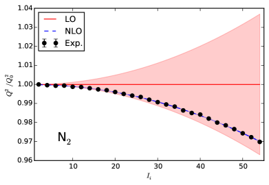
Figure 1: Quadrupole transition moments for decays within the ground band of the N₂ molecule in its para state for states with initial spin $I_{i}$. Experimental data Rothman et al. (2013) (black circles) is compared to LO (red line and corresponding error band) and NLO (blue dashed line and corresponding error band) results of the effective theory. The NLO uncertainty band is very small and barely visible. The quadratic trend (in spin $I_{i}$ of the initial state) at NLO beyond the constant behavior at LO shows the deviation from the rigid rotor.

The much lighter H₂ molecule is farther from the rigid-rotor limit, as shown in Fig. 2. Both, LO and NLO calculations are in agreement with data Rothman et al. (2013). The value $\alpha_{\rm LO}$ is of natural size, while $\alpha_{\rm NLO}\ll 1$, see Table 2. Consequently, the NLO uncertainty is rather small, possibly because the breakdown scale is at a higher energy than naively expected. We note that the N₂ and H₂ molecules beautifully display that deviations of the quadrupole transitions from the rigid-rotor limit are quadratic in the spin of the initial state. This is in accordance with the effective theory. For the molecules, the effective theory is accurate (it describes the data) and precise (theoretical uncertainties are small).

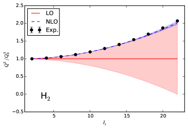
Figure 2: Quadrupole transition moments for decays within the ground band of the H₂ molecule in its para state, for states with initial spin $I_{i}$. Experimental data Rothman et al. (2013) (black circles) is compared to LO (red line and corresponding error band) and NLO (blue dashed line and corresponding error band) results of the effective theory. The quadratic (in spin $I_{i}$ of the initial state) trend at NLO beyond the constant behavior at LO shows the deviation from the rigid rotor.

The last column of Table 1 lists the NLO values for the LECs that enter the quadrupole transition function for the homonuclear molecules. Their values are consistent with the NLO correction $C_{2}/C_{0}^{3}$ obtained from the rotational energy spectrum.

IV.4 Rotational nuclei

Axially-symmetric deformed nuclei possess positive $\mathcal{R}$ parity, and only states with even angular momentum $I$ are allowed in the ground-state band.

The energy spectra of many nuclei in the actinide region makes them good candidates to test the effective theory. Figure 3 shows the quadrupole transition strengths for decays within the ground band of ²³⁶U and compares them to the experimental data from Browne and Tuli (2006). The results from our LO calculations are in good agreement with these data. Unfortunately, the experimental uncertainties are so large that a $\chi^{2}<1$ per datum is already achieved for zero theoretical uncertainties, i.e., for $\alpha_{\rm LO}=0$. The shown theoretical uncertainties are obtained by setting $\alpha_{\rm LO}=1$ for a natural-size estimate. Data of higher precision would be necessary to probe the theory at NLO.

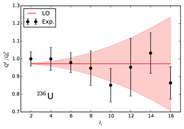
Figure 3: Quadrupole decays within the ground-state band of ²³⁶U for initial spin $I_{i}$. Experimental data Browne and Tuli (2006) with error bars compared to LO calculations of the effective theory. Estimated theoretical uncertainties are shown as bands.

Many rare-earth nuclei are well deformed, and it is interesting to confront the effective theory with data. Figure 4 shows the results for the well-studied nuclei ¹⁶⁶Er McGowan (1981); Fahlander et al. (1992) and ¹⁶²Dy (Hubert et al., 1978; Aprahamian et al., 2006). For ¹⁶⁶Er, a reduced $\chi^{2}<1$ is achieved for zero theoretical uncertainties (see Table 2). Same as with ²³⁶U, the displayed theoretical uncertainties for this nucleus employ $\alpha_{\rm LO}=1$ as a natural-size estimate. For ¹⁶²Dy, the data are consistent with the rigid-rotor result and the error estimates from the effective theory are natural in size. The first deviation only occurs at higher spin, where the experimental uncertainty is increased.

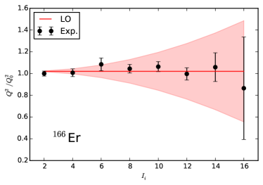
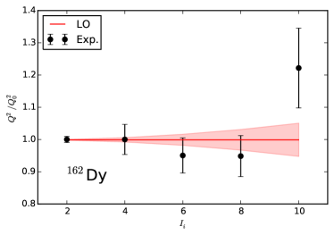
Figure 4: Experimental data (black points with error bars) for decays within the ground band of ¹⁶⁶Er (top) Baglin (2008) and ¹⁶²Dy (bottom) Reich (2007) for initial spin $I_{i}$ is compared to LO results (red line with corresponding uncertainty band) of the effective theory. The data is consistent with the constant LO value of the effective theory and as expected for a rigid rotor.

Results for the well deformed nuclei ¹⁷⁴Yb Browne and Junde (1999), ¹⁶⁸Er Davidson et al. (1981); Warner et al. (1981); McGowan (1981); Kotliński et al. (1990), and ¹⁵⁴Sm are shown in Fig. 5. One of the best rigid-rotor candidates in the rare earth region is ¹⁷⁴Yb due to its small ratio of $\xi/\omega$. Indeed, the breakdown spin is conservatively estimated as $\omega/\xi\approx 19$ from the onset of vibrations and as $\sqrt{C_{0}^{3}/C_{2}}\approx 31$ from the NLO fit to the spectrum (see Table 1). The LO results for this nucleus and our uncertainty estimates are consistent with the experimental data Browne and Junde (1999). We note that the data points for the $4_{g}^{+}\to 2_{g}^{+}$ and the $8_{g}^{+}\to 6_{g}^{+}$ transitions are below and above the rigid-rotor result $Q=Q_{0}$. Within the effective theory, such an oscillatory pattern could only be understood if the breakdown scale were already around spin $I\approx 6$, and this is significantly smaller than expected from the ratios $\omega/\xi$ or $\sqrt{C_{0}^{3}/C_{2}}$ (see Table 1). Thus, higher precision data, particularly for the $6_{g}^{+}\to 4_{g}^{+}$ transition, would be desirable for this nucleus.

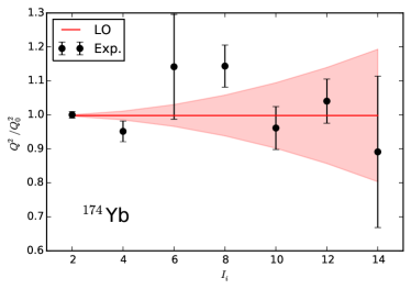
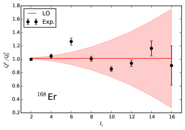
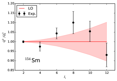
Figure 5: Experimental data (black points with error bars) for decays within the ground band of ¹⁷⁴Yb (top) Browne and Junde (1999), ¹⁶⁸Er (middle) Baglin (2010), ¹⁵⁴Sm (bottom) Reich (2009) for initial spin $I_{i}$ is compared to LO results (red line with corresponding uncertainty band) of the effective theory. With a few notable exceptions the data is largly consistent with the constant LO value of the effective theory and as expected for a rigid rotor. However, the oscillatory pattern of the experimental data is not expected within the effective theory.

For ¹⁶⁸Er the $6_{g}^{+}\to 4_{g}^{+}$ transition is significantly away from the theoretical prediction, and the data exhibit an oscillatory pattern around the rigid-rotor result. This pattern deviates clearly from the effective theory’s expectation of a deviation quadratic in initial spin $I_{i}$ from the rigid-rotor behavior. Within the effective theory, such a behavior could only be understood if the breakdown scale were around the energy of the $6_{g}^{+}$ state, which is unexpectedly low in energy. The relatively large value of $\alpha_{\rm LO}$ in Table 2 also reflects the challenge this nucleus poses. We believe that high-precision measurements, particularly for the $6_{g}^{+}\to 4_{g}^{+}$ transition, would be very interesting for this nucleus.

Finally we turn to ¹⁵⁴Sm. The data is largely consistent with the rigid rotor results expected at LO in the effective theory. Data points fall in the very small interval $0.93Q_{0}^{2}\lesssim Q^{2}\lesssim 1.1Q_{0}^{2}$ around the rigid-rotor prediction. However, taking the relatively small experimental error bars at face value would again suggest that the data oscillates around the constant rigid-rotor value, and this is not expected within the effective theory.

In summary, the data on rotational nuclei is largely consistent with the LO results that describe a rigid rotor. A few transition strengths deviate more than expected from the effective theory, and one would like to see these data points to be measured with a higher precision. In particular, oscillatory patterns around the rigid-rotor results, as displayed by ¹⁷⁴Yb, ¹⁶⁸Er and possibly ¹⁵⁴Sm are unexpected and deserve further attention. The study of subleading corrections, i.e. deviations expected for a non-rigid rotor, would require data with considerably higher precision. It is somewhat surprising that the 1975 words of  Bohr and Mottelson (1975) “The accuracy of the present measurements of $E2$-matrix elements in the ground-state bands of even even nuclei is in most cases barely sufficient to detect deviations from the leading-order intensity relations” are still applicable today. The noted deviations, and the possibility to compare data with more precise predictions for subleading effects, would make it very interesting to measure transition strengths in some of these nuclei with an increased precision.

IV.5 Transitional nuclei

Transitional nuclei are characterized by energy spectra that deviate considerably from the rotational behavior. Ratios $E_{4^{+}}/E_{2^{+}}\approx 3$ identify these non-rigid rotors, and the separation of scale is less pronounced than for the rotational nuclei. The increased $\xi/\omega$ ratio implies that NLO corrections are more relevant and also more visible. Fortunately, for these nuclei data of sufficiently high precision exists. This allows us to check the systematic improvements of the effective theory.

Figure 6 shows data for quadrupole decays in a few transitional nuclei and compares them to theoretical results from the effective theory. For ¹⁸⁸Os (top left panel), the data systematically deviates from the rigid-rotor result and is consistently described at LO and at NLO within the theoretical uncertainties. At spin $I=10$, the theoretical NLO uncertainties exceed the LO uncertainties, signaling the breakdown of the effective theory. This is consistent with the expectation $\sqrt{C_{0}^{3}/C_{2}}\approx 9$ obtained from the fit of the spectrum, see Table 1.

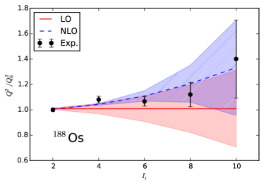
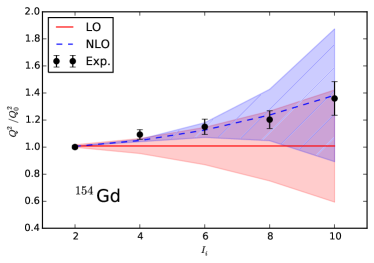
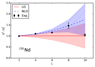
Figure 6: Experimental data (black data points with error bars) for decays within the ground band of ¹⁸⁸Os (top left) Wu et al. (1996), ¹⁵⁴Gd (top right) Tonev et al. (2004), ¹⁵²Sm (bottom left) Zamfir et al. (1999) and ¹⁵⁰Nd (bottom right) Krücken et al. (2002) is compared against LO (red line and corresponding uncertainty band) and NLO (blue dashed line with corresponding uncertainty band) calculations of the effective theory. At NLO, the quadratic deviation (in spin $I_{i}$) from the LO rigid-rotor result is described well by the effective theory.

The quadrupole transitions of the nucleus ¹⁵⁴Gd (top right panel of Fig. 6) agree with expectations for a non-rigid rotor. The quadratic (in $I$) deviations are well described by the theory at NLO. A $\chi^{2}<1$ per datum is obtained at NLO even for vanishing theoretical errors, i.e. for $\alpha_{\rm NLO}=0$ (see Table 2). For the shown NLO error estimates, we set $\alpha_{\rm NLO}=\alpha_{\rm LO}$. This choice is of natural size and consistent with the estimate $\sqrt{C_{0}^{3}/C_{2}}\approx 8$ for the breakdown spin obtained from the fit of the spectrum, see Table 1. The situation is similar for quadrupole transitions in the ground-state band of ¹⁵²Sm (bottom left panel of Fig. 6). Also here, the shown NLO error estimates use $\alpha_{\rm NLO}=\alpha_{\rm LO}$.

Finally, we turn to ¹⁵⁰Nd (bottom right panel of Fig. 6). This nucleus is a non-rigid rotor and well described by the LO and NLO effective theory. The relatively precise value at $I_{i}=10$ deviates from the quadratic deviation expected for a non-rigid rotor but is also in the vicinity of the breakdown scale of the effective theory. Note that the NLO uncertainty band exceeds the LO uncertainty for $I_{i}=10$, and this is consistent with the the estimate $\sqrt{C_{0}^{3}/C_{2}}\approx 7$ for the breakdown spin obtained from the fit of the spectrum, see Table 1.

In summary, the effective theory describes the transitional nuclei rather well. In particular, the quadratic trend (in $I_{i}$) predicted as the NLO correction of the effective theory is demonstrated convincingly. Theoretical uncertainty estimates are consistent as one goes from LO to NLO, and they agree with the precision of the available data. Further progress, e.g the identification of NNLO corrections, would require even more precise data. The existing data suggests that more precise measurements (and possibly the extension to higher spins) could be particularly profitable for ¹⁵⁴Gd and ¹⁵²Sm.

The successful application of the effective theory to the transitional nuclei casts further doubts onto the oscillatory patterns in the experimental data for the rotational ¹⁷⁴Yb and ¹⁶⁸Er, see Fig. 4. As the breakdown scale for rotational nuclei considerably exceeds that for transitional nuclei, one would expect that the effective theory applies even more to the former. This is additional motivation to re-measure more precisely some of the critical transitions in well deformed nuclei.

As we have seen, the effective theory allows us to re-derive some of the well-known results for deformed nuclei Bohr and Mottelson (1975) starting from symmetry principles alone. New elements are the identification of a breakdown scale and its employment in a power counting and in estimates for theoretical uncertainties. In contrast to the phenomenological models – which can be accurate – the effective theory also delivers precision because it can be improved systematically. It is also encouraging that well deformed and transitional nuclei are described on the same footing, without resorting to more special models Iachello (2001) for the latter. For the results presented in this Section, the predictive power of the effective theory equals the traditional approaches Bohr and Mottelson (1975). At LO, one LEC is used to describe the spectrum, and one describes the quadrupole transition strengths. At NLO, one additional LEC each enters the spectrum and the transitions.

V Rotations and vibrations

In this Section, we are interested in inter-band transitions. These transitions are much weaker than the intra-band transitions considered in the previous Section, and the accurate description of these faint transitions poses a challenge. For the description of rotational bands beyond the ground-state band, we need to include additional degrees of freedom into the effective theory. For even-even nuclei, these degrees of freedom represent higher-energetic vibrations of the nucleus with an energy scale $\omega$ below the breakdown energy scale $\Lambda$. These vibrations are the true remnants of Nambu-Goldstone modes in finite systems with emergent symmetry breaking Papenbrock and Weidenmüller (2014). The effective theory for this case has in parts been developed in Refs. Papenbrock (2011); Zhang and Papenbrock (2013). Reference Papenbrock (2011) developed the effective theory up to NLO. In leading order, the theory describes uncoupled vibrational states. At NLO, the vibrational states become heads of rotational bands. Reference Zhang and Papenbrock (2013) focused on higher-order terms. Then, couplings between vibrational band heads enter, and the dependence of the moment of inertia on the quantum numbers of the band heads could be described. In the next Subsection, we briefly introduce quadrupole degrees of freedom. We then develop the Hamiltonian up to NNLO, and finally focus on the coupling of electromagnetic fields for the description of inter-band transitions in the following Section.

V.1 Quadrupole degrees of freedom

In even-even nuclei, the quantized Nambu-Goldstone modes due to the emergent symmetry breaking from SO(3) to SO(2) can be represented by a quadrupole field with two of its components replaced by the low-energy degrees of freedom $\theta$ and $\phi$. Note that these degrees of freedom have the quantum numbers of quadrupole modes, but they are not Bohr’s surface oscillations. In our treatment, the quadrupole degrees of freedom also realize the rotational symmetry nonlinearly; they are in the co-rotating coordinate system and can be viewed as being attached to the particle moving on the two-sphere. We have

$$\Psi=\left(\Psi_{+2},0,\Psi_{0},0,\Psi_{-2}\right).$$ (66)

It is convenient to rewrite the components of the field as

$$\Psi_{0}=\zeta+\psi_{0}\qquad\Psi_{\pm 2}=\psi_{2}e^{\pm i2\gamma}\ .$$ (67)

Here $\zeta$ is the constant vacuum expectation value of the zero mode (with $|\psi_{0}|\ll\zeta$), and the factor 2 in the phase $2\gamma$ has been introduced for convenience. Because of this factor $\gamma$ ranges from $0$ to $\pi$.

The field in the laboratory frame can be written as an appropriate rotation of the field in the intrinsic frame

$$\Phi=g(\phi,\theta)\Psi,$$ (68)

which implies that under the SO(3) rotation $r(\alpha,\beta,\gamma)$

$$\psi_{0}\rightarrow\psi_{0}\qquad\psi_{2}\rightarrow\psi_{2}\qquad\gamma\rightarrow\gamma+\chi.$$ (69)

Here, $\chi=\chi(\alpha,\beta,\gamma;\theta,\phi)$ is a complicated function of the rotation angles and the orientation angles $(\theta,\phi)$; the rotational symmetry is realized nonlinearly Papenbrock (2011).

The kinetic terms in the quadrupole degrees of freedom are obtained by acting with the covariant derivative (5) onto $\Psi$. Thus, any Lagrangian $L$ in $v_{\pm}$, $\Psi_{0}$, $\Psi_{\pm 2}$, $D_{t}\Psi_{0}$, $D_{t}\Psi_{\pm 2}$ that is formally invariant under SO(2), is invariant under SO(3) due to the nonlinear realization of the rotational symmetry. The application of Noether’s theorem to such Lagrangian yields the total angular momentum $\mathbf{J}$ with spherical components

$$\begin{split}J_{+1}&=-{1\over\sqrt{2}}e^{i\phi}(ip_{\theta}-p_{\phi}\cot{\theta})-{\frac{1}{\sqrt{2}}}e^{i\phi}\frac{p_{\gamma}}{\sin{\theta}}\\ J_{0}&=p_{\phi}\\ J_{-1}&=-{1\over\sqrt{2}}e^{-i\phi}(ip_{\theta}+p_{\phi}\cot{\theta})+\frac{1}{\sqrt{2}}e^{-i\phi}\frac{p_{\gamma}}{\sin{\theta}},\end{split}$$ (70)

as the conserved quantity. Here

$$p_{\theta}\equiv\partial_{\dot{\theta}}L\qquad p_{\phi}\equiv\partial_{\dot{\phi}}L\qquad p_{\gamma}\equiv\partial_{\dot{\gamma}}L,$$ (71)

and the total angular momentum squared is

$$\mathbf{J}^{2}=p_{\theta}^{2}+\left(\frac{p_{\phi}-p_{\gamma}\cos{\theta}}{\sin{\theta}}\right)^{2}+p_{\gamma}^{2}.$$ (72)

We denote the total angular momentum as $\mathbf{J}$, because its definition (70) differs from Eq. (6) due to the newly introduced vibrational degrees of freedom.

Let us briefly compare the degrees of freedom in the effective theory to those of the Bohr Hamiltonian. In the effective theory, the angles $(\phi,\theta,\gamma)$ can be viewed as Euler angles, with the “slow” degrees of freedom $\Omega=(\theta,\phi)$ describing the orientation of the symmetry axis and the “fast” degree of freedom $\gamma$ describing rotations around the symmetry axis. The $\psi_{0}$ degree of freedom is a (fast) vibration that keeps the axial symmetry, while $\psi_{2}$ is a (fast) vibration that breaks the axial symmetry. The Bohr Hamiltonian employs three Euler angles and two deformation parameters Próchniak and Rohoziński (2009). The two deformation parameters (usually labeled as $\beta$ and $\gamma$, respectively) describe the amplitude of the total deformations ($\beta$), and the deformation breaks axial symmetry for $\gamma\neq 0$. The variable $\beta$ can be viewed as a hyper radius in five-dimensional space of the quadrupole degrees of freedom, while $\gamma$ is a hyper angle in addition to the three Euler angles.

V.2 Power counting and Hamiltonian at NNLO

In addition to the power counting estimates (10) we have Papenbrock (2011)

$$\begin{split}\omega_{0}\sim\omega_{2}\sim\dot{\gamma}\sim\omega&\qquad\dot{\psi_{0}}\sim\dot{\psi_{2}}\sim\omega^{1/2}\\ \zeta\sim\xi^{-1/2}&\qquad\psi_{0}\sim\psi_{2}\sim\omega^{-1/2}.\end{split}$$ (73)

For an understanding of this scaling we recall that the angles $\theta$, $\phi$ and $\gamma$ are dimensionless, and that a time derivative on these degrees of freedom must scale as the excitation energy of the motion they generate. The scaling of $\psi_{i}$, $i=0,2$, is such that $\dot{\psi_{i}}^{2}\sim\omega$. The expectation value $\zeta$ is associated with the emergent symmetry breaking and must scale as $\xi^{-1/2}$.

The Lagrangian of this effective theory is $L_{\rm LO}+L_{\rm NLO}+L_{\rm NNLO}$ where the leading-order Lagrangian

$$L_{\rm LO}=\frac{1}{2}\dot{\psi}_{0}^{2}+\dot{\psi}_{2}^{2}+4\dot{\gamma}^{2}\psi_{2}^{2}-\frac{\omega_{0}^{2}}{2}\psi_{0}^{2}-\frac{\omega_{2}^{2}}{4}\psi_{2}^{2}$$ (74)

describes vibrations at the high-energy scale $\omega$, the NLO correction

$$L_{\rm NLO}=\frac{C_{0}}{2}\left(\dot{\theta}^{2}+\dot{\phi}^{2}\sin^{2}{\theta}\right)+4\psi_{2}^{2}\dot{\gamma}\dot{\phi}\cos{\theta}$$ (75)

couples rotations at the low-energy scale $\xi$ to vibrations via the $\gamma$ degree of freedom, and the NNLO correction

$$\begin{split}L_{\rm NNLO}&=\frac{C_{\beta}}{2}\psi_{0}\left(\dot{\theta}^{2}+\dot{\phi}^{2}\sin^{2}{\theta}\right)\\ &+\frac{C_{\gamma}}{2}\psi_{2}\left(\dot{\theta}^{2}-\dot{\phi}^{2}\sin^{2}{\theta}\right)\cos{2\gamma}\\ &+C_{\gamma}\psi_{2}\dot{\theta}\dot{\phi}\sin{2\gamma}\sin{\theta},\end{split}$$ (76)

is treated as a perturbation that scales as $\xi(\xi/\omega)^{1/2}$. According to the power counting 73, this implies

$$C_{\beta}\sim C_{\gamma}\sim\xi^{-1/2}.$$ (77)

Note that $\gamma$ is a cyclic variable of the LO and NLO Lagrangians. Thus, at these orders, the projection of the angular momentum $\mathbf{J}$ onto the intrinsic symmetry axis $p_{\gamma}$, is a conserved quantity in addition to the total angular momentum (70).

A Legendre transformation of the Lagrangian yields the Hamiltonian $H_{\rm LO}+H_{\rm NLO}+H_{\rm NNLO}$. Here

$$H_{\rm LO}=\frac{p_{0}^{2}}{2}+\frac{\omega_{0}^{2}}{2}\psi_{0}^{2}+\frac{p_{2}^{2}}{4}+\frac{1}{4\psi_{2}^{2}}\left(\frac{p_{\gamma}}{2}\right)^{2}+\frac{\omega_{2}^{2}}{4}\psi_{2}^{2}$$ (78)

is the Hamiltonian of a harmonic oscillator with frequency $\omega_{0}$ coupled to a two-dimensional harmonic oscillator with frequency $\omega_{2}$. The quantization is standard

$$\hat{p}_{0}=-i\partial_{\psi_{0}}\qquad\hat{p}_{2}=-i\partial_{\psi_{2}}\qquad\hat{p}_{\gamma}=-i\partial_{\gamma}.$$ (79)

We denote the eigenstates of the LO Hamiltonian as $|n_{0}n_{2}K/2\rangle$, with integer $n_{0}$ and $n_{2}$ and even $K$. Here $n_{0}$, $n_{2}$ and $K/2$ are the number of quanta of the modes $\psi_{0}$, $\psi_{2}$, and $\gamma$, respectively. These states can be written as $|n_{0}\rangle|n_{2}\rangle|K/2\rangle$, where $|n_{0}\rangle$ are the states of the harmonic oscillator, and $\langle\psi_{2}|n_{2}\rangle$ are the radial wave functions of the two-dimensional harmonic oscillator.

The NLO correction

$$H_{\rm NLO}=\frac{1}{2C_{0}}\mathbf{p}_{\Omega\gamma}^{2}=\frac{1}{2C_{0}}\left(\mathbf{J}^{2}-p_{\gamma}^{2}\right)$$ (80)

is the Hamiltonian of a symmetric top Merzbacher (1961). Here, the momentum in the tangential plane is

$$\mathbf{p}_{\Omega\gamma}=\mathbf{e}_{\theta}p_{\theta}+\mathbf{e}_{\phi}p_{\phi\gamma},$$ (81)

with

$$p_{\phi\gamma}\equiv\frac{p_{\phi}-p_{\gamma}\cos{\theta}}{\sin{\theta}}.$$ (82)

We also have

$$\mathbf{J}=\mathbf{e}_{r}\times\mathbf{p}_{\Omega\gamma}+\mathbf{e}_{r}p_{\gamma}\ .$$ (83)

This form of the angular momentum agrees with the intuition. In particular, rotations around the symmetry axis $\mathbf{e}_{r}$ yield a contribution to the angular momentum in the direction of this axis.

The quantization

$$\begin{split}\hat{\mathbf{p}}_{\Omega\gamma}&=-i\mathbf{e}_{\theta}\partial_{\theta}-i\mathbf{e}_{\phi}\frac{\partial_{\phi}-\partial_{\gamma}\cos{\theta}}{\sin{\theta}}\\ &=-\mathbf{e}_{r}\times\hat{\mathbf{J}}\end{split}$$ (84)

is standard. In what follows, we denote the differential operator corresponding to the momentum operator $\hat{\mathbf{p}}_{\Omega\gamma}$ also as

$$-i\mathbf{\nabla}_{\Omega\gamma}\equiv\mathbf{p}_{\Omega\gamma}.$$ (85)

The Hamiltonian eigenvalue problem becomes

$$\hat{H}_{\rm NLO}|IMK\rangle=\frac{1}{2C_{0}}\left[I(I+1)-K^{2}\right]|IMK\rangle.$$ (86)

Here, we continued to denote the eigenvalues of the total angular momentum by the quantum number $I$. The wave functions are linear combinations of Wigner $D$ functions, consistent with the positive $\mathcal{R}$ parity of the system, i.e.

$$\langle\Omega\gamma|IMK\rangle=N\left[D_{MK}^{I}(\Omega,\gamma)+(-1)^{I}D_{M-K}^{I}(\Omega,\gamma)\right].$$ (87)

Here $N$ is a normalization factor. For $K=0$, the wave function cannot take odd $I$ values due to the $\mathcal{R}$ parity. Thus, for even $I$ the wave function takes the form

$$\langle\Omega\gamma|IM0\rangle=\sqrt{\frac{2I+1}{4\pi^{2}}}D_{M0}^{I}(\Omega,\gamma)=\frac{(-1)^{m}}{\sqrt{\pi}}Y_{I-M}(\Omega).$$ (88)

The Wigner D-functions $D_{MK}^{I}(\Omega\gamma)$ fulfill the relations Varshalovich et al. (1988)

$$\begin{split}\hat{J}_{z}D_{MK}^{J}(\Omega\gamma)&=-MD_{MK}^{I}(\Omega\gamma)\\ \hat{J}_{z^{\prime}}D_{MK}^{J}(\Omega\gamma)&=-KD_{MK}^{I}(\Omega\gamma)\\ \hat{\mathbf{J}}^{2}D_{MK}^{J}(\Omega\gamma)&=I(I+1)D_{MK}^{I}(\Omega\gamma).\end{split}$$ (89)

The complete Hamiltonian at NLO can be diagonalized as

$$\left(\hat{H}_{\rm LO}+\hat{H}_{\rm NLO}\right)|n_{0}n_{2}IMK\rangle=\bigg{[}\omega_{0}\left(n_{0}+\frac{1}{2}\right)$$

$$+{\omega_{2}\over 2}\left(2n_{2}+\frac{K}{2}+1\right)+\frac{I(I+1)-K^{2}}{2C_{0}}\bigg{]}|n_{0}n_{2}IMK\rangle.$$

Thus, at this order, the spectrum consists of rotational bands with rotational constant $1/(2C_{0})$ on top of harmonic vibrations. The vibrational quanta determine the band head, and the ground-state band has no vibrational quanta excited. Because $0\leq\gamma\leq\pi$, the wave function in $\gamma$ must exhibit periodic boundary conditions at the domain boundaries. This limits $K$ to even values. Historically, the band head with $(n_{0}=1,n_{2}=0,K=0)$, and the band head with $(n_{0}=0,n_{2}=0,K=2)$ determine the “$\beta$ band” and the “$\gamma$ band” respectively. In what follows, we continue to use these labels.

The NNLO correction to the Hamiltonian is

$$H_{\rm NNLO}=-\frac{1}{2C_{0}^{2}}\left(C_{\beta}\psi_{0}\mathbf{p}_{\Omega\gamma}^{2}+C_{\gamma}\psi_{2}\mathbf{p}_{\Omega\gamma}^{T}\hat{\Gamma}\mathbf{p}_{\Omega\gamma}\right).$$ (91)

Here,

$$\hat{\Gamma}\equiv\left[\begin{array}[]{c c}\cos{2\gamma}&\sin{2\gamma}\\ \sin{2\gamma}&-\cos{2\gamma}\\ \end{array}\right]$$ (92)

acts on vectors in the tangent plane. The operator $\hat{H}_{\rm NNLO}$ is off-diagonal in the eigenstates of the NLO Hamiltonian. Thus, it is only effective in second-order perturbation theory, i.e. at order N³LO. At that order, corrections to the rotational constant (or the effective moment of inertia) linear in the number of excited quanta are introduced Zhang and Papenbrock (2013). These corrections arise due to omitted physics at the breakdown scale $\Lambda\sim 3$ MeV, where pair-breaking effects need to be taken into account Papenbrock and Weidenmüller (2014). Thus, deviations from the harmonic behavior of the band heads is expected to scale as $\omega/\Lambda\approx 1/3$ for nuclei in the rare-earth and actinide regions. In the following Section, we will determine the LECs $C_{\beta}$ and $C_{\gamma}$ by fit to inter-band transitions. In the long run, it would be interesting to compute LECs from more microscopic methods Caprio et al. (2013); Dytrych et al. (2013).

VI Inter-band transitions

In this Section, we couple electromagnetic fields to the Hamiltonian, and focus on the inter-band transitions. These transitions are much fainter than the strong intra-band transitions discussed in the Sect. IV. The transitions from the $\beta$ band to the ground-state band are not understood very well (see Ref. Garrett (2001) for a review), because the traditional models overpredict them by up to an order of magnitude. Furthermore, these transitions vary by about two orders of magnitude in well-deformed and transitional nuclei Aprahamian (2004). Below we will see that the transitions pose no challenge to the effective theory. For the LO description of these transitions, we only need to gauge the NNLO Hamiltonian.

VI.1 Transition operators

The NNLO Hamiltonian of the previous section can be coupled to an electromagnetic field employing the gauging

$$\hat{\mathbf{p}}_{\Omega\gamma}\rightarrow\hat{\mathbf{p}}_{\Omega\gamma}-q\mathbf{A}_{\Omega}=-i\nabla_{\Omega\gamma}-q\mathbf{A}_{\Omega}\ .$$ (93)

This is equivalent to

$$\mathbf{J}\to\mathbf{J}-q\mathbf{e}_{r}\times\mathbf{A}_{\Omega}\ ,$$ (94)

and in full analogy to Eq. (37).

Thus, the angles $\theta$, $\phi$, and $\gamma$ are gauged. Assuming that the vibrational degrees of freedom $\psi_{0}$ and $\psi_{2}$ also carry a charge, we could also couple these to the radial component $\mathbf{A}\cdot\mathbf{e}_{r}$ to obtain a rotationally invariant and gauge-invariant Hamiltonian. As discussed below, the corresponding terms do not yield independent contributions for the intra-band transitions considered in this paper, and they are therefore neglected.

The gauging of the NNLO contribution (91) to the Hamiltonian

$$\hat{H}_{\rm NNLO}^{(\mathbf{A})} = \frac{iq}{2C_{0}}\frac{C_{\beta}}{C_{0}}\psi_{0}\left(\mathbf{A}\cdot\nabla_{\Omega\gamma}+\nabla_{\Omega\gamma}\cdot\mathbf{A}\right)$$ (95)

$$+ \frac{iq}{2C_{0}}\frac{C_{\gamma}}{C_{0}}\psi_{2}\left(\mathbf{A}^{T}\hat{\Gamma}\nabla_{\Omega\gamma}+\nabla_{\Omega\gamma}^{T}\hat{\Gamma}\mathbf{A}\right)$$

induces LO inter-band transitions. As the inter-band transitions originate from a small correction to the Hamiltonian, they are expected to be an order of magnitude weaker (in the power counting) than the intra-band transitions. Gauging of the fields $\psi_{0}$ and $\psi_{2}$ would add terms $q_{0}A_{r}\hat{p}_{0}$ and $q_{2}A_{r}\hat{p}_{2}$ to the Hamiltonian. Here $A_{r}=\mathbf{A}\cdot\mathbf{e}_{r}$. These operators do not yield transition matrix elements that differ from those of the operators in the Hamiltonian (95). They are therefor neglected.

Following Eq. (55) we compute the transition strength as

$$B(E\lambda,i\rightarrow f)=\frac{1}{2l_{i}+1}\left|\langle f||\mathscr{M}(E\lambda)||i\rangle\right|^{2}\ .$$ (96)

where $\hat{\mathscr{M}}(E\lambda)\equiv\hat{H}^{(\mathbf{A}^{(\lambda)})}/(wA)$, $w\equiv[I_{f}(I_{f}+1)-I_{i}(I_{i}+1)+K_{i}^{2}]/2C_{0}$, and $k$ is the energy (or momentum) of the photon involved in the transition.

The LO inter-band $B(E2)$ values for transitions from the $\beta$ band to the ground band are

$$B(E2,i_{\beta}\rightarrow f_{g})=\frac{C_{\beta}^{2}}{2C_{0}^{2}\omega_{0}}\frac{q^{2}}{60}\left(C_{I_{i}020}^{I_{f}0}\right)^{2},$$ (97)

while LO $B(E2)$ values for transitions from the $\gamma$ band to the ground band are

$$B(E2,i_{\gamma}\rightarrow f_{g})=\frac{3C_{\gamma}^{2}}{2C_{0}^{2}\omega_{2}}\frac{q^{2}}{60}\left(C_{I_{i}22-2}^{I_{f}0}\right)^{2}.$$ (98)

We can generalize the definition of the quadrupole transition moments to

$$Q_{if}^{2}=\frac{B(E2,i\rightarrow f)}{\left(C_{I_{i}K_{i}2K_{f}-K_{i}}^{I_{f}K_{f}}\right)^{2}}\ ,$$ (99)

then

$$Q_{i_{\beta}f_{g}}^{2}=\frac{C_{\beta}^{2}}{2C_{0}^{2}\omega_{0}}Q^{2}\ ,\qquad Q_{i_{\gamma}f_{g}}^{2}=\frac{3C_{\gamma}^{2}}{2C_{0}^{2}\omega_{2}}Q^{2},$$ (100)

where $Q\equiv\sqrt{q^{2}/60}$. We note that the strengths of transitions from the $\beta$ band are similar to those of the $\gamma$ band for similarly sized LECs $C_{\beta}$ and $C_{\gamma}$.

We note that – within the effective theory – the intra-band transitions depend on the LECs $C_{\beta}$ and $C_{\gamma}$. We recall that these LECs enter at the Hamiltonian at NNLO as off-diagonal corrections to the Hamiltonian, which prevents us from adjusting them to spectra at this order. As more terms enter the Hamiltonian at N³LO, it seems attractive to determine $C_{\beta}$ and $C_{\gamma}$ instead by inter-band transitions. In what follows, we adjust these coefficients to the description of one inter-band transition from the respective band to the ground band. Other inter-band transitions then are predictions.

In the traditional collective models, no new parameters enter the computation of the inter-band transitions. As a result, these faint transitions are overpredicted substantially. For example, the inter-band $B(E2)$ values according to the adiabatic Bohr model are (See, e.g., Ref. Rowe and Wood (2010))

$$B(E2,i_{\beta}\to f_{g}) = \frac{\xi}{2\omega_{0}}\left(\frac{Ze\beta_{0}}{A}\right)^{2}\left(C_{l_{i}020}^{l_{f}0}\right)^{2}\$$

$$B(E2,i_{\gamma}\to f_{g}) = \frac{2\xi}{\omega_{2}}\left(\frac{Ze\beta_{0}}{A}\right)^{2}\left(C_{l_{i}22-2}^{l_{f}0}\right)^{2},$$ (101)

implying inter-band transitions from the $\beta$ are only a factor two weaker than those from the $\gamma$ bands. Here, $\beta_{0}$ is a deformation parameter. Thus, the effective theory is richer in structure (through two additional parameters). This more complex structure is a consequence of a theory that is based on symmetry principles alone. It will allow us to describe inter-band transitions much more accurately. Regarding ratios of inter-band transition strengths, the effective theory at leading order reproduces the traditional collective models as expected from the Alaga rules.

VI.2 Comparison with experimental data

We test the expressions (97) and (98) by confronting them to data for inter-band transitions in ^166,168Er and ¹⁵⁴Sm. These isotopes of erbium are considered good rotors, while the samarium isotope is between rotors and transitional nuclei.

For ¹⁶⁸Er, the relevant energies are $\xi\approx 79.8$ keV, $\omega_{0}\approx 1217.2$ keV, and $\omega_{2}/2\approx 821.2$ keV. In the spirit of the theory, all constants were fitted to low-energy data. Thus, the effective quadrupole moment was fitted via the $2_{g}^{+}\to 0_{g}^{+}$ transition, while the values $C_{\beta}\approx 0.077$ keV^-1/2 and $C_{\gamma}\approx 0.203$ keV^-1/2 are determined from the $2_{\beta}^{+}\to 0_{g}^{+}$ and $2_{\gamma}^{+}\to 2_{g}^{+}$ transitions, respectively. We employed data from Ref. Baglin (2010) and Ref. Kotliński et al. (1990) for completion. The values of these LECs are natural in size when compared to the scale $\xi^{-1/2}\approx 0.112$ keV^-1/2. Clearly, more precise data for transitions between the $\beta$ and ground bands is required to determine the size of $C_{\beta}$. All other transitions are predictions. Table 3 shows experimental and theoretical $B(E2)$ values for transitions within the ground-state band and inter-band transitions in ¹⁶⁸Er. Overall, the effective theory describes the data well. The theoretical uncertainties presented in Table 3 for transitions in the ground-state band are based on the discussion in Subsection IV.2. However, for the uncertainties of transitions from the $\beta$ band or the $\gamma$ band, we employed more conservative uncertainty estimates based on the larger ratio $(\omega/\Lambda)^{2}\approx 0.25$ that is due to the proximity of the breakdown scale $\Lambda$.

Table 3: Transition strength for ¹⁶⁸Er in units of e²b². Experimental transitions strengths $B(E2)_{\rm exp}$ are compared to theoretical results $B(E2)_{\rm ET}$ from the effective theory and $B(E2)_{\rm BH}$ from the adiabatic Bohr Hamiltonian. Experimental values are taken from Baglin (2010) unless otherwise specified. Values for the adiabatic Bohr Hamiltonian are taken from Rowe and Wood (2010). Parenthesis denote experimental errors and theoretical uncertainty estimates.

$i\rightarrow f$	$B(E2)_{\rm exp}$	$B(E2)_{\rm ET}$	$B(E2)_{\rm BH}$
$2_{g}^{+}\rightarrow 0_{g}^{+}$	$1.173(22)$	$1.173$	$1.173$
$4_{g}^{+}\rightarrow 2_{g}^{+}$	$1.756(50)$	$1.676(36)$	$1.677$
$6_{g}^{+}\rightarrow 4_{g}^{+}$	$2.335(99)$	$1.846(91)$	$1.842$
$8_{g}^{+}\rightarrow 6_{g}^{+}$	$1.949(72)$	$1.932(169)$	$1.935$
$2_{\gamma}^{+}\rightarrow 0_{g}^{+}$	$0.0258(9)$	$0.0309(77)$	$0.1126$
$2_{\gamma}^{+}\rightarrow 2_{g}^{+}$	$0.0442(38)$	$0.0442$	$0.1610$
$2_{\gamma}^{+}\rightarrow 4_{g}^{+}$	$0.0034(2)$	$0.0022(5)$	$0.0080$
$2_{\beta}^{+}\rightarrow 0_{g}^{+}$	$0.0020(^{+8}_{-20})$	$0.0020$	$0.0387$
$2_{\beta}^{+}\rightarrow 2_{g}^{+}$		$0.0029(7)$	$0.0553$
$2_{\beta}^{+}\rightarrow 4_{g}^{+}$	$0.0121(^{+44}_{-121})$	$0.0051(13)$	$0.0995$

For ¹⁶⁶Er, the energy scales are $\xi\approx 80.6$ keV, $\omega_{0}\approx 1460$ keV and $\omega_{2}/2\approx 785.9$ keV. This yields $C_{\beta}\approx 0.111$ keV^-1/2 and $C_{\gamma}\approx 0.213$ keV^-1/2, and both values are natural in size when compared to $\xi^{-1/2}\approx 0.111$ keV^-1/2. Once again, more precise experimental $B(E2)$ values for transitions between the $\beta$ and ground bands would be valuable. Table 4 shows experimental and theoretical $B(E2)$ values for intra-band and inter-band transitions in this nucleus. Theoretical uncertainties are given as discussed for ${168}$Er. The experimental $B(E2)$ value for the $2_{\beta}^{+}\to 4_{g}^{+}$ transition is too large (one order of magnitude larger than decays from the $\gamma$ band to the ground band) to be understood within the effective theory.

Table 4: Same as Table 3 but for ¹⁶⁶Er. Experimental values are taken from Baglin (2008).

$i\rightarrow f$	$B(E2)_{\rm exp}$	$B(E2)_{\rm ET}$	$B(E2)_{\rm BH}$
$2_{g}^{+}\rightarrow 0_{g}^{+}$	$1.175(27)$	$1.175$	$1.175$
$4_{g}^{+}\rightarrow 2_{g}^{+}$	$1.718(61)$	$1.679(24)$	$1.680$
$6_{g}^{+}\rightarrow 4_{g}^{+}$	$2.037(110)$	$1.849(60)$	$1.845$
$8_{g}^{+}\rightarrow 6_{g}^{+}$	$2.054(77)$	$1.935(112)$	$1.939$
$2_{\gamma}^{+}\rightarrow 0_{g}^{+}$	$0.0285(12)$	$0.0370(93)$	$0.1205$
$2_{\gamma}^{+}\rightarrow 2_{g}^{+}$	$0.0529(33)$	$0.0529$	$0.1721$
$2_{\gamma}^{+}\rightarrow 4_{g}^{+}$	$0.0043(2)$	$0.0026(7)$	$0.0086$
$2_{\beta}^{+}\rightarrow 0_{g}^{+}$	$0.0036(4)$	$0.0036$	$0.0324$
$2_{\beta}^{+}\rightarrow 2_{g}^{+}$		$0.0051(13)$	$0.0463$
$2_{\beta}^{+}\rightarrow 4_{g}^{+}$	$0.2113(325)$	$0.0093(23)$	$0.0834$

Let us also attempt to describe a non-rigid rotor. The region around ¹⁵²Sm has been well studied Zamfir et al. (1999); Casten and Zamfir (2001); Garrett et al. (2009), and absolute $B(E2)$ values for some inter-band transitions in ¹⁵⁴Sm were measured recently Möller et al. (2012). For ¹⁵⁴Sm, the LECs related to inter-band transitions are $C_{\beta}\approx 0.092$ keV^-1/2 (determined from the $2_{\beta}^{+}\to 2_{g}^{+}$ transition) and $C_{\gamma}\approx 0.181$ keV^-1/2. Both values are natural in size when compared to $\xi^{-1/2}\approx 0.110$ keV^-1/2. Table 5 shows our LO results for this nucleus. The theoretical uncertainties are computed as discussed for ¹⁶⁸Er. We also show theoretical results of the confined $\beta$ soft (CBS) model Pietralla and Gorbachenko (2004), as an example that a particular model can approximately account for the magnitude of some of the transitions between the $\beta$ band and the ground-state band.

Table 5: Same as Table 3 but for ¹⁵⁴Sm. Theoretical results from the confined $\beta$ soft (CBS) model Pietralla and Gorbachenko (2004), taken from Ref. Möller et al. (2012), are also included. Experimental values are taken from Reich (2009) and Möller et al. (2012) for intra-band and inter-band transitions, respectively.

$i\rightarrow f$	$B(E2)_{\rm exp}$	$B(E2)_{\rm ET}$	$B(E2)_{\rm CBS}$	$B(E2)_{\rm BH}$
$2_{g}^{+}\rightarrow 0_{g}^{+}$	$0.863(5)$	$0.863$	$0.853$	$0.863$
$4_{g}^{+}\rightarrow 2_{g}^{+}$	$1.201(29)$	$1.233(9)$	$1.231$	$1.234$
$6_{g}^{+}\rightarrow 4_{g}^{+}$	$1.417(39)$	$1.358(23)$	$1.378$	$1.355$
$8_{g}^{+}\rightarrow 6_{g}^{+}$	$1.564(83)$	$1.421(43)$	$1.471$	$1.424$
$2_{\gamma}^{+}\rightarrow 0_{g}^{+}$	$0.0093(10)$	$0.0110(28)$		$0.0492$
$2_{\gamma}^{+}\rightarrow 2_{g}^{+}$	$0.0157(15)$	$0.0157$		$0.0703$
$2_{\gamma}^{+}\rightarrow 4_{g}^{+}$	$0.0018(2)$	$0.0008(2)$		$0.0050$
$2_{\beta}^{+}\rightarrow 0_{g}^{+}$	$0.0016(2)$	$0.0025(6)$	$0.0024$	$0.0319$
$2_{\beta}^{+}\rightarrow 2_{g}^{+}$	$0.0035(4)$	$0.0035$	$0.0069$	$0.0456$
$2_{\beta}^{+}\rightarrow 4_{g}^{+}$	$0.0065(7)$	$0.0063(16)$	$0.0348$	$0.0821$

We note that the ratio $C_{\gamma}/C_{\beta}$, while usually natural in size, fulfills $C_{\gamma}/C_{\beta}>1$ for the nuclei we just considered. As the LECs $C_{\beta}$ and $C_{\gamma}$ enter quadratically into $B(E2)$ transition strengths, the transitions from the $\beta$ band to the ground-state band are considerably weaker than the transitions from the $\gamma$ band to the ground-state band.

The most important result of this paper is that the effective theory, with its model-independent approach to the collective Hamiltonian and its corresponding transition operators, suggests a step toward the solution of the long-standing problem posed by the faint inter-band transitions. The consistent description of Hamiltonian and currents shows that the observed strengths of inter-band transitions can be described within the effective theory using LECs of natural size. As a consequence, the strengths of the interband $E2$ transitions are also natural in size. From this perspective it seems adequate to keep referring to the $0_{2}^{+}$ rotational band as the $\beta$ band. The effective theory predicts the strength of inter-band transitions once a single transition determines a LEC of the Hamiltonian.

Let us finally also comment on NLO corrections to inter-band transitions. These corrections are beyond the scope of the present paper. Recently, Kulp et al. (2006) precisely measured ratios of transitions intensities between the $\gamma$ band and the ground-state band in ¹⁶⁶Er. They confirmed the beyond-leading-order predictions by Mikhailov (1966) to a high level of accuracy.

VII Discussion

The geometric collective models approach low-lying excitations in deformed nuclei as quantized surface oscillations of a liquid drop. In contrast, the effective theory for deformed nuclei assumes symmetry properties (such as rotational invariance), the emergent breaking of rotational symmetry (and the ensuing separation of scales), and the existence of a breakdown scale. It then builds the most general Hamiltonian (and currents) consistent with these assumptions and orders them in magnitude based on the power counting. Not surprisingly, the effective theory – particularly beyond leading order – has more parameters than the traditional models. The geometrical models quantitatively predict several aspects of deformed nuclei, e.g. rotational bands with similar-sized rotational constants on top of intrinsic vibrations together with strong in-band transitions. The effective theory obtains these results in leading and subleading order.

Other aspects, such as the small variation of rotational constants with the quantum numbers of the band heads, or the magnitude of inter-band transitions are not described quantitatively correct by the tradtional models. In contrast, the effective theory also captures these finer details, as shown for the rotational constants in Ref. Zhang and Papenbrock (2013) and for the inter-band transitions in this work. This suggests that the assumptions made by the models are correct only to a certain order. The effective theory’s capability in accounting also for the finer details suggest that its underlying assumptions are sound. The effective theory delivers increased precision (with consistent uncertainty estimates) at the expense of additional parameters. This can be useful if correspondingly precise data is available, which is the case for in-band transitions in transitional nuclei and for inter-band transitions considered in this work. This aspect is also of interest with view on the advent of powerful $\gamma$-ray detectors Paschalis et al. (2013).

The capability to estimate theoretical uncertainties is essential when confronting theory and experiment. It is natural to effective theories because of their power counting. In addition, the identification of a breakdown scale makes clear up to which energies the theory can be applied. We believe Figs. 4 and 5 would carry little information without the theoretical uncertainty estimates. These estimates motivate us to propose re-measurements or re-evaluations of certain data.

VIII Summary

We studied $E2$ transitions in deformed nuclei within a model-independent approach based on an effective theory. The effective theory is based on the emergent symmetry breaking of rotational symmetry to axial symmetry. Electromagnetic transitions result from gauging of the Hamiltonian, and from higher-order non-minimal couplings that are consistent with gauge invariance and the symmetry of the system under consideration. The estimate of theoretical uncertainties is one of the highlights of the effective theory approach.

Homonuclear molecules provide us with an ideal test case because they possess a very large separation of scale and therefore exhibit only small corrections to the rigid-rotor limit. The effective theory describes $E2$ transitions in the diatomic molecules N₂ and H₂ very well, and deviations are within the theoretical uncertainties.

The effective theory describes $B(E2)$ transitions in the ground-state bands of well-deformed nuclei at leading order, and more precise experimental data are necessary to probe subleading effects. Our model-independent results also suggest that some low-lying transitions in these nuclei would probably merit a more precise re-measurement or re-evaluation of data, because they can not be easily understood within the effective theory. For transitional nuclei, the existing data are sufficiently precise to probe the effective theory at subleading oder. Here, data and theoretical results are consistent within theoretical uncertainties.

For $E2$ transitions within ground-state bands, the effective theory reproduces known results of the Bohr Hamiltonian. The employment of the beakdown scale and the power counting allows us to estimate theoretical uncertainties and to meaningfully confront data. A somewhat surprising result is that well-deformed nuclei do not challenge theory because of insufficient precision of the available data.

The effective theory also suggests that the electromagnetic structure of deformed nuclei is more complex than the collective models assume, regarding both the Hamiltonian and the transition operator. The magnitude of the faint inter-band transitions is captured correctly within the effective theory, thus addressing to a long-standing problem. In the effective theory, this comes at the expense of new parameters, and one needs to know a single inter-band transition strength to make leading-order predictions for other transitions between the bands in question. These results also cast some doubt on the traditional usage of the quadrupole operator to describe faint electromagnetic transitions, as this approach seems to be limited to the strong (leading order) transitions between states within a band.

This work shows that the effective theory for deformed nuclei reproduces the traditional collective models regarding leading-order aspects (spectra and transitions) of deformed nuclei. In contrast to the models, however, the effective theory also accounts for finer details, and it provides us with theoretical error estimates. We would hope that the results presented in this work might stimulate more precise measurements of electromagnetic transitions in deformed nuclei.