Analysis of a two-level algorithm for HDG methods for diffusion problems

Abstract

This paper analyzes an abstract two-level algorithm for hybridizable discontinuous Galerkin (HDG) methods in a unified fashion. We use an extended version of the Xu-Zikatanov (X-Z) identity to derive a sharp estimate of the convergence rate of the algorithm, and show that the theoretical results also apply to weak Galerkin (WG) methods. The main features of our analysis are twofold: one is that we only need the minimal regularity of the model problem; the other is that we do not require the triangulations to be quasi-uniform. Numerical experiments are provided to confirm the theoretical results.
Keywords. two-level algorithm, hybridizable discontinuous Galerkin method, weak Galerkin method, multigrid, X-Z identity

1 Introduction

The Hybridizable Discontinuous Galerkin (HDG) framework, proposed in [17] (2009) for second order elliptic problems, provides a unifying strategy for hybridization of finite element methods. The unifying framework includes as particular cases hybridized versions of mixed methods [2, 7, 13], the continuous Galerkin (CG) method [15], and a wide class of hybridizable discontinuous Galerkin (HDG) methods. Here hybridization denotes the process to rewrite a finite element method as a hybrid version. It should be pointed that the Raviart-Thomas (RT) [32] and Brezzi-Douglas-Marini (BDM) mixed methods were first shown in [2, 7] to have equivalent hybridized versions, and an overview of some hybridization techniques was presented in [14]. In the so-called HDG methods following the HDG framework, the constraint of function continuity on the inter-element boundaries is relaxed by introducing Lagrange multipliers defined on the the inter-element boundaries, thus allowing for piecewise-independent approximation to the potential or flux solution. By local elimination of the unknowns defined in the interior of elements, the HDG methods finally lead to symmetric and positive definite (SPD) systems where the unknowns are only the globally coupled degrees of freedom describing the Lagrange multipliers. We refer to [16, 18, 24] for the convergence analysis of several HDG methods for the second order elliptic problems.

Closely related to the HDG framework is the weak Galerkin (WG) finite element method [34, 29, 30, 31] pioneered by Wang and Ye [34]. The WG method is designed by using a weakly defined gradient operator over functions with discontinuity, and then allows the use of totally discontinuous piecewise polynomials in the finite element procedure. By introducing the discrete weak gradient as an independent variable, as shown in [23], the WG method can be rewritten as some HDG version when the diffusion-dispersion tensor in the corresponding second order elliptic equation is a piecewise-constant matrix.

It is well-known that the design of fast solvers is a key component to numerically solving partial differential equations. For the HDG methods as well as the WG methods, so far there are only limited literature concerning this issue. In [22] (2009), Gopalakrishnan and Tang analyzed a $\cal V$-cycle multigrid algorithm for two type of HDG methods for the Poisson problem with full elliptic regularity. By following the same idea, Cockburn et al. [19] (2014) presented the first convergence study of a nonnested $\cal V$-cycle multigrid algorithm for one type of HDG method for diffusion equations without full elliptic regularity. Chen et al. [11] (2014) constructed two auxiliary space multigrid preconditioners for two types of WG methods for the diffusion equations. In [23] Li and Xie proposed a two-level algorithm for two types of WG methods without full elliptic regularity, and, in [25], they analyzed an optimal BPX preconditioner for a large class of nonstandard finite element methods for the diffusion equations, including the hybridized Raviart-Thomas and Brezzi-Douglas-Marini mixed element methods, the hybridized discontinuous Galerkin method, the Weak Galerkin method, and the nonconforming Crouzeix-Raviart element method.

In this paper, we shall propose and analyze an abstract two-level algorithm for the SPD systems arising from the HDG methods for the following diffusion model:

$$\left\{\begin{array}[]{rcll}-\text{div}({\bm{a}}\bm{\nabla}u)&=&f&\text{in $\Omega$},\\ u&=&0&\text{on $\partial\Omega$},\end{array}\right.$$ (1.1)

where $\Omega\subset R^{d}~{}(d=2,3)$ is assumed to be a bounded polyhedral domain, the diffusion-dispersion tensor ${\bm{a}}\in[L^{\infty}(\Omega)]^{d\times d}$ is a SPD matrix and $f\in L^{2}(\Omega)$. In the two-level algorithm, the $H^{1}$-conforming piecewise linear finite element space is used as the auxiliary space. The main tool of our analysis is an extended version of the Xu-Zikatanov (X-Z) identity [36]. The main features of our work are as follows:

• We only need the minimal regularity of the model problem (1.1) in the sense that the regularity estimate

  $$\left\lVert u\right\rVert_{1+\alpha,\Omega}\leqslant C_{\Omega}\left\lVert f\right\rVert_{\alpha-1,\Omega}$$ (1.2)

  holds with $\alpha\in[0,1]$, where $C_{\Omega}$ is a positive constant that only depends on $\Omega$ and $\bm{a}$. Based on the convergence results of the two-level algorithm, Algorithm 1, (cf. Theorems 3.1-3.2), it is easy to show that the multigrid methods which fall into the proposed two-level algorithm framework for the HDG methods all converge. We note that the analyses in [22] and [19] require full regularity ($\alpha=1$) and $\alpha\in(0.5,1]$, respectively.

• We only assume the grids to be conforming and shape regular. Thus, the quasi-uniform condition, which is assumed in [22, 19, 11, 23, 25], is not required in our analysis. Therefore, based on fast solvers for the auxiliary space, our analysis can be used to design fast solvers on adaptively refined grids and completely unstructured grids.

• Our theoretic results also apply to the WG methods.

The rest of this paper is organized as follows. Section 2 introduces notations, an extended version of X-Z identity and HDG methods. Section 3 describes and analyzes the two-level algorithm. Section 4 presents some applications of the algorithm to the HDG methods as well as to the WG methods. Section 5 reports some numerical results to verify the theoretic results.

2 Preliminaries

2.1 Notations

For an arbitrary open set $D\subset\mathbb{R}^{d}$, we denote by $H^{1}(D)$ the Sobolev space of scalar functions on $D$ whose derivatives up to order $1$ are square integrable, with the norm $\left\lVert\cdot\right\rVert_{1,D}$. The notation $|\cdot|_{1,D}$ denotes the semi-norm derived from the partial derivatives of order equal to $1$. The space $H_{0}^{1}(D)$ denotes the closure in $H^{1}(D)$ of the set of infinitely differentiable functions with compact supports in $D$. We use $(\cdot,\cdot)_{D}$ and $\langle\cdot,\cdot\rangle_{\partial D}$ to denote the $L^{2}$-inner products on the square integrable function spaces $L^{2}(D)$ and $L^{2}(\partial D)$, respectively, with $\left\lVert\cdot\right\rVert_{D}$ and $\left\lVert\cdot\right\rVert_{\partial D}$ representing the corresponding induced $L^{2}$-norms. Let $P_{k}(D)$ denotes the set of polynomials of degree $\leqslant k$ defined on $D$.

Let $\mathcal{T}_{h}$ be a conforming and shape regular triangulation of $\Omega$. For each $T\in\mathcal{T}_{h}$, $h_{T}$ denotes the diameter of $T$ with $h:=\max_{T\in\mathcal{T}_{h}}h_{T}$. The regularity parameter of $\mathcal{T}_{h}$ is defined by $\rho:=\max_{T\in\mathcal{T}_{h}}h_{T}^{d}/|T|$, where $|T|$ is the $d$-dimensional Lebesgue measure of $T$. Let $\mathcal{F}_{h}$ denote the set of all faces of $\mathcal{T}_{h}$.

We define the mesh-dependent inner product $\langle\cdot,\cdot\rangle_{h}$ and the corresponding norm $\left\lVert\cdot\right\rVert_{h}$ as follows: for any $\lambda,\mu\in L^{2}(\mathcal{F}_{h})$,

$$\langle\lambda,\mu\rangle_{h}:=\sum_{T\in\mathcal{T}_{h}}h_{T}\int_{\partial T}\lambda\mu,\qquad\left\lVert\lambda\right\rVert_{h}:=\langle\lambda,\lambda\rangle_{h}^{\frac{1}{2}}.$$ (2.1)

We also need the following notations:

$$\left\lVert\lambda\right\rVert_{h,\partial T}:=h_{T}^{\frac{1}{2}}\left\lVert\lambda\right\rVert_{\partial T},~{}\forall\lambda\in L^{2}(\partial T),$$ (2.2)

$$|\mu|_{h}:=(\sum_{T\in\mathcal{T}_{h}}|{\mu}|_{h,\partial T}^{2})^{\frac{1}{2}},\quad\forall\mu\in L^{2}(\mathcal{F}_{h}),$$ (2.3)

where

$$\begin{array}[]{rcl}|\mu|^{2}_{h,\partial T}:=h_{T}^{-1}\left\lVert\mu-m_{T}(\mu)\right\rVert^{2}_{\partial T},\ \ m_{T}(\mu):=\frac{1}{|\partial T|}\int_{\partial T}\mu,\end{array}$$

and $|\partial T|$ denotes the (d-1)-dimensional Hausdorff measure of $\partial T$.

Throughout this paper, $x\lesssim y~{}(x\gtrsim y)$ means $x\leqslant Cy~{}(x\geqslant Cy)$, where $C$ denotes a positive constant that only depends on $d$, $k$, $\Omega$, the regularity parameter $\rho$, and the coefficient matrix $\bm{a}$. The notation $x\sim y$ abbreviates $x\lesssim y\lesssim x$.

2.2 Extended version of X-Z identity

We start by introducing some abstract notations. Let $V$ be a finite dimensional Hilbert space equipped with inner product $(\cdot,\cdot)$ and its induced norm $\left\lVert\cdot\right\rVert$. Suppose $A:V\to V$ is a linear operator which is SPD with respect to $(\cdot,\cdot)$, then $(\cdot,\cdot)_{A}:=(A\cdot,\cdot)$ also defines an inner product on $V$ and we use $\left\lVert\cdot\right\rVert_{A}$ to denote the corresponding norm. Let $B:V\to V$ be a linear operator with norm

$$\left\lVert B\right\rVert_{A}:=\sup_{v\in V}\frac{\left\lVert Bv\right\rVert_{A}}{\left\lVert v\right\rVert_{A}}.$$

Suppose $V_{0}$, $V_{1}$,$V_{2}$,$\cdots$,$V_{N}$ are finite dimensional Hilbert spaces equipped with inner products $(\cdot,\cdot)_{0}$, $(\cdot,\cdot)_{1}$, $\cdots$, $(\cdot,\cdot)_{N}$ respectively. Let $I_{i}:V_{i}\to V_{0}~{}(i=1,2,\cdots,N)$ be linear injective operators such that

$$V_{0}=I_{1}V_{1}+I_{2}V_{2}+\cdots I_{N}V_{N}.$$

Naturally, the adjoint operator $I_{i}^{t}$ of $I_{i}$ is defined by

$$(I_{i}^{t}v_{0},v_{i})_{i}=(v_{0},I_{i}v_{i})_{0}~{}\text{ for all }v_{i}\in V_{i}\text{ and }v_{0}\in V_{0}.$$

Let $\mathcal{A}_{0}:V_{0}\to V_{0}$ be SPD with respect to $(\cdot,\cdot)_{0}$ and define $\mathcal{A}_{i}:V_{i}\to V_{i}$ ($i=1,2,\cdots,N$) by $\mathcal{A}_{i}=I_{i}^{t}\mathcal{A}_{0}I_{i}$. Since $I_{i}$ is injective, $\mathcal{A}_{i}$ is SPD with respect to $(\cdot,\cdot)_{i}$. For each $i$, suppose $\mathcal{R}_{i}:V_{i}\to V_{i}$ is a good approximation of $\mathcal{A}_{i}^{-1}$ and define the symmetrization of $\mathcal{R}_{i}$ by

$$\overline{\mathcal{R}_{i}}=\mathcal{R}_{i}^{t}+\mathcal{R}_{i}-\mathcal{R}_{i}^{t}\mathcal{A}_{i}\mathcal{R}_{i}.$$ (2.4)

Then we define the operator $\mathcal{B}_{0}:V_{0}\to V_{0}$ as follows:

For any given $b\in V_{0}$, $B_{0}b:=v^{2N}$ with $v^{2N}$ defined below:     $v^{0}:=0$.     for $i=1,2,\cdots,N$         $v^{i}:=v^{i-1}+I_{i}\mathcal{R}_{i}I_{i}^{t}(b-\mathcal{A}_{0}v^{i-1})$;     end
    for $i=N,N-1,\cdots,1$         $v^{2N-i+1}:=v^{2N-i}+I_{i}\mathcal{R}^{t}_{i}I^{t}_{i}(b-\mathcal{A}_{0}v^{2N-i})$;     end

Finally, following [36, 12, 9, 23], we are ready to present the following extended version of X-Z identity.

Theorem 2.1.

Suppose $\mathcal{R}_{i}$ is such that $\left\lVert I-\overline{\mathcal{R}_{i}}\mathcal{A}_{i}\right\rVert_{\mathcal{A}_{i}}<1$ for $i=1,2,\cdots,N$. Then it holds

$$\left\lVert I-\mathcal{B}_{0}\mathcal{A}_{0}\right\rVert_{\mathcal{A}_{0}}=1-\frac{1}{K},$$ (2.5)

where

$$K=\sup_{\left\lVert v\right\rVert_{\mathcal{A}_{0}}=1}\inf_{\sum_{i=1}^{N}I_{i}v_{i}=v}\sum_{i=1}^{N}\left\lVert v_{i}+\mathcal{R}_{i}^{t}I_{i}^{t}\mathcal{A}\sum_{j>i}I_{j}v_{j}\right\rVert^{2}_{\overline{\mathcal{R}_{i}}^{-1}}.$$ (2.6)

Proof.

The desired result can be obtained by following a similar routine to the proof of (Theorem 4.1, [23]), which is a trivial modification of the new proof [9] of the X-Z identity. ∎

2.3 HDG framework

We give a brief description of the HDG framework; One may refer to [17] for more details. For any $T\in\mathcal{T}_{h}$, let $V(T)\subset L^{2}(T)$ and $\bm{W}(T)\subset[L^{2}(T)]^{d}$ be finite dimensional spaces, $\alpha_{T}$ be a nonnegative penalty function defined on $\partial T$, and $P_{T}^{\partial}:L^{2}(\partial T)\to M(\partial T)$ be the standard $L^{2}$-orthogonal projection operator with

$$M(\partial T)=\{\mu\in L^{2}(\partial T):\mu|_{F}\in P_{k}(F),\text{ for each face $F$ of $T$}\}.$$

Introduce the finite dimensional spaces

$$V_{h} := \{v\in L^{2}(\Omega):v_{h}|_{T}\in V(T),~{}\forall T\in\mathcal{T}_{h}\},$$ (2.7)

$$\bm{W}_{h} := \{\bm{\tau}\in[L^{2}(\Omega)]^{d}:\bm{\tau}_{h}|_{T}\in\bm{W}(T),~{}\forall T\in\mathcal{T}_{h}\},$$ (2.8)

$$M_{h} := \{\mu_{h}\in L^{2}(\mathcal{F}_{h}):\mu_{h}|_{F}\in P_{k}(F),~{}\forall F\in\mathcal{F}_{h},\text{ and }\mu_{h}|_{\partial\Omega}=0\}.$$ (2.9)

The general framework of HDG methods for the problem (1.1) reads as follows ([17]): Seek $(u_{h},\lambda_{h},\bm{\sigma}_{h})\in V_{h}\times M_{h}\times\bm{W}_{h}$ such that

$$(\bm{C}\bm{\sigma}_{h},\bm{\tau}_{h})+(u_{h},div_{h}\bm{\tau}_{h})-\sum_{T\in\mathcal{T}_{h}}\langle\lambda_{h},\bm{\tau}_{h}\cdot\bm{n}\rangle_{\partial T} = 0\quad\forall\bm{\tau}_{h}\in\bm{W}_{h},$$ (2.10a)

$$-(v_{h},div_{h}\bm{\sigma}_{h})+\sum_{T\in\mathcal{T}_{h}}\langle\alpha_{T}(P_{T}^{\partial}u_{h}-\lambda_{h}),v_{h}\rangle_{\partial T} = (f,v_{h})\quad\forall v_{h}\in V_{h},$$ (2.10b)

$$\sum_{T\in\mathcal{T}_{h}}\langle\bm{\sigma}_{h}\cdot\bm{n}-\alpha_{T}(P_{T}^{\partial}u_{h}-\lambda_{h}),\mu_{h}\rangle_{\partial T} = 0\quad\forall\mu_{h}\in M_{h}.$$ (2.10c)

where $\bm{c}=\bm{a}^{-1}$, and $div_{h}$ is the broken $div$ operator defined by $div_{h}\bm{\tau}_{h}|_{T}:=div(\bm{\tau}_{h}|_{T})$ for any $\bm{\tau}_{h}\in\bm{W}_{h},T\in\mathcal{T}_{h}.$

Introduce the following local problem: for any $\lambda\in L^{2}(\partial T)$, seek $(u_{\lambda},\bm{\sigma}_{\lambda})\in V(T)\times\bm{W}(T)$ such that

$$(\bm{c}\bm{\sigma}_{\lambda},\bm{\tau})_{T}+(u_{\lambda},div\bm{\tau})_{T} =\langle\lambda,\bm{\tau}\cdot\bm{n}\rangle_{\partial T} \forall\bm{\tau}\in\bm{W}(T),$$ (2.11a)

$$-(v,div\bm{\sigma}_{\lambda})_{T}+\langle\alpha_{T}P_{T}^{\partial}u_{\lambda},v\rangle_{\partial T} =\langle\alpha_{T}\lambda,v\rangle_{\partial T} \forall v\in V(T).$$ (2.11b)

Let $a_{h}(\cdot,\cdot):M_{h}\times M_{h}\rightarrow\mathbb{R}$ be a bilinear form associated with the above local problem, defined by

$$a_{h}(\lambda_{h},\mu_{h}):=\sum_{T\in\mathcal{T}_{h}}(\bm{c}\bm{\sigma}_{\lambda_{h}},\bm{\sigma}_{\mu_{h}})_{T}+\sum_{T\in\mathcal{T}_{h}}\langle\alpha_{T}(P_{T}^{\partial}u_{\lambda_{h}}-\lambda_{h}),P_{T}^{\partial}u_{\mu_{h}}-\mu_{h}\rangle_{\partial T}.$$ (2.12)

Then the HDG model (2.10) is equivalent to the following reduced system [17]: seek $\lambda_{h}\in M_{h}$ such that

$$a_{h}(\lambda_{h},\mu_{h})=(f,u_{\mu_{h}})_{\Omega},~{}\forall\mu_{h}\in M_{h}.$$ (2.13)

We note that once the Lagrangian multiplier approximation $\lambda_{h}$ is resolved, the numerical flux $\bm{\sigma}_{h}$ and the potential approximation $u_{h}$ can be obtained in an element-by-element fashion by (2.11).

3 Two-level algorithm

We recall that the triangulation $\mathcal{T}_{h}$ is assumed to be conforming and shape regular. In addition, we assume the regularity estimate (1.2) holds with $\alpha\in[0,1]$.

For the sake of convenience, in the rest of this paper we shall use the notation $(\cdot,\cdot)$ to abbreviate the $L^{2}$-inner product $(\cdot,\cdot)_{\Omega}$.

3.1 Algorithm description

At first, we introduce the $H^{1}$-conforming piecewise linear finite element space

$$V_{h}:=\{v_{h}\in H_{0}^{1}(\Omega):v_{h}|_{T}\in P_{1}(T)\}.$$ (3.1)

We then define the prolongation operator $I_{h}:V_{h}\to M_{h}$ and its adjoint operator $I_{h}^{t}:M_{h}\to V_{h}$ respectively by

$$\langle I_{h}v_{h},\mu_{h}\rangle_{h} = \langle v_{h},\mu_{h}\rangle_{h}\quad\forall v_{h}\in V_{h},$$ (3.2)

$$(I_{h}^{t}\mu_{h},v_{h}) = \langle\mu_{h},I_{h}v_{h}\rangle_{h}\quad\forall\mu_{h}\in M_{h},$$ (3.3)

and define the operators $\mathcal{A}_{h}:M_{h}\to M_{h}$ and $\widetilde{\mathcal{A}_{h}}:V_{h}\to V_{h}$ respectively by

$$\langle\mathcal{A}_{h}\lambda_{h},\mu_{h}\rangle_{h} = a_{h}(\lambda_{h},\mu_{h})\quad\forall\lambda_{h},\mu_{h}\in M_{h},$$ (3.4)

$$(\widetilde{\mathcal{A}_{h}}u_{h},v_{h}) = (\bm{a}\bm{\nabla}u_{h},\bm{\nabla}v_{h})\quad\forall u_{h},v_{h}\in V_{h}.$$ (3.5)

Let $\mathcal{R}_{h}:M_{h}\to M_{h}$ and $\widetilde{\mathcal{R}_{h}}:V_{h}\to V_{h}$ be good approximations of $\mathcal{A}_{h}^{-1}$ and $\widetilde{\mathcal{A}_{h}}^{-1}$ respectively, with $\mathcal{R}_{h}^{t}$ and $\widetilde{\mathcal{R}_{h}}^{t}$ satisfying

$$\begin{array}[]{lcll}\langle\mathcal{R}_{h}^{t}\lambda_{h},\mu_{h}\rangle_{h}&=&\langle\lambda_{h},\mathcal{R}_{h}\mu_{h}\rangle_{h}\quad\forall\lambda_{h},\mu_{h}\in M_{h},\\ (\widetilde{\mathcal{R}_{h}}^{t}u_{h},v_{h})&=&(u_{h},\widetilde{\mathcal{R}_{h}}v_{h})\quad\forall u_{h},v_{h}\in V_{h}.\end{array}$$

Finally we define the operator $\mathcal{B}_{h}:M_{h}\to M_{h}$ as follows:

For any $\eta_{h}\in M_{h}$, $\mathcal{B}_{h}\eta_{h}:=\mu_{h}^{4}$ with $\mu_{h}^{4}$ defined below:     1. $\mu_{h}^{1}:=\mathcal{R}_{h}\eta_{h}$;     2. $\mu_{h}^{2}:=\mu_{h}^{1}+I_{h}\widetilde{\mathcal{R}_{h}}I_{h}^{t}(\eta_{h}-\mathcal{A}_{h}\mu_{h}^{1})$;     3. $\mu_{h}^{3}:=\mu_{h}^{2}+I_{h}\widetilde{\mathcal{R}_{h}}^{t}I_{h}^{t}(\eta_{h}-\mathcal{A}_{h}\mu_{h}^{2})$;     4. $\mu_{h}^{4}:=\mu_{h}^{3}+\mathcal{R}_{h}^{t}(\eta_{h}-\mathcal{A}_{h}\mu_{h}^{3})$.

In view of the operators $\mathcal{A}_{h}$ and $\mathcal{B}_{h}$, we present the following two-level algorithm for the system (2.13):

Algorithm 1.

Let $b_{h}\in M_{h}$ be given. We solve the equation $\mathcal{A}_{h}\lambda_{h}=b_{h}$ below:
$~{}~{}~{}~{}\lambda_{h}^{0}=0$,
    for $j=1,2,\cdots$
$~{}~{}~{}~{}~{}~{}~{}~{}\lambda_{h}^{j}:=\lambda_{h}^{j-1}+\mathcal{B}_{h}(b_{h}-\mathcal{A}_{h}\lambda_{h}^{j-1})$;
    end

3.2 Main results

We first introduce the following symmetrizations of $\mathcal{R}_{h}$ and $\widetilde{\mathcal{R}_{h}}$:

$$\overline{\mathcal{R}_{h}} := \mathcal{R}_{h}^{t}+\mathcal{R}_{h}-\mathcal{R}_{h}^{t}\mathcal{A}_{h}\mathcal{R}_{h},$$ (3.6)

$$\overline{\widetilde{\mathcal{R}_{h}}} := \widetilde{\mathcal{R}_{h}}^{t}+\widetilde{\mathcal{R}_{h}}-\widetilde{\mathcal{R}_{h}}^{t}\widetilde{\mathcal{A}_{h}}\widetilde{\mathcal{R}_{h}},$$ (3.7)

$$\overline{\widetilde{\widetilde{\mathcal{R}_{h}}}} := \widetilde{\mathcal{R}_{h}}^{t}+\widetilde{\mathcal{R}_{h}}-\widetilde{\mathcal{R}_{h}}^{t}\widetilde{\widetilde{\mathcal{A}_{h}}}\widetilde{\mathcal{R}_{h}},$$ (3.8)

where

$$\widetilde{\widetilde{\mathcal{A}_{h}}}:=I_{h}^{t}\mathcal{A}_{h}I_{h}.$$ (3.9)

Then we present some assumptions below.

Assumption I.

For any $\lambda_{h}\in M_{h}$, it holds

$$\left\lVert\bm{c}^{\frac{1}{2}}\bm{\sigma}_{\lambda_{h}}\right\rVert^{2}_{T}+\left\lVert\alpha_{T}^{\frac{1}{2}}(P_{T}^{\partial}u_{\lambda_{h}}-\lambda_{h})\right\rVert^{2}_{\partial T}\sim\left|\lambda_{h}\right|^{2}_{h,\partial T},~{}\forall T\in\mathcal{T}_{h}.$$ (3.10)

Assumption II.

It holds

$$\sqrt{\frac{1+\mathcal{N}_{h}}{1-\mathcal{N}_{h}}}\bigg{[}(1+\mathcal{N}_{h})\mathcal{M}_{h}+\mathcal{N}_{h}\bigg{]}<1,$$ (3.11)

where

$$\mathcal{M}_{h}:=\left\lVert I-\widetilde{\mathcal{R}_{h}}\widetilde{\mathcal{A}_{h}}\right\rVert_{\widetilde{\mathcal{A}_{h}}},\quad\mathcal{N}_{h}:=\left\lVert I-\widetilde{\mathcal{A}_{h}}^{-1}\widetilde{\widetilde{\mathcal{A}_{h}}}\right\rVert_{\widetilde{\mathcal{A}_{h}}}.$$ (3.12)

Assumption III.

Let $\mathcal{R}_{h}:M_{h}\to M_{h}$ be SPD with respect to $\langle\cdot,\cdot\rangle_{h}$ such that

$$0<\sigma(\mathcal{R}_{h}\mathcal{A}_{h})<\omega,$$ (3.13)

$$\left\lVert\lambda_{h}\right\rVert_{\overline{\mathcal{R}_{h}}^{-1}}\lesssim\bigg{(}\sum_{T\in\mathcal{T}_{h}}h_{T}^{-2}\left\lVert\lambda_{h}\right\rVert^{2}_{h,\partial T}\bigg{)}^{\frac{1}{2}},~{}\forall\lambda_{h}\in M_{h},$$ (3.14)

where $\sigma(\mathcal{R}_{h}\mathcal{A}_{h})$ denotes the set of all eigenvalues of $\mathcal{R}_{h}\mathcal{A}_{h}$, and $\omega$ is a constant with $0<\omega<2$.

Remark 3.1.

Obviously, Assumption I implies

$$a_{h}(\lambda_{h},\lambda_{h})\sim\left|\lambda_{h}\right|^{2}_{h},~{}\forall\lambda_{h}\in M_{h},$$

and hence $\mathcal{A}_{h}$ is SPD with respect to $\langle\cdot,\cdot\rangle_{h}$. Since $I_{h}:V_{h}\to M_{h}$ is injective, it is easy to verify that $\widetilde{\widetilde{\mathcal{A}_{h}}}$ is SPD with respect to $(\cdot,\cdot)$. What’s more, by a simple estimate $\left|\lambda_{h}\right|_{h,\partial T}\lesssim h_{T}^{-1}\left\lVert\lambda_{h}\right\rVert_{h,\partial T}$, Assumption I implies that the largest eigenvalue of $\mathcal{A}_{h}$ satisfies $\lambda_{max}(\mathcal{A}_{h})\lesssim h^{-2}$ under the condition that $\mathcal{T}_{h}$ is quasi-uniform.

Remark 3.2.

In Assumption II, when $\mathcal{N}_{h}$ is given, the condition (3.11) requires that $\mathcal{M}_{h}$ is sufficiently small, i.e. the operator $\widetilde{\mathcal{R}_{h}}$ is a good-enough approximation of $\widetilde{\mathcal{A}_{h}}^{-1}$. Fortunately, for the $H^{1}$-conforming linear element approximation $\widetilde{\mathcal{A}_{h}}$, the research of the choice of $\widetilde{\mathcal{R}_{h}}$ is mature. As will be shown in Section 4 for some applications, it holds $\mathcal{N}_{h}=0$ or $\mathcal{N}_{h}\lesssim h$. In the former case, (3.11) is reduced to the constraint

$$\mathcal{M}_{h}<1.$$ (3.15)

In the latter case, $h$ should be also small enough to ensure (3.11). We note that Assumption II requires implicitly the constraint (3.15).

Remark 3.3.

It is evident that the condition (3.13) in Assumption III implies that $\left\lVert I-\mathcal{R}_{h}\mathcal{A}_{h}\right\rVert_{\mathcal{A}_{h}}<1$, which means

$$\left\lVert I-\overline{\mathcal{R}_{h}}\mathcal{A}_{h}\right\rVert_{\mathcal{A}_{h}}=\left\lVert I-\mathcal{R}_{h}\mathcal{A}_{h}\right\rVert^{2}_{\mathcal{A}_{h}}<1.$$

Suppose Assumption I is true. If we choose the Richardson iteration as $\mathcal{R}_{h}$, i.e. $\mathcal{R}_{h}=\frac{1}{\lambda_{max}(\mathcal{A}_{h})}I$, then (3.13) holds with $\omega=1$, while (3.14) holds only in the case that $\mathcal{T}_{h}$ is quasi-uniform. However, if we set $\mathcal{R}_{h}$ to be the symmetric Gauss-Seidel iteration, then (3.13) holds with $\omega=1$, and (3.14) holds as long as $\mathcal{T}_{h}$ is conforming and shape regular. We refer to Appendix A for a concise analysis of the symmetric Gauss-Seidel iteration.

We state the main results in two theorems below.

Theorem 3.1.

Under Assumptions I-III, it holds

$$\left\lVert(I-\mathcal{B}_{h}\mathcal{A}_{h})\right\rVert_{\mathcal{A}_{h}}=1-\frac{1}{K},$$ (3.16)

where

$$K\lesssim 1+\mathcal{N}_{h}+\frac{(1+\mathcal{N}_{h})/(2-\omega)}{1-\frac{1+\mathcal{N}_{h}}{1-\mathcal{N}_{h}}\bigg{[}(1+\mathcal{N}_{h})\mathcal{M}_{h}+\mathcal{N}_{h}\bigg{]}^{2}}.$$ (3.17)

Theorem 3.2.

Let $\mathcal{R}_{h}$ be one sweep of Gauss-Seidel iteration. Then, Under Assumptions I-II, the relation (3.16) holds with $\omega=1$.

We shall prove these two theorems in Section 3.3.

Remark 3.4.

Since we only assume $\mathcal{T}_{h}$ to be conforming and shape regular, it’s important that Theorems 3.1-3.2 hold on non-quasi-uniform grids, as long as there is a proper choice of $\widetilde{\mathcal{R}_{h}}$ for the $H^{1}$-conforming linear element approximation. We refer the reader to [4, 27, 28, 20, 3, 1, 35, 10] for the construction of $\widetilde{\mathcal{R}_{h}}$ on adaptive grids, and to [5, 6, 33, 26] for the construction on completely unstructured grids.

3.3 Convergence analysis

3.3.1 Proof of Theorem 3.1

Lemma 3.1.

Under Assumptions I-II, it holds

$$\left\lVert I-\overline{\widetilde{\widetilde{\mathcal{R}_{h}}}}\widetilde{\widetilde{\mathcal{A}_{h}}}\right\rVert_{\widetilde{\widetilde{\mathcal{A}_{h}}}}<1,$$ (3.18)

$$\left\lVert v_{h}\right\rVert^{2}_{\overline{\widetilde{\widetilde{\mathcal{R}_{h}}}}^{-1}}\leqslant\frac{1+\mathcal{N}_{h}}{1-\frac{1+\mathcal{N}_{h}}{1-\mathcal{N}_{h}}\bigg{[}(1+\mathcal{N}_{h})\mathcal{M}_{h}+\mathcal{N}_{h}\bigg{]}^{2}}\left\lVert v_{h}\right\rVert^{2}_{\widetilde{\mathcal{A}_{h}}},~{}\forall v_{h}\in V_{h}.$$ (3.19)

Proof.

Since $\widetilde{\mathcal{A}_{h}}^{-1}\widetilde{\widetilde{\mathcal{A}_{h}}}$ is symmetric with respect to $(\cdot,\cdot)_{\widetilde{\mathcal{A}_{h}}}$, we have

$$(1-\mathcal{N}_{h})\left\lVert v_{h}\right\rVert^{2}_{\widetilde{\mathcal{A}_{h}}}\leqslant\left\lVert v_{h}\right\rVert^{2}_{\widetilde{\widetilde{\mathcal{A}_{h}}}}\leqslant(1+\mathcal{N}_{h})\left\lVert v_{h}\right\rVert^{2}_{\widetilde{\mathcal{A}_{h}}},~{}\forall v_{h}\in V_{h}.$$ (3.20)

For any linear operator $\mathcal{S}_{h}:V_{h}\to V_{h}$, it holds

$$\begin{split}\left\lVert\mathcal{S}_{h}\right\rVert_{\widetilde{\widetilde{\mathcal{A}_{h}}}}&=\sup_{v_{h}\in V_{h}}\frac{\left\lVert\mathcal{S}_{h}v_{h}\right\rVert_{\widetilde{\widetilde{\mathcal{A}_{h}}}}}{\left\lVert v_{h}\right\rVert_{\widetilde{\widetilde{\mathcal{A}_{h}}}}}\\ &\leqslant\sqrt{\frac{1+\mathcal{N}_{h}}{1-\mathcal{N}_{h}}}\sup_{v_{h}\in V_{h}}\frac{\left\lVert\mathcal{S}_{h}v_{h}\right\rVert_{\widetilde{\mathcal{A}_{h}}}}{\left\lVert v_{h}\right\rVert_{\widetilde{\mathcal{A}_{h}}}}\\ &=\sqrt{\frac{1+\mathcal{N}_{h}}{1-\mathcal{N}_{h}}}\left\lVert\mathcal{S}_{h}\right\rVert_{\widetilde{\mathcal{A}_{h}}}.\end{split}$$ (3.21)

Then, from

$$\begin{split}\left\lVert I-\widetilde{\mathcal{R}_{h}}\widetilde{\widetilde{\mathcal{A}_{h}}}\right\rVert_{\widetilde{\mathcal{A}_{h}}}&\leqslant\left\lVert I-\widetilde{\mathcal{R}_{h}}\widetilde{\mathcal{A}_{h}}\right\rVert_{\widetilde{\mathcal{A}_{h}}}+\left\lVert\widetilde{\mathcal{R}_{h}}\widetilde{\mathcal{A}_{h}}(I-\widetilde{\mathcal{A}_{h}}^{-1}\widetilde{\widetilde{\mathcal{A}_{h}}})\right\rVert_{\widetilde{\mathcal{A}_{h}}}\\ &\leqslant\mathcal{M}_{h}+\mathcal{N}_{h}\left\lVert\widetilde{\mathcal{R}_{h}}\widetilde{\mathcal{A}_{h}}\right\rVert_{\widetilde{\mathcal{A}_{h}}}\\ &\leqslant(1+\mathcal{N}_{h})\mathcal{M}_{h}+\mathcal{N}_{h}\end{split}$$

it follows

$$\begin{split}\left\lVert I-\overline{\widetilde{\widetilde{\mathcal{R}_{h}}}}\widetilde{\widetilde{\mathcal{A}_{h}}}\right\rVert_{\widetilde{\widetilde{\mathcal{A}_{h}}}}&=\left\lVert I-\widetilde{\mathcal{R}_{h}}\widetilde{\widetilde{\mathcal{A}_{h}}}\right\rVert_{\widetilde{\widetilde{\mathcal{A}_{h}}}}^{2}\\ &\leqslant\frac{1+\mathcal{N}_{h}}{1-\mathcal{N}_{h}}\left\lVert I-\widetilde{\mathcal{R}_{h}}\widetilde{\widetilde{\mathcal{A}_{h}}}\right\rVert^{2}_{\widetilde{\mathcal{A}_{h}}}\qquad\text{(by \eqref{eq:s S_h})}\\ &\leqslant\frac{1+\mathcal{N}_{h}}{1-\mathcal{N}_{h}}\bigg{[}(1+\mathcal{N}_{h})\mathcal{M}_{h}+\mathcal{N}_{h}\bigg{]}^{2},\end{split}$$ (3.22)

which immediately implies (3.18).

On the other hand, by the definition of $\overline{\widetilde{\widetilde{\mathcal{R}_{h}}}}$, we can get

$$\left\lVert I-\overline{\widetilde{\widetilde{\mathcal{R}_{h}}}}\widetilde{\widetilde{\mathcal{A}_{h}}}\right\rVert_{\widetilde{\widetilde{\mathcal{A}_{h}}}}=1-\lambda_{min}(\overline{\widetilde{\widetilde{\mathcal{R}_{h}}}}\widetilde{\widetilde{\mathcal{A}_{h}}}),$$

where $\lambda_{min}(\overline{\widetilde{\widetilde{\mathcal{R}_{h}}}}\widetilde{\widetilde{\mathcal{A}_{h}}})$ denotes the smallest eigenvalue of $\overline{\widetilde{\widetilde{\mathcal{R}_{h}}}}\widetilde{\widetilde{\mathcal{A}_{h}}}$. The above relation, together with the fact that, due to (3.18), $\overline{\widetilde{\widetilde{\mathcal{R}_{h}}}}$ is SPD with respect to $(\cdot,\cdot)$, yields

$$\begin{split}\left\lVert v_{h}\right\rVert^{2}_{\overline{\widetilde{\widetilde{\mathcal{R}_{h}}}}^{-1}}&\leqslant\frac{1}{\lambda_{min}(\overline{\widetilde{\widetilde{\mathcal{R}_{h}}}}\widetilde{\widetilde{\mathcal{A}_{h}}})}\left\lVert v_{h}\right\rVert^{2}_{\widetilde{\widetilde{\mathcal{A}_{h}}}}\\ &=\frac{1}{1-\left\lVert I-\overline{\widetilde{\widetilde{\mathcal{R}_{h}}}}\widetilde{\widetilde{\mathcal{A}_{h}}}\right\rVert_{\widetilde{\widetilde{\mathcal{A}_{h}}}}}\left\lVert v_{h}\right\rVert^{2}_{\widetilde{\widetilde{\mathcal{A}_{h}}}}.\end{split}$$ (3.23)

Finally, the desired inequality (3.19) follows immediately from (3.20) and (3.22). This completes the proof. ∎

Lemma 3.2.

Under Assumptions I-III, the relation (3.16) holds with

$$K=\sup_{\left\lVert\lambda_{h}\right\rVert_{\mathcal{A}_{h}}=1}\inf_{\mu_{h}+I_{h}v_{h}=\lambda_{h}}\left\lVert\mu_{h}+\mathcal{R}_{h}\mathcal{A}_{h}I_{h}v_{h}\right\rVert^{2}_{\overline{\mathcal{R}_{h}}^{-1}}+\left\lVert v_{h}\right\rVert^{2}_{\overline{\widetilde{\widetilde{\mathcal{R}_{h}}}}^{-1}}.$$ (3.24)

Proof.

The conclusion follows from the space decomposition $M_{h}=M_{h}+I_{h}V_{h}$ and the extended version of X-Z identity (2.5). ∎

Lemma 3.3.

Under Assumptions I-III, it holds

$$\left\lVert\mathcal{R}_{h}\mathcal{A}_{h}I_{h}v_{h}\right\rVert^{2}_{\overline{\mathcal{R}_{h}}^{-1}}\leqslant\max\bigg{\{}1,\frac{\omega}{2-\omega}\bigg{\}}(1+\mathcal{N}_{h})\left\lVert v_{h}\right\rVert^{2}_{\widetilde{\mathcal{A}_{h}}},~{}\forall v_{h}\in V_{h}.$$ (3.25)

Proof.

Denote $\mathcal{S}_{h}:=\mathcal{R}_{h}\mathcal{A}_{h}$. Noting that

$$\overline{\mathcal{R}_{h}}=2\mathcal{R}_{h}-\mathcal{R}_{h}\mathcal{A}_{h}\mathcal{R}_{h}=(2\mathcal{S}_{h}-\mathcal{S}_{h}^{2})\mathcal{A}_{h}^{-1},$$

we have

$$\begin{split}\left\lVert\mathcal{R}_{h}\mathcal{A}_{h}I_{h}v_{h}\right\rVert^{2}_{\overline{\mathcal{R}_{h}}^{-1}}&=\langle\overline{\mathcal{R}_{h}}^{-1}\mathcal{R}_{h}\mathcal{A}_{h}I_{h}v_{h},\mathcal{R}_{h}\mathcal{A}_{h}I_{h}v_{h}\rangle_{h}\\ &=\langle\mathcal{A}_{h}(2\mathcal{S}_{h}-\mathcal{S}_{h}^{2})^{-1}\mathcal{S}_{h}I_{h}v_{h},\mathcal{R}_{h}\mathcal{A}_{h}I_{h}v_{h}\rangle_{h}\\ &=\langle\mathcal{S}_{h}(2\mathcal{S}_{h}-\mathcal{S}_{h}^{2})^{-1}\mathcal{S}_{h}I_{h}v_{h},I_{h}v_{h}\rangle_{\mathcal{A}_{h}}.\end{split}$$ (3.26)

Since $\mathcal{S}_{h}$ is SPD with respect to $\langle\cdot,\cdot\rangle_{\mathcal{A}_{h}}$ and the inequality

$$t(2t-t^{2})^{-1}t\leqslant\max\bigg{\{}1,\frac{\omega}{2-\omega}\bigg{\}},t\in(0,\omega]$$

holds, the relation (3.26), together with (3.20), immediately yields the desired estimate (3.25). ∎

From Lemmas 3.1-3.3 and Assumption III, we obtain immediately the lemma below.

Lemma 3.4.

Under Assumptions I-III, the relation (3.16) holds with

$$K\lesssim\sup_{\left\lVert\lambda_{h}\right\rVert_{\mathcal{A}_{h}}=1}\inf_{\mu_{h}+I_{h}v_{h}=\lambda_{h}}\sum_{T\in\mathcal{T}_{h}}h_{T}^{-2}\left\lVert\mu_{h}\right\rVert^{2}_{h,\partial T}+\frac{(1+\mathcal{N}_{h})/(2-\omega)}{1-\frac{1+\mathcal{N}_{h}}{1-\mathcal{N}_{h}}\bigg{[}(1+\mathcal{N}_{h})\mathcal{M}_{h}+\mathcal{N}_{h}\bigg{]}^{2}}\left\lVert v_{h}\right\rVert^{2}_{\widetilde{\mathcal{A}_{h}}}.$$ (3.27)

To further derive (3.17), we introduce the operator $P_{h}:M_{h}\to V_{h}$ with

$$P_{h}\lambda_{h}(\bm{x})=\left\{\begin{array}[]{rcll}\frac{\sum\limits_{T\in\omega_{\bm{x}}}m_{T}(\lambda_{h})}{\sum\limits_{T\in\omega_{\bm{x}}}1},&\text{if $\bm{x}$ is an interior node of $\mathcal{T}_{h}$,}\\ 0,&\text{if $\bm{x}\in\partial\Omega$}\end{array}\right.$$

for any $\lambda_{h}\in M_{h}$, where $\omega_{\bm{x}}$ denotes the set $\{T\in\mathcal{T}_{h}:\bm{x}\text{ is a vertex of $T$}\}$. We have the following important estimates for $P_{h}$.

Lemma 3.5.

For any $\lambda_{h}\in M_{h}$, it holds

$$|P_{h}\lambda_{h}|_{1,\Omega} \lesssim \left|\lambda_{h}\right|_{h},$$ (3.28)

$$\bigg{(}\sum_{T}h_{T}^{-2}\left\lVert(I-I_{h}P_{h})\lambda_{h}\right\rVert^{2}_{h,\partial T}\bigg{)}^{\frac{1}{2}} \lesssim \left|\lambda_{h}\right|_{h}.$$ (3.29)

Proof.

For each $T\in\mathcal{T}_{h}$, we denote $\omega_{T}:=\{T^{\prime}\in\mathcal{T}_{h}:\text{ $T^{\prime}$ and $T$ share a vertex}\}$ and use $\mathcal{N}(T)$ to denote the set of all vertexes of $T$. Assume all vertexes of $T$ are interior nodes of $\mathcal{T}_{h}$, then it holds

$$\left\lVert P_{h}\lambda_{h}-m_{T}(\lambda_{h})\right\rVert^{2}_{\partial T} \lesssim h_{T}^{d-1}\sum_{\bm{x}\in\mathcal{N}(T)}|P_{h}\lambda_{h}(\bm{x})-m_{T}(\lambda_{h})|^{2}$$ (3.30)

$$\lesssim h_{T}^{d-1}\sum_{\bm{x}\in\mathcal{N}(T)}\sum_{\begin{subarray}{c}T_{1},T_{2}\in\omega_{\bm{x}}\\ T_{1},T_{2}\text{ share a same face }\end{subarray}}|m_{T_{1}}(\lambda_{h})-m_{T_{2}}(\lambda_{h})|^{2}$$

$$\lesssim\sum_{\bm{x}\in\mathcal{N}(T)}\sum_{\begin{subarray}{c}T_{1},T_{2}\in\omega_{\bm{x}}\\ T_{1},T_{2}\text{ share a same face }\end{subarray}}\left\lVert m_{T_{1}}(\lambda_{h})-m_{T_{2}}(\lambda_{h})\right\rVert^{2}_{\partial T_{1}\cap\partial T_{2}}$$

$$\lesssim\sum_{T^{\prime}\in\omega_{T}}h_{T^{\prime}}\left|\lambda_{h}\right|^{2}_{h,\partial T^{\prime}}.$$

Similarly, we can show by a trivial modification that (3.30) also holds in the case that there is a vertex of $T$ that belongs to $\partial\Omega$. As a result, the estimate (3.28) follows from

$$\begin{array}[]{lcll}|P_{h}\lambda_{h}|^{2}_{1,T}&=&|P_{h}\lambda_{h}-m_{T}(\lambda_{h})|^{2}_{1,T}&\\ &\lesssim&h_{T}^{-2}\left\lVert P_{h}\lambda_{h}-m_{T}(\lambda_{h})\right\rVert^{2}_{T}&\text{(by inverse estimate)}\\ &\lesssim&h_{T}^{-1}\left\lVert P_{h}\lambda_{h}-m_{T}(\lambda_{h})\right\rVert^{2}_{\partial T}&\\ &\lesssim&\sum_{T^{\prime}\in\omega_{T}}\left|\lambda_{h}\right|^{2}_{h,\partial T^{\prime}}.&\text{(by \eqref{eq:s P_h})}\end{array}$$

On the other hand, from

$$\begin{array}[]{rcll}h_{T}\left\lVert I_{h}P_{h}\lambda_{h}-m_{T}(\lambda_{h})\right\rVert^{2}_{\partial T}&\leqslant&h_{T}\left\lVert P_{h}\lambda_{h}-m_{T}(\lambda_{h})\right\rVert^{2}_{\partial T}&\\ &\lesssim&\sum_{T^{\prime}\in\omega_{T}}h^{2}_{T^{\prime}}\left|\lambda_{h}\right|^{2}_{h,\partial T^{\prime}}&\text{(by \eqref{eq:s P_h})}\end{array}$$

it follows

$$\begin{split}h_{T}\left\lVert(I-I_{h}P_{h})\lambda_{h}\right\rVert^{2}_{\partial T}&\lesssim h_{T}\left\lVert\lambda_{h}-m_{T}(\lambda_{h})\right\rVert^{2}_{\partial T}+h_{T}\left\lVert I_{h}P_{h}\lambda_{h}-m_{T}(\lambda_{h})\right\rVert^{2}_{\partial T}\\ &\lesssim\sum_{T^{\prime}\in\omega_{T}}h^{2}_{T^{\prime}}\left|\lambda_{h}\right|^{2}_{h,\partial T^{\prime}},\end{split}$$

which indicates (3.29) immediately. ∎

Remark 3.5.

Although similar estimates were presented in [23, 25] for quasi-uniform grids, the estimates in Lemma 3.5 are sharper in the sense that $\mathcal{T}_{h}$ here is not assumed to be quasi-uniform.

Finally, we are in a position to prove Theorem 3.1.
Proof of Theorem 3.1. For any $\lambda_{h}\in M_{h}$, set $\mu_{h}:=\lambda_{h}-I_{h}P_{h}\lambda_{h}$ and $v_{h}:=P_{h}\lambda_{h}$. Using Lemma 3.5, we have

$$\begin{split}&\sum_{T\in\mathcal{T}_{h}}h_{T}^{-2}\left\lVert\mu_{h}\right\rVert^{2}_{h,\partial T}+\frac{(1+\mathcal{N}_{h})/(2-\omega)}{1-\frac{1+\mathcal{N}_{h}}{1-\mathcal{N}_{h}}{\bigg{[}(1+\mathcal{N}_{h})\mathcal{M}_{h}+\mathcal{N}_{h}\bigg{]}^{2}}}\left\lVert v_{h}\right\rVert^{2}_{\widetilde{\mathcal{A}_{h}}}\\ \lesssim&\left\{1+\frac{(1+\mathcal{N}_{h})/(2-\omega)}{1-\frac{1+\mathcal{N}_{h}}{1-\mathcal{N}_{h}}{\bigg{[}(1+\mathcal{N}_{h})\mathcal{M}_{h}+\mathcal{N}_{h}\bigg{]}^{2}}}\right\}\left\lVert\lambda_{h}\right\rVert^{2}_{\mathcal{A}_{h}},\end{split}$$

which implies

$$\begin{split}&\sup_{\left\lVert\lambda_{h}\right\rVert_{\mathcal{A}_{h}}=1}\inf_{\mu_{h}+I_{h}v_{h}=\lambda_{h}}\sum_{T\in\mathcal{T}_{h}}h_{T}^{-2}\left\lVert\mu_{h}\right\rVert^{2}_{h,\partial T}+\frac{(1+\mathcal{N}_{h})/(2-\omega)}{1-\frac{1+\mathcal{N}_{h}}{1-\mathcal{N}_{h}}\bigg{[}(1+\mathcal{N}_{h})\mathcal{M}_{h}+\mathcal{N}_{h}\bigg{]}^{2}}\left\lVert v_{h}\right\rVert^{2}_{\widetilde{\mathcal{A}_{h}}}\\ \lesssim&1+\frac{(1+\mathcal{N}_{h})/(2-\omega)}{1-\frac{1+\mathcal{N}_{h}}{1-\mathcal{N}_{h}}\bigg{[}(1+\mathcal{N}_{h})\mathcal{M}_{h}+\mathcal{N}_{h}\bigg{]}^{2}}.\end{split}$$

Then Theorem 3.1 follows from Lemma 3.4 immediately.

3.3.2 Proof of Theorem 3.2

Let $\{\eta_{i}:i=1,2,\ldots,N\}$ be the standard nodal basis for $M_{h}$. We have the following space decomposition:

$$M_{h}=\text{span}\{\eta_{1}\}+\text{span}\{\eta_{2}\}+\ldots+\text{span}\{\eta_{N}\}+I_{h}V_{h}.$$

Define $P_{i}:M_{h}\to\text{span}\{\eta_{i}\}$ by $\langle P_{i}\lambda_{h},\eta_{i}\rangle_{\mathcal{A}_{h}}=\langle\lambda_{h},\eta_{i}\rangle_{\mathcal{A}_{h}}$ for $i=1,2,\ldots,N$. Then, by the extended version of X-Z identity (2.5), we have the following lemma.

Lemma 3.6.

Under the conditions of Theorem 3.2, the relation (3.16) holds with

$$K=\sup_{\left\lVert\lambda_{h}\right\rVert_{\mathcal{A}_{h}}=1}\inf_{\sum_{i=1}^{N}\mu_{i}+I_{h}v_{h}=\lambda_{h}}\sum_{i=1}^{N}\left\lVert\mu_{i}+P_{i}\bigg{(}\sum_{j>i}\mu_{j}+I_{h}v_{h}\bigg{)}\right\rVert^{2}_{\mathcal{A}_{h}}+\left\lVert v_{h}\right\rVert^{2}_{\overline{\widetilde{\widetilde{\mathcal{R}_{h}}}}^{-1}}.$$ (3.31)

Lemma 3.7.

Under Assumptions I-II, it holds

$$\sum_{i=1}^{N}\left\lVert\mu_{i}+P_{i}\bigg{(}\sum_{j>i}\mu_{j}+I_{h}v_{h}\bigg{)}\right\rVert^{2}_{\mathcal{A}_{h}}\lesssim\sum_{T\in\mathcal{T}_{h}}h_{T}^{-2}\left\lVert\mu_{h}\right\rVert^{2}_{h,\partial T}+(1+\mathcal{N}_{h})\left\lVert v_{h}\right\rVert^{2}_{\widetilde{\mathcal{A}_{h}}}$$ (3.32)

for any $v_{h}\in V_{h}$ and $\mu_{i}\in\text{span}\{\eta_{i}\}$ ($i=1,2,\ldots,N$) with $\mu_{h}=\sum_{i=1}^{N}\mu_{i}$.

Proof.

Define $\Sigma_{i}:=\{T:\text{there exists one face $F$ of $T$ such that $\eta_{i}|_{F}\not=0$}\}$ and $\omega_{i}:=\cup_{T\in\Sigma_{i}}T$. Apparently, for any given $1\leqslant i_{0}\leqslant N$, there are at most $J$ of $\{\omega_{i}\}$, $\{\omega_{i_{j}}:j=1,2,\ldots,J\}$, such that $\omega_{i_{0}}\cap\omega_{i_{j}}\not=\phi$ ($j=1,2,\ldots,J$), where $J$ only depends on the dimension number $d$ and the shape regularity parameter $\rho$.

It is easy to verify

$$\begin{split}\sum_{i=1}^{N}\left\lVert P_{i}I_{h}v_{h}\right\rVert^{2}_{\mathcal{A}_{h}}&\lesssim\left\lVert I_{h}v_{h}\right\rVert^{2}_{\mathcal{A}_{h}}\\ &\lesssim(1+\mathcal{N}_{h})\left\lVert v_{h}\right\rVert^{2}_{\widetilde{\mathcal{A}_{h}}}\qquad\text{(by \eqref{eq:s v_h})}\end{split}$$ (3.33)

and

$$\begin{split}\sum_{i=1}^{N}\left\lVert\mu_{i}+P_{i}\sum_{j>i}\mu_{j}\right\rVert^{2}_{\mathcal{A}_{h}}=\sum_{i=1}^{N}\left\lVert\mu_{i}+P_{i}\sum_{j>i,\omega_{i}\cap\omega_{j}\not=\phi}\mu_{j}\right\rVert^{2}_{\mathcal{A}_{h}}&\lesssim\sum_{i=1}^{N}\left\lVert\mu_{i}\right\rVert^{2}_{\mathcal{A}_{h}}\\ &\lesssim\sum_{i=1}^{N}\left|\mu_{i}\right|^{2}_{h}.\qquad\text{(by {\bf Assumption \ref{assum:a_h}})}\end{split}$$

Then, from

$$\left|\mu\right|_{h,\partial T}\lesssim h_{T}^{-1}\left\lVert\mu\right\rVert_{h,\partial T},~{}\forall\mu\in M(\partial T)$$ (3.34)

it follows

$$\begin{split}\sum_{i=1}^{N}\left\lVert\mu_{i}+P_{i}\sum_{j>i}\mu_{j}\right\rVert^{2}_{\mathcal{A}_{h}}&\lesssim\sum_{i=1}^{N}\sum_{T\in\mathcal{T}_{h}}h_{T}^{-2}\left\lVert\mu_{i}\right\rVert^{2}_{h,\partial T}\\ &\lesssim\sum_{T\in\mathcal{T}_{h}}h_{T}^{-2}\sum_{i=1}^{N}\left\lVert\mu_{i}\right\rVert^{2}_{h,\partial T}\\ &\lesssim\sum_{T\in\mathcal{T}_{h}}h_{T}^{-2}\left\lVert\mu_{h}\right\rVert^{2}_{h,\partial T},\end{split}$$ (3.35)

where we have used the estimate

$$\sum_{i=1}^{N}\left\lVert\mu_{i}\right\rVert^{2}_{h,\partial T}\lesssim\left\lVert\mu_{h}\right\rVert^{2}_{h,\partial T},$$

which can be proved through standard scaling arguments. Consequently, the desired estimate (3.32) follows immediately from (3.33) and (3.35). ∎

By Lemmas 3.6-3.7 and (3.19), we immediately obtain the lemma below.

Lemma 3.8.

Under the conditions of Theorem 3.2, the relation (3.16) holds with

$$K\lesssim\sup_{\left\lVert\lambda_{h}\right\rVert_{\mathcal{A}_{h}}=1}\inf_{\mu_{h}+I_{h}v_{h}=\lambda_{h}}\sum_{T\in\mathcal{T}_{h}}h_{T}^{-2}\left\lVert\mu_{h}\right\rVert^{2}_{h,\partial T}+\frac{1+\mathcal{N}_{h}}{1-\frac{1+\mathcal{N}_{h}}{1-\mathcal{N}_{h}}\bigg{[}(1+\mathcal{N}_{h})\mathcal{M}_{h}+\mathcal{N}_{h}\bigg{]}^{2}}\left\lVert v_{h}\right\rVert^{2}_{\widetilde{\mathcal{A}_{h}}}.$$ (3.36)

Finally, the rest of the proof of Theorem 3.2 goes exactly the same way as that of Theorem 3.1.

4 Applications

This section is devoted to some applications of the algorithm analysis in Section 3.2 to some existing HDG methods as well as WG methods.

In the two-level algorithm, Algorithm 1, described in Section 3.1, we set the operator $R_{h}$ to be the symmetric Gauss-Seidel iteration or one sweep of Gauss-Seidel iteration. As shown in Remark 3.3 and Appendix A, the symmetric Gauss-Seidel iteration always satisfies Assumption III. Thus, according to Theorems 3.1-3.2, we only need to verify Assumptions I-II for the corresponding methods.

We consider the following four types of HDG methods: For any $T\in\mathcal{T}_{h}$, $k\geqslant 0$,

Type 1.

$V(T)=P_{k}(T)$, $\bm{W}(T)=[P_{k}(T)]^{d}+P_{k}(T)\bm{x}$ and $\alpha_{T}=0$. The corresponding HDG scheme (2.10) is the hybridized RT mixed element method ([2]).

Type 2.

$V(T)=P_{k-1}(T)$, $\bm{W}(T)=[P_{k}(T)]^{d}~{}(k\geqslant 1)$ and $\alpha_{T}=0$. The corresponding HDG method is the hybridized BDM mixed element method ([7]).

Type 3.

$V(T)=P_{k}(T)$, $\bm{W}(T)=[P_{k}(T)]^{d}$ and $\alpha_{T}=O(1)$. The corresponding HDG method was proposed in [17] and analyzed in [18]. For the sake of simplicity, we assume for this HDG method that $\alpha_{T}$ is constant on $\partial T$ but it may take different values for different elements $T$.

Type 4.

$V(T)=P_{k+1}(T)$, $\bm{W}(T)=[P_{k}(T)]^{d}$ and $\alpha_{T}=O(h_{T}^{-1})$. The corresponding HDG method was analyzed in [24]

For these HDG methods, Assumption I has been verified in [21, 19] for Types 1-3 methods and in [24] for Type 4 method. Then it suffices to verify Assumption II.

For the diffusion-dispersion tensor $\bm{a}$, we consider two cases: piecewise constant coefficients and variable coefficients.

4.1 Piecewise constant coefficients

In this subsection, we assume $\bm{a}$ to be a piecewise constant matrix, and, without lose of generality, we just take $\bm{a}$ to be the identity matrix, since the analysis is the same as that of the former case.

Let $w\in P_{1}(T)$ and set $\lambda=P_{T}^{\partial}w$ in the local problem (2.11). For Types 1-2 HDG methods, it is trivial that

$$\bm{\sigma}_{\lambda}=\bm{\nabla}w.$$

For Type 3 ($k\geqslant 1$) and Type 4 HDG methods, we can easily obtain

$$P_{T}^{\partial}u_{\lambda}=\lambda,\bm{\sigma}_{\lambda}=\bm{\nabla}w.$$

Thus, by the definitions (3.2)-(3.5) and (3.9), for all the mentioned cases above we easily have

$$\widetilde{\widetilde{\mathcal{A}_{h}}}=\widetilde{\mathcal{A}_{h}},$$ (4.1)

which, together with the definition $\mathcal{N}_{h}:=\left\lVert I-\widetilde{\mathcal{A}_{h}}^{-1}\widetilde{\widetilde{\mathcal{A}_{h}}}\right\rVert_{\widetilde{\mathcal{A}_{h}}}$ (cf. (3.12)) and Remark 3.2, indicates the following conclusion.

Proposition 4.1.

For Types 1-2, Type 3 ($k\geqslant 1$) and Type 4 HDG methods, it holds

$$\mathcal{N}_{h}=0,$$ (4.2)

which implies that any choice of $\widetilde{\mathcal{R}_{h}}$ satisfying (3.15) ensures Assumption II to hold.

For Type 3 HDG method in the case $k=0$, we have the following result.

Proposition 4.2.

For Type 3 ($k=0$) HDG method, it holds

$$\mathcal{N}_{h}\lesssim h,$$ (4.3)

which implies that sufficiently small mesh size $h$ can ensure Assumption II to hold if $\widetilde{\mathcal{R}_{h}}$ satisfies (3.15), i.e. $\mathcal{M}_{h}<1$, with $\mathcal{M}_{h}:=\left\lVert I-\widetilde{\mathcal{R}_{h}}\widetilde{\mathcal{A}_{h}}\right\rVert_{\widetilde{\mathcal{A}_{h}}}$ being independent of $h$.

Proof.

For any $w\in P_{1}(T)$, set $\lambda=P_{T}^{\partial}w$ in the local problem (2.11), then it holds

$$\bm{\sigma}_{\lambda}=\bm{\nabla}w,~{}u_{\lambda}=m_{T}(w)=\frac{1}{|\partial T|}\int_{\partial T}w.$$ (4.4)

Consider an auxiliary problem as follows: for any $u_{h}\in V_{h}$, seek $v_{h}\in V_{h}$ such that

$$(u_{h},w_{h})_{\widetilde{\widetilde{\mathcal{A}_{h}}}}=(v_{h},w_{h})_{\widetilde{\mathcal{A}_{h}}},~{}\forall w_{h}\in V_{h}.$$

By (4.4), we easily obtain

$$(\bm{\nabla}u_{h},\bm{\nabla}w_{h})+\sum_{T\in\mathcal{T}_{h}}\langle\alpha_{T}(m_{T}(u_{h})-P_{T}^{\partial}u_{h}),m_{T}(w_{h})-P_{T}^{\partial}w_{h}\rangle_{\partial T}=(\bm{\nabla}v_{h},\bm{\nabla}w_{h}),~{}\forall w_{h}\in V_{h},$$

and it follows

$$\begin{split}(\bm{\nabla}(u_{h}-v_{h}),\bm{\nabla}w_{h})=-\sum_{T\in\mathcal{T}_{h}}\langle\alpha_{T}(m_{T}(u_{h})-P_{T}^{\partial}u_{h}),m_{T}(w_{h})-P_{T}^{\partial}w_{h}\rangle_{\partial T},~{}\forall w_{h}\in V_{h}.\end{split}$$ (4.5)

Since

$$\left\lVert v-m_{T}(v)\right\rVert_{\partial T}\lesssim h_{T}^{\frac{1}{2}}\left\lVert\bm{\nabla}v\right\rVert_{T},~{}\forall v\in H^{1}(T),$$ (4.6)

taking $w_{h}=u_{h}-v_{h}$ in (4.5) we have

$$\begin{array}[]{rcll}\left\lVert u_{h}-v_{h}\right\rVert^{2}_{\widetilde{\mathcal{A}_{h}}}&\leqslant&\sum\limits_{T\in\mathcal{T}_{h}}\alpha_{T}\left\lVert m_{T}(u_{h})-u_{h}\right\rVert_{\partial T}\left\lVert m_{T}(w_{h})-w_{h}\right\rVert_{\partial T}&\\ &\lesssim&\sum\limits_{T\in\mathcal{T}_{h}}\alpha_{T}h_{T}\left\lVert\bm{\nabla}u_{h}\right\rVert_{T}\left\lVert\bm{\nabla}w_{h}\right\rVert_{T}&\text{(by \eqref{eq:I-m_T})}\\ &\lesssim&\max\limits_{T\in\mathcal{T}_{h}}\alpha_{T}h_{T}\left\lVert u_{h}\right\rVert_{\widetilde{\mathcal{A}_{h}}}\left\lVert u_{h}-v_{h}\right\rVert_{\widetilde{\mathcal{A}_{h}}},&\end{array}$$

which leads to

$$\left\lVert u_{h}-v_{h}\right\rVert_{\widetilde{\mathcal{A}_{h}}}\lesssim\max\limits_{T\in\mathcal{T}_{h}}\alpha_{T}h_{T}\left\lVert u_{h}\right\rVert_{\widetilde{\mathcal{A}_{h}}},$$ (4.7)

i.e.

$$\left\lVert(I-\widetilde{\mathcal{A}_{h}}^{-1}\widetilde{\widetilde{\mathcal{A}_{h}}})u_{h}\right\rVert_{\widetilde{\mathcal{A}_{h}}}\lesssim\max_{T\in\mathcal{T}_{h}}\alpha_{T}h_{T}\left\lVert u_{h}\right\rVert_{\widetilde{\mathcal{A}_{h}}},~{}\forall u_{h}\in V_{h},$$

which, by recalling $\alpha_{T}=O(1)$, yields (4.3) immediately. ∎

Remark 4.1.

By Theorems 3.1-3.2, it is easy to derive the convergence rate (independent of mesh size) of a V-cycle HDG multigrid in [22], where full elliptic regularity ($\Omega$ was assumed to be convex) was required. However, our analysis does not require full regularity.

Remark 4.2.

From Theorem 3.1 and Proposition 4.2, in order to the convergence of Algorithm 1, we have to require $h$ to be small enough. This is in agreement with the theoretical result in [19].

Suppose $\widetilde{\mathcal{R}_{h}}$ satisfies (3.15). We summarize this subsection as follows:

• For Type 1-2, Type 3 ($k\geqslant 1$) and Type 4 HDG methods, both Theorem 3.1 and Theorem 3.2 hold with

  $$K\lesssim 1+\frac{1}{1-\left\lVert I-\overline{\widetilde{\mathcal{R}_{h}}}\widetilde{\mathcal{A}_{h}}\right\rVert_{\widetilde{\mathcal{A}_{h}}}}.$$

• For Type 3 ($k=0$) HDG method, the mesh size $h$ should be sufficiently small to ensure the convergence of Algorithm 1.

4.2 Variable coefficients

In this subsection, we assume $\bm{a}\in[W^{1,\infty}(\mathcal{T}_{h})]^{d\times d}$, where $W^{1,\infty}(\mathcal{T}_{h}):=\{a\in L^{\infty}(\Omega):\bm{\nabla}a|_{T}\in[L^{\infty}(T)]^{d},~{}\forall T\in\mathcal{T}_{h}\}$. In the analysis below, we only consider Types 1-2 and Type 3 ($k\geqslant 1$) HDG methods, since by the technique used here, it is easy to derive similar results for other HDG methods. Following the same routines as in Section 4.1 (cf. Propositions 4.1-4.2), we only need to estimate the number $\mathcal{N}_{h}=\left\lVert I-\widetilde{\mathcal{A}_{h}}^{-1}\widetilde{\widetilde{\mathcal{A}_{h}}}\right\rVert_{\widetilde{\mathcal{A}_{h}}}$.

Lemma 4.1.

For Types 1-2 HDG methods, it holds

$$\mathcal{N}_{h}\lesssim h.$$ (4.8)

Proof.

For any $w\in P_{1}(T)$, set $\lambda=P_{T}^{\partial}w$ in the local problem (2.11). Then it is easy to show

$$\left\lVert\bm{\sigma}_{\lambda}\right\rVert_{T}\lesssim\left|\lambda\right|_{h,\partial T}\sim\left\lVert\bm{\nabla}w\right\rVert_{T}.$$ (4.9)

On the other hand, by (2.11) we also have

$$(\bm{c}\bm{\sigma}_{\lambda}-\bm{\nabla}w,\bm{\sigma}_{\lambda}-\bar{\bm{c}}^{-1}\bm{\nabla}w)_{T}=0$$

with $\bar{\bm{c}}:=\frac{1}{|T|}\int_{T}\bm{c}$. Thus it holds

$$\begin{split}(\bar{\bm{c}}\bm{\sigma}_{\lambda}-\bm{\nabla}w,\bm{\sigma}_{\lambda}-\bar{\bm{c}}^{-1}\bm{\nabla}w)_{T}&=((\bar{\bm{c}}-\bm{c})\bm{\sigma}_{\lambda},\bm{\sigma}_{\lambda}-\bar{\bm{c}}^{-1}\bm{\nabla}w)_{T}+(\bm{c}\bm{\sigma}_{\lambda}-\bm{\nabla}w,\bm{\sigma}_{\lambda}-\bar{\bm{c}}^{-1}\bm{\nabla}w)_{T}\\ &=((\bar{\bm{c}}-\bm{c})\bm{\sigma}_{\lambda},\bm{\sigma}_{\lambda}-\bar{\bm{c}}^{-1}\bm{\nabla}w)_{T}\\ &\lesssim h_{T}\left\lVert\bm{\sigma}_{\lambda}\right\rVert_{T}\left\lVert\bm{\sigma}_{\lambda}-\bar{\bm{c}}^{-1}\bm{\nabla}w\right\rVert_{T},\end{split}$$

where in the last ”$\lesssim$” we have used the standard estimate

$$\left\lVert\bar{\bm{c}}-\bm{c}\right\rVert_{L^{\infty}(T)}\lesssim h_{T}\left\lVert\bm{\nabla}\bm{c}\right\rVert_{L^{\infty}(T)}.$$

Hence it follows

$$\left\lVert\bar{\bm{c}}\bm{\sigma}_{\lambda}-\bm{\nabla}w\right\rVert_{T}\lesssim h_{T}\left\lVert\bm{\sigma}_{\lambda}\right\rVert_{T},$$ (4.10)

which implies

$$\begin{split}\left\lVert\bm{c}\bm{\sigma}_{\lambda}-\bm{\nabla}w\right\rVert_{T}&\leqslant\left\lVert(\bm{c}-\bar{\bm{c}})\bm{\sigma}_{\lambda}\right\rVert_{T}+\left\lVert\bar{\bm{c}}\bm{\sigma}_{\lambda}-\bm{\nabla}w\right\rVert_{T}\\ &\lesssim h_{T}\left\lVert\bm{\sigma}_{\lambda}\right\rVert_{T}.\end{split}$$ (4.11)

This estimate, together with $\eqref{eq:813}$, yields

$$\left\lVert\bm{c}\bm{\sigma}_{\lambda}-\bm{\nabla}w\right\rVert_{T}\lesssim h_{T}\left\lVert\bm{\nabla}w\right\rVert_{T}.$$ (4.12)

Finally, for any $v_{h}\in V_{h},$ taking $w=v_{h}|_{T}$ in (4.9) and (4.12) with $\lambda=I_{h}v_{h}|_{T}$, from the definitions (3.2)-(3.5) and (3.9), it follows

$$\begin{split}\left|((\widetilde{\widetilde{\mathcal{A}_{h}}}-\widetilde{\mathcal{A}_{h}})v_{h},v_{h})\right|&=\left|\left\lVert\bm{\sigma}_{I_{h}v_{h}}\right\rVert^{2}_{\bm{c}}-\left\lVert\bm{a}\bm{\nabla}v_{h}\right\rVert^{2}_{\bm{c}}\right|\\ &\leqslant(\left\lVert\bm{\sigma}_{I_{h}v_{h}}\right\rVert_{\bm{c}}+\left\lVert\bm{a}\bm{\nabla}v_{h}\right\rVert_{\bm{c}})\left\lVert\bm{\sigma}_{I_{h}v_{h}}-\bm{a}\bm{\nabla}v_{h}\right\rVert_{\bm{c}}\\ &\lesssim h\left\lVert v_{h}\right\rVert^{2}_{\widetilde{\mathcal{A}_{h}}},\end{split}$$

which gives the desired estimate (4.8). ∎

Remark 4.3.

For Type 1 HDG method ($k=0$), if we redefine $\widetilde{\mathcal{A}_{h}}$ as

$$(\widetilde{\mathcal{A}_{h}}u_{h},v_{h})=(\bar{\bm{c}}^{-1}\bm{\nabla}u_{h},\bm{\nabla}v_{h}),~{}\forall u_{h},v_{h}\in V_{h},$$

then it holds $\widetilde{\mathcal{A}_{h}}=\widetilde{\widetilde{\mathcal{A}_{h}}}$ and $\mathcal{N}_{h}=0$. This is a trivial modification of [8].

Next we consider Type 3 HDG method.

Theorem 4.1.

For Type 3 HDG method ($k\geqslant 1$), the estimate (4.8) holds.

Proof.

Let $w\in P_{1}(T)$ and set $\lambda=P_{T}^{\partial}w$ in the local problem (2.11). It is easy to obtain

$$(\bm{c}\bm{\sigma}_{\lambda}-\bm{\nabla}w,\bm{\tau})_{T}+(u_{\lambda}-w,div\bm{\tau})_{T} = 0,~{}\forall\bm{\tau}\in\bm{W}(T),$$ (4.13a)

$$-(v,div\bm{\sigma}_{\lambda})_{T}+\langle\alpha_{T}(u_{\lambda}-\lambda),v\rangle_{\partial T} = 0,~{}\forall v\in V(T).$$ (4.13b)

Taking $\bm{\tau}=\bm{\sigma}_{\lambda}-\bar{\bm{c}}^{-1}\bm{\nabla}w$, $v=u_{\lambda}-w$ and adding (4.13a) and (4.13b), we have

$$(\bm{c}\bm{\sigma}_{\lambda}-\bm{\nabla}w,\bm{\sigma}_{\lambda}-\bar{\bm{c}}^{-1}\bm{\nabla}w)_{T}+\langle\alpha_{T}(u_{\lambda}-\lambda),u_{\lambda}-\lambda\rangle_{\partial T}=0.$$ (4.14)

This relation yields

$$\begin{split}&(\bar{\bm{c}}\bm{\sigma}_{\lambda}-\bm{\nabla}w,\bm{\sigma}_{\lambda}-\bar{\bm{c}}^{-1}\bm{\nabla}w)_{T}+\langle\alpha_{T}(u_{\lambda}-\lambda),u_{\lambda}-\lambda\rangle_{\partial T}\\ =&((\bar{\bm{c}}-\bm{c})\bm{\sigma}_{\lambda},\bm{\sigma}_{\lambda}-\bar{\bm{c}}^{-1}\bm{\nabla}w)_{T}\\ \lesssim&h_{T}\left\lVert\bm{\sigma}_{\lambda}\right\rVert_{T}\left\lVert\bm{\sigma}_{\lambda}-\bar{\bm{c}}^{-1}\bm{\nabla}w\right\rVert_{T},\end{split}$$

which implies

$$\left\lVert\bar{\bm{c}}\bm{\sigma}_{\lambda}-\bm{\nabla}w\right\rVert_{T}+\alpha_{T}^{\frac{1}{2}}\left\lVert u_{\lambda}-\lambda\right\rVert_{\partial T}\lesssim h_{T}\left\lVert\bm{\sigma}_{\lambda}\right\rVert_{T}.$$

Hence it follows

$$\left\lVert\bm{c}\bm{\sigma}_{\lambda}-\bm{\nabla}w\right\rVert_{T}+\alpha_{T}^{\frac{1}{2}}\left\lVert u_{\lambda}-\lambda\right\rVert_{\partial T}\lesssim h_{T}\left\lVert\bm{\sigma}_{\lambda}\right\rVert_{T},$$ (4.15)

which, together with $\eqref{eq:813}$, shows

$$\left\lVert\bm{c}\bm{\sigma}_{\lambda}-\bm{\nabla}w\right\rVert_{T}+\alpha_{T}^{\frac{1}{2}}\left\lVert u_{\lambda}-\lambda\right\rVert_{\partial T}\lesssim h_{T}\left\lVert\bm{\nabla}w\right\rVert_{T}.$$ (4.16)

Finally, for any $v_{h}\in V_{h},$ taking $w=v_{h}|_{T}$ in (4.9) and (4.16) with $\lambda=I_{h}v_{h}|_{T}$, from the definitions (3.2)-(3.5) and (3.9), it follows

$$\begin{split}\bigg{|}((\widetilde{\widetilde{\mathcal{A}_{h}}}-\widetilde{\mathcal{A}_{h}})v_{h},v_{h})\bigg{|}&=\bigg{|}\left\lVert\bm{\sigma}_{I_{h}v_{h}}\right\rVert^{2}_{\bm{c}}+\sum_{T\in\mathcal{T}_{h}}\alpha_{T}\left\lVert u_{I_{h}v_{h}}-I_{h}v_{h}\right\rVert^{2}_{\partial T}-\left\lVert\bm{a}\bm{\nabla}v_{h}\right\rVert^{2}_{\bm{c}}\bigg{|}\\ &\lesssim h\left\lVert v_{h}\right\rVert^{2}_{\widetilde{\mathcal{A}_{h}}},\end{split}$$

which implies (4.8). ∎

Remark 4.4.

We note that our analysis only requires the regularity estimate (1.2) with $\alpha\in[0,1]$, while the analysis in [19] requires $\alpha\in(0.5,1]$.

Similar to Section 4.1, we summarize this subsection as follows:

• When the tensor $\bm{a}$ is not piecewise constant but piecewise smooth, the convergence of the two-level algorithm, Algorithm 1, for the HDG methods can still be obtained, as long as the mesh size $h$ is small enough.

4.3 Application to weak Galerkin methods

In this subsection, we shall show our analysis can also be extended to the WG methods. Unless otherwise specified, we adopt the notations introduced in section 2.

Following [34], we introduce the weak gradient operators as follows. For any $T\in\mathcal{T}^{h}$, define $\bm{\nabla}_{w}^{i}:L^{2}(T)\to\bm{W}(T)$ by

$$(\bm{\nabla}_{w}^{i}v,\bm{q})_{T}=-(v,div\bm{q})_{T},~{}\forall\bm{q}\in\bm{W}(T),\forall v\in L^{2}(T),$$ (4.17)

and $\bm{\nabla}_{w}^{b}:L^{2}(\partial T)\to\bm{W}(T)$ by

$$(\bm{\nabla}_{w}^{b}\lambda,\bm{q})_{T}=\langle\lambda,\bm{q}\cdot\bm{n}\rangle_{\partial T},\forall\bm{q}\in\bm{W}(T),\forall\lambda\in L^{2}(\partial T),$$ (4.18)

where $\bm{n}$ denotes the unit outward normal vector to $\partial T$.

The WG framework for the model problem (1.1) reads as follows([34]): seek $(u_{h},\lambda_{h})\in V_{h}\times M_{h}$ such that

$$\sum_{T\in\mathcal{T}_{h}}(\bm{a}(\bm{\nabla}_{w}^{i}u_{h}+\bm{\nabla}_{w}^{b}\lambda_{h}),\bm{\nabla}_{w}^{i}v_{h}+\bm{\nabla}_{w}^{b}\mu_{h})_{T}+s_{h}((u_{h},\lambda_{h}),(v_{h},\mu_{h}))=(f,v_{h}),\ \forall(v_{h},\mu_{h})\in V_{h}\times M_{h},$$ (4.19)

where

$$s_{h}((u_{h},\lambda_{h},(v_{h},\mu_{h})):=\sum_{T\in\mathcal{T}_{h}}\langle\alpha_{T}(P_{T}^{\partial}u_{h}-\lambda_{h}),P_{T}^{\partial}v_{h}-\mu_{h}\rangle_{\partial T}.$$ (4.20)

Denote $\bm{\sigma}_{h}:=\bm{\nabla}_{w}^{i}u_{h}+\bm{\nabla}_{w}^{b}\lambda_{h}$, then the WG model (4.19) is equivalent to the following HDG-like scheme: seek $(u_{h},\lambda_{h},\bm{\sigma}_{h})\in V_{h}\times M_{h}\times\bm{W}_{h}$ such that

$$(\bm{\sigma}_{h},\bm{\tau}_{h})+(u_{h},div\bm{\tau}_{h})-\sum_{T\in\mathcal{T}_{h}}\langle\lambda_{h},\bm{\tau}_{h}\cdot\bm{n}\rangle_{\partial T} = 0,\ \forall\bm{\tau}_{h}\in\bm{W}_{h},$$ (4.21a)

$$-(v_{h},div_{h}(P_{h}^{\bm{W}}(\bm{a}\bm{\sigma}_{h})))+\sum_{T\in\mathcal{T}_{h}}\langle\alpha_{T}(P_{T}^{\partial}(u_{h}-\lambda_{h}),v_{h})\rangle_{\partial T} = (f,v_{h}),\ \forall v_{h}\in V_{h},$$ (4.21b)

$$\sum_{T\in\mathcal{T}_{h}}\langle P_{h}^{\bm{W}}(\bm{a}\bm{\sigma}_{h})\cdot\bm{n}-\alpha_{T}(P_{T}^{\partial}u_{h}-\lambda_{h}),\mu_{h}\rangle_{\partial T} = 0,\ \forall\mu_{h}\in M_{h},$$ (4.21c)

where $P_{h}^{\bm{W}}:[L^{2}(\Omega)]^{d}\to\bm{W}_{h}$ denotes the standard $L^{2}$-orthogonal projection operator.

We define the local problem as follows: for any $\lambda\in L^{2}(\partial T)$, seek $(u^{wg}_{\lambda},\bm{\sigma}^{wg}_{\lambda})\in V(T)\times\bm{W}(T)$ such that

$$(\bm{\sigma}^{wg}_{\lambda},\bm{\tau})_{T}+(u^{wg}_{\lambda},div\bm{\tau})_{T} = \langle\lambda,\bm{\tau}\cdot\bm{n}\rangle_{\partial T},\ \forall\bm{\tau}\in\bm{W}(T),$$ (4.22a)

$$-(v,div(P_{T}^{\bm{W}}(\bm{a}\bm{\sigma}^{wg}_{\lambda}))_{T}+\langle\alpha_{T}P_{T}^{\partial}u^{wg}_{\lambda},v\rangle_{\partial T} = \langle\alpha_{T}\lambda,v\rangle_{\partial T},\ \forall v\in V(T),$$ (4.22b)

where $P_{T}^{\bm{W}}:[L^{2}(T)]^{d}\to\bm{W}(T)$ denotes the local $L^{2}$-orthogonal projection operator.

Similar to Theorem 2.1 in [17], the following proposition holds.

Proposition 4.3.

Suppose $(u_{h},\lambda_{h})\in V_{h}\times M_{h}$ solves the WG model (4.19), then $\lambda_{h}$ can be obtained by solving the system

$$a_{h}^{wg}(\lambda_{h},\mu_{h})=(f,u^{wg}_{\mu_{h}}),~{}\forall\mu_{h}\in M_{h},$$ (4.23)

where

$$a_{h}^{wg}(\lambda_{h},\mu_{h})=(\bm{a}\bm{\sigma}^{wg}_{\lambda_{h}},\bm{\sigma}^{wg}_{\mu_{h}})+\sum_{T\in\mathcal{T}_{h}}\langle\alpha_{T}(P_{T}^{\partial}u^{wg}_{\lambda_{h}}-\lambda_{h}),P_{T}^{\partial}u^{wg}_{\mu_{h}}-\mu_{h}\rangle_{\partial T}.$$ (4.24)

Remark 4.5.

Similar to the HDG methods, once $\lambda_{h}$ is resolved, $u_{h}$ and $\bm{\sigma}_{h}$ in (4.21) can be obtained in an element-by-element fashion.

When applying the two-level algorithm, Algorithm 1, to WG methods based the model (4.23), we set the operator $R_{h}$ to be the symmetric Gauss-Seidel iteration or one sweep of Gauss-Seidel iteration. Similar to the HDG methods, one can easily show that the symmetric Gauss-Seidel iteration always satisfies Assumption III.

When $\bm{a}$ is a piecewise constant matrix, from the HDG-like formulation (4.21) we can see that the WG framework (4.19) is essentially equivalent to the corresponding HDG framework. As a result, the convergence of the algorithm for he WG methods is as same as that for the corresponding HDG methods.

For more general case of $\bm{a}$, by using the same technique as in [21, 19, 24] it is easy to verify that

$$a_{h}(\lambda_{h},\lambda_{h})\sim a^{wg}_{h}(\lambda_{h},\lambda_{h}),~{}\forall\lambda_{h}\in M_{h}.$$ (4.25)

Then Assumptions I is obviously true for the WG methods. Following the same routines as in Section 4.2, one can derive the estimate (4.8). Therefore, similar convergence results of Algorithm 1 for HDG methods also hold for the WG methods.

5 Numerical results

In this section, we provide some numerical experiments in 2-dimensional case to support our theoretical analysis. We only consider Type 3 HDG method with $\alpha_{T}=1,\forall T\in\mathcal{T}_{h}$. For more numerical results we refer to [19].

In the first experiment, we set $\Omega=(-1,1)\times(0,1)\bigcup(0,1)\times(-1,0]$ and define $\bm{a}(x,y)=\text{ diag }(a(x,y),a(x,y))$ with

$$a(x,y):=\left\{\begin{array}[]{rrr}1,&-1<x<0,&0<y<1;\\ 5,&0<x<1,&0<y<1;\\ 10,&0<x<1,&-1<y<0.\end{array}\right.$$

Given an initial triangulation $\mathcal{T}_{0}$ of $\Omega$, we produce a sequence of triangulations $\{\mathcal{T}_{j}:j=1,2,\cdots,5\}$ by a simple procedure: $\mathcal{T}_{j+1}$ is obtained by connecting the midpoints of each face of $\mathcal{T}_{j}$ for $j=0,1,\cdots,4$. $\mathcal{T}_{0}$ and $\mathcal{T}_{1}$ are presented in Figure 1 for clarity. For each $\mathcal{T}_{j}$ ($j=1,2,\cdots,5$), we set $\mathcal{T}_{h}=\mathcal{T}_{j}$ and construct $\widetilde{\mathcal{R}_{h}}$ by using the standard $\cal V$-cycle multigrid method based on the triangulations $\{\mathcal{T}_{i}:i=0,1,\cdots,j\}$, i.e. $I-\overline{\widetilde{\mathcal{R}_{h}}}\widetilde{\mathcal{A}_{h}}$ denotes the error transfer operator of one $\cal V$-cycle iteration. Here we set $\mathcal{R}_{h}$ and all smoothers encountered in the construction of $\widetilde{\mathcal{R}_{h}}$ to be the symmetric Gauss-Seidel method with $m_{0}$ and $m_{1}$ iterations respectively. Using the standard nodal basis for $M_{h}$, we let $A_{h}$ be the stiffness matrix arising from the bilinear form (2.12). Suppose we are to solve $A_{h}x=b_{h}$ where $b_{h}$ is a zero vector, and we take $x_{0}=(1,1,\cdots,1)^{t}$ to be the initial value, rather than the zero vector presented in Algorithm 1. We stop Algorithm 1 until the initial error, i.e. $\sqrt{x_{0}^{t}A_{h}x_{0}}$, is reduced by a factor of $10^{-8}$. The corresponding numerical results (the number of iterations in Algorithm 1) are presented in Table 1.

The second experiment is a simple modification of the first one: we set $\mathcal{R}_{h}$ to be one sweep of Gauss-Seidel iteration. The corresponding numerical results are presented in Table 2.

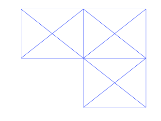
Figure 1: $\mathcal{T}_{0}$ (left) and $\mathcal{T}_{1}$ (right)

$k$	$m_{0}$	$\mathcal{T}_{1}$	$\mathcal{T}_{2}$	$\mathcal{T}_{3}$	$\mathcal{T}_{4}$	$\mathcal{T}_{5}$
0	1	19	18	19	19	19
	2	13	13	14	14	15
	3	10	12	13	13	14
1	1	20	21	21	20	20
	2	13	14	14	15	15
	3	11	12	13	13	14
$\qquad\qquad m_{1}=1$

$k$	$m_{0}$	$\mathcal{T}_{1}$	$\mathcal{T}_{2}$	$\mathcal{T}_{3}$	$\mathcal{T}_{4}$	$\mathcal{T}_{5}$
0	1	17	18	17	17	17
	2	12	12	12	12	12
	3	10	10	10	11	11
1	1	20	20	20	20	19
	2	12	13	13	13	12
	3	10	10	11	11	11
$\qquad\qquad m_{1}=2$

$k$	$m_{0}$	$\mathcal{T}_{1}$	$\mathcal{T}_{2}$	$\mathcal{T}_{3}$	$\mathcal{T}_{4}$	$\mathcal{T}_{5}$
0	1	17	17	17	17	17
	2	12	11	11	11	11
	3	10	9	10	10	10
1	1	20	20	20	19	19
	2	12	13	12	12	12
	3	10	10	10	10	10
$\qquad\qquad m_{1}=3$

Table 1: Numerical results for the first experiment

$k$	$m_{1}$	$\mathcal{T}_{1}$	$\mathcal{T}_{2}$	$\mathcal{T}_{3}$	$\mathcal{T}_{4}$	$\mathcal{T}_{5}$
0	1	22	24	24	23	23
	2	22	23	23	23	22
	3	21	23	23	22	22
1	1	34	34	34	34	34
	2	34	34	34	34	34
	3	34	34	34	34	34

Table 2: Numerical results for the second experiment

In the third experiment, we set $\Omega=(-1,1)\times(-1,1)$ and define $\bm{a}(x,y)=\text{diag}(a(x,y),a(x,y))$ with

$$a(x,y):=\left\{\begin{array}[]{rrr}1,&-1<x<0,&-1<y<0;\\ 7,&0<x<1,&-1<y<0;\\ 17,&0<x<1,&0<y<1;\\ 3,&-1<x<0,&0<y<1.\end{array}\right.$$

We show the first two triangulations $\mathcal{T}_{0}$ and $\mathcal{T}_{1}$ in Figure 2 and produce a sequence of triangulations $\{\mathcal{T}_{j}:j=0,1,\cdots,25\}$ in a successive way: $\mathcal{T}_{j+1}$ ($j=2,3,\cdots,24$) is obtained by refining the smallest square containing the origin in $\mathcal{T}_{j}$ (in $\mathcal{T}_{1}$, the vertexes of the square to refine is in red color) as same as what has been done from $\mathcal{T}_{0}$ to $\mathcal{T}_{1}$. $\mathcal{T}_{25}$ is shown in Figure 3. The difference of the two-level algorithm between this experiment and the first one is that we simply take $\widetilde{\mathcal{R}_{h}}=\widetilde{\mathcal{A}_{h}}^{-1}$ here. The corresponding numerical results are presented in Table 3.

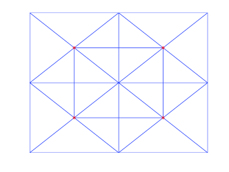
Figure 2: $\mathcal{T}_{0}$ (left) and $\mathcal{T}_{1}$ (right)

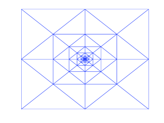
Figure 3: $\mathcal{T}_{25}$

$k$	$m_{0}$	$\mathcal{T}_{5}$	$\mathcal{T}_{10}$	$\mathcal{T}_{15}$	$\mathcal{T}_{20}$	$\mathcal{T}_{25}$
0	1	15	15	15	15	15
	2	12	12	12	12	12
	3	12	12	12	12	12
1	1	30	30	30	30	30
	2	16	16	16	16	16
	3	12	12	12	12	12

Table 3: Numerical results for the third experiment

For the first two examples, the regularity estimate (1.2) holds with only $\alpha\leqslant 0.5$, which violates the regularity requirement $\alpha\in(0.5,1]$ in [19]. For the third example, not only (1.2) holds with $\alpha\leqslant 0.5$, but also the triangulation is not quasi-uniform. However, for all the experiments, the numerical results are consistent with our theoretical results, which shows that our algorithm is convergent even when $\alpha$ is not greater than $0.5$ in (1.2) and the triangulation is not quasi-uniform.

Appendix A Analysis of symmetric Gauss-Seidel iteration

Let $\mathcal{R}_{h}$ be the symmetric Gauss-Seidel iteration. As stated in Remark 3.3, we can show $\mathcal{R}_{h}$ satisfies Assumption III. Suppose Assumption I is true. Then by the well-known properties of Gauss-Seidel iteration, we know that (3.13) holds with $\omega=1$. Thus it remains to verify (3.14).

Let $\{\eta_{i}:i=1,2,\cdots,N\}$ be the standard nodal basis for $M_{h}$. Define $P_{i}:M_{h}\to\text{span}\{\eta_{i}\}$ by

$$\langle P_{i}\lambda_{h},\eta_{i}\rangle_{\mathcal{A}_{h}}=\langle\lambda_{h},\eta_{i}\rangle_{\mathcal{A}_{h}},\quad i=1,2,\cdots,N.$$ (A.1)

By Theorem 3 in [9], we have

$$\langle\mathcal{R}_{h}^{-1}\mu_{h},\mu_{h}\rangle_{h}=\left\lVert\mu_{h}\right\rVert^{2}_{\mathcal{A}_{h}}+\inf_{\sum_{i=1}^{N}\mu_{i}=\mu_{h}}\sum_{i=1}^{N}\left\lVert P_{i}\sum_{j>i}\mu_{j}\right\rVert^{2}_{\mathcal{A}_{h}},~{}\forall\mu_{h}\in M_{h}.$$ (A.2)

Then, by using the same technique used in the proof of Lemma 3.7, we can obtain

$$\langle\mathcal{R}_{h}^{-1}\mu_{h},\mu_{h}\rangle_{h}\lesssim\sum_{T\in\mathcal{T}_{h}}h_{T}^{-2}\left\lVert\mu_{h}\right\rVert^{2}_{h,\partial T}.$$ (A.3)

Denote $\mathcal{S}_{h}:=\mathcal{R}_{h}\mathcal{A}_{h}$. By the definition (3.6) of $\overline{\mathcal{R}_{h}}$, it holds

$$\overline{\mathcal{R}_{h}}=2\mathcal{R}_{h}-\mathcal{R}_{h}\mathcal{A}_{h}\mathcal{R}_{h}=(2\mathcal{S}_{h}-\mathcal{S}_{h}^{2})\mathcal{A}_{h}^{-1},$$ (A.4)

which yields

$$\begin{split}\langle\overline{\mathcal{R}_{h}}^{-1}\lambda_{h},\lambda_{h}\rangle_{h}&=\langle\mathcal{\mathcal{missing}}R_{h}^{-1}S_{h}(2\mathcal{S}_{h}-\mathcal{S}_{h}^{2})^{-1}\lambda_{h},\lambda_{h}\rangle_{h}.\end{split}$$

It is easy to verify that $\mathcal{S}_{h}$ is symmetric with respect to the inner product $\langle\mathcal{R}_{h}^{-1}\cdot,\cdot\rangle_{h}$. Then, from the inequality

$$t(2t-t^{2})^{-1}<1\text{ for all $t\in(0,1)$}$$ (A.5)

and the fact that all the eigenvalues of $\mathcal{S}_{h}$ are in $(0,1)$, it follows

$$\langle\overline{\mathcal{R}_{h}}^{-1}\lambda_{h},\lambda_{h}\rangle_{h}\leqslant\langle\mathcal{R}_{h}^{-1}\lambda_{h},\lambda_{h}\rangle_{h},$$ (A.6)

which, together with (A.3), leads to the desired result (3.14).

References

- [1] B. AKSOYLU, M. HOLST, Optimality of multilevel preconditioners for local mesh refinement in three dimensions, SIAM J. Numer. Anal., 44 (2006), 1005-1025.
- [2] D. N. ARNOLD, F. BREZZI, Mixed and non-conforming finite element methods: implementation, post-processing and error estimates, Modél. Math. Anal. Numér., 19 (1985), 7-35.
- [3] F. BORNEMANN, B. ERDMANN, R. KORNHUBER, Adaptive multilevel methods in three space dimensions, Int. J. for Numer. Meth. in Eng., 36 (1993), 3187-3203.
- [4] A. BRANDT, Multi-level adaptive solutions to boundary-value problems, Math. Comp., 31 (1977), 333-390.
- [5] A. BRANDT, S. F. MCCORMICK, J. W. RUGE, Algebraic Multigrid (AMG) for Automatic Multigrid Solution with Application to Geodetic Computations, Technical report, Institute for Computational Studies, Colorado State University, Fort Collins, CO, 1982.
- [6] A. BRANDT, Algebraic multigrid theory: The symmetric case, Appl. Math. Comput., 19 (1986), 23-56.
- [7] F. BREZZI, J. DOUGLAS, JR., L. D. MARINI, Two families of mixed finite elements for second order elliptic problems, Numer. Math., 47 (1985), 217-235.
- [8] Z. CHEN, Equivalence between and multigrid algorithms for mixed and nonconforming methods for second order elliptic problems, East-West J. Numer. Math., 4 (1994), 1-33.
- [9] L. CHEN, Deriving the X-Z identity from auxiliary space method, In: The Proceedings for 19th Conferences for Domain Decomposition Methods, 2010.
- [10] L. CHEN, R. H. NOCHETTO, J. XU, Optimal multilevel methods for graded bisection grids, Numer. Math., 120 (2011), 1-34.
- [11] L. CHEN, J. WANG, Y. WANG, X. YE, An auxiliary space multigrid preconditioner for the weak Galerkin method, arXiv preprint arXiv:1410.1012, 2014.
- [12] D. CHO, J. XU, L. ZIKATANOV, New estimates for the rate of convergence of the method of subspace corrections, Numer. Math. Theor. Meth. Appl., 1 (2008), 44-56.
- [13] B. COCKBURN, J. GOPALAKRISHNAN, A characterization of hybridized mixed methods for second order elliptic problems, SIAM J. Numer. Anal., 42 (2004), 283-301.
- [14] B. COCKBURN, J. GOPALAKRISHNAN, New hybridization techniques, GAMM-Mitt, 2 (2005), 154-183.
- [15] B. COCKBURN, J. GOPALAKRISHNAN, AND H. WANG, Locally conservative fluxes for the continuous Galerkin method, SIAM J. Numer. Anal., 45 (2007), 1742-1776.
- [16] B. COCKBURN, B. DONG, J. GUZMÁN, A superconvergent LDG-hybridizable Galerkin method for second-order elliptic problems, Math. Comp., 77 (2008), 1887-1916.
- [17] B. COCKBURN, J. GOPALAKRISHNAN, R. LAZAROV, Unified hybridization of discontinuous Galerkin, mixed, and conforming Galerkin methods for second order elliptic problems, SIAM J. Numer. Anal., 47 (2009), 1319-1365.
- [18] B. COCKBURN, J. GOPALAKRISHNAN, F. J. SAYAS, A projection-based error analysis of HDG methods, Math. Comp., 79 (2010), 1351-1367.
- [19] B. COCKBURN, O. DUBOIS, J. GOPALAKRISHNAN, S. TAN, Multigrid for an HDG method, IMA Journal of Numerical Analysis, 34 (2014), 1386-1425.
- [20] W. DAHMEN, A. KUNOTH, Multilevel preconditioning, Numer. Math., 63 (1992), 315-344.
- [21] J. GOPALAKRISHNAN, A Schwarz preconditioner for a hybridized mixed method, Comput. Methods Appl. Math., 3 (2003), 116-134.
- [22] J. GOPALAKRISHNAN, S. TAN, A convergent multigrid cycle for the hybridized mixed method, Numer. Linear Algebra Appl., (2009), 689-714.
- [23] B. LI, X. XIE, A two-level algorithm for the weak Galerkin discretization of diffusion problems, arXiv preprint arXiv:1405.7506v3, 2014.
- [24] B. LI, X. XIE, Analysis of a family of HDG methods for second order elliptic problems, arXiv preprint arXiv:1408.5545, 2014.
- [25] B. LI, X. XIE, BPX preconditioner for nonstandard finite element methods for diffusion problems, arXiv preprint parXiv:1410.5332v1.
- [26] O. E. LIVNE, Coarsening by compatible relaxation, Numer. Linear Algebra Appl., 11 (2004), 205-227.
- [27] S. MCCORMICK, Fast adaptive composite gird (FAC) methods: theory for the variational case, In Defect correction methods (Oberwolfach, 1983), volume 5 of Comput. Suppl., Springer, Vienna, 1984, 115-121.
- [28] S. F. MCCORMICK, J. W. THOMAS, The fast adaptive composite grid (FAC) method for elliptic equations, Math. Comp., 46 (1986), 439-456.
- [29] L. MU, J. WANG, Y. WANG, X. YE, A computational study of the weak Galerkin method for second-order elliptic equations, arXiv:1111.0618v1, 2011, Numerical Algorithms, 2012, DOI:10.1007/s11075-012-9651-1.
- [30] L. MU, J. WANG, X. YE, A weak Galerkin finite element methods with polynomial reduction, arXiv:1304.6481, submited to SIAM J on Scientific Computing.
- [31] L. MU, J. WANG, X. YE, Weak Galerkin finite element methods on polytopal meshes, arXiv:1204.3655v2, submitted to International J of Nmerical Analysis and Modeling.
- [32] P.-A. RAVIART, J. M. THOMAS, A mixed finite element method for second order elliptic problems, Mathematical Aspects of Finite Element Method (I. Galligani and E. Magenes, eds.), Lecture Notes in Math. 606, Springer-Verlag, New York, 1977, 292-315.
- [33] P. VANĚK, J. MANDEL, M. BREZINA, Algebraic multigrid by smoothed aggregation for second and fourth order elliptic problems, Computing, 56 (1996), 179-196.
- [34] J. WANG, X. YE, A weak Galerkin finite element method for second-order elliptic problems, J. Comp. Appl. Math., 241 (2013), 103-115.
- [35] H. WU, Z. CHEN, Uniform convergence of multigrid V-cycle on adaptively refined finite element meshes for second order elliptic problems, Science in China: Series A Mathematics, 49 (2006), 1-28.
- [36] J. XU, L. ZIKATANOV, The method of alternating projections and the method of subspace corrections in Hilbert space, J. Am. Math. Soc., 15 (2002), 573-597.