Revisiting linear augmentation for stabilizing stationary solutions: potential pitfalls and their application

Abstract

Linear augmentation has recently been shown to be effective in targeting desired stationary solutions, suppressing bistablity, in regulating the dynamics of drive response systems and in controlling the dynamics of hidden attractors. The simplicity of the procedure is the highlight of this scheme but at the same time questions related to its general applicability still need to be addressed. Focusing on the issue of targeting stationary solutions, this work demonstrates instances where the scheme fails to stabilize the required solutions and leads to other complicated dynamical scenarios. Appropriate examples from conservative as well as dissipative systems are presented in this regard and potential applications for relevant observations in dissipative predator–prey systems are also discussed.

I Introduction

Studies on coupled nonlinear systems have explored a wide variety of emergent dynamical phenomena, namely synchronization Pikovsky et al. (2001), oscillator suppression Saxena et al. (2012); Koseska et al. (2013), multistability Feudel (2008), hysteresis Prasad et al. (2005), extreme–events Ansmann et al. (2013); Karnatak et al. (2014a) etc. which can be exploited in applications, to model natural phenomena or in regulating the system behavior for instance. Controlling dynamical systems towards a desired behavior is an important research topic in nonlinear sciences Schöll and Schuster (2008). Starting with chaos control Ott et al. (1990); Pecora and Carroll (1990); Pyragas (1992); Peng et al. (1996), research in this domain now also extends towards control of multistability Pisarchik and Feudel (2014), patterns and spatio–temporal chaos Gang and Zhilin (1994); Boccaletti et al. (1999), noisy systems Balanov et al. (2004); Hauschildt et al. (2006), methods of stabilizing unstable stationary solutions Bar-Eli (1984); Saxena et al. (2012); Koseska et al. (2013) etc. A greater understanding of these different regulatory aspects have greatly contributed towards development of related novel and highly efficient procedures. Considering noninvasive (without changing the intrinsic system parameters) mechanisms leading to stabilization of stationary solutions, oscillator suppression via coupling nonlinear systems has been discussed extensively in literature (see Refs. Saxena et al. (2012); Koseska et al. (2013) for detailed reviews). This suppression is majorly observed as a consequence of parameter heterogeneity between the coupled units Ermentrout (1990); Aronson et al. (1990); Mirollo and Strogatz (1990), presence of time–delayed Ramana Reddy et al. (1998); Atay (2003)/conjugate variables Karnatak et al. (2007) in the coupling function or through dynamic coupling Konishi (2003).

Recently, linear augmentation has also been suggested as another practical alternative leading to oscillator suppression, achieved by coupling systems to a linear feedback consisting of a simple decaying function Sharma et al. (2011). Lately, studies have also used linear augmentation effectively for controlling bistability Sharma et al. (2013), dynamics of a drive response system Sharma et al. (2014) and in controlling the dynamics of hidden attractors Sharma et al. (2015). With respect to stabilizing stationary solutions, Ref. Sharma et al. (2011) discussed results for an augmented Lorenz system where either the stationary solutions of the original system or those of the augmented system could be stabilized by picking an appropriate feedback function; former being quite relevant from an application perspective. The paper also presented some parameter space scans highlighting the regimes where linear augmentation works and where it does not, which although is instructive but is also very system specific at the same time. At this point, one must question the ability of linear augmentation towards stabilizing the stationary solutions in a more general sense, namely the systems, parameter settings and coupling configurations where the scheme works and where it does not? In this paper, we will look at some simple examples of linearly augmented systems demonstrating the fact that we need to be quite careful before picking linear augmentation in applications. These examples illustrate that there could be situations where even picking an appropriate feedback function does not guarantee that the required stationary solutions will be necessarily stabilized. We will see that the mechanism appears to be highly dependent on the intrinsic properties of the oscillators in consideration, the stationary solutions we want to target, and also on how these systems are augmented by/coupled to the feedback. Furthermore, we will also discuss instances where the failures of the procedure can be exploited in applications.

The manuscript is arranged as follows: Linear augmentation is introduced in the following Sec. II. In Sec. III, we will have a look at results for linearly augmented conservative and dissipative dynamical systems. In Sec. III.1, results for partially and fully augmented harmonic oscillator are presented, Sec. III.2 discusses results for conservative Duffing oscillator under similar augmentations, and in Sec III.3, we will have a look at the behavior of augmented dissipative population models and also briefly discuss possible applications for certain observations in these systems. The manuscript concludes with a summary of results in Sec. IV. Additional details on certain dynamical aspects of harmonic oscillator and Duffing system which were excluded from main manuscript are provided in Appendices A, B, and C.

II Linear augmentation

General representation of a linearly augmented dynamical system is,

$$\left.\begin{array}[]{l}\dot{{\bf x}}={\bf f(x)}+\bm{\varepsilon}u\\ \dot{u}=-ku-\bm{\varepsilon}(\mathbf{x-b})^{T}.\\ \end{array}\right\}$$ (1)

where the column vector $\mathbf{x}=[x_{1},x_{2},\ldots,x_{N}]^{T}\in\mathbb{R}^{N}$ ($[...]^{T}$ corresponds to the transpose) contains the systems variables, and $u$ is the augmentation variable. $\bm{\varepsilon}=[\varepsilon_{1},\varepsilon_{2},\ldots,\varepsilon_{N}]^{T}\in\mathbb{R}^{N}$ is a column vector with information regarding the coupling strength of the interaction between the dynamical variables and $u$; augmentation/coupling term corresponding to the $i^{th}$ component $x_{i}$ is $\varepsilon_{i}u$ $\forall$ $i=1,2,\ldots,N$, and $\varepsilon_{i}=0$ if $x_{i}$ is not coupled to $u$. $\mathbf{b}\in\mathbb{R}^{N}$ is an arbitrary vector and $k$ is the decay constant Resmi et al. (2010) which could be used to control the transient time leading to stabilization of stationary solutions Sharma et al. (2011). Vector $\mathbf{b}=\mathbf{x^{*}}=[{x_{1}}^{*},{x_{2}}^{*},\ldots,{x_{N}}^{*}]^{T}\in\mathbb{R}^{N}$ where $\mathbf{x^{*}}$ satisfies $\dot{{\bf x}}|_{\mathbf{x=x^{*}}}={\bf f(x^{*})}=\mathbf{0}$ if we want to stabilize a stationary solution $\mathbf{x^{*}}$ of the original system. Substituting a value of $\mathbf{b}\neq\mathbf{x^{*}}$ can stabilize stationary solutions of augmented system for which $\mathbf{\dot{X}}=[\dot{x_{1}},\dot{x_{2}},\ldots,\dot{x_{N}},\dot{u}]^{T}\in\mathbb{R}^{N+1}=\mathbf{0}$. The term $\bm{\varepsilon}(\mathbf{x-b})^{T}$ gives the dot product of the corresponding column vectors.

In the following, we will look at examples of augmented conservative as well as dissipative dynamical systems which highlight the limitations of this procedure. The terms augmentation/augmented and coupling/coupled have been used synonymously in the following text.

III Examples

Here we will discuss the instances of systems controlled via linear augmentation. We will first look at two examples of conservative systems, namely the harmonic oscillator and conservative Duffing oscillator where linear augmentation will be used to stabilize their stationary solutions.

III.1 Harmonic oscillator

Figure 1: (Color online) a) Bifurcation diagram (black dots), largest eigenvalues (red symbols) and the time series of $x$ variable before and after the stabilization of origin as inset. Corresponding phase space plots are in b) (no augmentation: $\varepsilon=0$) and c) (with augmentation: $\varepsilon=0.5$). d) Variation in the eigenvalues for higher values of augmentation strength $\varepsilon$. Parameter values for calculation are $\omega=2$ and $k=2$.

Equations describing a linearly augmented harmonic oscillator are:

$$\dot{x} = y+\varepsilon u,$$

$$\dot{y} = -{\omega}^{2}x,$$

$$\dot{u} = -ku-\varepsilon x,$$ (2)

where $\omega$ is the frequency of the oscillator, $k$ is the augmentation parameter, and $\varepsilon$ is the coupling strength. The first two equations governing the evolution of $x$ and $y$ correspond to the original harmonic oscillator dynamics. In the absence of augmentation, harmonic oscillator conserves total energy, which stays constant on the ellipses shown in Fig. 1 b). Each of these ellipses correspond to the system evolution following different initial values of position and momentum, and hence, different conserved total energies. Harmonic oscillator has $x^{*}=0,y^{*}=0$ as the only stationary solution and note that the augmentation term only appears in the rate equation of the position variable $x$ at this point. In case of a successful stabilization, the required stationary solution of the full system should be $(x^{*},y^{*},u^{*})=(0,0,0)$ (origin) where the system effectively decouples from augmentation.

The characteristic eigenvalue equation at the origin is,

$$(\lambda+k)(\lambda^{2}+\omega^{2})+\varepsilon^{2}\lambda=0.$$ (3)

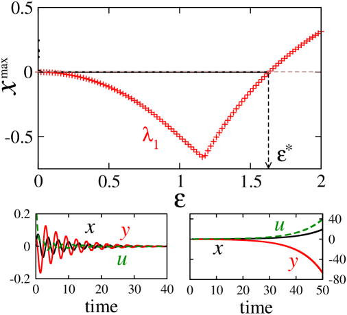
For $\varepsilon=0$, the eigenvalues for the full system are $\lambda_{1,2}=\pm i\omega$ which correspond to the non-hyperbolic stationary solution at the origin, and $\lambda_{3}=-k$ corresponding to the decay of the augmentation variable $u$; which evolves as $u(t)\propto exp(-kt)$ in this case. The parameter values for the following calculations were fixed at $\omega=2$, and $k=2$. For the evolution of the augmented system ($\varepsilon>0$), the bifurcation diagram bif of the system with increasing $\varepsilon$ values is shown in Fig. 1 a) (black dots). It is seen that with an increasing $\varepsilon$, the system which was conservative for $\varepsilon=0$ becomes dissipative and gets into a stable origin regime even for quite small values of $\varepsilon$. Rewriting Eq. 3 as,

$$\lambda^{3}+k\lambda^{2}+(\omega^{2}+\varepsilon^{2})\lambda+k\omega^{2}=0,$$ (4)

and applying the Routh–Hurwitz criteria (RHC) Rou , we can deduce that the roots of this equation are all either negative or have negative real parts (in case of complex roots) $\forall$ $\varepsilon>0$. Largest eigenvalues of the Jacobian (red symbols) are also plotted along with the bifurcation diagram in Fig. 1 a) which demonstrate the transition from oscillatory to stationary state for $\varepsilon>0$. Considering the behavior of this system for large $\varepsilon$, we can see that the largest eigenvalue $\lambda=\lambda_{1}\to 0$ from Eq. 4 in this limit. Since the discriminant dis of the cubic characteristic Eq. 4 is negative $\forall$ $\varepsilon\geq 0$, this implies that the system has one real eigenvalue and a pair of complex conjugate eigenvalues in this range. The negative real part of these complex eigenvalues for large $\varepsilon$ can therefore be estimated by equating the sum of all eigenvalues to the trace of the Jacobian $\text{tr}(J)$, giving $\text{Re}(\lambda_{2,3})=-k/2$. This further implies that as $\varepsilon\to\infty$, convergence to the origin gets slower although origin is stable in the entire $\varepsilon>0$ range and any change in stability will only occur as $\varepsilon\to\infty$ when $\lambda_{1}=0$.

Now let us consider a more general case of an augmented harmonic oscillator given by,

$$\dot{x} = y+\varepsilon_{1}u,$$

$$\dot{y} = -{\omega}^{2}x+\varepsilon_{2}u,$$ (5)

$$\dot{u} = -ku-\varepsilon_{1}x-\varepsilon_{2}y,$$

where the augmentation now appears in the rate equations of both position $x$ and momentum $y$ with coupling strengths $\varepsilon_{1}$, $\varepsilon_{2}$ respectively. The eigenvalue equation in this case is,

$$(\lambda+k)(\lambda^{2}+\omega^{2})+\lambda({\varepsilon_{1}}^{2}+{\varepsilon_{2}}^{2})+\varepsilon_{1}\varepsilon_{2}(1-\omega^{2})=0.$$

(6)

Substituting $\varepsilon_{2}=0$ and $\varepsilon_{1}=\varepsilon$ in Eq. 6 yields the dynamics of Eq. 2. Similarly, for $\varepsilon_{1}=0$ and $\varepsilon_{2}=\varepsilon$, we obtain a case where the system is only coupled in the $y$ variable for which the characteristic Eq. 6 is exactly identical to Eq. 4, and therefore the stability characteristics of the origin are identical and independent of whether the system is augmented in $x$ or $y$. In the previous example, we saw a situation where linear augmentation successfully stabilized the origin for the entire range of $\varepsilon>0$. Now considering $\varepsilon_{1}=\varepsilon_{2}=\varepsilon$ (the system is similarly augmented in both variables), in which case Eq. 6 gives,

$$\lambda^{3}+k\lambda^{2}+(\omega^{2}+2\varepsilon^{2})\lambda+k\omega^{2}+\varepsilon^{2}(1-\omega^{2})=0.$$ (7)

Using the RHC, it can be seen that this equation will have all negative eigenvalues iff $k\omega^{2}+\varepsilon^{2}(1-\omega^{2})>0$ which gives a stability regime of $0<\varepsilon<\varepsilon^{*}$ $\forall$ $\omega>1$ where $\varepsilon^{*}=\omega\sqrt{\dfrac{k}{\omega^{2}-1}}$, and for higher values of $\varepsilon$, RHC suggests appearance of positive eigenvalue/eigenvalues. For large $\varepsilon$, we can get an estimate of largest eigenvalue $\lambda_{1}\to\dfrac{(\omega^{2}-1)}{2}>0$ $\forall$ $\omega>1$. Since the discriminant is negative $\forall$ $\varepsilon>0$, the remaining complex conjugate eigenvalue pair have a negative real part given by $\text{Re}(\lambda_{2,3})=(\text{Tr}(J)-\lambda_{1})/2=-\left(\dfrac{k}{2}+\dfrac{(\omega^{2}-1)}{4}\right)$. Therefore, unlike in the previous example, we can see that origin here is unstable for large $\varepsilon$. The expression for $\varepsilon^{*}$ also shows that a higher value of $k$ can extend the coupling range for a stable origin. This result is the first instance of unexpected behavior as we would normally expect a higher coupling value to keep the origin stable. Furthermore, in the $\varepsilon>\varepsilon^{*}$ regime it is numerically observed that the trajectories escape to infinity which is also quite unexpected.

One of the primary reasons behind considering augmented harmonic oscillator in this study is the fact that it is highly solvable and therefore can provide necessary insights into the physical mechanisms behind the desirable as well as undesirable behaviors. It turns out that in case of a successful stabilization, this system represents a forced harmonic oscillator where the steady state solution (which is completely determined by the forcing) decays to the origin along with an exponentially decaying force. Similarly, the case where the trajectories escape to infinity corresponds again to a forced system but this time being driven by an exponentially diverging force which is analogous to a situation where energy is being pumped into the system. Therefore the steady state solution in this case diverges along with the diverging force explaining the unexpected behavior of escaping trajectories observed for the fully augmented system. Details of the calculations leading to these deductions are available in Appendix A.

III.2 Duffing oscillator

Figure 2: (Color online) Largest eigenvalue estimates for stationary solutions $(x^{*},y^{*})=(0,0)$ (black), $(x^{*},y^{*})=(\pm 1,0)$ (red) for partially augmented Duffing system.

General equations for a linearly augmented Duffing oscillator with no damping or forcing can be written as:

$$\dot{x} = y+\varepsilon_{1}u,$$

$$\dot{y} = x-x^{3}+\varepsilon_{2}u,$$

$$\dot{u} = -ku-\varepsilon_{1}(x-x^{*})-\varepsilon_{2}(y-y^{*}).$$ (8)

Uncoupled Duffing system has an invariant of motion (also the Hamiltonian of the system) given by $H(x,y)=y^{2}/2-x^{2}/2+x^{4}/4$ and stationary solutions: $(x^{*},y^{*})=(\pm 1,0),(0,0)$. The trajectories of this system evolve on the double well potential surface of $H(x,y)$ starting from different initial conditions for $\varepsilon_{1}=\varepsilon_{2}=0$. Similar to the previous example, for a successful stabilization, the required stationary solutions of the full system should be $(x^{*},y^{*},u^{*})=(0,0,0)$ or $(\pm 1,0,0)$ where the system effectively decouples from the augmentation. These solutions will be referred to as $(x^{*},y^{*})=(0,0)$ (origin) or $(\pm 1,0)$ in the following.

For the system in Eq. 8, the characteristic eigenvalue equation can be expressed as,

$$(\lambda+k)(\lambda^{2}+3{x^{*}}^{2}-1)+\lambda({\varepsilon_{1}}^{2}+{\varepsilon_{2}}^{2})$$

$$+\varepsilon_{1}\varepsilon_{2}(2-3{x^{*}}^{2})=0.$$ (9)

Now similar to the harmonic oscillator example, considering partial augmentation with $\varepsilon_{1(2)}=\varepsilon$, and $\varepsilon_{2(1)}=0$ first, Eq. 9 suggests that the stability characteristics for the stationary solutions are again independent of whether the system is being augmented in $x$ or $y$. For this partial augmentation, Eq. 9 gives,

$$(\lambda+k)(\lambda^{2}+3{x^{*}}^{2}-1)+\lambda{\varepsilon}^{2}=0.$$ (10)

Substituting $x^{*}=0,\pm 1$, and rearranging the terms, we can obtain the characteristic eigenvalue equations for these stationary solutions as,

$$\lambda^{3}+k\lambda^{2}+(\varepsilon^{2}-1)\lambda-k=0,$$ (11)

for $(x^{*},y^{*})=(0,0)$ (hyperbolic for $\varepsilon=0$), and

$$\lambda^{3}+k\lambda^{2}+(\varepsilon^{2}+2)\lambda+2k=0,$$ (12)

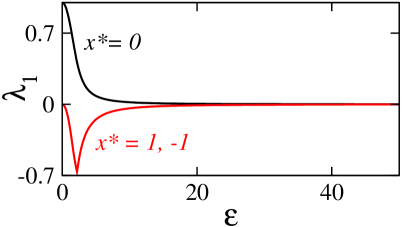
for $(x^{*},y^{*})=(\pm 1,0)$ (non hyperbolic for $\varepsilon=0$) respectively. It is straightforward to check that the largest eigenvalue $\lambda_{1}\to 0$ for larger $\varepsilon$ values in both these cases which implies that a stable/unstable stationary solution will retain its stability characteristics until a stability change (zero crossing of the eigenvalue/s) occurs in the $\varepsilon\to\infty$ limit. Furthermore using the RHC, it is easily verifiable that Eq. 11 will always have positive root/roots, whereas Eq. 12 will have all negative roots $\forall$ $\varepsilon>0$; which implies that the $x^{*}=0$ is always unstable and $x^{*}=\pm 1$ is always stable. Therefore, we see that partial augmentation works for stabilizing $(x^{*},y^{*})=(\pm 1,0)$ but fails completely to stabilize the origin $(x^{*},y^{*})=(0,0)$. Fig. 2 shows the largest eigenvalue calculations which verify these deductions. This brings us to an important observation that there might exist situations where it is not possible to target the required stationary solution even on using an appropriate feedback function with any combination of $k$ and $\varepsilon$ values.

Figure 3: (Color online) Figs. a), b) and c) show the bifurcation diagrams (black dots) and the largest eigenvalues (red symbols) for $(x^{*},y^{*})=(1,0),(0,0)$, and $(-1,0)$ respectively. Related Figs. a.1: for $\varepsilon=0.4$, the system is bistable and the two related transient behaviors (in blue and green and likewise for other cases), a.2: for $\varepsilon=1$, the trajectory approaching the stable stationary solution $(1,0)$, and a.3 shows an arbitrary time series for $\varepsilon=2.5$. Similarly in b.1: bistability, and in b.2: the system approaching the stable stationary solution $(0,0)$ is shown. Identically, c.1, c.2, and c.3 show the bistability ($\varepsilon=0.4$), stabilization of $(-1,0)$ ($\varepsilon=1)$ and an arbitrary time series at $\varepsilon=2.5$.

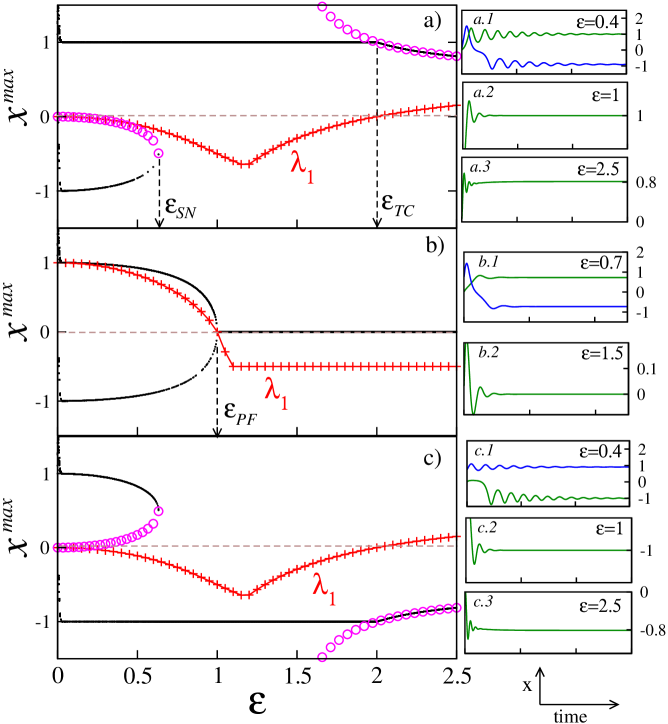
Now considering identical augmentation with $\varepsilon_{1}=\varepsilon_{2}=\varepsilon$ and we will see that this system has some interesting properties. Fig. 3 shows the bifurcation diagrams bif of the system as we try targeting different stationary solutions: For $(x^{*},y^{*})=(1,0)$, the bifurcation diagram (black dots) is shown in Fig. 3 a). Appropriate transient trajectories in different coupling regimes are also shown in related Figs. 3 (a.1), (a.2), (a.3). It is observed that even for very small coupling values, the system quickly gets into a stable stationary state regime, although, for smaller values of $\varepsilon$, it exhibits bistability. The transient trajectories in this parameter regime are shown in Fig. 3 (a.1). We observe that the augmentation is stabilizing our desired stationary solution at $(x^{*},y^{*})=(1,0)$, but along with it, other stationary solutions which are $\varepsilon$ dependent are also getting stabilized on starting with different initial conditions. These other stationary solutions for the augmented system here are given by,

$${x^{*}}_{\pm} = \dfrac{1}{2}\left(-1\pm\sqrt{1-\dfrac{4\varepsilon^{2}}{k-\varepsilon^{2}}}\right),$$

$${y^{*}}_{\pm} = {x^{*}}_{\pm}-{{x^{*}}_{\pm}}^{3},$$

$${u^{*}}_{\pm} = -\dfrac{{y^{*}}_{\pm}}{\varepsilon},$$ (13)

and solutions $({x^{*}}_{-},{y^{*}}_{-},{z^{*}}_{-})$ are observed to coexist along with $(x^{*},y^{*})=(1,0)$. For higher coupling values, bistability terminates via a saddle node bifurcation when the stable branch of stationary solutions $({x^{*}}_{-},{y^{*}}_{-},{u^{*}}_{-})$ collides with the unstable branch of $({x^{*}}_{+},{y^{*}}_{+},{u^{*}}_{+})$(circles) as shown in in Fig. 3 (a) at $\varepsilon_{SN}=\sqrt{\dfrac{k}{5}}$. The system also exhibits hysteresis in this bistable regime and a brief discussion regarding this observation is available in Appendix B. Beyond this regime for a range of values in $\varepsilon>\varepsilon_{SN}$, $(x^{*},y^{*})=(1,0)$ remains as the only stable attractor as shown in Fig. 3 (a),(a.2).

In absence of augmentation, the eigenvalues for $(x^{*},y^{*})=(1,0)$ are complex: $\lambda_{1,2}=\pm i\sqrt{2}$. For the augmented system, the characteristic equation can therefore be written as:

$$\lambda^{3}+k\lambda^{2}+2\lambda(1+\varepsilon^{2})+(2k-\varepsilon^{2})=0.$$ (14)

The RHC shows that this equation will have all negative roots for $(2k-\varepsilon^{2})>0$ and positive root/roots appear for $\varepsilon>\sqrt{2k}$. This gives us the transition threshold for the destabilization of the stationary solution as $\varepsilon^{*}=\sqrt{2k}$, at which the eigenvalue/s cross the zero axis. Since the discriminant is negative, the characteristic equation has one real and two complex conjugate roots. Considering large $\varepsilon$ behavior, it is seen that the largest eigenvalue $\lambda_{1}\to 1/2$ which implies that $(x^{*},y^{*})=(1,0)$ is unstable in this range. The real part of the remaining complex conjugate eigenvalue pair is $\text{Re(}\lambda_{2,3}\text{)}=-(2k+1)/4$. At $\varepsilon^{*}$, Eq. 14 can be rewritten as,

$$\lambda(\lambda^{2}+k\lambda+2(1+2k))=0,$$ (15)

which consequently gives the eigenvalues as $\lambda_{1}=0$ and $\lambda_{2,3}=(-k\pm\sqrt{k^{2}-8(1+2k)})/2$. We can see that $\lambda_{2,3}$ will be a complex conjugate pair for $k\in(8-6\sqrt{2},8+6\sqrt{2})$. For our calculations, we have taken $k=2$ which shows that at $\varepsilon^{*}=\sqrt{2k}=2$, $\lambda_{1}$ crosses the zero line as can be seen in Fig. 3 a) (red symbols). For higher values of $\varepsilon>\sqrt{2k}$, stationary states $({x^{*}}_{+},{y^{*}}_{+},{u^{*}}_{+})$ (circles) in Fig. 3 (a) for $\varepsilon>\varepsilon^{*}(=\varepsilon_{TC})$ get stabilized via a transcritical bifurcation where $(x^{*},y^{*})=(1,0)$ and $({x^{*}}_{+},{y^{*}}_{+},{u^{*}}_{+})$ exchange their stability. This again is quite unexpected since the feedback is designed to stabilize $(x^{*},y^{*})=(1,0)$ for higher $\varepsilon$ values. A brief discussion regarding the behavior of this system in the $(\varepsilon,k)$ plane is available in Appendix C.

For the origin at $(x^{*},y^{*})=(0,0)$, the bifurcation diagram (black dots) is shown in Fig. 3 b). Appropriate transient trajectories corresponding to different augmentation regimes are also shown in related Figs. 3 (b.1), (b.2). We observe bistability for a range of lower $\varepsilon$ values before the origin gets stabilized. The stationary solutions obtained in the bistable regime are given by

$${x^{o}}_{\pm} = \pm\sqrt{1-\dfrac{\varepsilon^{2}}{k-\varepsilon^{2}}},$$

$${y^{o}}_{\pm} = {x^{o}}_{\pm}-{{x^{o}}_{\pm}}^{3},$$

$${u^{o}}_{\pm} = -\dfrac{{y^{o}}_{\pm}}{\varepsilon}.$$ (16)

Transient trajectories in this regime demonstrating the two observed stationary solutions are shown in Fig. 3 (b.1). These solutions approach and collapse at the origin at a pitchfork bifurcation for $\varepsilon_{PF}=\sqrt{\dfrac{k}{2}}$ (=1 for $k=2$ in this case) beyond which the solutions $({x^{o}}_{\pm},{y^{o}}_{\pm},{u^{o}}_{\pm})$ become imaginary and the origin is the only stable real stationary solution. A transient trajectory in this parameter regime is shown in Fig. 3 (b.2).

The characteristic equation for the origin is,

$$\lambda^{3}+k\lambda^{2}+\lambda(2\varepsilon^{2}-1)+2\varepsilon^{2}-k=0,$$ (17)

which has all negative eigenvalues for $2\varepsilon^{2}-k>0$ giving us a stability regime of $\varepsilon>\sqrt{k/2}$ and a transition value of $\varepsilon_{PF}=\varepsilon^{*}=\sqrt{k/2}=1$ (since $k=2$) when the eigenvalue/s cross the zero axis. From Eq. 17, we get $\lambda_{1}=-1$ in the large $\varepsilon$ limit. It is numerically observed here that the discriminant $\Delta<0$ in this range and therefore $\text{Re(}\lambda_{2,3}\text{)}=(1-k)/2=-0.5$ and consequently, the origin is stable in the large $\varepsilon$ limit. The largest eigenvalue for the origin is plotted as red symbols in Fig. 3 (b) which shows the changes in the stability of the origin from unstable in $\varepsilon\in(0,1)$ to stable $\forall$ $\varepsilon>1$. For a discussion regarding the system behavior in the $(\varepsilon,k)$ plane, please see Appendix C.

For $(x^{*},y^{*})=(-1,0)$, the bifurcation diagram (black dots) is shown in Fig. 3 c). Appropriate transient trajectories corresponding to different augmentation regimes are also shown in related Figs. 3 (c.1), (c.2), (c.3). Since this solution is a symmetric counterpart of $(x^{*},y^{*})=(1,0)$, the corresponding analysis similarly carries over in this case.

These simple examples demonstrate the fact that targeting the required stationary solutions using linear augmentation is not quite straightforward and the procedure is quite sensitive to how the systems are augmented, the stationary solutions being targeted and to the properties of systems. In the following, results for a specific class of dissipative dynamical systems are presented to further highlight these limitations.

III.3 Dissipative predator–prey models

Figure 4: (Color online) Bifurcation diagram (black dots), largest eigenvalues (red circles) and time series (insets for specific $\varepsilon$ values) for predator–prey systems with H II (left column) and H III (right column) functional responses. Top row: For augmented prey, insets show the time series of $x,y$ and $u$ for two different $\varepsilon$ values before (with oscillatory $u$) and after the stabilization of $(x^{*},y^{*})=(0,0)$ (with $u^{*}=0$). The Hopf bifurcation is marked as $H$, and the transcritical bifurcation points have been highlighted by $T_{1}$, and $T_{2}$ respectively. Middle row: For augmented predator, the systems exhibit oscillatory behavior similar to augmented preys (not shown) for low $\varepsilon$ before they settle on the stationary solution $(x^{*},y^{*})=(K,0)$ with $u^{*}=0$; where the preys reach their carrying capacity in the absence of predators for higher $\varepsilon$ values. Bottom row: For augmented predator and prey, for low $\varepsilon$, the systems are oscillatory (not shown). With increasing $\varepsilon$, both the systems lose the oscillatory behavior and all trajectories escape to infinity (gap in the bifurcation diagram with no black dots). For higher $\varepsilon$ values, unrealistic stationary solutions where either the preys exceed their carrying capacity $(x^{*}>K)$ with negative predator populations $(y^{*}<0)$ (H II and H III), or where the prey populations are negative with small positive predator population (for H II) and $u^{*}\neq 0$ get stabilized.

Considering predator–prey population models, general evolution equations for these systems with logistic prey growth can be written as,

$$\dot{x} = rx(1-x/K)-f(x)y,$$

$$\dot{y} = (\rho f(x)-\gamma)y,$$ (18)

where $x$ and $y$ correspond to prey and predator populations respectively and the parameters $r,K,\rho$, and $\gamma$ are positive. Considering the evolution equation for preys, the first term $rx(1-x/K)$ represents the logistic growth rate of the prey species with the maximum growth rate of $r$ and carrying capacity $K$ which is the maximum population size that the environment can sustain indefinitely. The second term $f(x)y$ corresponds to the prey mortality via predation. $f(x)$ is the functional response governing the rate of per capita prey consumption by the predators Solomon (1949); Holling (1959a, b). The parameter $\rho$ governs the biomass conversion efficiency for the predators in the sense of how many predators are added to the population via predation, and $\gamma$ is the intrinsic predator mortality parameter. One of the stationary solutions of this system corresponds to vanishing predator-prey populations, i.e. $(x^{*},y^{*})=(0,0)$. The other stationary solutions are dependent on the type of functional response considered. Most commonly employed $f(x)$ forms in such models are the Holling type with the following general expressions:

1. $f(x)=ax$ for Holling type I response which is identical to the predation in the Lotka–Volterra case Lotka (1910); Volterra (1926),

2. $f(x)=\dfrac{ax}{(b+x)}$ for Holling type II (Michaelis–Menten kinetics), using which, Eq. 18 gives the Rosenzweig–MacArthur model Rosenzweig and MacArthur (1963),

3. $f(x)=\dfrac{ax^{2}}{(b^{2}+x^{2})}$ for Holling type III (Hill equation type), using which, Eq. 18 gives the Truscott–Brindley model Truscott and Brindley (1994) which is used in modeling phytoplankton and zooplankton interactions leading to harmful algal blooms,

and consequently, corresponding stationary solutions can be obtained. The parameter $a$ in expressions above corresponds to the maximum per capita predation rate, and $b$ is the half saturation constant governing how quickly the predators attain their maximum consumption rate. In the following, we will have a closer look at the stability properties of the trivial stationary solution $(x^{*},y^{*})=(0,0)$: origin. Considering a general augmented population model,

$$\dot{x} = rx(1-x/K)-f(x)y+\varepsilon_{1}u,$$

$$\dot{y} = (\rho f(x)-\gamma)y+\varepsilon_{2}u,$$

$$\dot{u} = -ku-\varepsilon_{1}(x-x^{*})-\varepsilon_{2}(y-y^{*}),$$ (19)

it turns out that the Jacobian for this system is identical for all three functional responses at the origin. The identical characteristic equation therefore is,

$$(r-\lambda)(\gamma+\lambda)(k+\lambda)+{\varepsilon_{2}}^{2}(r-\lambda)-{\varepsilon_{1}}^{2}(\gamma+\lambda)=0.$$

(20)

For $\varepsilon_{1}=\varepsilon_{2}=0$, we obtain the eigenvalues as $\lambda_{1}=r,\lambda_{2}=-\gamma$, and $\lambda_{3}=-k$ where $\lambda_{1}$ and $\lambda_{2}$ are the eigenvalues for the original system in Eq. 18 implying that the origin is unstable, and $\lambda_{3}$ corresponds to the exponentially decaying augmentation variable $u$. Since the Holling type I case with insatiable predators is quite unrealistic, we will focus here on systems with Holling type II (H II) and III (H III) behaviors. In the following analysis, the parameter values are fixed at: $r=0.5$, $K=0.5$, $a=1/3$, $b=1/15$, $\rho=0.5$, $\gamma=0.1$ for the H II de Roos (2013) system, and $r=0.43$, $K=1$, $a=1$, $b=0.053$, $\rho=0.05$, $\gamma=0.028$ for H III Truscott and Brindley (1994); Karnatak et al. (2014b). Let us now look at different augmentation situations:

For $\varepsilon_{1}=\varepsilon$ and $\varepsilon_{2}=0$, i.e. only prey populations are augmented, substituting these values in Eq. 20 gives,

$$(\gamma+\lambda)[(r-\lambda)(k+\lambda)-{\varepsilon}^{2}]=0.$$ (21)

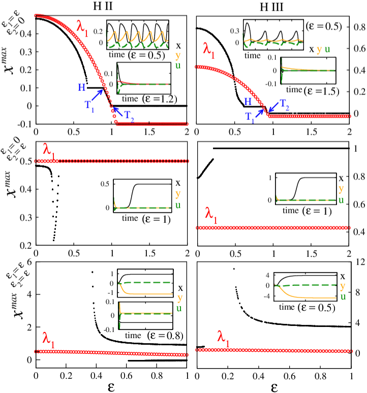
Since one of the roots $\lambda=-\gamma$ is independent of $\varepsilon$ therefore the remaining roots of this equation determine the stability of the origin. The remaining two roots are $\lambda_{\pm}=-(k-r)/2\pm\sqrt{(k+r)^{2}-4\varepsilon^{2}}/2$ out of which, $\lambda_{-}<0$, $\forall$ $\varepsilon$. It is easily verifiable that the eigenvalue $\lambda_{+}$ (which also is the largest) is positive $\forall$ $\varepsilon<\sqrt{kr}$ and crosses the zero axis at $\varepsilon^{*}=\sqrt{kr}$ leading to all negative eigenvalues and hence a stable origin. This is quite similar to the harmonic oscillator case where increasing/decreasing the value of the decay parameter $k$ could increase/decrease the threshold value of stable $\to$ unstable transition (unstable $\to$ stable in this case). Furthermore, in the large $\varepsilon$ limit, we obtain the largest eigenvalue $\lambda_{1}=-\gamma$ and therefore the origin is stable in this regime. Fig. 4: top row shows the bifurcation diagram bif and the largest eigenvalue behavior for H II (left) and III (right). The unstable $\to$ stable transition in both these systems with increasing coupling values can be seen in the figure. Although for the H III system in the regime $\varepsilon>\sqrt{rk}(=0.927,$ for $r=0.43,k=2)$, certain initial conditions lead to the trajectories escaping to infinity (not shown) which accounts for the missing dots in the bifurcation figure. Since $x$ and $y$ are population variables by definition, population models are constrained to work for non-negative values of $x$ and $y$ respectively. What we observe here is that the augmentation forces the prey populations into taking negative values which leads to a breakdown in the model constraints and the logistic function in the rate equation of $x$ leads to diverging solutions as time increases. For H II system this appears not to be the case and all considered initial conditions lead to a stable origin $\forall$ $\varepsilon>\sqrt{rk}(=1,$ for $r=0.5,k=2)$.

For $\varepsilon_{1}=0$ and $\varepsilon_{2}=\varepsilon$, i.e. only the predator populations are augmented, substituting these values in Eq. 20 give,

$$(r-\lambda)[(\gamma+\lambda)(k+\lambda)+{\varepsilon}^{2}]=0,$$ (22)

and we see that an eigenvalue $\lambda=r$ is always positive since $r>0$, and therefore this setup will never stabilize the origin. The remaining eigenvalues are $\lambda_{\pm}=-(\gamma+k)/2\pm\sqrt{(k-\gamma)+4\varepsilon^{2}}/2$. In Fig. 4: second row, for low $\varepsilon$ values, the systems exhibit periodic behavior similar to the one shown for the augmented prey case. For higher values of $\varepsilon$, both H II and H III settle on a stationary solution of the original system $(x^{*},y^{*})=(K,0)$ which we did not intent to stabilize. For this solution, the preys exist at their carrying capacity and the predators vanish. For H II and H III, the carrying capacities considered for simulations are $K=0.5$ and $K=1$ respectively, and hence the observations in Fig. 4 (middle row).

For $\varepsilon_{1}=\varepsilon_{2}=\varepsilon$, i.e. both prey and predator populations are augmented, substituting these values in Eq. 20 and rearranging terms gives,

$$\lambda^{3}+(\gamma+k-r)\lambda^{2}+(2\varepsilon^{2}+(\gamma-r)k-r\gamma)\lambda$$

$$+\varepsilon^{2}(\gamma-r)-r\gamma k=0.$$ (23)

Using the RHC Rou , one of the conditions for this equation to have all negative roots is $\varepsilon>\sqrt{\dfrac{r\gamma k}{(\gamma-r)}}$ which is impossible to achieve since $r>\gamma$. Therefore, this setup will not stabilize the origin either. Fig. 4: bottom row shows the behavior of H II and H III. For smaller $\varepsilon$ values, these systems exhibit periodic behavior similar to the augmented prey. On increasing $\varepsilon$ further, systems enter a regime where all considered initial conditions lead to escaping trajectories. The reason behind this behavior here again is due to a breakdown in modeling constraints. Examination of transient trajectories reveals that augmentation in this case is forcing the predator populations into $y<0$ axis which leads to a breakdown in the model, thereby initiating a positive feedback loop in the prey populations leading to the diverging behaviors observed in simulations. Beyond this regime for higher values of $\varepsilon$, H II system exhibits bistability between different stationary solutions where in one case, preys exceed their carrying capacity $(x^{*}>K)$ and the predator populations are negative $(y^{*}<0)$, and in the other case, the prey populations are negative $(x^{*}<0)$ and predators assume a small positive value. It is important to note yet again that these solutions are impractical because the populations cannot exist above their carrying capacities nor can they take negative values under realistic modeling constraints. For H III system, we only observe the equilibrium solutions with $x^{*}>K$ and $y^{*}<0$ (see inset). In both the cases, we have a non vanishing $u^{*}>0$ and therefore these solutions exist due to augmentation and cannot be observed otherwise. Following this analysis, we can conclude that augmenting the prey is the correct strategy to stabilize of the origin and the other coupling schemes can lead to complicated dynamics. Even though the analysis here is limited to the origin, we can expect these behaviors to be quite general with respect to other stationary solutions as well.

Figure 5: (Color online) Different dynamical regimes for H II and H III systems are marked as A, B and C in the $\varepsilon$, $k$ plane. A is the regime of periodic dynamics, in B stationary solutions of the coupled system are stable and C is the regime of stable origin. The boundaries between A$\to$B and B$\to$C are the loci of the reverse Hopf bifurcation $H$ and the second transcritical bifurcation $T_{2}$ respectively (as in Fig. 4: top row).

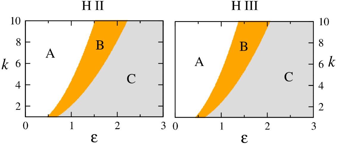
Now considering applications, as already mentioned, origin corresponds to an equilibrium for which the predators and the preys vanish. Persistence of populations for a proper ecosystem function is very imperative and has been studied extensively from several perspectives, contributing towards a better understanding of the processes leading to species extinction Lande (1993); Hanski (1999); Hughes et al. (1997); Ceballos and Ehrlich (2002); Folke et al. (2004). Knowledge regarding these processes can help in devising procedures which can contribute towards better species conservation efforts. For the simple models considered in the previous analysis, it is clear that either by coupling the system appropriately or by using specific parameter values for $k$ and $\varepsilon$, we can avoid stabilizing the origin. For instance, considering the prey augmented case, for low $\varepsilon$, the systems exhibit periodic oscillations. On increasing the coupling strength, stationary solutions of the augmented system $(x^{*}>0,y^{*}>0,u^{*}<0)$, satisfying

$$rx^{*}(1-x^{*}/K)-f(x^{*})y^{*}+\varepsilon_{1}u^{*} = 0,$$

$$(\rho f(x^{*})-\gamma)y^{*} = 0,$$

$$-ku^{*}-\varepsilon x^{*} = 0,$$ (24)

get stabilized through a reverse Hopf bifurcation (marked as $H$ in Figs. 4 (top row)). For these stationary solutions, the value of $x^{*}$ stays constant while $y^{*}$ and $u^{*}=-\varepsilon x^{*}/k$ show a variation for a range of $\varepsilon$ values (plateau between $H$ and $T_{1}$ in Fig. 4 (top row)). It is also important to note that some initial conditions in this regime can lead to trajectories escaping to infinity. This branch of solutions undergoes a transcritical bifurcation (marked $T_{1}$ in Fig. 4 (top row)) where it exchanges stability with another branch of solutions with $u^{*}\to 0$ for increasing $\varepsilon$. At $\varepsilon^{*}=\sqrt{rk}$, $u^{*}=0$ and the predator–prey system effectively decouples from augmentation which is accompanied by another transcritical bifurcation ($T_{2}$ in Fig. 4 (top row)) between the continuing branch of stationary solutions $(x^{*}>0,y^{*}>0,u^{*}\to 0)$ and the origin. In $\varepsilon>\varepsilon^{*}$ regime, origin is the only dynamical attractor. Fig. 5 shows the parameter scans for H II and H III systems highlighting these different dynamical regimes. In region A these systems exhibit periodic behavior and the boundary between A and B is the locus of the Hopf bifurcation in the $\varepsilon$, $k$ plane, which leads to the stabilization of stationary solutions $(x^{*}>0,y^{*}>0,u^{*}<0)$. B corresponds to the regime where stable stationary solutions $(x^{*}>0,y^{*}>0,u^{*}<0)$ and $(x^{*}>0,y^{*}>0,u^{*}\to 0)$ are observed and the boundary between B and C is the locus of the second transcritical bifurcation $T_{2}$ which leads to the stabilization of the origin. Therefore by using appropriate values of $\varepsilon$ and $k$, we can keep the system in either a periodic state, or a stationary state with non vanishing populations and can expect this procedure to work in experiments and be robust with respect to noise; Ref. Sharma et al. (2011) experimentally stabilized a stationary solution in an electronic Lorenz system at permitted noise level. Furthermore, in the other instances of augmented predators, or augmented predators and preys we already observe a complete lack of origin stabilization. Therefore, we can employ these schemes as well to avoid stabilizing the origin but one needs to be careful since these cases can lead to other complications as discussed. Another useful application for these observations could be in cases where maximization of prey yield is required. Augmenting the predator populations is seen to stabilize the equilibrium where the prey populations exist at their carrying capacity and the predators vanish. This can find applications in fisheries Yodzis (1994); Christensen (1996), algae fuel generation Scott et al. (2010); Oncel (2013); where maximal sustainable yields are crucial, and also in biomedical research, for e.g. in HIV-1 infection models Boer and Perelson (1998) where a portion of human immune system i.e. activated CD$4^{+}$ T cells are the primary target of the HIV-1 infection Fauci (1993); Weiss (1993) which can be modeled via predator–prey dynamics.

IV Summary

In this work we studied the general ability of linear augmentation towards stabilizing desired stationary solutions of oscillatory systems. Through some simple examples discussed in this paper, it is clear that the effectiveness of this scheme is quite sensitive to the augmentation parameters, the class of oscillatory systems considered, the stationary solutions to stabilize and also on the way the systems are augmented. Therefore, although the simplicity of linear augmentation makes it a very compelling choice for applications, a careful analysis is required to test the system for potential pitfalls associated with the scheme. As highlighted by the examples, apart from failing to target the appropriate stationary solutions, linear augmentation can also lead to other complicated dynamical situations which include escaping trajectories, stabilization of unintended stationary solutions or the stabilization of stationary solutions which are not permitted under the modeling constraints; preys existing above their carrying capacities and negative predator populations in Sec. III.3 for instance. Nevertheless, one can find ways to exploit the failures of the scheme in applications. Although we can expect to see these results in experiments, an in-depth study of this procedure in presence of noise, and also for larger systems is required. Extending on the results in the ecological context, one needs to check the process behavior in presence of multiple preys and predators, for a food chain, and also for other functional responses Karnatak . Furthermore, linear augmentation has been proposed as a mechanism to control bistability Sharma et al. (2013) but how it fares in managing more general instances of multistability including extreme multistability Ngonghala et al. (2011); Karnatak et al. (2014b) is still an open question and will be addressed in subsequent studies Karnatak .

Acknowledgment: The author would like to thank anonymous referees for their constructive comments and suggestions, A. Nandi, S. Bialonski for a critical reading of the manuscript and related discussions, and A. V. Costea for help with the text. The author acknowledges the Max Planck Society for research support.

Appendix A Converging and diverging trajectories in augmented harmonic oscillator

Figure 6: (Color online) Bifurcation diagram (black dots) along with the largest eigenvalue (red symbols) as a function of $\varepsilon$ in the top row. $\varepsilon^{*}=\omega\sqrt{\dfrac{k}{\omega^{2}-1}}(\sim 1.63)$ marks the coupling beyond which all initial conditions lead to escaping trajectories. Transient trajectories shown for $\varepsilon(=0.5)<\varepsilon^{*}$ (left bottom) and $\varepsilon(=1.75)>\varepsilon^{*}$ (right bottom).

Augmented harmonic oscillator dynamics from Eq. III.1 can also be expressed in form of a second order ODE as,

$$\mathbb{D}x=U(\varepsilon_{1},\varepsilon_{2},k,t)[=\{\varepsilon_{2}+\varepsilon_{2}{\varepsilon_{1}}^{2}-\varepsilon_{1}k\}u(t)],$$ (25)

where the derivative operator $\mathbb{D}=D^{2}+\varepsilon_{1}\varepsilon_{2}D+({\varepsilon_{1}^{2}}+\omega^{2})$ with $D^{i}=\dfrac{d^{i}}{dt^{i}}$, $i=1,2$ in this case. This equation corresponds to a driven harmonic oscillator with frequency $(\varepsilon_{1}^{2}+\omega^{2})$ and a damping coefficient $\varepsilon_{1}\varepsilon_{2}$. The roots of the auxiliary equation for the operator $\mathbb{D}$ are $m_{\pm}=\alpha\pm\beta$ where $\alpha=-{\varepsilon_{1}\varepsilon_{2}}/2$ and $\beta=\sqrt{\varepsilon_{1}^{2}\varepsilon_{2}^{2}-4(\varepsilon_{1}^{2}+\omega^{2})}/2$. For partially augmented cases $\alpha=0$ and $\beta=\sqrt{-4(\varepsilon_{1}^{2}+\omega^{2})}/2$ or $\beta=i\omega$ for $\varepsilon_{2}=0,\varepsilon_{1}\neq 0$ and $\varepsilon_{1}=0,\varepsilon_{2}\neq 0$ respectively.

For identical augmentation $\varepsilon_{1}=\varepsilon_{2}=\varepsilon$, we get $\mathbb{D}=D^{2}+\varepsilon^{2}D+(\varepsilon^{2}+\omega^{2})$ and Eq. 25 reads

$$\mathbb{D}x=U(\varepsilon,k,t)[=\varepsilon\{1+\varepsilon^{2}-k\}u(t)].$$ (26)

The roots of the auxilliary equation in this case are $m_{\pm}=\alpha\pm\beta$ with $\alpha=-{\varepsilon^{2}}/2$ and $\beta=\sqrt{\varepsilon^{4}-4(\varepsilon^{2}+\omega^{2})}/2$. For imaginary $\beta$, the transient solution for Eq. 26 can be expressed as,

$$x_{g}(t)=Ax_{1}(t)+Bx_{2}(t),$$ (27)

which is independent of the forcing term $U(\varepsilon,k,t)$ with $x_{1}(t)=\exp{(\alpha t)}\cos{\beta t}$, and $x_{2}(t)=\exp{(\alpha t)}\sin{\beta t}$. Consequently, the steady state solution can be obtained by using the Laplace and inverse Laplace transformations giving,

$$x_{st}(t)=\dfrac{1}{\Omega}\int_{0}^{t}e^{-\gamma(t-x)}\sin{(\Omega(t-x))}U(\varepsilon,k,x)dx,$$

(28)

where $\Omega=\sqrt{\omega_{0}^{2}-\gamma^{2}}$, ${\omega_{0}}^{2}=\varepsilon^{2}+\omega^{2}$ and $\gamma=\varepsilon^{2}/2$. Now at this point, we do not know the exact expression for $U(\varepsilon,k,t)$. Considering the transient behavior of trajectories in partially/fully augmented system, we clearly observe that they possess an exponentially decaying/diverging envelop (see Fig. 1 (inset) and Fig. 6 bottom row). Based on these observations, assuming $U(\varepsilon,k,t)=a_{0}\exp{(k_{m}t)}$ where both $a_{0},k_{m}$ are functions of $\varepsilon$ and $k$, and solving Eq. 28 gives

$$x_{p}(t)=\exp{(k_{m}t)}\left(\dfrac{a_{0}}{(k_{m}+\alpha)^{2}-\beta^{2}}\right).$$ (29)

From this expression we see that the trajectories will exponentially decay to the origin $\forall$ $k_{m}<0$ and diverge $\forall$ $k_{m}>0$.

Figure 7: (Color online) Largest eigenvalues and estimated values of $k_{m}$ as functions of $\varepsilon$, (a) for the system augmented in $x$ and (b) for the fully augmented system.

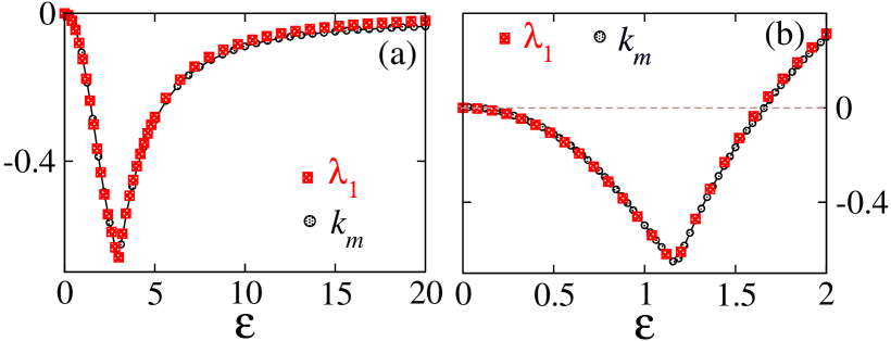
Fig. 7 shows the numerical estimation of $k_{m}$ along with the largest eigenvalue of the Jacobian $\lambda_{1}$ at the origin as a function of $\varepsilon$; for partially (Fig. 7 (a)) and fully augmented cases (Fig. 7 (b)). $k_{m}$ here was calculated as the average rate of convergence/divergence in the Euclidean distance of the current systems’ state from its previous state, for every time step along the trajectory. These results suggest that $k_{m}=\lambda_{1}$ and this observation has some interesting consequences. For $k_{m}=\lambda_{1}<0$, we have a case of a harmonic oscillator being driven by an exponentially decaying force and consequently the system settles on the origin as $t\to\infty$. Similarly the other case of an unstable origin ($k_{m}=\lambda_{1}>0$) is equivalent to the oscillator under the influence of an exponentially diverging force (energy being pumped into the system) which leads to diverging trajectories as time increases.

Appendix B Hysteresis in augmented Duffing model

Figure 8: (Color online) Maximal Lyapunov exponent for increasing and decreasing values of $\varepsilon$ for the fully augmented Duffing system with $(x^{*}=1,y^{*}=0)$ demonstrating hysteresis. Calculations for increasing and decreasing $\varepsilon$ are marked by red and black arrows respectively.

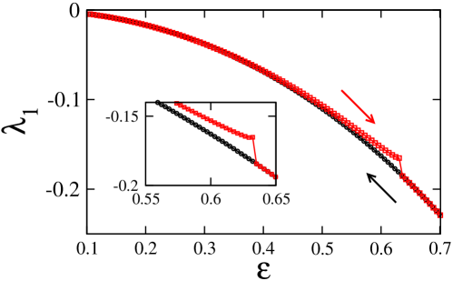
For the bistable fully identically augmented Duffing system in Eq. 8 with $x^{*}=1,y^{*}=0$, the largest Lyapunov exponent was calculated for increasing and decreasing values of augmentation strength $\varepsilon$. Starting with initial conditions leading to the solutions $({x^{*}}_{-},{y^{*}}_{-},{z^{*}}_{-})$ at $\varepsilon=0.1$, the initial conditions for the next calculation at $\varepsilon=0.1+\delta\varepsilon$ were taken as the final values of $x,y,u$ from the previous calculation for $\varepsilon=0.1$, with $\delta\varepsilon=0.001$ and so on for the entire range in the forward direction. Similarly for backwards calculation, the process was repeated starting from $\varepsilon=0.7$ where $(1,0)$ is the only stable solution with $\delta\varepsilon=-0.001$. The results of the calculation are shown in Fig. 8 and as one would expect, this system exhibits hysteresis in the interval of bistablity.

Appendix C Fully augmented Duffing system: behavior in $(\varepsilon,k)$ plane

Figure 9: (Color online) Behavior of fully augmented Duffing system in the $(\varepsilon,k)$ plane. Parameter regimes marked in grey (A) correspond to a successful stabilization of the intended stationary solution; $(1,0)$ in (a) and $(0,0)$ in (b). Regimes of bistability are marked with blue dots and B corresponds to parameter values for which other stationary solutions are stable.

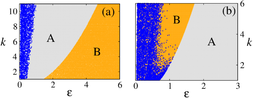
Different dynamical regimes for the Duffing system in Eq. 8 with $(x^{*},y^{*})=(1,0)$ and $(0,0)$ are shown in Fig. 9. The grey areas marked as A correspond to the regimes where the intended stationary solutions are successfully stabilized, namely $(1,0)$ and $(0,0)$ in Figs. 9(a) and (b) respectively.

For $x^{*}=1,y^{*}=0$ in Fig. 9(a): blue dots for lower $\varepsilon$ values highlight the regimes of bistability where solutions $({x^{*}}_{-},{y^{*}}_{-},{z^{*}}_{-})$ (from Eq. 13) and $(1,0)$ coexist. Solutions $({x^{*}}_{-},{y^{*}}_{-},{z^{*}}_{-})$ vanish via a saddle node bifurcation after colliding with the unstable branch of solutions $({x^{*}}_{+},{y^{*}}_{+},{z^{*}}_{+})$ (again from Eq. 13) and the boundary of the blue dot regime gives the locus of this saddle node bifurcation; parabolic function $F_{SN}(\varepsilon,k)(=5\varepsilon^{2}-k)=0$, estimated from the expression for ${x^{*}}_{\pm}$ from Eq. 13 as the limiting value of $k$ and $\varepsilon$ to get real solutions, obtained by equating the discriminant in the expression of ${x^{*}}_{\pm}$ to zero. The boundary between regimes A and B corresponds to the locus of the transcritical bifurcation between $(1,0)$ and $({x^{*}}_{+},{y^{*}}_{+},{z^{*}}_{+})$ given by the zero crossing of the largest eigenvalue for $(1,0)$ which satisfies $F_{TC}(\varepsilon,k)(=2\varepsilon^{2}-k)=0$. In region B either the now stable coupling dependent stationary solutions $({x^{*}}_{+},{y^{*}}_{+},{z^{*}}_{+})$, or escaping trajectories are observed.

Similarly for $x^{*}=0,y^{*}=0$ in Fig. 9(b): B highlights the regime where the system settles on the solutions $({x^{o}}_{+},{y^{o}}_{+},{u^{o}}_{+})$. The blue dots correspond to the initial conditions leading to stationary solutions $({x^{o}}_{-},{y^{o}}_{-},{u^{o}}_{-})$. Since the system is bistable in this regime, we should expect the entire region B to be densely filled with these blue dots but that is not the case. The reason behind this behavior is a difference in the relative basin size of these two solutions; number of initial conditions leading to $({x^{o}}_{+},{y^{o}}_{+},{u^{o}}_{+})$ is more than the ones which lead to $({x^{o}}_{-},{y^{o}}_{-},{u^{o}}_{-})$. This difference is even more pronounced for higher values of $k$. Both these solutions vanish via a pitchfork bifurcation and the locus of this bifurcation which separates regimes B and A can be traced by the function $F_{PF}(\varepsilon,k)(=2\varepsilon^{2}-k)=0$ which is obtained by equating the discriminant in the expression of ${x^{o}}_{\pm}$ from Eq. 16 to zero.

References

- Pikovsky et al. (2001) A. Pikovsky, M. Rosenblum, and J. Kurths, Synchronization: A Universal Concept in Nonlinear Sciences (Cambridge University Press, 2001).
- Saxena et al. (2012) G. Saxena, A. Prasad, and R. Ramaswamy, Physics Reports 521, 205 (2012), and references therein.
- Koseska et al. (2013) A. Koseska, E. Volkov, and J. Kurths, Physics Reports 531, 173 (2013), and references therein.
- Feudel (2008) U. Feudel, International Journal of Bifurcation and Chaos 18, 1607 (2008).
- Prasad et al. (2005) A. Prasad, L. D. Iasemidis, S. Sabesan, and K. Tsakalis, Pramana 64, 513 (2005).
- Ansmann et al. (2013) G. Ansmann, R. Karnatak, K. Lehnertz, and U. Feudel, Physical Review E 88, 052911 (2013).
- Karnatak et al. (2014a) R. Karnatak, G. Ansmann, U. Feudel, and K. Lehnertz, Physical Review E 90, 022917 (2014a).
- Schöll and Schuster (2008) E. Schöll and H. G. Schuster, Handbook of chaos control (John Wiley & Sons, 2008).
- Ott et al. (1990) E. Ott, C. Grebogi, and J. A. Yorke, Phys. Rev. Lett. 64, 1196 (1990).
- Pecora and Carroll (1990) L. M. Pecora and T. L. Carroll, Phys. Rev. Lett. 64, 821 (1990).
- Pyragas (1992) K. Pyragas, Physics Letters A 170, 421 (1992).
- Peng et al. (1996) J. H. Peng, E. J. Ding, M. Ding, and W. Yang, Phys. Rev. Lett. 76, 904 (1996).
- Pisarchik and Feudel (2014) A. N. Pisarchik and U. Feudel, Physics Reports 540, 167 (2014), and references therein.
- Gang and Zhilin (1994) H. Gang and Q. Zhilin, Phys. Rev. Lett. 72, 68 (1994).
- Boccaletti et al. (1999) S. Boccaletti, J. Bragard, and F. T. Arecchi, Phys. Rev. E 59, 6574 (1999).
- Balanov et al. (2004) A. Balanov, N. Janson, and E. Schöll, Physica D: Nonlinear Phenomena 199, 1 (2004).
- Hauschildt et al. (2006) B. Hauschildt, N. B. Janson, A. Balanov, and E. Schöll, Phys. Rev. E 74, 051906 (2006).
- Bar-Eli (1984) K. Bar-Eli, Journal of Physical Chemistry 88, 3616 (1984).
- Ermentrout (1990) G. Ermentrout, Physica D: Nonlinear Phenomena 41, 219 (1990).
- Aronson et al. (1990) D. Aronson, G. Ermentrout, and N. Kopell, Physica D: Nonlinear Phenomena 41, 403 (1990).
- Mirollo and Strogatz (1990) R. Mirollo and S. Strogatz, Journal of Statistical Physics 60, 245 (1990).
- Ramana Reddy et al. (1998) D. Ramana Reddy, A. Sen, and G. Johnston, Phys. Rev. Lett. 80, 5109 (1998).
- Atay (2003) F. Atay, Phys. Rev. Lett. 91, 941011 (2003).
- Karnatak et al. (2007) R. Karnatak, R. Ramaswamy, and A. Prasad, Phys. Rev. E 76, 035201 (2007).
- Konishi (2003) K. Konishi, Phys. Rev. E. 68, 672021 (2003).
- Sharma et al. (2011) P. R. Sharma, A. Sharma, M. D. Shrimali, and A. Prasad, Phys. Rev. E 83, 067201 (2011).
- Sharma et al. (2013) P. R. Sharma, M. D. Shrimali, A. Prasad, and U. Feudel, Phys. Lett. A 377, 2329 (2013).
- Sharma et al. (2014) P. R. Sharma, A. Singh, A. Prasad, and M. D. Shrimali, The European Physical Journal Special Topics 223, 1531 (2014).
- Sharma et al. (2015) P. R. Sharma, M. Shrimali, A. Prasad, N. V. Kuznetsov, and G. A. Lenov, International Journal of Bifurcation and Chaos 25, 1550061 (2015).
- Resmi et al. (2010) V. Resmi, G. Ambika, and R. E. Amritkar, Phys. Rev. E 81, 046216 (2010).
- (31) The system is evolved for 10 different initial condition for each value of the control parameter sufficiently for the transients to be discarded. System is then further evolved to capture the dynamical regimes in the system by noting all possible extrema in the dynamics for the duration of evolution.
- (32) Given a polynomial , where the coefficients ’s are real, then all roots of the polynomial are negative or have negative real parts iff the determinants of all Hurwitz matrices are positive. For , this occurs when the coefficients and are strictly positive and .
- (33) For any general cubic equation , the discriminant is defined as .
- Solomon (1949) M. E. Solomon, Journal of Animal Ecology 18, 1 (1949).
- Holling (1959a) C. S. Holling, The Canadian Entomologist 91, 293 (1959a).
- Holling (1959b) C. S. Holling, The Canadian Entomologist 91, 385 (1959b).
- Lotka (1910) A. J. Lotka, The Journal of Physical Chemistry 14, 271 (1910).
- Volterra (1926) V. Volterra, Nature 118, 558 (1926).
- Rosenzweig and MacArthur (1963) M. L. Rosenzweig and R. H. MacArthur, The American Naturalist 97, 209 (1963).
- Truscott and Brindley (1994) J. Truscott and J. Brindley, Philosophical Transactions of the Royal Society of London. Series A: Physical and Engineering Sciences 347, 703 (1994).
- de Roos (2013) A. M. de Roos, Modeling Population Dynamics (available online on the authors webpage at https://staff.fnwi.uva.nl/a.m.deroos, 2013).
- Karnatak et al. (2014b) R. Karnatak, R. Ramaswamy, and U. Feudel, Chaos, Solitons & Fractals 68, 48 (2014b).
- Lande (1993) R. Lande, The American Naturalist 142, 911 (1993).
- Hanski (1999) I. Hanski, Metapopulation Ecology, Oxford series in ecology and evolution (Oxford University Press, 1999).
- Hughes et al. (1997) J. B. Hughes, G. C. Daily, and P. R. Ehrlich, Science 278, 689 (1997).
- Ceballos and Ehrlich (2002) G. Ceballos and P. R. Ehrlich, Science 296, 904 (2002).
- Folke et al. (2004) C. Folke, S. Carpenter, B. Walker, M. Scheffer, T. Elmqvist, L. Gunderson, and C. S. Holling, Annual Review of Ecology, Evolution, and Systematics 35, pp. 557 (2004), and references therein.
- Yodzis (1994) P. Yodzis, Ecological Applications 4, 51 (1994).
- Christensen (1996) V. Christensen, Reviews in Fish Biology and Fisheries 6, 417 (1996).
- Scott et al. (2010) S. A. Scott, M. P. Davey, J. S. Dennis, I. Horst, C. J. Howe, D. J. Lea-Smith, and A. G. Smith, Current Opinion in Biotechnology 21, 277 (2010).
- Oncel (2013) S. S. Oncel, Renewable and Sustainable Energy Reviews 26, 241 (2013).
- Boer and Perelson (1998) R. J. D. Boer and A. S. Perelson, Journal of theoretical Biology 190, 201 (1998).
- Fauci (1993) A. Fauci, Science 262, 1011 (1993).
- Weiss (1993) R. Weiss, Science 260, 1273 (1993).
- (55) R. Karnatak, In preparation.
- Ngonghala et al. (2011) C. Ngonghala, U. Feudel, and K. Showalter, Phys. Rev. E 83, 056206 (2011).