Optimal Cell Clustering and Activation for Energy Saving in Load-Coupled Wireless Networks

Abstract

Optimizing activation and deactivation of base station transmissions provides an instrument for improving energy efficiency in cellular networks. In this paper, we study the problem of performing cell clustering and setting the activation time of each cluster, with the objective of minimizing the sum energy, subject to a time constraint of serving the users’ traffic demand. Our optimization framework accounts for inter-cell interference, and, thus, the users’ achievable rates depend on cluster formation. We provide mathematical formulations and analysis, and prove the problem’s NP hardness. For problem solution, we first apply an optimization method that successively augments the set of variables under consideration, with the capability of approaching global optimum. Then, we derive a second solution algorithm to deal with the the trade-off between optimality and the combinatorial nature of cluster formation. Numerical results demonstrate that our solutions achieve more than 40% energy saving over existing schemes, and that the solutions we obtain are within a few percent of deviation from global optimum.

I Introduction

Energy efficiency has become a major concern for cellular networks due to the explosive growth of data traffic. Among the system elements, base stations (BSs) account for more than $80\%$ of the total energy consumption [1], calling for new approaches for BS operation. To this end, one solution is to coordinate and optimize the activities of BSs, and the paradigm of BSs operation has been shifted from “always on” to “always available” [2]. Some underutilized BSs with low traffic can be turned off, for example, to reduce the energy consumption, if the data traffic of the BSs can be offloaded to other BSs. Another related scheme for energy saving is to organize the BSs by clusters such that one cluster is active at a time. The cells within a cluster are in transmission if and only if the cluster is active. In this paper, we optimize cell cluster formation and the activation time duration of each cluster, with energy as the performance metric.

I-A Related Works

There are a number of studies that consider energy saving by deactivating BSs [3, 4, 5]. In these works, the periodic nature of cell’s traffic, both temporally and spatially, is exploited. Energy consumption is reduced by deactivating some BSs when the traffic demand is low. If a BS is deactivated, its service coverage is taken care of by other neighboring BSs that remain active. Coordinated Multi-Point (CoMP) transmission can be applied, see e.g., [6], to avoid coverage holes.

Energy saving can also be gained by deactivating BSs’ power amplifiers (PAs) if the amount of traffic does not require fully continuous transmission. In the transmission mode, the PAs are accounted for most of the energy consumption. Typically, 50-80% of the total energy of a BS is consumed by the PAs [1]. For long term evolution (LTE) systems, deactivating the PAs can be done by adopting discontinuous transmission (DTX) at the BSs, implemented by the use of Almost Blank Subframe (ABS) [7]. In [8], performance evaluation of DTX is carried out for a realistic traffic scenario.

In BS scheduling, the BSs are grouped into clusters that potentially can overlap, such that one cluster is active (i.e., used for transmission) at a time, and a schedule is designed to optimize the use of clusters to serve the user demand with minimum energy. In [2], the authors assessed the performance of coordinated scheduling of BS activation. In this case, inter-BS coordination is carried out for groups of three cells, with pre-defined and fixed deactivation period of each BS. In [9], the authors proposed a coordinated activation scheme, in which the BSs are split into multiple BS groups. For each group, the BSs switch between activation and deactivation according to a pre-defined pattern. Simulation results in [9] show that the scheme leads to 40% less energy consumption. In [10], the authors considered four BS deactivation patterns, to allow for progressively deactivating BSs to improve energy efficiency, while maintaining the quality of service (QoS). Energy saving is achieved by dynamically selecting the four patterns adaptively depending on the traffic demand.

Another related topic is transmission scheduling in wireless ad hoc and mesh networks (see, e.g., [11, 12], and the references therein). The task is to organize links into groups, and determine the number of time slots assigned to each group, in order to meet the demand with minimum time (a.k.a. minimum-length scheduling). A subset of links can form a group if and only if the signal-to-interference-and-noise ratio (SINR) at the receivers meets a given threshold. A problem generalization to continuous rates is studied in [13]. In [14], the authors studied transmission scheduling in mesh networks with a performance metric that weights together time and energy.

I-B Our Work

Most of the previous works for coordinated BS activation focus on saving energy enabled by scenarios with relatively low user demand. For the more general scenario with no specific assumption on user demand level, energy-optimal BS scheduling for delivering the demand within a strict time limit is challenging, due to the fact that the achievable transmission rates within each cell are constrained by the inter-cell interference. For LTE networks, the transmission rates (i.e., demand delivered per time unit) in different cells are inherently coupled with each other due to mutual interference. To characterize the achievable rates, we adopt the coupling model in [15, 16, 17, 18] for cell load-dependent SINR. Here, cell load refers to the utilization level of the time-spectrum resource units (RUs) in orthogonal frequency division multiple access (OFDMA). The cell load levels are coupled, i.e., they influence each other. Namely, because the load reflects the amount of use of RUs for transmission, the inter-cell interference generated by a cell to another cell depends on the load of the former, and the interference, in its turn, has impact on the load level of the latter. In the load-coupling model, the dependency relation of the cell load levels is taken into account in the SINR computation. To the best of our knowledge, energy-efficient BS clustering and scheduling, subject to maximum delay and rate characterization based on the coupling relation among cells, has not been investigated in the literature.

In this paper, we formulate, analyze, and solve energy-efficient cell clustering and scheduling (CCS), where the cells are required to serve a target amount of data for the users within a time limit to maintain an appropriate level of QoS, while considering the coupling relation among cells due to interference. Each cluster is a subset of cells that are in simultaneous transmission mode, when the cluster is active. Instead of pre-defined clusters, in CCS cell clustering as well as cluster activation times are optimized. Within a cell, the achievable rate vectors for the cell’s users, taking into account inter-cell interference, is not unique but form a rate region. Thus solving CCS also involves the selection of rate vectors.

We present the following contributions. First, we formulate CCS and prove its NP-hardness. A problem is called non-deterministic polynomial-time hard, or NP-hard in short, if it is at least as difficult as a large class of computational problems referred to as NP, and, thus far, no polynomial-time algorithms exist for NP-hard problems. As the next contribution, we present and prove a theoretical result to enable to confine the consideration of rate vectors to a finite set without loss of optimality. On the algorithmic side, we show how column generation [19, 20, 12] facilitates problem solving, and thereby derive an algorithm for optimal cell clustering and scheduling (AOCCS) to approach the global optimum. Column generation is an optimization method, in which a mathematical model is successively expanded with new variables, such that the objective function gets improved after each expansion, until the global optimum is reached. By our complexity results of computational intractability, for large networks solving CCS optimally is challenging. We then introduce our notion of locally enumerating interference, that is, for each BS, the rate evaluation of its users considers a selected small set of nearby BSs as sources of interference, utilizing the fact that interference from distant BSs is insignificant. Using this notion, we present a local-enumeration-based bounding scheme (LEBS), providing lower and upper bounds on the global optimum of minimum energy, as well as enabling to deal with the trade-off between optimality and the combinatorial nature of cluster formation. The bounds, in turn, serve the purpose of gauging the deviation from optimality. Moreover, from LEBS, we derive a near-optimal cluster scheduling approach (NCSA). We present numerical results to illustrate the performance of the proposed approaches. The results show significant energy savings by AOCCS, and the near optimality of solutions enabled by LEBS and NCSA. We remark that, even though regular, hexagon-shaped cells are used for performance evaluation for the purpose of comparative study, our system model and the optimization approaches do not impose any topological assumption, and hence they are generally applicable to any given cellular network layout.

The rest of the paper is organized as follows. Section II gives the system model. In Section III, we formulate CCS and prove its complexity. Section IV presents algorithm AOCCS. Section V details the LEBS scheme and NCSA. Numerical results are given in Section VI. Section VII concludes the paper.

Notations: We denote a (tall) vector by a bold lower case letter, say $\bm{a}$, a matrix by a bold capital letter, say $\bm{A}$. A set is denoted by a letter in calligraphic style, say ${\mathcal{A}}$. Notation $\prec$ and $\preceq$ are for componentwise inequalities between vectors.

II System Model

II-A Cellular Network with Cell Coupling

Consider a downlink OFDMA based cellular network with $I$ BSs serving $J$ users. We use ${\mathcal{I}}=\{1,\dots,I\}$ and ${\mathcal{J}}=\{1,\dots,J\}$ to denote the sets of BSs and users, respectively. The set of users of BS $i$ is denoted by ${\mathcal{J}}_{i}$, and user sets of all BSs form a partitioning of ${\mathcal{J}}$. Let $J_{i}=|{\mathcal{J}}_{i}|$, we have $\sum_{i\in{\mathcal{I}}}J_{i}=J$. Throughout the paper, we refer to BS $i$ interchangeably with cell $i$. In OFDMA, the time-frequency domain resource is divided into resource units (RUs). A cell serves its users by orthogonal (i.e., non-overlapping) use of the RUs. We use $d_{ij}$ to denote the traffic demand (in bits) of user $j$ in cell $i$. As a QoS requirement, all users’ demands have to be served within time $T$.

In the load-coupling model, the SINR computation over one RU uses the cell load levels to take into account inter-cell interference. In the following, we derive the SINR of one RU for user $j$ of BS $i$. We denote by $p_{i}$ the transmission power per RU of cell $i$, and $g_{ij}$ the channel gain. The noise effect is denoted by $\eta$, which equals the power spectral density of white Gaussian noise times the bandwidth of a RU. For inter-cell interference from another BS $k$ ($k\not=i$), we use $p_{k}$ and $g_{kj}$ to denote the corresponding transmission power and channel gain with respect to user $j$. Note that interference is zero if BS $k$ is not utilizing any resource. Following [15, 16, 17, 18], we use the resource utilization level of BS $k$ as a scaling factor in interference modeling. With the given notation and discussion, the SINR of user $j$ in cell $i$ is formulated below.

$${\text{SINR}}_{ij}=\frac{p_{i}g_{ij}}{\sum_{k\in{\mathcal{I}}\backslash\{i\}}p_{k}g_{kj}l_{k}+\eta}$$ (1)

In (1), entity $l_{k}$ is referred to as cell load, and denotes the utilization level of RUs in cell $k$, that is, the proportion of RUs allocated for transmission. The load vector is denoted by ${\bm{l}}=[l_{1},\dots,l_{i},\dots,l_{I}]^{T}$. In [18], it is shown that utilizing resource fully, i.e., ${\bm{l}}={\bm{1}}$ is optimal from an energy standpoint. However, operating at full load means there is no spare OFDMA resource units. For the sake of generality, our system model is formulated for any preferred load level, with ${\bm{0}}\prec{\bm{l}}\preceq{\bm{1}}$. Note that in (1), the product $p_{k}g_{kj}l_{k}$ represents the amount of the interference from cell $k$ to user $j$. The interference is Gaussian distributed in the worst case. Therefore, by using Gaussian code, the achievable rate, in bits per second, for user $j$ on one RU with bandwidth $B$ is computed as $B\log_{2}(1+\mathrm{SINR}_{ij})$, where $B$ is the RU bandwidth. Therefore, to deliver a rate of $r_{ij}$ to user $j$ of cell $i$, $\frac{r_{ij}}{B\log_{2}(1+{\text{SINR}}_{ij})}$ RUs are required. Let $W$ denote the total number of RUs per cell. The corresponding load, i.e., the proportion of the RU consumption of cell $i$ due to serving user $j$, is thus $l_{ij}=\frac{r_{ij}}{WB\log_{2}(1+{\text{SINR}}_{ij})}$. Observing that $l_{i}=\sum_{j\in\mathcal{J}_{i}}l_{ij}$ for cell $i$ gives the following equation.

$$l_{i}=\sum_{j\in{\mathcal{J}}_{i}}\frac{r_{ij}}{WB\log_{2}(1+\frac{p_{i}g_{ij}}{\sum_{k\in{\mathcal{I}}\backslash\{i\}}p_{k}g_{kj}l_{k}+\eta})},\ \forall i\in{\mathcal{I}}$$ (2)

Without loss of generality, for convenience we normalize such that $WB=1$. From (2), one can observe that the users’ rates cannot be set independently from each other. Moreover, to satisfy the QoS requirement, the rate values have to be chosen such that the demand is delivered within time $T$ for all the users, that is, $Tr_{ij}\geq d_{ij},\forall j\in{\mathcal{J}}_{i},\forall i\in{\mathcal{I}}$.

II-B Multi-Cell Clustering

In Section II-A, we have given the basic elements of the system model assuming that all cells are in transmission mode. This may very well be feasible in meeting the QoS requirement, i.e., one can find rates for (2) such that all demands are delivered within time $T$. The strategy, however, may not be energy-optimal. We now consider multi-cell clustering for energy optimization. A cluster refers to a subset of ${\mathcal{I}}$, such that the BSs in the subset are either all activated or all deactivated. For all possible $2^{I}-1$ non-empty subsets of ${\mathcal{I}}$, denote by ${\mathcal{S}}$ the index set: ${\mathcal{S}}=\{1,\dots,2^{I}-1\}$. Each index $s\in{\mathcal{S}}$ maps to a unique subset of BSs. Let ${\mathcal{I}}_{s}$ denote the corresponding set of cells of element $s\in{\mathcal{S}}$. Scheduling cluster $s$ means that all the BSs in set ${\mathcal{I}}_{s}$ are activated to be in transmission mode to serve their associated users, whereas all the BSs in ${\mathcal{I}}\setminus{\mathcal{I}}_{s}$ are deactivated. In the latter case, the BS radio components are turned off and no data can be transmitted. There is a transition time between activation and deactivation modes [8]. The transition time is however much smaller than the entire scheduling period [7], and hence we consider the transition time to be zero in this paper.

Consider a cluster $s$ with BS set ${\mathcal{I}}_{s}$. The equation (2) for cell $i\in{\mathcal{I}}_{s}$ takes the following form.

$${l_{i}=\sum_{j\in{\mathcal{J}}_{i}}\frac{r_{ij}^{s}}{\log_{2}(1+\frac{p_{i}g_{ij}}{\sum_{k\in{\mathcal{I}}_{s}\backslash\{i\}}p_{k}g_{kj}l_{k}+\eta})},\hskip 5.69046pt\forall i\in{\mathcal{I}}_{s},\leavevmode\nobreak\ \forall s\in{\mathcal{S}}}$$ (3)

Here, $r_{ij}^{s}$ represents the rate allocated to user $j$ in cell $i$ within cluster $s$. As $l_{i}$ represents a preferred resource utilization level of BS $i$, in this paper it is set independently of cell clustering. Note that in (3), the user rates are the variables. By inspecting (3), we observe that it forms a linear equation system of the user rates. We introduce the following entity.

$$b_{ij}^{s}=\frac{1}{\log_{2}(1+\frac{p_{i}g_{ij}}{\sum_{k\in{\mathcal{I}}_{s}\backslash\{i\}}p_{k}g_{kj}l_{k}+\eta})},\forall j\in{\mathcal{J}}_{i},\forall i\in{\mathcal{I}}_{s},\forall s\in{\mathcal{S}}$$ (4)

Then (3) is simplified to the equation below.

$$l_{i}=\sum_{j\in{\mathcal{J}}_{i}}b_{ij}^{s}r_{ij}^{s},\leavevmode\nobreak\ \leavevmode\nobreak\ \leavevmode\nobreak\ \leavevmode\nobreak\ \leavevmode\nobreak\ \forall i\in{\mathcal{I}}_{s},\forall s\in{\mathcal{S}}$$ (5)

For each cell $i$, its users are served when cell $i$ is active. Thus, as we assume there is at least one user per cell, every cell must be activated at least once, or, to be precise, every cell must be included in at least one cluster that has positive activation time. Note that a cell may be in multiple and active clusters. For these clusters, the achieved rates of the cell’s users and the time durations of the clusters together determine the amount of served traffic, which must meet the individual demand requirement within the specified time limit.

We would like to point out that the system model focuses on downlink. To support the downlink, some control traffic is necessary in the uplink. This can be implemented by using time division duplex (TDD) or frequency division duplex (FDD), as defined in 3GPP.

• For any cell $i\in{\mathcal{I}}_{s}$, there are infinitely many rate allocations satisfying (5). Thus one can choose to activate a cluster multiple times but with different rate allocations. In our system model, only one rate allocation is to be selected for each cluster. However, as will be clear later on, this seemingly strong restriction does not impose any loss of generality. $\Box$

III The Energy Minimization Problem

III-A Problem Formulation

Energy-efficient CCS consists of determining the clusters that shall be activated and the respective activation durations, and the optimal user rate allocation within each cluster, such that the sum energy is minimum and the users’ demand are met within the time limit. For power consumption, we adopt a model that has been widely used (e.g., [8, 21, 22]). The power of an active BS $i$ equals $p_{i}^{tot}=p_{0}+l_{i}Wp_{i}$. The first component $p_{0}$ is load-independent to account for the auxiliary power consumption due to processing circuits and cooling. The second component represents the transmission power with respect to the resource usage of BS $i$. For an inactive BS, the power consumption is considered negligibly small and assumed to be zero. Thus the power consumption of cluster $s$ is $p_{s}=\sum_{i\in{\mathcal{I}}_{s}}p_{i}^{tot}$. In the following we formally define the variables and formulate the CCS problem.

In $P1$, the objective function (6a) expresses the sum energy, by taking the product of the sum power of each cluster and its scheduled time duration. The QoS constraints (6b) and (6c) are imposed to ensure that the required demand is delivered within the time limit. Note that $i$ is not a running index in the left-hand side of (6b). The use of $i$ in the subscript of the summation is to exclude clusters that do not contain cell $i$. Here, “:” means “such that” in an optimization problem formulation. Equations (6d) define the rate region.

$$\begin{array}[]{ll}\vspace{-1.2cm}\\[10.00002pt] x_{s}&=\textrm{The time duration of activating the BSs in cluster $s$}.\\[10.00002pt] r_{ij}^{s}&=\textrm{The rate allocated to user $j$ of cell $i\in{\mathcal{I}}_{s}$, $s\in{\mathcal{S}}$.}\end{array}$$

$$P1:\leavevmode\nobreak\ \leavevmode\nobreak\ \min\leavevmode\nobreak\ \leavevmode\nobreak\ \sum_{s\in{\mathcal{S}}}p_{s}x_{s}$$ (6a)

s. t. $$\sum_{s\in{\mathcal{S}}:i\in{\mathcal{I}}_{s}}x_{s}r_{ij}^{s}\geq d_{ij},\leavevmode\nobreak\ \leavevmode\nobreak\ \forall j\in{\mathcal{J}}_{i},\leavevmode\nobreak\ \forall i\in{\mathcal{I}}$$ (6b)

$$\sum_{s\in{\mathcal{S}}}x_{s}\leq T$$ (6c)

$$\sum_{j\in{\mathcal{J}}_{i}}b_{ij}^{s}r_{ij}^{s}=l_{i},\leavevmode\nobreak\ \leavevmode\nobreak\ \leavevmode\nobreak\ \forall i\in{\mathcal{I}}_{s},\leavevmode\nobreak\ \forall s\in{\mathcal{S}}$$ (6d)

$$x_{s}\geq 0,\leavevmode\nobreak\ \leavevmode\nobreak\ \forall s\in{\mathcal{S}}$$ (6e)

We collect the user rate variables $r_{ij}^{s}$ and their coefficients $b_{ij}^{s}$ of cell $i$ in cluster $s$ as column vectors ${\bm{r}}_{i}^{s}$ and ${\bm{b}}_{i}^{s}$, respectively. Then (6d) has the following compact form.

$$({{\bm{b}}_{i}^{s}})^{T}{\bm{r}}_{i}^{s}=l_{i},\leavevmode\nobreak\ \forall i\in{\mathcal{I}}_{s},\leavevmode\nobreak\ \forall s\in{\mathcal{S}}$$ (7)

We note that (7) defines a simplex, which is a special type of $J_{i}$-dimensional polytope, as the rate region of users of cell $i$ in cluster $s$. Any point of this polytope represents an achievable rate vector, and vice versa. We use ${\mathcal{R}}_{i}^{s}$ to denote the simplex for cell $i\in{\mathcal{I}}_{s}$ in cluster $s$.

Formulation $P1$ is non-linear and non-convex, due to the product in (6b). From the discussion above, in general there are infinitely many possible rate vectors. However, we will show this non-linearity can be overcome without loss of optimality.

• From (6), the cell clustering problem is more general than BS partitioning. At optimum of CCS, a cell may be in multiple active clusters with different time durations. $\Box$

III-B Linear Formulation of CCS

Our first result is provided in Lemma 1 and Theorem 2. The result enables $P1$ to be transformed to a linear but equivalent form with a finite number of rate allocations.

Lemma 1.

Any solution to Problem $P1$ can be equivalently represented using a finite number of rate vectors.

Proof:

For any cluster $s$ and cell $i\in{\mathcal{I}}_{s}$, the simplex, denoted by ${\mathcal{R}}_{i}^{s}$, is defined in (7). Without loss of generality, suppose the user indices of an arbitrary cell $i\in{\mathcal{I}}_{s}$ is $1,\dots,J_{i}$, and ${\mathcal{I}}_{s}$ = $\{1,\dots,|{\mathcal{I}}_{s}|\}$. Simplex ${\mathcal{R}}_{i}^{s}$ has exactly $J_{i}$ vertices ${\bm{r}}_{i}^{s,1},\dots,{\bm{r}}_{i}^{s,J_{i}}$, where ${\bm{r}}_{i}^{s,j}$ is the column vector having $\frac{l_{i}}{b_{ij}^{s}}$ as its $j$th element and zero for all the other $J_{i}-1$ elements. Because ${\mathcal{R}}_{i}^{s}$ is a convex set, any vector ${\bm{r}}_{i}^{s}\in{\mathcal{R}}_{i}^{s}$ can be represented as a convex combination of ${\bm{r}}_{i}^{s,1},\dots,{\bm{r}}_{i}^{s,J_{i}}$, that is, there exist scalars $\theta_{j}\geq 0,\ j=1,\dots,J_{i}$, such that ${\bm{r}}_{i}^{s}=\theta_{1}{\bm{r}}_{i}^{s,1}+\theta_{2}{\bm{r}}_{i}^{s,2}+\dots+\theta_{J_{i}}{\bm{r}}_{i}^{s,J_{i}}$, and $\sum_{j=1}^{J_{i}}\theta_{j}=1$.

Suppose cluster $s$ is activated with time duration $x_{s}$ and rate vectors ${\bm{r}}_{i}^{s}$, $i\in{\mathcal{I}}_{s}$. For cell $i$, the vector of the amount of served user demand is given by multiplying scalar $x_{s}$ with the rate vector of this cell, i.e., $x_{s}{\bm{r}}_{i}^{s}$. By the observation above, ${\bm{r}}_{i}^{s}=\sum_{j\in{\mathcal{J}}_{i}}\theta_{j}{\bm{r}}_{i}^{s,j}$. Hence, $x_{s}{\bm{r}}_{i}^{s}=\sum_{j\in{\mathcal{J}}_{i}}x_{s}\theta_{j}{\bm{r}}_{i}^{s,j}=x_{s}\theta_{1}[\underbrace{\frac{l_{i}}{b_{i1}^{s}},0,\dots,0}_{{\bm{r}}_{i}^{s,1}}]^{T}+\dots+x_{s}\theta_{J_{i}}[\underbrace{0,\dots,0,\frac{l_{i}}{b_{iJ_{i}}^{s}}}_{{\bm{r}}_{i}^{s,J_{i}}}]^{T}$. By this substitution, $x_{s}{\bm{r}}_{i}^{s}$ is equivalently expressed by a weighted sum of rate vectors, each of which has one non-zero rate value.

For cluster $s$, denote by ${\bm{r}}^{s}$ the column vector obtained by stacking ${\bm{r}}_{1}^{s},\dots,{\bm{r}}_{|{\mathcal{I}}_{s}|}^{s}$, i.e., ${\bm{r}}^{s}=[({\bm{r}}_{1}^{s})^{T},\dots,({\bm{r}}_{|{\mathcal{I}}_{s}|}^{s})^{T}]^{T}$. Activating cluster $s$ with time duration $x_{s}$ (which is a scalar), the amount of served user demand of the cluster, in vector form, is $x_{s}{\bm{r}}^{s}=[x_{s}({\bm{r}}_{1}^{s})^{T},\dots,x_{s}({\bm{r}}_{i}^{s})^{T},\dots,x_{s}({\bm{r}}_{|{\mathcal{I}}_{s}|}^{s})^{T}]^{T}$. Applying the substitution step ${\bm{r}}_{i}^{s}=\sum_{j\in{\mathcal{J}}_{i}}\theta_{j}{\bm{r}}_{i}^{s,j}$, and observing that $\sum_{j\in{\mathcal{J}}_{i}}\theta_{j}=1$, we obtain $x_{s}{\bm{r}}^{s}=\theta_{1}[x_{s}({\bm{r}}_{1}^{s})^{T},\dots,x_{s}({\bm{r}}_{i}^{s,1})^{T},\dots,x_{s}({\bm{r}}_{|{\mathcal{I}}_{s}|}^{s})^{T}]^{T}+$ $,\dots,+\theta_{J_{i}}[x_{s}({\bm{r}}_{1}^{s})^{T},\dots,x_{s}({\bm{r}}_{i}^{s,J_{i}})^{T},\dots,\\ x_{s}({\bm{r}}_{|{\mathcal{I}}_{s}|}^{s})^{T}]^{T}$. Then, repeating the substitution procedure for the other cells leads to the conclusion that the effect of activating cluster $s$ with any rate vector ${\bm{r}}^{s}$ can be equivalently achieved by combining at most $\Pi_{i\in{\mathcal{I}}_{s}}J_{i}$ different rate vectors, and the lemma follows. ∎

• Lemma 1 further sheds light on the remark of Section III-A. Consider a solution in which a cluster is activated multiple times with different rate allocations. Because each of them is equivalent to a combination of the rate vectors from the same finite set, the activations can be aggregated into one activation, for which the rate allocation is derived from the coefficients used in the combinations. Therefore considering one rate allocation per cluster in problem formulation $P1$ does not cause any loss of generality. $\Box$

$$\bm{A}^{s}=\left[\begin{array}[]{ccccccccc}\frac{l_{i}}{b_{i1}^{s}}&\frac{l_{i}}{b_{i1}^{s}}&\frac{l_{i}}{b_{i1}^{s}}&0&0&0&0&0&0\\ 0&0&0&\frac{l_{i}}{b_{i2}^{s}}&\frac{l_{i}}{b_{i2}^{s}}&\frac{l_{i}}{b_{i2}^{s}}&0&0&0\\ 0&0&0&0&0&0&\frac{l_{i}}{b_{i3}^{s}}&\frac{l_{i}}{b_{i3}^{s}}&\frac{l_{i}}{b_{i3}^{s}}\\ \frac{l_{k}}{b_{k4}^{s}}&0&0&\frac{l_{k}}{b_{k4}^{s}}&0&0&\frac{l_{k}}{b_{k4}^{s}}&0&0\\ 0&\frac{l_{k}}{b_{k5}^{s}}&0&0&\frac{l_{k}}{b_{k5}^{s}}&0&0&\frac{l_{k}}{b_{k5}^{s}}&0\\ 0&0&\frac{l_{k}}{b_{k6}^{s}}&0&0&\frac{l_{k}}{b_{k6}^{s}}&0&0&\frac{l_{k}}{b_{k6}^{s}}\\ \end{array}\right]$$ (8)

Let ${\bm{v}}_{i}^{s}$ denote the set of vertices of ${\mathcal{R}}_{i}^{s}$. Collecting one element of each ${\bm{v}}_{i}^{s}$, $i\in{\mathcal{I}}_{s}$, leads to a column vector representing a rate allocation, in which exactly one of the users in every cell has positive rate. Enumerating all such combinations amounts to taking the Cartesian product of sets ${\bm{v}}_{i}$, $\forall i\in{\mathcal{I}}_{s}$. This gives in total $\Pi_{i\in{\mathcal{I}}_{s}}J_{i}$ rate vectors, which we index by ${\mathcal{C}}_{s}=\{1,\dots,\Pi_{i\in{\mathcal{I}}_{s}}J_{i}\}$. As an example, consider a cluster $s$ of two cells ${\mathcal{I}}_{s}=\{i,k\}$ with three users in each cell: ${\mathcal{J}}_{i}=\{1,2,3\}$ and ${\mathcal{J}}_{k}=\{4,5,6\}$. The corresponding rate vectors in ${\mathcal{C}}_{s}$ can be expressed by a $\sum_{i\in{\mathcal{I}}_{s}}J_{i}$-by-$|{\mathcal{C}}_{s}|$ matrix ${\bm{A}^{s}}$, where $\sum_{i\in{\mathcal{I}}_{s}}J_{i}=6$ and $|{\mathcal{C}}_{s}|=9$.

The vectors with index set ${\mathcal{C}}_{s}$, i.e., the columns in $\bm{A}^{s}$ for the example, are all feasible rate allocations for cluster $s$, satisfying Equation (6d). We denote the rate allocated to user $j$ in $c\in{\mathcal{C}}_{s}$ by $r_{ij}^{sc}$, $j\in{\mathcal{J}}_{i}$, $i\in{\mathcal{I}}_{s}$, and $c\in{\mathcal{C}}_{s}$. For each $i\in{\mathcal{I}}_{s}$, there is one single user $j\in{\mathcal{J}}_{i}$ for which $r_{ij}^{sc}=\frac{l_{i}}{b_{ij}^{s}}$, whereas the other users of the cell have zero rates. For example, in the first column $\underbrace{[\ \frac{l_{i}}{b_{i1}^{s}},\ 0,\ 0}_{\text{cell}\ i}$, $\underbrace{\frac{l_{k}}{b_{k4}^{s}},\ 0,0}_{\text{cell}\ k}$ $]^{T}$ of $\bm{A}^{s}$, users 1 and 4 are allocated positive rates $r_{i1}^{s1}=\frac{l_{i}}{b_{i1}^{s}}$ and $r_{k4}^{s1}=\frac{l_{k}}{b_{k4}^{s}}$ in the two cells, respectively.

We assign variable $x_{sc}$ for $c\in{\mathcal{C}}_{s}$ to indicate the activation time. Next, we reformulate $P1$ as a linear formulation $P2$, in which $x_{sc}\geq 0$ are variables, whereas the rates are not.

$$\begin{array}[]{ll}\\[10.00002pt] x_{sc}=\textrm{Activation time of cluster $s$ with rate index $c\in{\mathcal{C}}_{s}$.}\end{array}$$

$$P2:\leavevmode\nobreak\ \leavevmode\nobreak\ \min \sum_{s\in{\mathcal{S}}}\sum_{c\in{\mathcal{C}}_{s}}p_{s}x_{sc}$$ (9a)

s. t. $$\sum_{s\in{\mathcal{S}}:i\in{\mathcal{I}}_{s}}\sum_{c\in{\mathcal{C}}_{s}}r_{ij}^{sc}x_{sc}\geq d_{ij},\forall j\in{\mathcal{J}}_{i},\forall i\in{\mathcal{I}}$$ (9b)

$$\sum_{s\in{\mathcal{S}}}\sum_{c\in{\mathcal{C}}_{s}}x_{sc}\leq T$$ (9c)

$$x_{sc}\geq 0,\forall c\in{\mathcal{C}}_{s},\forall s\in{\mathcal{S}}$$ (9d)

The constraints in $P2$ have the same meaning as the first two inequalities in $P1$. As $P2$ is restricted to a given and finite set of rate vectors, the formulation is linear.

Recall that in $P1$, user rate $r_{ij}^{s}$ is an optimization variable, and, for each cell in a cluster, the users’ rates are subject to (6d) which defines the rate region that is a simplex. In $P2$, $r_{ij}^{sc}$ is a not a variable. Specifically, $r_{ij}^{sc},j\in{\mathcal{J}}_{i}$, form a vector corresponding to a vertex of the simplex defined by (6d). Utilizing the fact that any point of a simplex can be equivalently represented by a convex combination of the vertices of the simplex (cf. Lemma 1), in $P2$ the rate vectors representing the vertices are used instead of (6d). Hence the $l$-parameters and $b$-parameters do not appear explicitly in $P2$. Rather, they are used in calculating the vertex vectors of the simplex.

Figure 1: An illustration: simplex ${\mathcal{R}}_{i}^{s}$ and the vertices for three users.

It is instructive to illustrate Lemma 1 by an example. Consider a single cell $i\in{\mathcal{I}}_{s}$ serving three users ${\mathcal{J}}_{i}=\{1,2,3\}$. Figure 1 provides an illustration of the rate region defined by $b_{i1}^{s}r_{i1}^{s}+b_{i2}^{s}r_{i2}^{s}+b_{i3}^{s}r_{i3}^{s}=l_{i}$. This rate region corresponds to the surface of the triangle. The three vertices are ${\bm{r}}_{i}^{s,1}=\left[\frac{l_{i}}{b_{i1}^{s}},0,0\right]^{T}$, ${\bm{r}}_{i}^{s,2}=\left[0,\frac{l_{i}}{b_{i2}^{s}},0\right]^{T}$, and ${\bm{r}}_{i}^{s,3}=\left[0,0,\frac{l_{i}}{b_{i3}^{s}}\right]^{T}$. In $P1$, the rate vector ${\bm{r}}_{i}^{s}$ has to be a point of the simplex, that is, $b_{i1}^{s}r_{i1}^{s}+b_{i2}^{s}r_{i2}^{s}+b_{i3}^{s}r_{i3}^{s}=l_{i}$. Setting $\theta_{j}=\frac{r_{ij}^{s}b_{ij}^{s}}{l_{i}},j=1,2,3$ gives $\theta_{1}+\theta_{2}+\theta_{3}=1$ and ${\bm{r}}_{i}^{s}=\theta_{1}{\bm{r}}_{i}^{s,1}+\theta_{2}{\bm{r}}_{i}^{s,2}+\theta_{3}{\bm{r}}_{i}^{s,3}$, implying that ${\bm{r}}_{i}^{s}$ is a convex combination of the three vertices, which are used in $P2$.

Theorem 2.

$P1$ and $P2$ are equivalent at optimum.

Proof:

From Lemma 1, any solution of $P1$ can be equivalently stated by a combination of a finite set of rate vectors. In addition, from the construction of $P2$, the finite sets used in the proof of Lemma 1 are exactly those in (9). It then follows immediately that any solution to $P1$ has an equivalent solution in $P2$. Consider the opposite direction and take an arbitrary cluster $s$ and its associated time durations $x_{sc}$, $\forall c\in{\mathcal{C}}_{s}$, in $P_{2}$. For ${\mathcal{C}}_{s}$, denote by ${\bm{r}}^{s1},{\bm{r}}^{s2},\dots,{\bm{r}}^{s|{\mathcal{C}}_{s}|}$ the corresponding rate vectors, all having length $\sum_{i\in{\mathcal{I}}_{s}}J_{i}$. We define rate vector ${\bm{r}}^{s}$ as follows, where $x_{s}=\sum_{c\in{\mathcal{C}}_{s}}x_{sc}$.

$${\bm{r}}^{s}=\frac{x_{s1}}{x_{s}}{\bm{r}}^{s1}+\frac{x_{s2}}{x_{s}}{\bm{r}}^{s2}+\dots+\frac{x_{s|{\mathcal{C}}_{s}|}}{x_{s}}{\bm{r}}^{s|{\mathcal{C}}_{s}|}$$ (10)

By construction in (10), ${\bm{r}}^{s}$ is a convex combination of ${\bm{r}}^{s1},{\bm{r}}^{s2},\dots,{\bm{r}}^{s|{\mathcal{C}}_{s}|}$. Therefore for each cell $i\in{\mathcal{I}}_{s}$, its corresponding elements of ${\bm{r}}^{s}$ is in ${\mathcal{R}}_{i}^{s}$, that is, ${\bm{r}}^{s}$ is a feasible rate vector of cluster $s$ in $P1$. Moreover, from (10), it is evident that activating cluster $s$ with time duration $x_{s}$ and rate vector ${\bm{r}}^{s}$ delivers exactly the same amount of demand as activating ${\bm{r}}^{s1},{\bm{r}}^{s2},\dots,{\bm{r}}^{s|{\mathcal{C}}_{s}|}$ with durations $\frac{x_{s1}}{x_{s}},\frac{x_{s2}}{x_{s}},\dots,\frac{x_{s|{\mathcal{C}}_{s}|}}{x_{s}}$, respectively. Hence any solution of $P2$ has an equivalent solution in $P1$, and the theorem follows. ∎

III-C Problem Complexity

Although $P2$ is linear, it is of exponential size in its complete form, because there are $2^{I}-1$ candidate clusters. However, in complexity theory, this fact, per se, does not prove problem hardness, as a problem could be inappropriately stated in the formulation. Therefore, in this section we formally conclude and prove the hardness of CCS.

Theorem 3.

CCS is NP-hard.

Proof:

We give a polynomial-time reduction from the fractional chromatic number in graphs [23]. Consider a graph $G$ with $N$ nodes. Denote by ${\mathcal{V}}(G)$ the set of all independent sets of $G$, and ${\mathcal{V}}(G,n)$ the set of independent sets containing vertex $n$. An independent set is a set of non-adjacent nodes, i.e., no pair of the nodes in the set is connected by an edge. Each independent set $\mathpzc{v}\in{\mathcal{V}}(G)$ is associated with a non-negative variable $x{v}$. Finding the fractional chromatic number, which is NP-hard, amounts to $\{\min\sum_{\mathpzc{v}\in{\mathcal{V}}(G)}x{v};\text{s.t.}\sum_{\mathpzc{v}\in{\mathcal{V}}(G,n)}x{v}\geq 1,n=1,\dots,N\}$. The corresponding recognition version is to determine if there is a solution with $\sum_{\mathpzc{v}\in{\mathcal{V}}(G)}x{v}\leq K$ for a given number $K$.

Consider the special case of CCS with $I=N$ BSs, each having a single user. Thus we can use BS and user indices interchangeably. Let $\epsilon$ denote a positive number with $\epsilon\leq 2^{\frac{1}{N}}-1$. For any BS $i\in{\mathcal{I}}$, the parameters are as follows: $p_{i}=1$, $g_{ii}=\epsilon$, $l_{i}=1$, and $d_{ii}=1$. Moreover, $W=1$, $p_{0}=1$, and $\eta=\epsilon$. For any two BSs $i$ and $k$ with $i\not=k$, the channel gain $g_{ik}=1$ if $i$ and $k$ are adjacent in graph $G$, otherwise $g_{ik}=0$. The time limit $T=K$.

We prove that at optimum of the defined CCS instance, any two BSs connected by an edge in graph $G$ will not be in the same cluster. Suppose the opposite, that is, at optimum there is some cluster $s$ with time duration $x_{s}>0$, and two BSs $i$ and $k$ that are adjacent vertices in $G$ are both present in ${\mathcal{I}}_{s}$. The cluster may contain additional BSs that are adjacent to $i$ or $k$. Consider the subgraph composed by the nodes in ${\mathcal{I}}_{s}$ and edges between these nodes in graph $G$. Because $i$ and $k$ are adjacent, there is a connected component in this subgraph containing $i$ and $k$, possibly with additional BSs. Denote the nodes of this connected component by ${\mathcal{I}}_{s}(i,k)$. Suppose we combine ${\mathcal{I}}_{s}\setminus{\mathcal{I}}_{s}(i,k)$ with each individual BS in ${\mathcal{I}}_{s}(i,k)$. Doing so gives $|{\mathcal{I}}_{s}(i,k)|$ clusters, all with size $|{\mathcal{I}}_{s}\setminus{\mathcal{I}}_{s}(i,k)|+1$. Consider activating these $|{\mathcal{I}}_{s}(i,k)|$ new clusters, each with time duration $\frac{x_{s}}{|{\mathcal{I}}_{s}(i,k)|}$, in place of cluster $s$. For any BS in set ${\mathcal{I}}_{s}\setminus{\mathcal{I}}_{s}(i,k)$, the total time of activation remains $x_{s}$, and the rate equals that of the BS in ${\mathcal{I}}_{s}$, because by the definition of ${\mathcal{I}}_{s}(i,k)$, there is no interference between the BSs in ${\mathcal{I}}_{s}\setminus{\mathcal{I}}_{s}(i,k)$ and those in ${\mathcal{I}}_{s}(i,k)$. For any BS in ${\mathcal{I}}_{s}(i,k)$, the rate is strictly smaller than $\frac{1}{N}$ in cluster $s$ as ${\mathcal{I}}_{s}(i,k)$ is a connected component in graph $G$. For $i$, for example, the rate is no more than $\log_{2}(1+\frac{p_{i}g_{ii}}{p_{k}g_{ki}+\eta})=\log_{2}(1+\frac{\epsilon}{1+\epsilon})<\log_{2}(1+2^{\frac{1}{N}}-1)=\frac{1}{N}$. Thus the demand delivered is less than $\frac{x_{s}}{N}$. In the $|{\mathcal{I}}_{s}(i,k)|$ new clusters defined above, the rate becomes 1, and hence with activation time $\frac{x_{s}}{|{\mathcal{I}}_{s}(i,k)|}$ the demand delivered becomes $\frac{x_{s}}{|{\mathcal{I}}_{s}(i,k)|}$, which is higher than $\frac{x_{s}}{N}$ as $|{\mathcal{I}}_{s}(i,j)|<N$. Therefore, the amount of demand delivered via activating the $|{\mathcal{I}}_{s}(i,k)|$ clusters is no less than before. Consider the energy metric. For cluster $s$, the sum energy equals $(1+\epsilon)|{\mathcal{I}}_{s}|x_{s}$. For each of the new clusters, the sum power is $(1+\epsilon)(|{\mathcal{I}}_{s}\setminus{\mathcal{I}}_{s}(i,k)|+1)$. Because each is activated for time $\frac{x_{s}}{|{\mathcal{I}}_{s}(i,k)|}$ and there are $|{\mathcal{I}}_{s}(i,k)|$ clusters, the sum energy equals $(1+\epsilon)(|{\mathcal{I}}_{s}\setminus{\mathcal{I}}_{s}(i,k)|+1)x_{s}$. This is smaller than the sum energy of cluster $s$, because $|{\mathcal{I}}_{s}\setminus{\mathcal{I}}_{s}(i,k)|\leq|{\mathcal{I}}_{s}|-2$. Therefore, cluster $s$ cannot be optimal. In conclusion, at the optimum of the CCS instance, all clusters correspond to independent sets in graph $G$. As $T=K$, solving the CCS instance (or concluding its infeasibility) answers the recognition version of fractional chromatic number. As the latter is NP-complete, the theorem follows. ∎

III-D Two Simple BS Scheduling Strategies

The previous analysis warrants the consideration of BS activation strategies that are intentionally simplified for tractability. Here we define two simple schemes: 1) individual activation of each BS; 2) simultaneous activation of all BSs.

Definition 1.

Using the notion of Time Division Multiple Access (TDMA), a scheduling scheme is defined as “TDMA” if one BS at a time is activated.

The TDMA scheme reduces the number of possible clusters from $2^{I}-1$ to $I$, i.e., the total number of BSs. Utilizing Lemma 1, one observes that with TDMA, it is optimal to serve one user at a time, as formulated below.

Lemma 4.

For TDMA, then it is optimal for each BS to serve each of its users individually, that is, TDMA at the BS level implies time-division access of the users of each BS as well.

Proof:

From the proof of Lemma 1, any achievable rate vector ${\bm{r}}_{i}^{TDMA}$ of BS $i$ under TDMA can be equivalently represented by a combination of serving one user in ${\mathcal{J}}_{i}$ at a time. Therefore, the TDMA scheme can be confined to deploying $J_{i}$ rate vectors, each having exactly one positive rate value for one user in ${\mathcal{J}}_{i}$. ∎

From the lemma and (3)–(5), user $j\in{\mathcal{J}}_{i}$ is served with the maximum possible rate $r_{ij}^{TDMA}=l_{i}\log_{2}(1+\frac{p_{i}g_{ij}}{\eta})$. Thus the time required for serving the user is $t_{ij}^{TDMA}=\frac{d_{ij}}{l_{i}\log_{2}(1+\frac{p_{i}g_{ij}}{\eta})}$. The optimality condition of TDMA is provided below.

Theorem 5.

TDMA is optimal for CCS if it is feasible, i.e., if $\sum_{j\in{\mathcal{J}}_{i}}\sum_{i\in{\mathcal{I}}}t_{ij}^{TDMA}\leq T$.

Proof:

Suppose at optimum of $P1$, a cluster $s$ of multiple BSs (i.e., $|{\mathcal{I}}_{s}|>1$) is activated with time duration $x_{s}$, and denote by ${\bm{r}}_{i}^{s}$, $i\in{\mathcal{I}}_{s}$ the rate vector allocated to BS $i$ in the cluster. Consider replacing cluster $s$ with $|{\mathcal{I}}_{s}|$ activations of the individual BSs in ${\mathcal{I}}_{s}$. For any BS $i\in{\mathcal{I}}_{s}$ with single-BS activation, the corresponding rate vector ${\hat{\bm{r}}}_{i}$ satisfies ${\hat{\bm{r}}}_{i}\succeq{\bm{r}}_{i}^{s}$, because there is no interference for single-BS activation and thus the ${\bm{b}}$ vector in (7) becomes smaller. Therefore, if each single BS of the cluster is activated with time $x_{s}$, $x_{s}{\hat{\bm{r}}}_{i}\succeq x_{s}{\bm{r}}_{i}$, i.e., the demand that is served is no less than that of cluster $s$. Therefore, to deliver the same amount of demand $x_{s}{\bm{r}}_{i}$ to the users in any BS $i\in{\mathcal{I}}_{s}$, the time required by single-BS activation of $i$, denoted by ${\check{x}}_{i}$, satisfies ${\check{x}}_{i}\leq x_{s}$. The energy consumed by cluster $s$ equals $x_{s}\sum_{i\in{\mathcal{I}}_{s}}p_{i}^{tot}$. With single-BS activations the energy consumption is improved to $\sum_{i\in{\mathcal{I}}_{s}}p_{i}^{tot}{\check{x}}_{i}$. The total time duration of the latter is $\sum_{i\in{\mathcal{I}}_{s}}{\check{x}}_{i}$, which however may be higher than $x_{s}$. Hence, as long as the time limit $T$ is not exceeded, replacing cluster $s$ with single-BS activations improves energy, and the theorem follows. ∎

By Theorem 5, TDMA is the preferred strategy for energy efficiency if the users’ traffic demand is low such that it can be met by TDMA within the time limit. Thus in this paper, we are more interested in scenarios of heavier traffic, for which TDMA is not time-feasible, i.e., $\sum_{j\in{\mathcal{J}}_{i}}\sum_{i\in{\mathcal{I}}}t_{ij}^{TDMA}>T$.

In addition to TDMA, we consider, as a simple and baseline scheme, the conventional strategy of having all BSs constantly activated. This scheme, as defined below, will be used as a benchmark for performance comparison.

Definition 2.

A scheduling scheme is defined as “All-on” if all the BSs are constantly transmitting until all users’ demands have been met.

In All-on, one cluster $s^{\prime}$ containing all the BSs is activated. Each BS serves its users with relatively lower rates due to the worst-case interference. Denote by $t_{1},t_{2},\dots,t_{J}$ the transmission times required for meeting the individual user demands. The total activation time in All-on is a constant $T_{all-on}=\max\ \{t_{1},t_{2},\dots,t_{J}\}$ which is the longest transmission time for serving an individual user’s demand. If $T\geq T_{all-on}$, All-on is feasible and the sum energy is $p_{s^{\prime}}T_{all-on}$, otherwise All-on is infeasible. Note that the rate vectors to be used are subject to optimization, and the algorithm in the next section, i.e., Algorithm 1, can will used to obtain the optimal rates of “All-on” for performance comparison. All-on in this paper is defined to be consistent with [10] in order to enable a reasonable comparison in Section VI.

IV Optimization Algorithm for Cell Clustering and Scheduling

IV-A Outline

In this section, we propose and present an optimization algorithm for optimal cell clustering and scheduling (AOCCS). Consider formulation $P2$. It is in linear form, though the number of clusters is exponential in network size. However, most of the clusters are of no significance for constructing the optimal solution. In fact, as formalized below, one can conclude the existence of an optimal solution using at most $J+1$ clusters.

Lemma 6.

For any feasible instance of CCS, there exists an optimal solution activating at most $|J+1|$ clusters.

Proof:

By theory of linear programming (LP) [19], if an LP formulation is feasible and bounded, then at least one optimum is a so called basic solution. The two conditions hold by the lemma’s assumption and the structure of $P2$, respectively. For any basic solution of $P2$, the number of variables in the base matrix equals $J+1$, i.e., the number of constraints. At an optimal basic solution, therefore, the number of $x$-variables with positive values does not exceed $J+1$, and the lemma follows. ∎

In view of the size of $P2$ and Lemma 6, CCS should be solved in some other way than using $P2$ as is. Toward this end, we consider a column generation [24] approach for solving CCS with guaranteed global optimality. The resulting algorithm AOCCS is based on a decomposition of $P2$ into a master problem and a pricing problem. The decomposition procedure keeps a small subset of candidate clusters in the master problem. The solution quality of the master problem is then successively improved by adding new clusters and rate vectors which are generated from solving the pricing problem.

IV-B The Master Problem

The so called master problem is a restricted form of $P2$. A cluster along with an associated rate vector of each cell in the cluster are jointly represented as a “column”. Adding a cluster and associated rates to the master problem is then equivalent to generating a new column in the coefficient matrix of $P2$. The master problem is presented below; the difference from $P2$ is that the complete sets of clusters ${\mathcal{S}}$ and rate vectors ${\mathcal{C}}_{s}$ are replaced by subsets $\breve{{\mathcal{S}}}$ and $\breve{{\mathcal{C}}_{s}}$, respectively, that are successively augmented by new columns.

$${P3:\leavevmode\nobreak\ \leavevmode\nobreak\ }\min\leavevmode\nobreak\ \leavevmode\nobreak\ \sum_{s\in\breve{{\mathcal{S}}}}\sum_{c\in\breve{{\mathcal{C}}_{s}}}p_{s}x_{sc}$$ (11a)

s. t. $$\sum_{s\in\breve{{\mathcal{S}}}:i\in{\mathcal{I}}_{s}}\sum_{c\in\breve{{\mathcal{C}}_{s}}}r_{ij}^{sc}x_{sc}\geq d_{ij}\leavevmode\nobreak\ \leavevmode\nobreak\ \forall j\in{\mathcal{J}}_{i},\ \forall i\in{\mathcal{I}}$$ (11b)

$$\sum_{s\in\breve{{\mathcal{S}}}}\sum_{c\in\breve{{\mathcal{C}}_{s}}}x_{sc}\leq T$$ (11c)

$$x_{sc}\geq 0,c\in\breve{{\mathcal{C}}_{s}},s\in\breve{{\mathcal{S}}}$$ (11d)

One iteration of AOCCS amounts to solving the master problem (11), and determining if augmenting (11) by a column (i.e., a cluster and an associated rate vector) that is not present in (11) can improve (11a). This is achieved by solving the pricing problem, to examine whether or not there exists any new column with a negative reduced cost [24].

IV-C The Pricing Problem

For the optimum of (11), denote by $\pi_{ij}^{*}$ and $\lambda^{*}$ the dual variable values associated with constraints (11b) and (11c), respectively. From linear programming, the reduced cost of a given cluster $s$ and a candidate rate vector $c\in{\mathcal{C}}_{s}$ is equal to $p_{s}-\sum_{i\in{\mathcal{I}}_{s}}\sum_{j\in{\mathcal{J}}_{i}}r_{ij}^{sc}\pi_{ij}^{*}-\lambda^{*}$. Here, $r_{ij}^{sc}$ is a not a variable, because it is associated with a given candidate rate vector $c\in{\mathcal{C}}_{s}$. Thus, finding the column with the minimum reduced cost can be performed for one cluster at a time. For each cluster $s\in{\mathcal{S}}\setminus\breve{{\mathcal{S}}}$, the task is to find the rate vector index $c\in{\mathcal{C}}_{s}$ for which the reduced cost attains its minimum for the given cluster. Recall that the cardinality of ${\mathcal{C}}_{s}$ is $\Pi_{i\in{\mathcal{I}}_{s}}J_{i}$, which can be very large. However, this task can be equivalently formulated by the following linear optimization formulation.

$${P4:\leavevmode\nobreak\ \leavevmode\nobreak\ }\omega_{s}=\max\leavevmode\nobreak\ \leavevmode\nobreak\ \sum_{i\in{\mathcal{I}}_{s}}\sum_{j\in{\mathcal{J}}_{i}}\pi_{ij}^{*}r_{ij}^{s}$$ (12a)

s. t. $$\sum_{j\in{\mathcal{J}}_{i}}b_{ij}^{s}r_{ij}^{s}=l_{i},\forall i\in{\mathcal{I}}_{s}$$ (12b)

$$r_{ij}^{s}\geq 0,\forall j\in{\mathcal{J}}_{i},\forall i\in{\mathcal{I}}_{s}$$ (12c)

In formulation (12), $r_{ij}^{s},j\in{\mathcal{J}}_{i},i\in{\mathcal{I}}_{s}$, are the optimization variables. Their values are chosen to minimize the objective function (15a) that represents reduced cost, subject to (12b)-(12c) that define the rate region.

• As $P4$ is a linear program, the optimum is located at a vertex of the simplex defined by (12b). Thus the resulting rate vector indeed qualifies for formulation $P2$, i.e., the rate vector, represented by optimization variables $r_{ij}^{s},j\in{\mathcal{J}}_{i},i\in{\mathcal{I}}_{s}$, is one of the elements in ${\mathcal{C}}_{s}$ $\Box$

After solving (12) for each cluster, if $\min_{s\in{\mathcal{S}}\setminus\breve{{\mathcal{S}}}}p_{s}-\omega_{s}-\lambda^{*}<0$, then the corresponding cluster and its rate vector are added as a new column to augment the master problem $\eqref{eq:p3}$. If the minimum is non-negative, then the optimum of $P3$ with the current $\breve{{\mathcal{S}}}$ is also the global optimum for $P2$. The AOCCS operations are given in Algorithm 1.

1:  Construct $P3$ with an initial set of clusters $\breve{{\mathcal{S}}}$

2:  repeat

3:     Solve the master problem $P3$.

4:     for $s\in{\mathcal{S}}\setminus\breve{{\mathcal{S}}}$ do

5:        Solve the pricing problem $P4$

6:     if $\min_{s\in{\mathcal{S}}\setminus\breve{{\mathcal{S}}}}p_{s}-\omega_{s}-\lambda^{*}<0$ then

7:        Add the corresponding cluster and rate vector to $\breve{{\mathcal{S}}}$ and $\breve{{\mathcal{C}}_{s}}$, respectively

8:  until $\min_{s\in{\mathcal{S}}\setminus\breve{{\mathcal{S}}}}p_{s}-\omega_{s}-\lambda^{*}\geq 0$

Algorithm 1 AOCCS

• The global optimality of Algorithm 1 does not depend on the specific choice of the initial subset $\check{{\mathcal{S}}}$. For example, $\check{{\mathcal{S}}}$ could have only one cluster containing all the cells. In Algorithm 1, $\check{{\mathcal{S}}}$ and the rate vectors for each $s\in\check{{\mathcal{S}}}$ are successively augmented by new clusters and rate vectors, such that the objective function value of $P3$ becomes improved after each augmentation. Identifying which cluster and rate vector to add is the task in the pricing problem. By linear programming theory [19], solving the pricing problem will either lead to a cluster and rate vector for augmenting $P3$, or conclude none of the remaining clusters and rate vectors has negative reduced cost. In the latter case, global optimality is reached. $\Box$

The computational bottleneck of AOCCS is on the pricing problem $P4$. Even if (12) is linear, to ensure global optimality (12) needs to be solved for all clusters, and the number of clusters is exponential in the network size. To this end, in the next section we develop an algorithm with a control parameter for the trade-off between complexity and optimality.

Although Algorithm 1 is presented for static problem input, the column generation approach has the potential of addressing system dynamics in respect of the number of users and their demands. By column generation, the elements of clusters and rate vectors are successively added. When there is an update in the input, say changed user demand, the algorithm simply starts from Step 3, utilizing the current sets of clusters ${\check{\mathcal{S}}}$ and rate vectors ${\check{\mathcal{C}}}_{s},s\in{\check{\mathcal{S}}}$, i.e., a warm start, instead of optimizing by starting from scratch. If there is a new user, adding zero as the rate for this user in the current rate vectors, along with the current scheduling solution at hand (which satisfies the demands of all other users), together achieve the warm-start effect.

V Local Enumeration Based Bounding Scheme

The challenge in dealing with the complexity of the pricing problem lies in the coupling relation between cells. Specifically, the interference and hence the rate region of one cell depend on the cluster composition, and the number of possible clusters is exponential in the number of BSs.

We introduce a concept that we refer to as local enumeration. The notion is to confine, for each cell, the interference consideration to its local neighborhood. This is motivated by the fact that, for any BS, the interference experienced is dominated by the BSs nearby, whereas interference coming from more remote BSs is insignificant. For a cluster and any of its cells, inter-cell interference originates from all other cells in the cluster. Suppose we need to determine the cells to be grouped together to form a new cluster in some optimization process (e.g., solving the pricing problem in Section IV-C). For each candidate cell, there are $2^{I-1}$ possible interference scenarios, depending on which of the remaining $I-1$ cells are to be included in the same cluster. If we only account for which cells nearby are included in the cluster in interference calculation, the number of combinations of interference scenarios to be considered becomes much smaller. As will be clear later on, the size of the local neighborhood acts as a control parameter for the trade-off between the accuracy of interference estimation and complexity reduction. Moreover, the solution scheme via local enumeration allows to compute upper and lower bounds to the global optimum of CCS, as well as a near-optimal BS clustering and scheduling solution.

V-A Local Enumeration

In local enumeration, the interference calculation of each cell is restricted to a selected set of cells that are nearby. For cell $i$, denote by $M_{i}$ the number of cells to be included in interference consideration, with $1\leq M_{i}\leq I-1$. The selection of the $M_{i}$ cells could be, for example, based on sorting the cells in ${\mathcal{I}}\setminus\{i\}$ using the average interference that each of them generates, if active, to the users in cell $i$. Denote by ${\mathcal{L}}_{i}$ the resulting set of cells after the selection. Then, enumeration of the interference scenario for cell $i$ takes place for the $M_{i}$ cells in ${\mathcal{L}}_{i}$. That is, the enumeration applies to all possible combinations of active cells in ${\mathcal{L}}_{i}$, giving $2^{M_{i}}$ combinations in total, including the case where no cell in ${\mathcal{L}}_{i}$ is selected. We denote ${\mathcal{E}}_{i}$ as the collection of all combinations of ${\mathcal{L}}_{i}$ where each combination is augmented with cell $i$. In other words, only the interference from the cells in ${\mathcal{L}}_{i}$ are exactly accounted for. Parameter $M_{i}$ controls the size of enumeration. Note that if $M_{i}=I-1$, then all cells are part of interference consideration and the scheme falls back to global enumeration.

Figure 2: An illustration of local enumeration.

An example is given in Figure 2. Suppose $M_{1}=M_{5}=3$, meaning that interference from three cells will be considered for cell 1 and cell 5, respectively. The resulting cells for interference consideration are ${\mathcal{L}}_{1}=\{2,3,4\}$ and ${\mathcal{L}}_{5}=\{6,7,8\}$, respectively. Local enumeration of the cells in ${\mathcal{L}}_{i}$ and ${\mathcal{L}}_{5}$ gives the combinations shown in Table I.

Table I: Enumeration of ${\mathcal{L}}_{1}$ and ${\mathcal{L}}_{5}$ for cells $1$ and $5$ in Figure 2.

${\mathcal{E}}_{1}$:	$\{1\},\{1,2\},\{1,3\},\{1,4\},\{1,2,3\},\{1,2,4\},\{1,3,4\},\{1,2,3,4\}$
${\mathcal{E}}_{5}$:	$\{5\},\{5,6\},\{5,7\},\{5,8\},\{5,6,7\},\{5,6,8\},\{5,7,8\},\{5,6,7,8\}$

To avoid potential notational conflict, we denote by ${\mathcal{M}}_{i}=\{1,\dots,2^{M_{i}}\}$ the index set of ${\mathcal{E}}_{i}$, and denote by ${\mathcal{N}}_{ei}$ the set of cells associated with $e\in{\mathcal{M}}_{i}$. For any $e\in{\mathcal{M}}_{i}$, the rate region of cell $i$ is defined, such that only the activations of cells in ${\mathcal{N}}_{ei}\setminus\{i\}$ are accounted for exactly. To see the effect, consider as an example two clusters $s_{1}$ and $s_{2}$, with ${\mathcal{I}}_{s_{1}}=\{1,3,4,5\}$ and ${\mathcal{I}}_{s_{2}}=\{1,3,4,6,7\}$. For cell $1$, in both cases the corresponding element of ${\mathcal{E}}_{i}$ in local enumeration is $\{3,4\}$, i.e., the two significant interferers in both clusters. Therefore, from cell $1$’s viewpoint, the cluster solutions at the network level have a many-to-one mapping to the elements in ${\mathcal{N}}_{e1}$, leading to dramatically reduced complexity in comparison to enumerating all the $2^{I}-1$ rate regions.

Recall that parameters $b_{ij}^{s}(j\in{\mathcal{J}}_{i},i\in{\mathcal{I}}_{s},s\in{\mathcal{S}})$ are the coefficients in equation (6d) of cell $i$ in cluster $s$. With local enumeration, the equation of a cell $i$ is defined with respect to the cells in ${\mathcal{L}}_{i}$. To avoid any ambiguity in notation, we use $\beta_{ij}^{e}$ to denote the corresponding parameter for user $j$ of cell $i$, for the interference scenario $e\in{\mathcal{M}}_{i}$.

We consider two options of treating the less significant interference from cells outside ${\mathcal{L}}_{i},\forall i\in{\mathcal{I}}$, corresponding to the best and worst possible interference scenarios, respectively. In the first option, interference from the BSs in ${\mathcal{I}}\setminus({\mathcal{L}}_{i}\cup\{i\})$ is considered zero, no matter of whether they are in the same cluster as cell $i$ or not. Hence the interference is considered for the cells in ${\mathcal{L}}_{i}$ only, giving the following definition of the $\beta$-parameter.

$${\check{\beta}}_{ij}^{e}=\frac{1}{\log_{2}(1+\frac{p_{i}g_{ij}}{\sum_{k\in{\mathcal{N}}_{ei}\setminus\{i\}}p_{k}g_{kj}l_{k}+\eta})}$$ (13)

In the worst-case scenario, all BSs outside ${\mathcal{L}}_{i}$ are considered being active concurrently, irrespective of the true status. The resulting parameter definition is given below.

$${\hat{\beta}}_{ij}^{e}=\frac{1}{\log_{2}(1+\frac{p_{i}g_{ij}}{\sum_{k\in({\mathcal{N}}_{ei}\setminus\{i\})\cup({\mathcal{I}}\setminus({\mathcal{L}}_{i}\cup\{i\}))}p_{k}g_{kj}l_{k}+\eta})}$$ (14)

V-B Bounding Scheme LEBS

Based on local enumeration, we develop a scheme LEBS to provide lower and upper bounds to the global optimum. In LEBS, column generation is applied using the same master problem as in Section IV, whereas the pricing problem is re-formulated by using local enumeration of interference scenarios. In $P5$, we present the variable definitions of the new formulation for pricing, and then the formulation itself.

$z_{i}$ = $\left\{\begin{array}[]{l l}1&$if cell $i$ is selected for cluster formation,$\\ 0&$otherwise$.\\ \end{array}\right.$

$y_{ei}$ = $\left\{\begin{array}[]{l l}1&$if cluster formation corresponds to $e\in{\mathcal{M}}_{i}$ for cell $i$, i.e., the active cells in$\\ &$ ${\mathcal{L}}_{i}\cup\{i\}$ are ${\mathcal{N}}_{ei}$$,\\ 0&$otherwise$.\\ \end{array}\right.$

$r_{ij}^{e}=$ the rate of user $j\in{\mathcal{J}}_{i}$ for $e\in{\mathcal{M}}_{i}$.

$$P5:\leavevmode\nobreak\ \leavevmode\nobreak\ \max\leavevmode\nobreak\ \leavevmode\nobreak\ \sum_{i\in{\mathcal{I}}}\sum_{e\in{\mathcal{M}}_{i}}\sum_{j\in{\mathcal{J}}_{i}}\pi_{ij}^{*}r_{ij}^{e}-\sum_{i\in{\mathcal{I}}}p_{i}^{tot}z_{i}$$ (15a)

s. t. $$\sum_{j\in{\mathcal{J}}_{i}}\beta_{ij}^{e}r_{ij}^{e}=l_{i}z_{i},\leavevmode\nobreak\ \forall e\in{\mathcal{M}}_{i},\forall i\in{\mathcal{I}}$$ (15b)

$$\ \ \ \ \sum_{e\in{\mathcal{M}}_{i}}y_{ei}=z_{i},\leavevmode\nobreak\ \forall i\in{\mathcal{I}}$$ (15c)

$$\ \ \sum_{e\in{\mathcal{M}}_{i}:h\in{\mathcal{N}}_{ei}}y_{ei}\leq z_{h},\leavevmode\nobreak\ \forall h\in{\mathcal{L}}_{i},\forall i\in{\mathcal{I}}$$ (15d)

$$1-\sum_{e\in{\mathcal{M}}_{i}:h\in({\mathcal{L}}_{i}\cup\{i\})\setminus{\mathcal{N}}_{ei}}y_{ei}\geq z_{h},\leavevmode\nobreak\ \forall h\in{\mathcal{L}}_{i},\forall i\in{\mathcal{I}}$$ (15e)

$$r_{ij}^{e}\geq 0,\forall j\in{\mathcal{J}}_{i},\forall e\in{\mathcal{M}}_{i},\forall i\in{\mathcal{I}}$$ (15f)

$$y_{ei}\in\{0,1\},\forall e\in{\mathcal{M}}_{i},\forall i\in{\mathcal{I}}$$ (15g)

$$z_{i}\in\{0,1\},\forall i\in{\mathcal{I}}$$ (15h)

Similar to Section IV-C, the objective (15a) is to minimize the reduced cost, or equivalently to maximize its negation. The second term in (15a) accounts for the total cluster power. For cell $i$, (15b) defines the rate regions in the local enumeration of the interference scenarios, taking into account whether or not cell $i$ is to be part of cluster formation. If cell $i$ is selected to be active, then exactly one of the scenarios in cell $i$’s local enumeration of interference has to hold true, otherwise none of the scenarios will apply. These effects are achieved by (15c). The next two sets of inequalities state the relation between clustering at the network level and the resulting interference scenarios of local enumeration. Note that, each of the interference scenarios of a cell $i$ implies which of the cells in ${\mathcal{L}}_{i}$ are active, and vice versa. For example, interference scenario $\{1,2,4\}$ of cell $1$ in Figure 2 applies if and only if cells $2$ and $4$ are active (i.e., part of the cluster formation) and cell $3$ is inactive. In other words, there must be consistency between the $z$-variables and $y$-variables. This consistency is achieved by (15d)–(15e). By (15d), for any cell $i$ and another cell $h$ that is subject to interference consideration, the latter must be active (i.e., $z_{h}=1$) if any of the $y$-variables corresponding to interference scenarios containing $h$ is set to one. Consider again the aforementioned example. If the interference scenario $\{1,2\}$ is selected for cell $1$, then $z_{2}$ must be one. Inequalities (15e) deliver a similar effect for the opposite case, namely the choice of interference scenario of cell $i$ also dictates the cells that must be inactive in ${\mathcal{L}}_{i}$.

From a scalability point of view, the strength of $P5$ is that the interference enumeration is limited to the cells in ${\mathcal{M}}_{i}$, of which the size is $2^{M_{i}}-1$ for each $i\in{\mathcal{I}}$. This is in contrast to the pricing problem in Section IV-C for which the number of candidate clusters is $2^{I}-1$. As ${\mathcal{M}}_{i}$ contains neighboring BSs with significant interferences only, typically $M_{i}\ll I$ without much loss of accuracy. Moreover, $M_{i}$ can be used as a control parameter for the trade-off between accuracy and computation.

• At the optimum of $P5$, the cluster solution is given by cells for which $z_{i}=1,\forall i\in{\mathcal{I}}$. For each of such cells, there is an optimal rate vector corresponding to a vertex of the simplex defined by (15b), because the objective function is linear in rate. Thus the cluster and the rate vector obtained from solving $P5$ are similar to the columns in $P2$, in the sense that for any cell in the cluster, exactly one user will attain a positive rate, and the other users have zero rates. $\Box$

In solving (15), the parameters $\beta_{ij}^{e}$ $(j\in{\mathcal{J}}_{i},i\in{\mathcal{I}}_{s},e\in{\mathcal{M}}_{i})$ are set to ${\check{\beta}}_{ij}^{e}$ or ${\hat{\beta}}_{ij}^{e}$ in (13) and (14), corresponding to treating the BSs outside the local enumeration (LE) scope ${\mathcal{L}}_{i}$ to be all non-active and all active, respectively. We use “LE-off” and “LE-on” to respectively refer to the two settings. These settings, when embedded into the column generation algorithm AOCCS, yield lower and upper bounds confining the global optimum. This result is formalized below.

Theorem 7.

Denote by $E^{*}$ the global optimum of CCS, and $E^{*}_{\text{LE-off}}$ and $E^{*}_{\text{LE-on}}$ the optimal values from embedding LE-off and LE-on into column generation, respectively. Then $E^{*}_{\text{LE-off}}\leq E^{*}\leq E^{*}_{\text{LE-on}}$.

Proof:

Denote by ${\mathcal{S}}_{\text{LE-on}}^{*}$ the set of clusters in the optimal solution from the LE-on scheme. For any cluster $s\in{\mathcal{S}}_{\text{LE-on}}^{*}$, the interference scenario in the local enumeration for cell $i\in{\mathcal{I}}_{s}$, induced by $s$, is the index element $e\in{\mathcal{M}}_{i}$ such that ${\mathcal{N}}_{ei}=({\mathcal{L}}_{i}\cup\{i\})\cap{\mathcal{I}}_{s}$. Denote by $e_{i}(s)$ the index of this interference scenario. From the remark above the theorem, for each $s\in{\mathcal{S}}_{\text{LE-on}}^{*}$ and cell $i\in{\mathcal{I}}_{s}$, exactly one user of $i$, say $j^{*}$, has positive rate $r_{ij^{*}}^{e_{i}(s)}=\frac{l_{i}}{{\hat{\beta}}_{ij^{*}}^{e_{i}(s)}}$, whereas all other users of ${\mathcal{J}}_{i}$ carry zero rates.

Consider replacing the rate of $j^{*}$ by $r_{ij^{*}}^{s}=\frac{l_{i}}{b_{ij^{*}}^{s}}$, while keeping the zero rates of the other users of cell $i$. By definition, ${\mathcal{N}}_{e_{i}(s)i}\subseteq{\mathcal{I}}_{s}$ in LE-on. Therefore $\sum_{k\in({\mathcal{N}}_{e_{i}(s)i}\setminus\{i\})\cup({\mathcal{I}}\setminus({\mathcal{L}}_{i}\cup\{i\}))}p_{k}g_{kj^{*}}\geq\sum_{k\in{\mathcal{I}}_{s}\setminus\{i\}}p_{k}g_{kj^{*}}$. From (5) and (14), $b_{ij^{*}}^{s}\leq\hat{\beta}_{ij^{*}}^{e_{i}(s)}$, and thus $r_{ij^{*}}^{s}\geq r_{ij^{*}}^{e_{i}(s)}$. Performing this rate update for all cells in ${\mathcal{I}}_{s}$, we obtain a column $c\in{\mathcal{C}}_{s}$ in $P2$ for cluster $s$, with a rate vector such that the values are at least as high as those in the rate vector in the solution of LE-on with the same cluster, and the non-zero elements coincide in their positions. Thus for the same time duration of each $s\in{\mathcal{S}}_{\text{LE-on}}^{*}$, deriving the corresponding columns of $P2$ gives a feasible, though not necessarily optimal, solution of $P2$. Hence $E^{*}\leq E^{*}_{\text{LE-on}}$.

For the second inequality, the idea of the proof is analogous, though the starting point is the globally optimal set of clusters of $P2$. The proof consists in observing that each cluster and its associated rate vector correspond to a solution that is potentially returned by solving $P5$, but with the same or higher rate values; the latter is because for any cluster $s$, $i\in{\mathcal{I}}_{s}$, interference scenario $e_{i}(s)$, and $j\in{\mathcal{J}}_{i}$, we have $\check{\beta}_{ij}^{e_{i}(s)}\leq b_{ij}^{s}$. By the theory of column generation in linear programming [24], $\check{\beta}_{ij}^{e_{i}(s)}\leq b_{ij}^{s}$ implies that the optimal value from LE-off will not under-perform $E^{*}$, hence $E^{*}_{\text{LE-off}}\leq E^{*}$. ∎

V-C Near-Optimal Solution Based on LEBS

LEBS not only provides bounds to the global optimum, but also enables the computation of a feasible solution of CCS. From the proof of Theorem 7, for LE-on, starting from ${\mathcal{S}}_{\text{LE-on}}^{*}$ and the rate allocation for each $s\in{\mathcal{S}}_{\text{LE-on}}^{*}$, and replacing each positive rate value with that derived from (5) leads to a feasible solution of $P2$. Note that the cardinality of ${\mathcal{S}}_{\text{LE-on}}^{*}$ is at most $J+1$, thus computing this feasible solution comes with little additional effort. The idea leads to the following near-optimal cluster scheduling approach (NCSA).

1. $\breve{{\mathcal{S}}}\leftarrow{\mathcal{S}}_{\text{LE-on}}^{*}$.

2. If $r_{ij}^{e_{i}(s)}>0$, $r_{ij}^{s}\leftarrow\frac{l_{i}}{b_{ij}^{s}}$, otherwise $r_{ij}^{s}\leftarrow 0$, $\forall j\in{\mathcal{J}}_{i},\forall i\in{\mathcal{I}}_{s},\forall s\in\breve{{\mathcal{S}}}$.

3. Solve $P3$ to optimality.

Note that the rate values used in LE-on are pessimistic, i.e., they are equal to or lower than the values derived from (5). Thus the total energy given by NCSA, denoted by $E_{{NCSA}{}}^{*}$, improves that of LE-on, giving the corollary below.

Corollary 8.

$E^{*}\leq E_{{NCSA}{}}^{*}\leq E_{LE-on}^{*}$.

Note that a feasible solution may be derived from LE-off as well. However, since in LE-off the rate values are on the optimistic side, there is no guarantee that the scheduling time limit $T$ can be respected after replacing the rate values with those obtained from accurate interference calculation.

VI Performance Evaluation

VI-A Experimental Setup

Two networks consisting of seven and nineteen cells, respectively, have been used in the simulations, see Figure 3. Each BS serves five randomly and uniformly distributed users within the cell’s area. The networks operate at 2 GHz. Following the LTE standards, we use one resource block to represent a resource unit with 180 kHz bandwidth in the simulation. The total bandwidth amounts to 4.5 MHz. The channel gain consists of path loss and shadowing fading. The path loss follows the COST-231-HATA model. For shadowing, the log-normal distribution with 8 dB standard deviation is used. For each network, we generate one hundred instances and consider the average performance. Motivated by the results in [17, 18], we set cell’s load ${\bm{l}}={\bm{1}}$. In Algorithm 1, ${\check{\mathcal{S}}}$ is initially set to contain all clusters of size two, with ${\check{\mathcal{C}}}_{s}={\mathcal{C}}_{s}$ for each $s\in{\check{\mathcal{S}}}$. Table II summarizes the key simulation parameters.

Figure 3: Networks used for performance evaluation.

Table II: Simulation Parameters.

Parameter	Value
Cell radius	500 m
Carrier frequency	2 GHz
Total bandwidth per cell	4.5 MHz
Bandwidth per RU	180 kHz
Number of users per cell	5
User demand $d_{ij}$	2 Mbits
Path loss	COST-231-HATA
Shadowing	Log-normal, 8 dB standard deviation
Transmit power $p_{i}$ per RU	1 W
Circuit power $p_{0}$ per BS	5 W
Noise power spectral density	-174 dBm/Hz
Load per BS	1.0

Among the algorithms, AOCCS guarantees global optimality (see also the remark in Section IV-C), however it is not intended for large networks. Algorithm NCSA is a sub-optimal algorithm providing a heuristic solution, by means of local enumeration by which the pricing problem is of polynomial size. The purpose of LEBS is to deliver bounds on global optimum (which is hard to compute for large networks), and thereby enable to evaluate NCSA in terms of the deviation from global optimality. In the following, we present and compare the results of these algorithms.

VI-B Energy Optimization by AOCCS and NCSA

To evaluate the performance of the proposed AOCCS and NCSA, the conventional scheme “All-on” (see Section III-D) and a scheme called “BS Switch-off Pattern Strategy (BSPS)” proposed in [10], have been implemented for comparison. For BSPS, five activation patterns, referred to as All-on, I, II, III, IV, are proposed in [10]. The first pattern coincides with our “All-on” scheme defined in Section III-D. The other four patterns are composed by cell subsets with decreasing cardinality. In [10], one of the patterns is chosen at a time based on the level of user demand. We remark that inter-cell interference is not considered for analytical simplicity in [10]. For our simulation, however, we account for inter-cell interference in the comparison. For the comparative study, we consider the best achievable performance of BSPS, by allowing mixed and optimized use of its patterns. This is carried out by generating cell clusters based on the patterns in [10], followed by solving the resulting optimization formulation (9) to global optimality.

Table III: The energy consumption comparison

7-Cell Network	Energy Consumption (Joule)
	$T$=1 (s)	$T$=1.5	$T$=2	$T$=2.5	$T$=3	$T$=3.5
AOCCS	143.76	133.81	130.82	129.62	129.24	129.05
NCSA ($M_{i}$=5)	144.09	134.96	131.84	129.84	129.26	129.07
BSPS in [10]	147.11	140.45	139.71	139.25	139.04	139.01
All-on	221.32	221.32	221.32	221.32	221.32	221.32
19-Cell Network	Energy Consumption (Joule)
	$T$=2 (s)	$T$=2.5	$T$=3	$T$=3.5	$T$=4	$T$=4.5
NCSA ($M_{i}$=7)	388.42	365.15	358.16	354.62	353.30	352.92
BSPS in [10]	668.78	623.49	599.42	592.28	590.42	590.08
All-on	1105.15	1105.15	1105.15	1105.15	1105.15	1105.15

We examine the sum energy for various values of the delay limit $T$. The results are summarized in Table III. For the NCSA results in the table, $M_{i}$ equals 5 and 7, respectively, for the 7-cell and 19-cell networks. Note that the table does not include the results of AOCCS for the 19-cell network, because the global optimum for this network size is beyond the reach of AOCCS. The TDMA scheme (see Section III-D) is not included since TDMA is infeasible for the delay limits used in Table III.

We make the following observations from the results in Table III. First, except for All-on that is insensitive to $T$ by design, higher QoS requirement (i.e., smaller $T$) requires higher sum energy. The amount of energy difference is, however, relatively small for the largest and smallest values of $T$. Thus having a larger time limit, or, equivalently, lower QoS requirement, does not give significant reduction of energy consumption. From the results, energy saving comes mainly from optimizing cell cluster formation and activation time duration.

AOCCS leads to the global optimum and hence the minimum sum energy, whereas All-on requires the highest energy consumption by its nature, as can been seen in the table. Among the sub-optimal schemes, NCSA yields the best performance. Indeed, for the 7-cell network NCSA consistently achieves less than $1\%$ deviation from global optimality. The BSPS scheme performs rather close to global optimality for the 7-cell network. For the network with larger size, however, NCSA leads to significantly better results.

VI-C Solution Characteristics

To gain further insights, we consider the average number of activations of the cells and the average data rate of the users in TDMA, All-on, and the optimal schedules for $T=1$ and $T=4$. The results are displayed in Figure 4 for the 7-cell network.

Figure 4: The average number of cell activations and user rate at optimum.

For TDMA, every cell is activated as many times as the number of users in the cell in Figure 4. This observation verifies Lemma 4, that is, TDMA at the BS level also implies time-division access of its users. Because the users are served one at a time in TDMA, the rate is the highest possible, as can be seen from Figure 4(b). By Theorem 5, one would expect that, when the time limit of serving the user demand becomes more restrictive, the optimal schedule has to use clusters of larger size, and consequently it is more likely that a BS will appear in multiple clusters for activation. This is confirmed by comparing the results for $T=1$ and $T=4$ in Figure 4(a). Note that, although the average user rate is lower for small $T$ in Figure 4(b), the demand can still be served in shorter time because of the increased number of activations. For All-on, there is no interruption in transmission, though the user rate is lowest due to inter-cell interference among all the BSs. We note that for All-on, the optimal schedule uses only one cluster of all the BSs, but the cluster is activated with multiple rate vectors with optimized activation time durations. From Figure 4(a), the number of rate vectors used is less than $J+1=36$, which is consistent with Lemma 6.

VI-D Performance of LEBS in Bounding Optimum

We examine the accuracy of the estimation of global optimum via LEBS, and set this in perspective to AOCCS and NCSA. The results, given as sum energy versus delay limit $T$, are shown in Figures 6 and 6. For a comprehensive performance picture, $M_{i}$ is successively increased in the two figures. For each value of $M_{i}$, a pair of markers is used to show the upper and lower bounds of the global optimum. The gaps between the upper and lower bounds from LEBS, averaged over $T$ for selected values of $M_{i}$, are further detailed in Table IV. In addition to setting $M_{i}$ uniformly for all cells, Table IV also contains results of setting $M_{i}$ to be the number of cell $i$’s one-hop neighbor cells. For example, in the 7-cell network, $M_{i}=6$ for the center cell and $M_{i}=3$ for the other cells. The results obtained with this setting is referred to as “Neighbor-$M_{i}$”.

Figure 5: LEBS in bounding optimal solution for the 7-cell network.

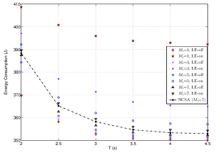
Figure 6: LEBS in bounding optimal solution for the 19-cell network.

From the two figures and Table IV, augmenting the size of local enumeration of interference (i.e., parameter $M_{i}$) leads to progressively tighter bounding intervals. Note that, even with $M_{i}$ being as small as one, that is, only a single neighboring BS is accounted for, the accuracy remains satisfactory – the relative difference of the upper and lower bounds of global optimum is less than $8\%$ and $12\%$, respectively, for the two networks. We observe that when $T$ increases, the lower bound from LE-off tends to improve in relation to AOCCS or NCSA, whereas the upper bound from LE-on does not. This is because LE-on over-estimates interference, and for large $T$ the error grows because optimal clusters tend to be small (cf. Theorem 5). For LE-off, increasing $T$ has the reverse effect.

Table IV: Average accuracy of the bounding interval from LEBS.

	Relative difference between $E^{*}_{\text{LE-on}}$ and $E^{*}_{\text{LE-off}}$,
	$(E^{*}_{\text{LE-on}}-E^{*}_{\text{LE-off}})/E^{*}_{\text{LE-off}}\times 100\%$
	7-cell Network	19-cell Network
$\bm{M_{i}=1}$	7.31%	11.87%
$\bm{M_{i}=3}$	3.21%	4.49%
$\bm{M_{i}=5}$	1.25%	1.92%
$\bm{M_{i}=7}$	0%	0.71%
$\bf Neighbor$-$\bm{M_{i}}$	0.58%	0.98%

NCSA combines LE-on with post-processing. From Figure 6, NCSA performs extremely close to global optimum for the 7-cell network – the relative deviation is merely 0.7% or less. For the 19-cell network, global optimum is not available for evaluating NCSA. However, the lower bound of global optimum, derived from LE-off, reveals that the deviation from global optimum is within 1%. This demonstrates the performance of NCSA as well as the usefulness of the bounding scheme. Moreover, from the last row of Table IV, setting $M_{i}$ based on the number of one-hop neighbors significantly outperforms uniformly setting $M_{i}=5$, while the problem sizes in LEBS are comparable for the two settings. The cell-adaptive choice of $M_{i}$ achieves similar performance as setting $M_{i}=7$. However, the problem size is considerably smaller in the former because $M_{i}<7$ for most cells.

VII Conclusions

We have considered optimal base station clustering and scheduling with the objective of minimizing energy consumption. Theoretical insights and mathematical formulations have been provided. For problem solution, we have presented a column generation approach, as well as a local enumeration scheme. The latter effectively addresses the difficulty of optimal cluster formation that is of combinatorial nature. Integrating column generation with local enumeration not only leads to flexibility in balancing optimality with scalability, but also yields lower and upper bounds confining the global optimum. Numerical results demonstrate that the algorithmic notions result in significant improvement in energy saving in comparison to existing schemes. In addition, the BS clustering and scheduling solutions that have been obtained are very close to global optimum.

The work in this paper provides a theoretical framework of optimizing BS clustering and activation. The proposed framework can be potentially implemented using the almost blank subframes (ABS) scheme defined in 3GPP Release 10. The BSs during their deactivation time durations can be set to the ABS mode, in which only control channels can be used with very low power, whereas the active BSs are in normal transmission mode. Also, from a scalability standpoint, the use of NCSA with local enumeration of interference has two implications. First, the problem size grows only linearly instead of exponentially in the number of BSs. Second, performance calculation for each BS needs to consider the neighboring BSs only. As such, the signaling cost for implementing the framework is reasonable.

An extension of the current work is to investigate the potential of power control. Base station clustering with cooperative multi-point transmission is another topic for future studies.

References

- [1] G. Fettweis and E. Zimmermann, “ICT energy consumption-trends and challenges,” in Proc. the 11th Int. Symp. on Wireless Personal Multimedia Commun., Sept. 2008, pp. 1–6.
- [2] K. Abdallah, I. Cerutti, and P. Castoldi, “Energy-efficient coordinated sleep of LTE cells,” in Proc. IEEE ICC, June 2012, pp. 5238–5242.
- [3] R. Litjens and L. Jorguseski, “Potential of energy-oriented network optimisation: Switching off over-capacity in off-peak hours,” in Proc. IEEE PIMRC, Sept. 2010, pp. 1660–1664.
- [4] M. Marsan, L. Chiaraviglio, D. Ciullo, and M. Meo, “Optimal energy savings in cellular access networks,” in Proc. IEEE ICC Workshops, June 2009, pp. 1–5.
- [5] S. Han, C. Yang, G. Wang, and M. Lei, “On the energy efficiency of base station sleeping with multicell cooperative transmission,” in Proc. IEEE PIMRC, Sept. 2011, pp. 1536–1540.
- [6] Z. Niu, Y. Wu, J. Gong, and Z. Yang, “Cell zooming for cost-efficient green cellular networks,” IEEE Commun. Mag., vol. 48, no. 11, pp. 74–79, Nov. 2010.
- [7] ETSI, “Evolved universal terrestrial radio access (E-UTRA) and evolved universal terrestrial radio access network (E-UTRAN); overall description; stage 2 (3GPP TS 36.300 version 10.5.0 Release 10),” ETSI TS 136 300 V10.5.0, Nov. 2011.
- [8] P. Frenger, P. Moberg, J. Malmodin, Y. Jading, and I. Gódor, “Reducing energy consumption in LTE with cell DTX,” in Proc. IEEE VTC Spring, May 2011, pp. 1–5.
- [9] K. Adachi, J. Joung, S. Sun, and P. H. Tan, “Adaptive coordinated napping (CoNap) for energy saving in wireless networks,” IEEE Trans. Wireless Commun., vol. 12, no. 11, pp. 5656–5667, Nov. 2013.
- [10] F. Han, Z. Safar, and K. Liu, “Energy-efficient base-station cooperative operation with guaranteed QoS,” IEEE Trans. Commun., vol. 61, no. 8, pp. 3505–3517, Aug. 2013.
- [11] S. Kompella, J. Wieselthier, A. Ephremides, H. Sherali, and G. D. Nguyen, “On optimal SINR-based scheduling in multihop wireless networks,” IEEE/ACM Trans. Netw., vol. 18, no. 6, pp. 1713–1724, Dec. 2010.
- [12] A. Capone, G. Carello, I. Filippini, S. Gualandi, and F. Malucelli, “Routing, scheduling and channel assignment in wireless mesh networks: Optimization models and algorithms,” Ad Hoc Netw., vol. 8, no. 6, pp. 545–563, Aug. 2010.
- [13] V. Angelakis, A. Ephremides, Q. He, and D. Yuan, “Minimum-time link scheduling for emptying wireless systems: Solution characterization and algorithmic framework,” IEEE Trans. Inf. Theory, vol. 60, no. 2, pp. 1083–1100, Feb. 2014.
- [14] A. Ouni, H. Rivano, and F. Valois, “A multi-objective optimization of broadband WMN: energy-capacity tradeoff and optimal System configuration,” INRIA, Report RR-7730, Sept. 2011. [Online]. Available: http://hal.inria.fr/hal-00619827
- [15] I. Siomina and D. Yuan, “Analysis of cell load coupling for LTE network planning and optimization,” IEEE Trans. Wireless Commun., vol. 11, no. 6, pp. 2287–2297, June 2012.
- [16] C. K. Ho, D. Yuan, and S. Sun, “Data offloading in load coupled networks: A utility maximization framework,” IEEE Trans. Wireless Commun., vol. 13, no. 4, pp. 1921–1931, Apr. 2014.
- [17] C. K. Ho, D. Yuan, L. Lei, and S. Sun, “Optimal energy minimization in load-coupled wireless networks: computation and properties,” in Proc. IEEE ICC, June 2014, pp. 2412–2417.
- [18] ——, “On power and load coupling in cellular networks for energy optimization,” IEEE Trans. Wireless Commun., 2014, available as pre-print.
- [19] K. Murty, Linear programming. Wiley, 1983.
- [20] P. Björklund, P. Värbrand, and D. Yuan, “Resource optimization of spatial TDMA in ad hoc radio networks: a column generation approach,” in Proc. IEEE INFOCOM, Apr. 2003, pp. 818–824.
- [21] C. Peng, S.-B. Lee, S. Lu, H. Luo, and H. Li, “Traffic-driven power saving in operational 3G cellular networks,” in Proc. ACM MOBICOM, Sept. 2011, pp. 121–132.
- [22] O. Arnold, F. Richter, G. Fettweis, and O. Blume, “Power consumption modeling of different base station types in heterogeneous cellular networks,” in Proc. IEEE Future Network and Mobile Summit, June 2010, pp. 1–8.
- [23] C. Lund and M. Yannakakis, “On the hardness of approximating minimization problems,” Journal of the ACM, pp. 960–981, 1994.
- [24] M. Lübecke and J. Desrosiers, “Selected topics in column generation,” Operations Research, vol. 53, pp. 1007–1023, 2004.