Critical dynamics of gene networks is a mechanism behind aging and Gompertz law

Abstract

Although accumulation of molecular damage is suggested to be an important molecular mechanism of aging, a quantitative link between the dynamics of damage accumulation and mortality of species has so far remained elusive. To address this question, we examine stability properties of a generic gene regulatory network (GRN) and demonstrate that many characteristics of aging and the associated population mortality rate emerge as inherent properties of the critical dynamics of gene regulation and metabolic levels. Based on the analysis of age-dependent changes in gene-expression and metabolic profiles in Drosophila melanogaster, we explicitly show that the underlying GRNs are nearly critical and inherently unstable. This instability manifests itself as aging in the form of distortion of gene expression and metabolic profiles with age, and causes the characteristic increase in mortality rate with age as described by a form of the Gompertz law. In addition, we explain late-life mortality deceleration observed at very late ages for large populations. We show that aging contains a stochastic component, related to accumulation of regulatory errors in transcription/translation/metabolic pathways due to imperfection of signaling cascades in the network and of responses to environmental factors. We also establish that there is a strong deterministic component, suggesting genetic control. Since mortality in humans, where it is characterized best, is strongly associated with the incidence of age-related diseases, our findings support the idea that aging is the driving force behind the development of chronic human diseases.

Introduction

Aging is a complex biological process. It occurs at every possible scale characterizing the living organism, ranging from the single cell level (e.g., oxidative damage, somatic mutations) to the level of interaction between different organs (e.g., failure of individual organs with age or accumulation of dangerous byproducts of metabolic activity such as arterial plaque). This is why it has been notoriously difficult to pinpoint the ultimate cause, a single molecular mechanism behind aging and relate it to such life-long consequences as the onset and progression of age-related diseases and, finally, death. As a consequence, a wide spectrum of propositions on the origin of aging has emerged over the years such as theories that view aging as a pre-programmed process Skulachev2001 ; Longo2005 , various concepts involving damage accumulation Partridge2002 ; Sinclair2009 ; Gladyshev2012 ; Gladyshev2013 ; ORGEL1973 , hyperfunction theory blagosklonny2006aging ; blagosklonny2009growth ; DeMagalhaes2012 , disposable soma theory Kirkwood1977 ; Kirkwood2000 , antagonistic pleiotropy williams2001pleiotropy and mutation accumulation theory medawar1952unsolved . Since the theories of aging often differ greatly from each other both in spirit and letter and reflect upon different “facets” of aging reis1989model ; Gladyshev2012 ; Gladyshev2013 ; gladyshev2016aging , it is not always possible to see their mutual inconsistencies and compatibilities.

One of the key ideas in the study of aging is the causal role of molecular damage. Over 40 years ago Leslie Orgel proposed an attractive damage-based theoryORGEL1973 , in which he argued that molecular corruption of enzymatic machinery of transcription and/or translation would produce positive feedback, leading to an “error avalanche”. We recently proposed a more general hypothesis of error accumulationkogan2014stability , supported by a semi-quantitative stability assessment for a generic gene regulatory network (GRN). We suggested a causal role of regulatory-error accumulation in the age-dependent increase in mortality rate, reflecting limited ability of cellular damage-response pathways to repair the consequences of internal or external stresses However, no underlying mechanism has been established thus far, for the interplay between the dynamics of error accumulation in transcription/translation/metabolic processes and the increase in mortality rates.

To identify such a link, here we develop a theory of GRN stochastic critical dynamics and show that under very generic assumptions GRNs of most species should be inherently unstable in order to be compatible with age-dependent behaviour of mortality rates. Applying the method of proper orthogonal decomposition Antoulas2009 to the publicly available age-dependent transcriptome and metabolome datasets of Drosophila melanogaster pletcher2002genome ; avanesov2014age , we demonstrate explicitly that autocorrelation functions of transcriptional and metabolic datasets for D. melanogaster exhibit stochastic exponential instability with a characteristic time scale, $t_{\alpha}$, which is of the same order as mortality rate doubling time $t_{{\rm MRDT}}$ of D. melanogaster. We provide explicit solutions for the stochastic aging dynamics of realistic GRNs to obtain expressions for the age-dependent mortality increase. We argue that the two time scales, $t_{\alpha}$ and $t_{{\rm MRDT}}$, should coincide for any species in which mortality follows the Gompertz equation. We are thus able to causally relate GRN instability to the characteristic Gompertzian increase of the mortality rate in populations. The exponential increase of mortality eventually slows down and the mortality rate is expected to approach a plateau, $M(t\gtrsim t_{{\rm ls}})\sim 1/t_{{\rm MRDT}}$, at late ages. The result should be valid for sufficiently long lived species, $t_{{\rm ls}}\gg t_{\alpha}$. The prediction is confirmed by quantative analysis of the transcriptomes, metabolomes and mortality curves for populations of D. melanogaster and mortality curves for very large cohorts of medflies vaupel1998biodemographic . We establish specific metabolites and genes as biomarkers of aging in D. melanogaster, examine the respective human orthologs, and provide their associations with genes and pathways commonly related to the major human chronic diseases.

We show that the dynamics of aging, as manifested in transcriptional and metabolic profiles, can be decomposed into both stochastic component, related to regulatory error accumulation in transcription/translation/metabolic pathways, and strong deterministic component, which can be naturally associated with a genetic program of an organism. We show that the presented model may serve to embrace most of the known features of the aging processes and hence provides a novel and universal basis for quantitative analysis of diverse age-dependent processes. We believe that the theoretical ideas presented in the paper could be useful in the identification of biomarkers and, after appropriate development, in mechanistic studies of processes that regulate aging in any sufficiently long-lived organism.

Results

Critical dynamics of Gene Regulatory Networks: quantitative model of aging

In this Section, we first explain the theoretical basis of our quantitative analysis of transcriptional and metabolic profile changes with age and construct a quantitative model of aging. We consider the case of the GRN described by a generic set of non-linear matrix equations of systems biology

$$g\left(x,dx/dt,d^{2}x/dt^{2},...\right)=F.$$

Here $g$ is a vector function of any number of quantities representing the state of the system, $x$, and its time derivatives which characterize the interactions between different components of $x$. If, for example, the state vector $x$ consists of the gene expression levels only, e.g. as in pletcher2002genome , the function $g$ may be thought of as encoding pathways to which the given genes contribute. In addition to gene expression levels, the state vector $x$ may include other descriptors, such as levels of metabolites avanesov2014age or methylation levels in DNA horvath2013dna . As the system state vector $x$ is not observable in its entirety, we presume that any sufficiently large part of it captures representative information about “macroscopic” properties of the biological system state at the organismal level. For the sake of simplicity, below we will refer to gene expression only, if not stated otherwise.

The vector $F$ describes the action of external or internal stress factors affecting components of $x$. The vector $F$ may depend on time, $t$: $F(t)=F_{0}+\delta F(t)$, where $F_{0}$ and $\delta F$ represent the mean stress and the fluctuations of stress levels, respectively.

Over long times, gene expression levels typically fluctuate near certain, relatively slowly changing, mean values, corresponding to the average homeostatic state of an organism. Therefore, we assume that there is always a quasi-stationary point $x_{0}$ (homeostasis of the organism), given by the solution of the stationary equation $f(x_{0})=F_{0}$. As a result, the slow dynamics of the fluctuations of the gene expression levels, $\delta x=x-x_{0}$, in its leading order obeys thе matrix stochastic equation for a linear continuum-limit of a Markov chain:

$$D\delta\dot{x}+K\delta x=\delta F,$$ (1)

where the matrices $D$ and $K$ describe the dynamical relaxation properties and the interactions between the components of the gene regulatory network, respectively (see Supplementary Information, Section A, for in-depth discussion of Eq.(1) derivation).

It has been previously suggested that, in most species, GRNs operate close to a stability-instability transition or order-disorder bifurcation balleza2008critical ; krotov2014morphogenesis ; kogan2014stability . The transition from stability to instability in networks with the network graphs not possessing specific symmetries is typically associated with occurrence of co-dimension $1$ bifurcations Fiedler2002 ; Seydel2009 . Such transitions are characterized by the loss of stability along a single direction in the state vector space, corresponding to the first principal component, while contributions from all other principal components remain stable. This situation, known in the literature as a saddle-node bifurcation Fiedler2002 , is realized when the smallest real eigenvalue, $\epsilon$, of the matrix $K$ tends to zero, $\epsilon\rightarrow 0,$ and then becomes negative. Accordingly, the stationary solution for $x_{0}$ ceases to exist, and the homeostatic state of the organism starts to change in time. As we shall argue, this very instability is directly responsible for the process of aging.

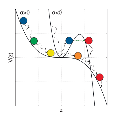
(A)

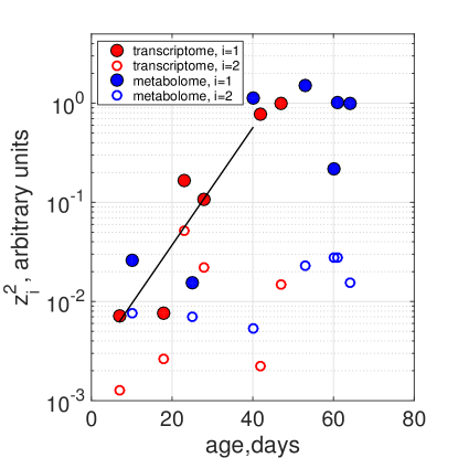
(B)

Figure 1: (A) Schematic representation of the stochastic dynamics in the effective potential $V(z)$ corresponding to the cases of unstable ($\alpha>0$) and stable ($\alpha<0$) GRNs, see Eq.(2). (B) Age dependence of $z_{1,2}=(\delta x^{T}\cdot b_{1,2})$ of the expressome state projections onto the vectors $b_{1,2}$ corresponding to the first two principle components as functions of age (gene expressions for normally fed D. melanogaster from pletcher2002genome , red, and metabolite levels for normally fed D. melanogaster from avanesov2014age , blue). Here $E(...)$ stands for the average over the biological repeats; $(a^{T}\cdot b)$ denotes a scalar product of two vectors $a$ and $b$.

(A)

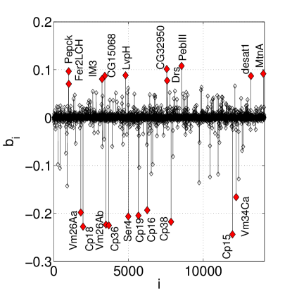
(B)

(C)

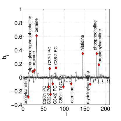
(D)

Figure 2: Basic biological evidence for the presented stochastic model of aging: (A) Mortality rate along with the projection $z$ of the system state vector, $\delta x$, represented by the transcriptomes of aging D. melanogaster pletcher2002genome , onto the singular direction $b$ of the covariance matrix $E(\delta x(t)\delta x^{T}(t^{\prime}))$ as a function of age. (B) Components of the vector $b$ for D. melanogaster. Peaks correspond to the values of the components of the vector $b$ for every gene in the dataset. (C) Mortality rate and the projection $z$ of the system state vector $\delta x$, represented by the metabolomes of D. melanogaster as a function of age avanesov2014age ; (D) Components of the vector $b$ for D. melanogaster, computed using only the levels of targeted metabolites avanesov2014age .

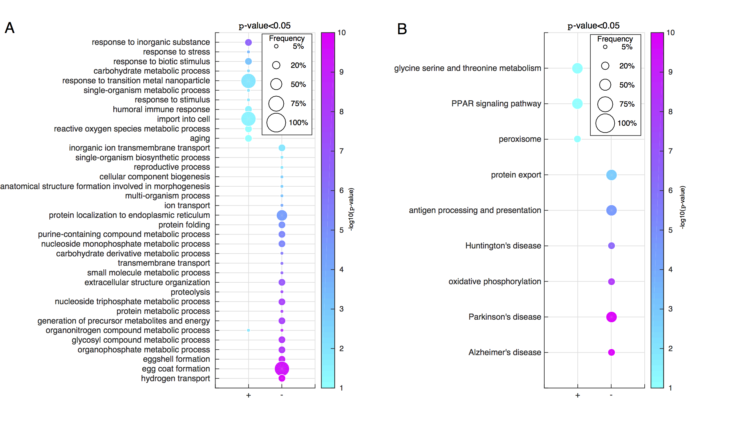
Figure 3: Biological characterization of the “leading direction of aging” $b$ in D. melanogaster: (A) Gene Ontologies (Biological Process only) enrichment by the leading positive and negative components of the vector $b$ computed using gene expression transcripts; (B) KEGG pathways enrichment for human orthologs of the gene sets representing the leading components of $b$, corresponding to positively and negatively regulated genes.

To be specific, hereinafter we focus on this scenario. As explained in Supplementary Information, Appendix A, the derivative $\delta x$ of any gene expression level becomes critical close to the co-dimension 1 bifurcation point. This implies that fluctuations of the expressome $\delta x$ are strongly amplified with age, the phenomenon known as critical slowing-down (see e.g. Suzuki2009 ). In particular, the autocorrelation time scale $t_{{\rm auto}}=(a^{T}\cdot Db)/\epsilon$ of the expressome diverges as $\epsilon\to 0$, indicating that stochastic dynamics of $\delta x$ is very slow near the point of bifurcation. The fluctuations of the expressome state vector $\delta x$ including those created in response to persistent external stress, are mostly amplified along the direction $b$ of the right eigenvector of matrix $K$ corresponding to the vanishing eigenvalue $\epsilon$. The latter observation is supported by the analysis of experiments in D. melanogaster, where transcriptional responses to different stress factors were found to contain a good fraction of similar differentially expressed genes in the limit of both nearly lethal brown2014diversity and weak stressors 10.1371/journal.pone.0086051 .

Accordingly, over times comparable to the average lifespan, the gene expression fluctuations are dominated by transcript-level changes along the vector corresponding to the leading principal component, which is collinear with the direction of the vector $b$. We conclude that for long time intervals evolution of the vector of the GRN state vector, $\delta x$, can be accurately described using a single variable $z$, such that $\delta x\approx z\cdot b$. Accordingly, Eq.(1) can be reduced to the equation

$$\frac{dz}{dt}+\frac{\partial V(z)}{\partial z}=f,$$ (2)

describing the Brownian motion of a particle in an effective potential $V(z)\approx-\alpha z^{2}/2$, for sufficiently small $z$, and the quantity $\alpha=-\epsilon/(a^{T}\cdot Db)$ characterizes the “stiffness” of the gene regulatory network. The stochastic force, $f=(a^{T}\cdot\delta F)/(a^{T}\cdot Db)$, is a single unified quantitative measure of stochastic component of all external and internal stress, and is characterized by the diffusion coefficient $\Delta$ (see Supplementary Information, Appendix A for the in-depth derivation and necessary justification).

Depending on the specific morphological properties of the gene regulatory network, the curvature of $V(z)$ at small $z$ can be negative, $\alpha<0$, or positive, $\alpha>0$, as shown in Figure 1A. The first case will be briefly considered in Discussion section. In the latter case, the GRN is inherently unstable, and the variance of gene expression levels, $C(t)$, computed using the solutions of Eq.(2), grows exponentially with age as

$$C(t)=E(\delta x(t)\delta x^{T}(t))\approx E(\delta x_{0}^{2})b\cdot b^{T}\exp(2\alpha t).$$ (3)

The expression (3) is fully consistent with earlier observation of increasing biological variability with age variability ; variabilityGerm .

Criticality of gene expression-level dynamics criticality implies that the parameter $\alpha$ is close to zero and hence the expressome covariance matrix $C(t)$ should be a matrix with special structure. Eq.(3) implies that in this case the right eigenvector of the covariance matrix corresponding to its largest eigenvalue coincide with the right eigenvector $b$ of the matrix $K$ corresponding to vanishing eigenvalue $\epsilon\rightarrow 0$ (see Supplementary Information, Appendix A). What is more, the largest eigenvalue should be much larger than all other eigenvalues of this matrix. In reality the properties of the experimental sample covariance matrix may be degraded by the experimental noise and necessarily very limited number of samples compared to the number of transcripts or metabolites observed.

These conclusions are supported by Principal Component Analysis (PCA) of the age-dependent shifts of RNA-transcript and metabolite levels in normally fed D. melanogaster from pletcher2002genome and avanesov2014age , respectively. The covariance matrices computed from such datasets are indeed almost singular, see Supplementary Information, Figure 4. Correspondingly, the variation of the state vector $\delta x$ with age is dominated by the change along the loading vector corresponding to the first principal component, and $z\equiv z_{1}$, where $z_{1}=(\delta x^{T}\cdot b)$ is the first principal component, as described in Figure 1B. The variance along this vector grows very quickly with age, both in the metabolome and the transcriptome, in accordance with Eq.(3). The exponent, roughly inferred from each of the datasets for ages less than the mean lifespan, appears to be nearly the same, which is an indication of the same GRN instability observed in each of the experiments. For the sake of comparison, we have also plotted projections of gene expression on the next principal component. It is easy to see that the transcriptome and metabolome remain dynamically stable along the direction of the second principal component.

We thus hypothesize that at the origin, $z\approx 0$, the expressome state corresponds to a healthy or “youthful” state, while larger values of $z$ phenotypically describe distorted states of aged animals. Accordingly, aging manifests itself as a slow dynamics of expression levels, an exponential roll-out along the singular, or “aging” direction $b$, from the younger animals to the older ones. The singular “direction of aging” $b$ is associated with a response to a generic stress and determined by the properties of the interactions in the network only. At least within the model assumptions, the direction $b$ does not depend on the detrimental stress factors and appears to be hard-coded in the genome, and hence the development along $b$ can be considered as an organism-level manifestation of an aging program or quasi-program khalyavkin2014aging ; arlia2014quasi ; blagosklonny2012answering ; blagosklonny2013mtor ). The “direction of aging”, vector $b$, is similar but not the same as the differential expression vector in aging animals, since the latter may include a contribution of faster modes represented by other eigenvectors of the GRN connectivity matrix $K$ corresponding to eigenvalues with larger absolute value. Since the network state fluctuations along all the other directions are not related to aging and are relatively small, we conclude that the deterministic component of aging in $\delta x(t)$ already dominates over the stochastic one, even early in life (also see below).

Gompertz mortality law and biological age

To relate the GRN instability to the process of aging we further assume that for every gene in the genome there exists a particular threshold associated with its over- or under-expression, which leads to a strong build-up of deleterious changes, which in it turn ultimately lead to death. Since fluctuation of the expression levels can be written in the form $\delta x\approx z\cdot b$, such deleterious thresholds can be defined by the specific values of $z=Z_{i}$ for every gene, which may be either positive or negative. It is reasonable to assume that the death of a cell (and ultimately of an organism) occurs once $z$ reaches the smallest (by absolute value) of the threshold values, $z=Z$. In Supplementary Information Section B we argue, that as the expressome state deviates from the initial point, the higher order non-linearities in Eq.(1) and therefore in the effective potential $V(z)$ of Eq.(2) can no longer be neglected. As expected from the argument, we are able to show in Supplementary Information section B, that the threshold value $Z$ can be equally well introduced formally in the model as the single effective property of the non-linearity in such a way that $Z$ is large whenever the non-linear interactions are weak..

Initially, the probability density along the aging direction is localized at a small value of $z$ and the mortality is also very small. If severe deleterious changes occur late in life, i.e. if $\gamma=\alpha Z^{2}/\Delta\gg 1$, the lifespan greatly exceeds $t_{\alpha}$, the non-linearity is small, and the mortality increases exponentially with age first, then the growth decelerates, and, eventually, the mortality reaches a plateau. At intermediate ages, in a narrow range close to the average lifespan of the animals, the mortality can be approximated with

$$M\approx\text{0.61$\alpha$}e^{\alpha(t-t_{{\rm ls}})}\sim\frac{\Delta}{Z^{2}}e^{\alpha t}.$$ (4)

This is a form of the Gompertz law gompertz1825nature (see Supplementary Information, Appendix B for the complete analytical solution for the age-dependent mortality in a closed form for all ages). The Gompertz exponent $\alpha$ is related to the Mortality Rate Doubling Time (MRDT), $t_{{\rm MRDT}}$, by equation $\alpha=\log(2)/t_{{\rm MRDT}}$. In practice, the value of $\alpha$ is often determined from the survival records at the age, corresponding to a narrow interval of width $\sim 1/\alpha$ around the mean lifespan, when most of the animals die. Therefore Eq.(4) suggests that the empirical Gompertz exponent should be very close to the GRN “stiffness”.

On the other hand, the Initial Mortality Rate (IMR), $\Lambda_{{\rm IMR}}$, is related both to the stress levels and to the time required to reach the boundary $Z$ under the action of the random damaging forces only, $\Lambda_{{\rm IMR}}=\Delta/Z^{2}$. Normally, the stochastic forces are weak, $\gamma\sim(\alpha/\Lambda_{{\rm IMR}})$ is large, and, therefore, average lifespan, $E(t_{{\rm ls}})\sim\alpha{}^{-1}\log\gamma\gg\alpha^{-1}$, is also large compared to the characteristic time, associated with the gene network instability, $t_{\alpha}\sim\alpha^{-1}$. Remarkably, the lifespan in the model depends on the morphological properties of the GRN, such as its topology and connectivity, through the matrix $K$, and, more specifically, through its lowest eigenvalue $\epsilon\sim\alpha$. The dependence of species lifespan on damaging factors through the parameter $\Delta$ is, on the contrary, logarithmically weak. This has been recently shown in analysis of data from katzenberger2013drosophila in our workkogan2014stability , where long-term effects of traumatic brain injury at young age led to significant, but small changes in organismal lifespan. This also means that the gene-network evolution along the aging direction is practically deterministic in sufficiently long-lived organisms. At the same time, the stochastic forces are still very important early in life, yielding a relatively wide distribution of transcription profiles even in a group of otherwise identical animals at birth. Our analysis proposes that the stochastic component of the GRN dynamics explains the distribution of the observed ages at death in such a cohort.

Mortality in a form similar to Eq.(4) can be associated with gene network instability in a simple phenomenological model, where both IMR and MRDT were expressed in terms of generic network parameters, such as translation, gene repair and protein turnover rates, along with the stress levels, whereas mortality is directly associated with the increasing number of regulatory errors kogan2014stability . Therefore, the quantitative indicator of the expressome remodeling along the aging direction, $z$, can be interpreted as a measure of damage accumulated over the lifespan of an organism.

As we show in Supplementary Information, Appendix B, the dynamics of gene expression levels $\delta x$ in the weak non-linearity, or “Gompertzian” ,limit, $\gamma\gg 1$, proceeds along a well-defined trajectory, corresponding to a continuation of the development program. The “distance traveled” along the aging direction up to current moment of time, $z\sim(\delta x^{T}\cdot b)$, is, according to Eq.(4), directly related to mortality and hence by itself is a good biomarker of mortality and aging. These observations pave the way to define biological “clocks” using any number of variables characterizing a GRN state. For example, Figures 2A & C suggest the possibility of developing transcriptome- and metabolome-derived biological clocks for D. melanogaster. Those clocks in turn may be compared with the biomarkers of aging and the biological age calculator (biological clock) similar to, for example, the one derived from a regression model established using age-dependent DNA-methylation patterns horvath2013dna .

Association between GRN instability and mortality rate

Our analysis of D. melanogaster age-dependent transcriptional data from pletcher2002genome indicates that the gene expression variance grows exponentially with age in agreement with Eq.(3), with $\alpha\approx 19.1\,{\rm yr}^{-1}$, as shown in Figure 2A. In a similar fashion we have studied the “direction of aging” $b$ in the metabolome of D. melanogaster avanesov2014age . The projection of the metabolome state vector onto the singular direction $b$ increases very quickly with age, along with the reported mortality as shown in Figure 2C. The mean lifespan of D. melanogaster is about 25 and $40$ days in both experiments, respectively, and in the two cases the initial exponential growth of the projection $z^{2}(t)$ ceases at $t\gtrsim t_{ls}$, as predicted by the theory. Figure 1B represents a side-by-side comparison of the variance computed from the gene expression and the metabolome datasets. The values of instability rates, $\alpha$, recovered from analysis of both experiments, are very similar and close to the value of the Gompertz exponent $\alpha=\ln 2/t_{{\rm MRDT}}=17.1\,{\rm yr}^{-1}$ corresponding to the mortality rate doubling time $t_{{\rm MRDT}}\approx 0.04\,{\rm yr}$ tacutu2013human .

The pace of mortality-rate increase slows at advanced ages

At more advanced ages, $t\gtrsim E(t_{{\rm ls}})$, where $t_{{\rm ls}}$ is the average lifespan of the population, solutions of Eq.(2) exhibit deceleration of mortality. More specifically, as shown in Supplementary Information, Appendix B, we expect that the mortality rate ceases growing and saturates at a constant value, $M_{\infty}\sim\alpha$. This quantitative prediction can be compared with the experimental data for medflies vaupel1998biodemographic , where the cohort sizes were sufficient to observe both the regime of exponentially increasing mortality and the mortality plateau (see Supplementary Information, Figure 7). For the male medflies we find the asymptotic value $M_{\infty}\approx 0.16\,{\rm day^{-1}}$, which is close to the Gompertz exponent $\alpha\approx 0.22\,{\rm day}^{-1}$, in accordance with theoretical prediction. The asymptotic value of the mortality rate for female medflies, $M_{\infty}\approx 0.12\,{\rm day}^{-1}$, is also of the right order of magnitude, though nearly two times smaller than the slope of the mortality exponent $\alpha=0.25\,{\rm day^{-1}}$. Nevertheless, there is an approximate agreement between between the asymptotic value $M_{\infty}$ of the mortality rate at late ages and the value of the Gompertz exponent $\alpha$ in both cases. We also note that the approximate Eq.(4) should work better for longer living, or “Gompertzian”, $\Lambda_{{\rm IMR}}\ll\alpha$, organisms.

Biomarkers of aging in D. melanogaster

We computed the aging direction based on the transcriptomic data from Drosophila melanogaster pletcher2002genome . Gene Ontolology (GO) analysis of the leading components of $b$ vector is summarized in Figure 3A, for Biological Process (BP) categories only. The genes providing the most significant negative contribution to the aging direction $b$ can be roughly split into three groups. First, there is a large group of genes related to metabolic processes: organophosphate metabolism, generation of precursor metabolites and energy, membrane and mitochondrial ion transport. A detailed review of the GO categories involved seems to indicate that most of the down-regulated processes are related to oxidative phosphorylation or respiration. Another large group of genes involves developmental processes, such as anatomical structure formation involved in morphogenesis and extracellular structure organization. Genes encoding eggshell and egg coat formation correspond to strongly negative components of the vector $b$, which points to the reproductive senescence in female flies. Finally, we observe decline in processes related to proteostasis, including protein folding, ER localization and proteolysis.

As expected, the cluster of genes corresponding to the strongest positive components of the vector $b$ includes genes associated with a generic stress response. Among other leading components there are genes corresponding to the innate immune response (which is also a stress response), in agreement with previous conclusions khan2013aging , and the components of oxidation-reduction and reactive oxygen species metabolic processes.

We found that several transcription factors (TF) appear to be strongly associated with aging. One of the top positively associated genes, $hairy$, is a transcriptional suppressor, and believed to be a metabolic switch, found up-regulated in the gene expression datasets characterizing oxygen-deprived flies. Conversely, mutations in $hairy$ significantly reduce hypoxia tolerance zhou2008mechanisms . The only negatively associated transcription factor, $eve$, is a transcription factor involved in multiple organ and system development.

Human orthologs for biomarkers of aging in D. melanogaster

To obtain a better insight into aging of D. melanogaster we annotated gene expression changes involved in aging in flies with human orthologs. This is possible to do since according to OrthoDB, approximately 80% of all genes in D. melanogaster have human orthologs. We searched for human orthologs of the leading contributors to the aging direction vector $b$ computed from the transcriptome of D. melanogaster. The results of this analysis are represented in Figure 3B. Remarkably we observe transcriptional changes associated with human age-related diseases: the downregulated genes were enriched in KEGG categories corresponding to age-related neurodegenerative diseases (Huntington’s, Parkinson’s and Alzheimer’s), and also the processes of cardiac muscle contraction. We also observed that the downregulated genes enriched in KEGG pathways were associated with oxidative phosphorylation (consistent with the GO annotation and KEGG enrichment results above). In contrast, KEGG PPAR signaling pathway is activated with age, which may be another indication of the activation of anti-oxidant metabolism systems as noted above. There is evidence suggesting that PPARα and the genes under its control play a role in the evolution of oxidative stress increases observed in the course of aging in mice poynter1998peroxisome .

Further evidence relating the stochastic instability of the gene regulatory network to the common age-related diseases is a strong positive contribution of the Pepck gene, which encodes a rate-controlling enzyme of gluconeogenesis, the process by which cells synthesize glucose from metabolic precursors. RNAi silencing of the Pepck gene was found to be an effective way to reverse diabetes-induced hyperglycemia in micegomez2006overcoming . It has also been shown that expression of the Pepck ortholog in Caenorhabditis elegans correlates almost perfectly with longevity in an isogenic series of longevity mutantstazearslan2009positive . Also, a transgenic mouse strain constitutively overexpressing muscle PEPCK is muscular and long-lived hanson2008born .

Discussion

Our analysis suggests that aging involves an organismal level manifestation of the inherent instability of gene regulatory networks. Proper orthogonal decomposition of age-dependent transcriptional and metabolite profiles shows that, for species which age in accordanсe with the Gompertz equation, the life-long dynamics of the transcriptional and metabolite profiles can be effectively described in terms of stochastic critical dynamics with a single degree of freedom; that dimension/component is identified by the projection of the expressome on the right eigenvector $b$ of the GRN connectivity matrix $K$, and associated with the eigenvalue $\epsilon$ which vanishes at the critical point. We establish that depending on the sign of $\epsilon,$ a GRN can be either stable or unstable. We further propose that changes in metabolite levels contribute to aging similarly to changes in GRN, e.g., through a buildup of certain metabolites and molecular damage beyond a certain level. We note that appearance of such deleterious thresholds is guaranteed, if non-linearities in the equation (1) for expressome levels are accounted for (see Supplementary Information, Appendix B). We show that in this limit mortality follows the form of the Gompertz law, i.e. it first increases exponentially with age and then saturates at a constant level, a prediction supported by experimental evidence. As predicted, we find approximate agreement between the rate of gene regulatory network instability and the value of mortality rate saturation. Thus we are able to demonstrate that Gompertzian aging is a property of organisms with inherently unstable gene regulatory networks, and thus the gene network instability is a process that directly contributes to aging, which can be observed in the form of an exponential increase of all-cause mortality with age.

Though stochasticity of the expressome is an essential part of the model, it should be noted that in the Gompertzian limit a wide variety of organisms exhibits similar dynamics of expression profiles. According to our theory, genetically programmed connectivity matrix $K$ can be represented by its low-rank approximation using its right eigenvector $b$ and the corresponding eigenvalue $\epsilon$. Such a direction can be interpreted as a genetically programmed mechanism of aging. It is important to note that this direction is identifiable from experimental data, thus allowing quantitative predictions to be made about a mechanism behind aging.

The stochastic model of aging presented here is fully compatible with, and in fact embraces, several prevailing theories and hypotheses of aging, in the following sense:

• programmed and quasi-programmed aging Skulachev2001 ; Longo2005 ; DeMagalhaes2012 . We have shown that aging-driven dynamics of the expressome $\delta x(t)$ can be separated into stochastic and deterministic components. The deterministic component of $\delta x(t)$ starts to dominate over the stochastic one even early in life, at roughly the same time as the low-rank approximation of the GRN connectivity matrix $K$ becomes prominent, as can be seen from the fact that the covariance matrix is singular and dominated by the aging direction. As the dynamics of the expressome $\delta x(t)$ is largely determined by the properties of the matrix $K$, we interpret the low rank approximation of $K$ as a program or a quasi-program of aging blagosklonny2006aging , though no statement about its evolutionary nature can be made. We speculate that the same direction that corresponds to aging occurs and is active during development, thus being consistent with quasi-programmed aging theory.

• hyperfunction theory blagosklonny2006aging ; blagosklonny2009growth . The single mode $\delta x=z\cdot b$, describing a large cluster of genes that make a dominant contribution to the process of aging, starts dominating the aging dynamics soon after the completion of development, and the stochastic effects on the expressome dynamics can be considered relatively weak blagosklonny2006aging ; blagosklonny2009growth . The expression of positive leaders of the aging direction $b$ will grow with time, which can be interpreted as hyperfunction. In the model proposed, death of the organism is associated with a threshold beyond which this organism dies, which can be interpreted in the manner of hyperfunction theory as excessive functions of gene products for positive leaders of aging direction. However, some significant differences from hyperfunction theory as proposed in blagosklonny2006aging ; blagosklonny2009growth should be noted. Namely, we do not have any experimental data to determine the role of aging direction in developmental processes so this connection remains speculative. Moreover, according to the theoretical model, changes along stable developmental directions will tend to diminish with time and will not contribute to changes in gene expression, so at least some fraction of genes involved in development will not contribute to aging.

• damage/error accumulation Partridge2002 ; Sinclair2009 ; Gladyshev2012 ; Gladyshev2013 . The stochastic component of the expressome $\delta x(t)$ can be interpreted as a result of accumulation of errors, e.g. regulatory errors. Though it becomes small compared to the deterministic component at late ages, its effects are strongly pronounced at all ages, as the mean square deviation $\sqrt{E(\delta x^{2}(t))}$ first grows with age at the same exponential Gompertz rate as the mortality $M(t)$ and later stabilizes at some constant level, contributing at late ages to the very process of organism passing beyond toxicity threshold and dying. Our analysis shows, that the stochastic forces shaping the expressome evolution early in life explain a wide distribution of the ages at death even in a genetically homogenous population. It should be noted that damage accumulation does not exclude the scenario of quasi-programmed aging, as damage is not limited to byproducts, errors and other molecular forms, but encompasses deleterious changes at all levels, or the deleteriome Gladyshev2012 ; Gladyshev2013 ; gladyshev2016aging .

The relationship just established between the critical dynamics of the gene regulatory network state vector and the Gompertzian mortality characteristic of most species allows one to consider the projection $z=(b^{T}\cdot\delta x)$ as a candidate biomarker of aging. Due to the low value of the eigenvalue $\epsilon$ the direction $b$ dominates the response to any generic stress. This, in fact, was already demonstrated in 10.1371/journal.pone.0086051 , where transcriptional signatures of responses to very different stresses were found to share a great number of gene expression changes.

The levels of gene expression or metabolites corresponding to the most significant components of the aging direction $b$ are strongly associated with age and age-related diseases. Therefore aging as described here, in terms of GRN instability, leads to the impairment of normal physiological functions, has characteristic biomarkers and phenotypes including signs of major diseases of aging, and produces exponentially increasing morbidity. Accordingly, the process of aging itself falls under the definition of a disease recently used by AMA for a common condition such as obesity american2013resolution . We must note here that therapeutic or experimental interventions aimed to counter-balance the age-related changes in gene or metabolite expression may not be very effective ways to extend lifespan of the species. For example, even though aging in D. melanogaster is associated with increased internal and external bacterial load, as well as with increased expression of antibacterial peptides, neither reducing the bacterial population with antibiotics nor reducing the humoral antibacterial response was able to extend lifespan ren2007increased . The transcription factor $hairy$ is overexpressed with age, and yet its inhibition does not result in lifespan increase zhou2008mechanisms . This reinforces the conclusion that the markers of aging are, in general, not the same as regulators of aging.

Even though most of the analysis in this manuscript is performed for D. melanogaster, our conclusions are generic and should be applicable to other species. Depending on the network and environmental parameters, realistic GRNs would not necessarily support a derivation of the Gompertz law. In fact, aging is extremely diverse across the tree of life jones2014diversity . We believe that one of the most intriguing form of a non-Gompertzian mortality law in the model may arise if the effective potential $V(z)$ has a local minimum with small but positive curvature, as in Figure 1A, $\alpha<0$. The higher order nonlinearities, such as the cubic terms in the effective potential, cannot be neglected anymore and in this case the genetic network turns out to be metastable. If the minimum of the potential $V(z)$ is separated from the region of large $z$ by a sufficiently high activation barrier (see Figure 1A and Supplementary Information, Appendix B), the mortality rate, determined by the probability of activation, is exponentially small and age-independent. This situation could be a physical picture behind the hypothesis that some animal species exhibit negligible senescence finch1994longevity This feature of our model may also explain the apparent lack of age-dependent changes in physiological parameters as well as mortality rates observed in the naked mole rat and some other species over long time periods buffenstein2005naked . This argument may also be supported by the analysis in kim2011genome ; loram2012age-related , where the number of the genes differentially expressed with age was compared between extremely long-lived species and mice and humans. These works show that the number of differentially expressed genes in species with negligible senescence is much lower than in mammals with Gompertzian aging.

Supplementary Information

Appendix A Stochastic dynamics of gene expression and metabolite levels

In the following, we explain the physical basis for Eq. (2) and provide its derivation. We also explicitly find the expressions for the mortality rate, the survival probability, the lifespan distribution function and the average lifespan of species with expressome subject to Eq. (2).

A.1 Getting a grasp on expressome dynamics. Model reduction and physical considerations

The analysis represented in this paper is mainly based on the observation that time series datasets describing changes of expressome profiles with age are often quite susceptible to Model Reduction techniques [18]. Proper orthogonal decomposition of dynamic (time-series) datasets for age-associated gene expression levels (and also metabolite levels or other “omics” datasets) [19, 52, 20] shows that the long-time behavior of any expressome $x$ is largely determined by a single component (see Fig. 4). The number of different principal components $PC_{n}$ representing the signal $x(t_{1}),\ldots,x(t_{m})$ cannot not exceed the number of time snapshot points in corresponding time series. Even though $m$ is typically limited and is very small compared to the number of transcripts or metabolites, , the clear dominance of a single component in the signal is a non-trivial fact. As we argue here, it carries important information about biological gene regulatory and metabolic networks; namely, it shows that such networks are pre-critical in a sense that will be explained below.

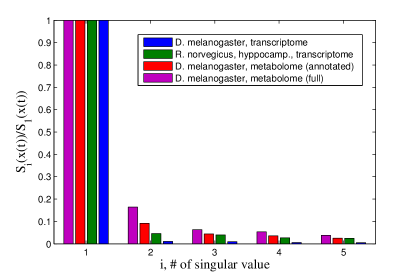
Figure 4: Five largest singular values $S_{i}(x(t))$ of the expressome $x(t)$ divided by the largest one, $S_{1}(t)$; transcriptome of D. melanogaster [19] (blue), transcriptome of R. norvegicus, hippocampus [52] (green), metabolome of D. melanogaster, targeted metabolites only [20] (red), metabolome of D. melanogaster, all metabolites [20] (purple). One of the orthogonal components of the expressome $x(t)$ clearly dominates over the others in all considered cases.

Consider a meta-stable gene regulatory network (GRN) with the instantaneous network state represented by a vector $x$, whose components $x_{i}$ are given by expression levels of different genes, proteins or metabolites participating in the GRN. Dynamics of the vector $x$ consists of mRNA levels, concentrations of proteins and metabolites, involved in regulatory pathways and are influenced by external as well as internal stress factors acting on the cell. This dynamics is governed by differential matrix equations of systems biology

$$g\left(x,\frac{dx}{dt},\frac{d^{2}x}{dt^{2}},\ldots\right)=F,$$ (5)

where $g$ is a vector function of the state vector $x$, encoding interactions between different components of the expressome, and the vector $F$ describes the action of (mostly stochastic) external or internal stress factors affecting components of $x$. For the sake of simplicity, below we will refer to gene expressions only, if not stated otherwise.

Generally speaking, the vector function $g$ may depend on arbitrarily high time derivatives $\frac{dx}{dt}$, $\frac{d^{2}x}{dt^{2}},\ldots,\frac{d^{n}x}{dt^{n}},\ldots$ of the expressome state vector. Hereinafter the focus of the study is on the dynamics of $x$ at time scales comparable to the mortality rate doubling time $t_{{\rm MRDT}}$, which is of the order of tens of days for nematodes and drosophilae and hundreds of days for mice. This time scale is to be compared to a typical time scale of protein translation and regulation, or a lifetime of mRNA. In order to describe this slow dynamics of the expressome state vector $x$, one can neglect all time derivatives of $x$ higher the first derivative $\frac{dx}{dt}$. The matrix Eq. (5) thus reduces to

$$g\left(x,\frac{dx}{dt}\right)=F.$$ (6)

A.2 Frequency domain properties of the vector $F$ of stress factors

As it was explained in the main text, the vector $F$ of environmental and internal stress factors affecting gene expression levels $x$ has both a slowly changing component, $F_{0}(t)$, and a stochastic component, $\delta F(t)$, rapidly changing in time. Below we assume for simplicity that $F_{0}(t)=F_{0}$, i.e., the slowly changing component is, in fact, constant.

Since dynamics of the vector $\delta F$ can be considered essentially random at time scales of interest, dynamics of $x$ is driven by correlation properties of $\delta F$. The total number of environmental and internal stress factors affecting gene expression levels $x$ is extremely large, and the vector $\delta F(t)$ represents a superposition of these factors. According to the central limit theorem [53] it can thus be considered a Gaussian stochastic process, so that

$$E(\delta F(t)\delta F(t^{\prime}))=B(t-t^{\prime}),$$

where $B(t-t^{\prime})$ is a function of the time difference $|t-t^{\prime}|$ only, while $E(\ldots)$ stands for the expected value of its argument. The statistical average is understood as average over ensemble of species/cells of a given organism. In the frequency domain, one has correspondingly

$$E(\delta F(f)\delta F(-f))=$$

$$=\int df\,e^{-2\pi if(t-t^{\prime})}E(\delta F(t)\delta F(t^{\prime}))=B(f),$$

where $f$ is frequency of a given mode in the Fourier expansion of the function $B(t-t^{\prime}).$

The function $B(f)$ has multiple singularities in the complex plane of $f$. These singularities encode characteristic time scales of pathways’ dynamics. However, the function $B(f)$ decays quickly with $f$ as $f\to\infty$. This guarantees that the amount of stress affecting the gene expression levels $x$ does not change very rapidly. On the other hand, the behavior of $B(f)$ is smooth at very small frequencies, i.e., $B(f)\to B$ as $f\to 0$, so that the amplitude of rare fluctuations of $\delta F$ remains limited. As we would like to understand the dynamics of $x$ at time scales comparable to $t_{{\rm MRDT}}$, we consider the case $B(f)\sim B$ in what follows. In this, the stochastic process $\delta F(t)$ in the right-hand side of Eq. (6) has correlation properties of white noise:

$$E(\delta F(t)\delta F(t^{\prime}))=B\delta(t-t^{\prime}),$$ (7)

where $\delta(t-t^{\prime})$ is the Dirac delta-function.

A.3 The vicinity of a stationary point (homeostasis)

When the fluctuations of the genotoxic forces are relatively weak, $|\delta F|\ll\left|F_{0}\right|$, the fluctuations of the expressome state vector are also small: $x=x_{0}+\delta x$, $\delta x\ll x_{0}$. Here $x_{0}$ is the stationary point given by the solution of the equation

$$g(x_{0})=F_{0}.$$

In the vicinity of this point Eq. (6) reduces to

$$D\delta\dot{x}+K\delta x+\Gamma^{(3)}\delta x\delta x+\ldots=\delta F,$$ (8)

where the matrices $D$ and $K$ describe the relaxation effects and the “interaction” between genes in the GRN. The matrix $\Gamma^{(3)}$ encodes the leading non-linear terms in the expansion of the vector function $g(x)$ in powers of small $\delta x$, with all other terms corresponding to the higher order non-linearities being omitted from the expansion. Generally, such non-linear terms are not small (in particular, they are not small at early times, close to the initial state of the expressome). However, a common feature of the dissipative network described by Eq. (8) is the decay of (most) components of $\delta x$ with time, which makes non-linearities in Eq. (8) less relevant at later stages of the time dynamics. Whether this feature holds for the GRN under consideration is a non-trivial question, which we shall now address.

A.4 Saddle-node bifurcation and critical slowing-down

Domination of a single principle component in the expressome vector $x(t)$ is not a generic prediction of the model (8). We would like to argue that such a dominance implies that GRNs under consideration are operating at the critical point. This critical point is a bifurcation, separating regimes of stable and unstable run-away behavior of the expressome $\delta x$.

Transition from stability to instability in networks with network graphs not possessing specific symmetries is typically associated with existence of co-dimension 1 bifurcations [25, 26]. Such transition is characterized by the loss of stability along a single orthogonal component of the network state vector. Contributions from all other orthogonal components remain stable. This situation is known in the literature as saddle-node bifurcation [25] and is realized when the lowest (real) eigenvalue of the matrix $K$ reaches zero and then becomes negative.

Let us denote the smallest (vanishing, but positive) eigenvalue of the matrix $K$ as $\epsilon$ and its corresponding left and right eigenvectors as $a$ and $b$. In order to understand dynamics of the expressome $\delta x$ near the GRN bifurcation, it is convenient to analyze the autocorrelation function $E(\delta x(t)\delta x(t^{\prime}))$. As shown in [54, 55], the latter is given by the following expression (in the frequency domain)

$$E(\delta x(t)\delta x^{T}(t^{\prime}))=$$

$$=\int df\cdot e^{-2\pi if(t-t^{\prime})}A^{-1}(f)E(\delta F(-f)\delta F^{T}(f))A^{*,-1}(f),$$ (9)

where $A(f)=i2\pi Df+K$. Its behavior is determined by the poles of the integrand in the complex plane of frequency $f$. In turn, the latter are given by the solution of the equation

$$\det(A(f))=0,$$

i.e., by the solution of the eigenvalue problem for the matrix $\pm i(2\pi)^{-1}D^{-1}K$. In particular, at very large time separations $|t-t^{\prime}|$ one finds that

$$E(\delta x(t)\delta x^{T}(t^{\prime}))\approx\frac{(a^{T}\cdot Ba)b\cdot b^{T}}{\epsilon(a^{T}\cdot Db)^{3}}\exp\left(-\frac{\epsilon|t-t^{\prime}|}{(a^{T}\cdot Db)}\right).$$ (10)

Several important observations can be made at this point: 1) as the parameter $\epsilon$ approaches $0$, amplitude of the autocorrelation function (10) grows as $\epsilon^{-1}$, i.e. fluctuations of the expressome vector are strongly amplified both with age and among the population (the statistical ensemble); 2) the autocorrelation time scale $\tau=(a^{T}\cdot Db)/\epsilon$ also grows strongly at $\epsilon\to 0$, implying that stochastic dynamics of the expressome becomes very slow near the point of bifurcation, a phenomenon known as critical slowing-down (see for example [27]); 3) fluctuations of the expressome vector $\delta x$ mostly develop along the direction $b$ of the right eigenvector of $K$ corresponding to the vanishing eigenvalue $\epsilon$, which in its turn guarantees that a single principal component of the expressome vector $\delta x$ dominates; 4) the corresponding left eigenvector $a$ determines directions of high sensitivity of the expressome to genotoxic stress factors $\delta F$. Other remaining eigenvalues of $-i(2\pi)^{-1}D^{-1}K$ have strictly positive real parts and thus correspond to contributions to (10), rapidly decaying with time. This guarantees that only one orthogonal component of $\delta x$ dominates, in accordance with experimental observations.

It should be noted that, when higher order derivatives in Eq. (5) are taken into account, this argument, albeit becoming more involved, remains valid: one has to construct the perturbation theory in powers of small parameter $\epsilon$, which still determines the smallest eigenvalue of the matrix $A(f)=K+i2\pi fD+(2\pi f)^{2}M+\ldots.$ Similarly to the case considered here, all higher eigenvalues of $A(f)$ possess positive real parts.

When $\epsilon$ crosses $0$ and becomes negative, the autocorrelation function (10) develops unstable behavior, again directed along the corresponding right eigenvector $b$ of $K$. In particular, one finds for the dispersion of the expressome at large $t$

$$E(\delta x(t)\delta x^{T}(t))\approx E(z^{2}(0))b\cdot b^{T}\exp\left(\frac{2\epsilon t}{(a^{T}\cdot Db)}\right),$$ (11)

where $E(z^{2}(0))$ is the dispersion of the projection $z=(\delta x^{T}\cdot b)$ of the expressome on the vector $b$, taken at the initial moment of time. The displacements of the expressome $\delta x$ along the other orthogonal components correspond to the dynamics of the gene network along the eigenvectors, characterizing the modes with finite and positive eigenvalues, and hence remain stable in time.

Thus, the quantity of interest in the critical regime $\epsilon\to 0$ is the projection of the expressome $\delta x$ on the right eigenvector $b$, $z=(\delta x^{T}\cdot b),$ which satisfies the Langevin equation

$$\frac{dz}{dt}=v\left(z\right)+\delta F^{\prime},$$ (12)

where $v\left(z\right)$ is the “velocity”, characterizing the motion along the $z$ coordinate. Next to the origin the velocity $v(z)\approx\alpha z$, where $\alpha=-\epsilon/(a^{T}\cdot Db)$. Here $\delta F^{\prime}=F/(a^{T}\cdot Db)$, is the stochastic force, such that $E(\delta F^{\prime}(t)\delta F^{\prime}(t^{\prime}))=\Delta\delta(t-t^{\prime})$, and $\Delta=(a^{T}\cdot Ba)/(a^{T}\cdot Db)^{3}$ is a property of the fluctuations. Since the vector $b$ is defined as eigenevector and subsequently is defined up to a factor, we can always select its direction in such a way as to make the collective coordinate $z$ increase with the age. It means that we can always limit our attention to the region $z>0$ only.

Appendix B Estimating mortality rates from the stochastic dynamics of an expressome

So far we have only considered stochastic dynamics of the expressome state vector $\delta x$ of an organism. To proceed with population properties, such as mortality, we need to construct a statistical description for populations, ensembles of organisms. Let us consider a large population of animals with the number of individuals $N(t=0)=N_{0}\gg 1$, born at the same moment of time, $t=0$. The development and aging of the animals in the population depends on the dynamics of the expression levels $x$ and can be naturally described in terms of the probability density $dN=N_{0}P\left(x,t\right)dx$, where $P(x,t)$ is the fraction of individuals within the population, characterized by the gene expression levels from the interval $(x,x+dx)$, and estimated at the time $t$. Another quantity of interest is the survival probability

$$S(t)=\int P\left(x,t\right)dx,$$

defined as the fraction of the animals, $N(t)/N_{0}$, surviving by the age $t$, relative to the initial size of the population $N_{0}$. The mortality rate can be found using the standard definition $M(t)=-(dS/dt)/S.$ In this Section we shall explain how to estimate the probability density $P(x,t)$, the survival probability $S(t)$, and the mortality rate $M(t)$ from the stochastic dynamics of the expressome state vector $\delta x.$

B.1 Estimating the probability density $P(z,t)$

B.1.1 Fokker-Planck equation

Following the arguments above we describe the process of aging as the slow changes in gene expression levels $\delta x$ over time governed by the Langevin equation (12). The probability $P(z,t)$ is the solution of the associated Fokker-Planck equation [56]

$$\frac{\partial P(z,t)}{\partial t}+\frac{\partial J\left(z,t\right)}{\partial z}=0,$$ (13)

where

$$J\left(z,t\right)=v(z)P(z,t)-\frac{1}{2}\Delta\frac{\partial P(z,t)}{\partial z}$$

is the probability flux along the direction $z$. We seek the distribution function $P(z,t)$ as the solution, corresponding to the initial condition $P(z,t=0)=P_{0}(z)$, and boundary conditions at $z=0$ and large $z$. To exclude the $z<0$ region we place a reflecting wall at $z=0$, which corresponds to

$$\left(\frac{\partial P(z,t)}{\partial z}\right)_{z=0}=0.$$ (14)

The suggested form of the boundary condition means that the $z>0$ and $z<0$ regions are totally isolated from each other.

We explore a Gaussian form of the initial condition in the form

$$P_{0}(z)=G\left(z\right)+G\left(-z\right),$$ (15)

$$G\left(z\right)=\frac{1}{\sqrt{2\pi}\sigma_{0}}e^{-\frac{(z-z_{0})^{2}}{2\sigma_{0}^{2}}},$$

characterized by the initial displacement $z_{0}$, and the distribution width, $\sigma_{0}$. The probability distribution (15) is an even functions and hence satisfies the boundary condition for (14) automatically. Therefore, the normalization condition takes the form

$$\intop_{0}^{\infty}dzP_{0}(z)=1.$$ (16)

In fact, in many practical situations Eq. (13) can be solved without the the boundary condition (14) using a simpler form of the initial distribution $P_{0}(z)=G\left(z\right)$. In this case the fraction of the animals

$$P_{-}=\frac{1}{2}\left[1-{\rm erf}\left(\frac{z_{0}}{\sqrt{2}\sigma_{1}}\right)\right],\quad\sigma_{1}=\sqrt{\sigma_{0}^{2}+\frac{\triangle}{2\alpha}},$$

will be, of course, lost to the unphysical region $z<0$. Therefore, the results of such a simplified calculation could only be trusted once the “leak” is sufficiently small, $P_{-}\ll 1$, or, equivalently, if $z_{0}\gg\sigma_{1}$. We distinguish between the two quantitatively different types of the initial conditions: the “deterministic”,

$$z_{0}\gg\sigma_{1},$$ (17)

and the “diffusive”, $z_{0}\ll\sigma_{1},$forms respectively.

For sufficiently small values of $z$ the “velocity” term in the Langevin equation (12) can be approximated by its linear expansion

$$v\left(z\right)=\alpha z.$$ (18)

For larger $z$ the nonlinearities set in and we employ a more general form

$$v\left(z\right)=\alpha z\phi\left(z\right),$$ (19)

where $\phi\left(0\right)=1$ is chosen to match the asymptotic expression (18) for small $z$. More specifically we expect that the function $\phi\left(z\right)$ increases at $z\rightarrow\infty$ fast enough, so that that $\ln(z)/\phi\left(z\right)\rightarrow 0$ (see the discussion below).

Biological states characterized by extremely large values of $z$ correspond to highly distorted expression profiles and therefore we assume, that the state $z=\infty$ is certainly associated with the death of the individual. Therefore, a physically relevant choice of the boundary condition at large $z$ is

$$P(z\to\infty,t)=0.$$ (20)

The Fokker-Planck equation (13) with the boundary condition in the form of Eq. (20) cannot be solved exactly. Fortunately, this is not really needed: a large amount of useful information about the stochastic dynamics of the expressome in relation to aging can be extracted from the asymptotic behavior of the probability density $P(z,t)$ in a few physically interesting regimes. The following analysis of the solutions of Eq. (13) is not, of course, new and we loosely follow the results presented in [57, 27] in the remaining of manuscript.

B.1.2 A toy model: absorbing wall at a large $z=Z$

Let us first collect a few well known results about the solutions of Eq. (13) for small $z$, where the drift velocity $v(z)$ can still be used in its linear form (18). If, for simplicity of the argument, the initial distribution is very narrow, $\sigma_{0}\rightarrow 0$ and $z_{0}=0$ ($G(z)\approx\delta(z)$), then the solution satisfying the boundary condition (20) is

$$P\left(z,t\right)=2G\left(z,0,t\right)=2\sqrt{\frac{\alpha}{\pi X\left(t\right)\varDelta}}\exp\left[-\frac{\alpha z^{2}}{X\left(t\right)\varDelta}\right],$$ (21)

where

$$G\left(z,z^{\prime},t\right)=\sqrt{\frac{\alpha}{\pi X\left(t\right)\varDelta}}\exp\left[-\frac{\alpha\left(z-z^{\prime}e^{\alpha t}\right)^{2}}{X\left(t\right)\varDelta}\right]$$

is the Green function of Eq. (13), and $X\left(t\right)=\exp\left(2\alpha t\right)-1$. Therefore, at sufficiently early times, $t\lesssim\alpha^{-1}$, the effect of the drift term is negligible and the behavior of $z$ is described by the diffusion equation with $v(z)\approx 0$. This means that at least in the beginning the solution is dominated by the effect of the random force $f(t)$ over the “deterministic” force $-\alpha z$ [57, 27].

Over time the deterministic force is taking over. It is instructive to observe the relevant regimes of the solution using a toy model first. To emulate the effect of the nonlinearity let us choose the form of the boundary condition at large $z$ in the form of a totally absorbing wall,

$$P(z=\pm Z,t)=0,$$ (22)

suggesting that the an organism dies whenever its $z$ reaches a certain threshold value $Z$. The solution (21) remains valid for sufficiently small ages,

$$t\lesssim\frac{1}{\alpha}\ln\left(Z\sqrt{\frac{\alpha}{\varDelta}}\right)\equiv t_{ls},$$ (23)

before the appreciable fraction of the animals reaches the $z\sim Z$, and hence $t=t_{ls}$ is of order of the lifespan in the population. Often the life expectancy $t_{ls}$ exceeds the GRN instability time scale, $t_{\alpha}\sim 1/\alpha$, or

$$\frac{\alpha Z^{2}}{\varDelta}\gtrsim 1.$$ (24)

It is shown below, that $\nicefrac{{\alpha Z^{2}}}{{\varDelta}}$ is the basic large parameter of our model. Whenever the ratio of the time scales is sufficiently large, the effects of the non-linearities are “weak” and a complete analytical treatment of the problem becomes possible and yields a series of universal results.

Technically, to meet the boundary condition (22) requirement, we add a loss term at the position of the absorbing wall,$-\eta\left(t\right)\left[\delta\left(z-Z\right)+\delta\left(z+Z\right)\right]$, where $\eta\left(t\right)$ is the Lagrange multiplier, an auxiliary function introduced to enforce the constraint (22). The analysis of the modified equation is straightforward and yields

$$P\left(z,t\right)=\varPhi\left(z,t\right)-$$

$$-\intop_{0}^{t}\left[G\left(z,Z,t-t^{\prime}\right)+G\left(z,-Z,t-t^{\prime}\right)\right]\eta\left(t^{\prime}\right)dt^{\prime},$$ (25)

where

$$\varPhi\left(z,t\right)=\intop_{-\infty}^{+\infty}G\left(z,z^{\prime},t\right)P_{0}\left(z^{\prime}\right)dz^{\prime}.$$

If the non-linearity is weak or the wall is far from current state of the system, i.e. whenever (24) holds, then $G\left(Z,-Z,t-t^{\prime}\right)\ll G\left(Z,Z,t-t^{\prime}\right)$, the function $\eta\left(t^{\prime}\right)$ varies very slowly with age compared to $G\left(Z,Z,t-t^{\prime}\right)$, and therefore

$$\eta\left(t\right)\approx\alpha Z\varPhi\left(Z,t\right).$$ (26)

For the case of Gaussian initial distribution (15) we have

$$\varPhi(z,t)=\frac{1}{\sqrt{2\pi}\sigma\left(t\right)}\left[e^{-\frac{(z-z\left(t\right))^{2}}{2\sigma^{2}\left(t\right)}}+e^{-\frac{(z+z\left(t\right))^{2}}{2\sigma^{2}\left(t\right)}}\right],$$ (27)

where $z\left(t\right)=z_{0}\exp(\alpha t)$, and the effective distribution width increases exponentially with age

$$\sigma^{2}\left(t\right)=\sigma_{0}^{2}+\sigma^{2}X\left(t\right),$$ (28)

where the combined quantity

$$\sigma=\sqrt{\sigma_{0}^{2}+\frac{\Delta}{\alpha}}$$

results from the initial probability density width broadening by diffusion at small $t$.

B.1.3 Weak non-linearity limit, general case

Let us turn our attention back to the general form of the non-linear drift velocity (19).At sufficiently small $z$ function $v(z)$ can be approximated by its linear expansion $v(z)\approx\alpha z$ and therefore Eq. (13) can be studied in its simplified form

$$\frac{\partial P(z,t)}{\partial t}+\frac{\partial}{\partial z}\left[\alpha zP(z,t)-\frac{1}{2}\Delta\frac{\partial P(z,t)}{\partial z}\right]=0.$$ (29)

We introduce a characteristic length scale $z\sim Z$, where the linear approximation to $v(z)$ fails. The age when $z\sim Z$ will correspond roughly to the lifespan of the organism, since, according to our assumptions, $v(z)$ grows fast enough at large $z$ and the point $z=\infty$ is reached in a finite time.

This linearized equation can be solved exactly with initial distribution (15) and boundary condition (20):

$$P(z,t)=\frac{1}{\sqrt{2\pi}\sigma}\exp\left\{-\alpha t-\frac{\left(ze^{-\alpha t}-z_{0}\right)^{2}}{2\sigma^{2}}\right\}$$ (30)

which would be a rightful approximation for solution of Eq. (13) in time region $t\ll t_{ls}$.

In the same time, at $t\gg\alpha^{-1}$ , irrespectively of the specific form of the nonlinearity, one can neglect the diffusion and set $\varDelta=0$. This means that the dynamics of the expressome is dominated by the drift term and is, therefore, deterministic. Accordingly, Eq. (13) can be transformed into

$$\frac{\partial P(z,t)}{\partial t}+\frac{\partial}{\partial z}\left[v\left(z\right)P(z,t)\right]=0.$$ (31)

One of the consequences of Eq.(31) is the fact that if a specimen is observed with an expressome state, corresponding to $z\gg\sqrt{\varDelta/\alpha}$, then the remaining life expectancy, or the time-to-death, for the animal is

$$\tau\left(z\right)=\intop_{z}^{\infty}\frac{dz^{\prime}}{v\left(z^{\prime}\right)},$$ (32)

and is finite. The integral on the r.h.s. is logarithmically divergent for the chosen type of non-linearity 19, which means that

$$\tau(z)=\frac{1}{\alpha}\ln\left(\frac{1}{z}\right)+\widetilde{\tau}\left(z\right),$$

and

$$\underset{z\rightarrow 0}{\lim}\widetilde{\tau}\left(z\right)={\rm const}$$

is finite.

The solution of Eq.(31) takes form $P(z,t)=P(z,\xi)=C(\xi)/\nu(z),$ where $\xi=t+\tau(z)$ and $C(\xi)$ is a function dependent on initial distribution and boundary conditions. One way to find it is to match the solutions of Eqs. (29) and (31) at some intermediate age $t_{1}$, lying in time region, where both equations can be used. Indeed, since normally $\alpha^{-1}\ll t_{ls}$ , we can use any $t_{1}$ such that

$$\alpha^{-1}\ll t_{1}\ll t_{ls}$$ (33)

as the matching point. The age range corresponds to $\sqrt{\Delta/\alpha}\lesssim z_{1}\lesssim Z$ interval. As the result, we obtain a closed form solution, applicable for deterministic initial condition (17) and boundary condition (20) for all ages $t\gtrsim 1/\alpha$

$$P(z,t)=\frac{\alpha k\left(z\right)}{\sqrt{2\pi}\sigma v\left(z\right)}\exp\left\{-\alpha t-\frac{\left[k\left(z\right)e^{-\alpha t}-z_{0}\right]^{2}}{2\sigma^{2}}\right\}.$$ (34)

Here

$$\widetilde{Z}=\underset{z\rightarrow 0}{\lim}e^{\alpha\widetilde{\tau}\left(z\right)}\sim Z,$$ (35)

and

$$k\left(z\right)=\widetilde{Z}\exp\left[-\alpha\tau\left(z\right)\right]$$ (36)

is auxiliary function with known asymptotic forms for the advanced ($\tau\left(z\right)\rightarrow 0$)

$$k\left(z\right)\rightarrow\widetilde{Z}\quad at\;z\rightarrow\infty,$$ (37)

and the early ($\tau\left(z\right)\rightarrow\infty$)

$$k\left(z\right)\rightarrow 0\quad at\;z\rightarrow 0$$ (38)

ages.

Let us turn to a more specific case of an arbitrary polynomial non-linearity

$$\phi\left(z\right)=1+\left(\frac{z}{Z}\right)^{\beta}$$ (39)

with $\beta>0$. The length scale here characterizes the non-linearity strength and hence large values of $Z$ correspond to the weak non-linearity limit (18). In accordance with the earlier definitions, it can be shown that $\tilde{Z}$ equals $Z$, and the remaining lifespan is

$$\tau\left(z\right)=\frac{1}{\alpha}\ln\left\{\frac{\left[Z^{\beta}+z^{\beta}\right]^{1/\beta}}{z}\right\},$$

and the probability distribution function takes the form of Eq. (34) with with $k\left(z\right)=z/\left[1+(z/Z)^{\beta}\right]^{1/\beta}$.

The absorbing wall at $z=Z$ situation, considered in the previous section, formally corresponds to $\beta=\infty$. Interestingly, the solution is still valid, $k(z)=z$ everywhere, if not immediately close to the wall, i.e. Eq. (34) matches the exact expression (25) for all $z\lesssim Z$. Hence we can conclude that the derived form of the probability density is universal, holds for an arbitrary form of the non-linearity, allowing for a finite lifespan. A specific form of the non-linearity is not important, all the information about the non-linear terms can be compressed into the length scale $Z$, being the single important parameter defining the lifespan and the form of the distribution function in the population.

Let us finish the section by computing the fraction of the animals, surviving by the age $t$. According to the definition,

$$S\left(t\right)=\intop_{0}^{+\infty}dzP\left(z,t\right)=$$

$$=\frac{1}{\sqrt{2\pi}\sigma}\intop_{0}^{Z}dk\exp\left\{-\alpha t-\frac{\left[k\left(z\right)e^{-\alpha t}-z_{0}\right]^{2}}{2\sigma^{2}}\right\}=$$

$$=\frac{1}{\sqrt{\pi}}\intop_{y_{1}}^{y_{2}}dye^{-y^{2}},$$

where, for $\alpha t\gg 1$,

$$y_{2}=\frac{Ze^{-\alpha t}-z_{0}}{\sqrt{2}\sigma},\;y_{1}=\frac{-z_{0}}{\sqrt{2}\sigma}.$$

That would lead us to expression

$$S\left(t\right)=\frac{1}{2}\left\{{\rm erf}\left[\frac{z_{0}}{\sqrt{2}\sigma}\right]+{\rm erf}\left[\frac{Ze^{-\alpha t}-z_{0}}{\sqrt{2}\sigma}\right]\right\}.$$ (40)

We also note, that

$$\intop_{0}^{+\infty}dzP\left(z,t\right)<1,$$

since the animals die and hence disappear at the infinity.

B.2 Estimating the first passage time, the survival probabilities, and the average lifespan

In the case under consideration, a more interesting quantity to calculate and analyze is not the probability density $P(z,t)$ itself, but a so-called first passage time distribution function $P_{{\rm FPT}}(t)$ [58, 59]. The reason is that the probability density $P(z,t)$ represents a sum over all possible stochastic trajectories $z(t)$, including those which pass the effective threshold $z=Z$ and then return back. On the other hand, by definition, $P_{{\rm FPT}}(T)$ is a probability for a given stochastic trajectory $z=z(t)$ to pass the threshold $z=Z$ at $t=T$ for the very first time. As such, it does not take into account trajectories which then re-enter the allowed domain of $z$.

When the “deterministic” form of the initial condition is chosen, the first passage time distribution function is given by

$$P_{{\rm FPT}}(t)=-\dot{S}\left(t\right)=$$

$$=\sqrt{\frac{\alpha}{\pi\varDelta}}\frac{2\alpha Ze^{2\alpha t}}{\left[X\left(t\right)\right]^{3/2}}\exp\left[-\frac{\alpha Z^{2}}{X\left(t\right)\varDelta}\right].$$ (41)

The function (41) grows exponentially at small $t\lesssim\alpha^{-1}$, possesses a distinct maximum at $t_{{\rm max}}=t_{ls}=\alpha^{-1}\ln\left[\left(\frac{\alpha Z^{2}}{\Delta}\right)^{1/2}\right]$, with its width $\delta t\sim\alpha^{-1}$ near the maximum and finally decays as $e^{-\alpha t}$ at $t\gg t_{{\rm max}},$ see Fig. 5. Computing the first passage time distribution function also allows one to easily estimate the survival probability $S(t)$, using the prescription $P_{FPT}(t)=-dS(t)/dt$. From Eq. (41) we find

$$S(t)={\rm erf}\left[\sqrt{\frac{\alpha Z^{2}}{2\Delta X(t)}}\right],$$ (42)

In the regime $\alpha^{-1}<t\lesssim t_{ls}$ , also known as Suzuki scaling [57, 27],equation for $P_{{\rm FPT}}(t)$ reduces to

$$P_{{\rm FPT}}(t)\approx 2\alpha Z\left(\frac{\alpha}{2\pi\Delta}\right)^{1/2}\exp\left(-\alpha t-\frac{\alpha Z^{2}}{2\Delta}e^{-2\alpha t}\right).$$ (43)

If the non-linearity is small, the center of the originally narrow distribution in the $z$-space follows the well defined trajectory $\bar{z}\left(t\right)=z_{0}\exp\left(\alpha t\right)$. At $t=t_{0}=\alpha^{-1}\ln\left(Z/z_{0}\right)$ it achieves the absorbing wall, which means that the average lifespan in the population described by the distribution is also $t_{ls}\approx t_{0}$. This result follows immediately from (40) and the exact definition of the average lifespan

$$t_{ls}=\intop_{0}^{\infty}dtS\left(t\right).$$ (44)

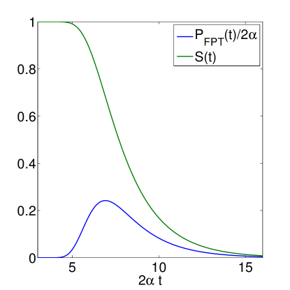
Figure 5: The first passage time distribution function $P_{{\rm FPT}}(t)$ (in units of $2\alpha$) and the survival probability $S(t)$ as a function of time $2\alpha t$; $\frac{\alpha Z^{2}}{\Delta}=1000.$

From Eq. (43) we find

$$S(t)\approx{\rm erf}\left[\left(\frac{\alpha Z^{2}}{2\Delta}\right)^{1/2}e^{-\alpha t}\right],$$ (45)

expression precise up to terms, exponentially small at $\frac{\alpha Z^{2}}{\Delta}\gg 1$, i.e., when a species is considered long-lived compared to the characteristic time scales of molecular dynamics in the cell, see the next Subsection. The function (45), initially exponentially close to $1$, then falls off quickly (as we shall see below, this fall-off corresponds to an exponentially growing mortality rate) and finally approaches zero as $\exp(-\alpha t)$ at $t\gg t_{ls}$.

B.3 Behavior of the mortality rate

As usual, the mortality rate is defined as $M(t)=-S^{-1}\cdot dS/dt$, so that one has precisely

$$M(t)=\frac{P_{{\rm FPT}}(t)}{S(t)}.$$ (46)

Once again, for the very narrow initial distribution (20), $\sigma_{0}\rightarrow 0$ and $z_{0}=0$ ($G(z)\approx\delta(z)$), we find, that

$$M\left(t\right)=\sqrt{\frac{\alpha}{\pi\varDelta}}\frac{2\alpha Ze^{2\alpha t}}{\left[X\left(t\right)\right]^{3/2}}\exp\left[-\frac{\alpha Z^{2}}{X\left(t\right)\varDelta}\right]\times$$

$$\times\left\{{\rm erf}\left[\sqrt{\frac{\alpha Z^{2}}{2X(t)\Delta}}\right]\right\}.^{-1}$$ (47)

For a more realistic determenistic form of the probability distribution at the origin 17 the solution is still possible, and for sufficiently advanced ages, $t\gg\alpha^{-1}$, we obtain

$$M\left(t\right)=\frac{Z\alpha}{\sigma}\sqrt{\frac{2}{\pi}}\exp\left[-\frac{\left(Ze^{-\alpha t}-z_{0}\right)^{2}}{2\sigma^{2}}-\alpha t\right]\times$$

$$\times\left\{1+{\rm erf}\left[\frac{Ze^{-\alpha t}-z_{0}}{\sqrt{2}\sigma}\right]\right\}^{-1},$$ (48)

once the non-linearity is sufficiently weak, as commanded by the condition (24).

B.3.1 Vanishing mortality at very early ages $t\ll\alpha^{-1}$

At sufficiently early ages $t\ll\alpha^{-1}$ behavior of $z$ is dominated by the effect of the random force $f(t)$ over the “deterministic” force $v(z)$ [57, 27]. Accordingly, the state variable and its fluctuations grow exponentially with age. This conclusion is confirmed by the analysis of senescence-associated transcriptional dynamics. It is worth emphasizing that the characteristic time scale of the stochastic growth of the expressome is $\sim\alpha^{-1}$. It thus depends only on the morphological properties of the GRN and does not depend on the genotoxic stress amplitude $\Delta$ at all.

At very early ages $t\ll\alpha^{-1}$ the first passage time distribution function is exponentially strongly suppressed:

$$P_{{\rm FPT}}(t)\approx\frac{2\alpha Z}{(2\alpha t)^{3/2}}\left(\frac{\alpha}{2\pi\Delta}\right)^{1/2}\exp\left(-\frac{Z^{2}}{4\Delta t}\right).$$ (49)

In this regime the survival probability $S(t)$ remains exponentially close to $1$:

$$S(t)\approx 1-\frac{2}{\sqrt{\pi}}\left(\frac{4\Delta t}{Z^{2}}\right)^{2}\exp\left(-\frac{Z^{2}}{4\Delta t}\right).$$

Therefore, the mortality rate remains exponentially close to $0$, and one approximately has $M(t)\approx P_{{\rm FPT}}(t)$. In our opinion, this behavior might explain relatively small mortality, often observed in cohorts at very early ages. We note that the behavior of the mortality rate in this regime is not universal as it strongly depends on the amplitude $\Delta$ of stochastic genotoxic stress.

B.3.2 Gompertz behavior at later ages $t\sim\alpha^{-1}$

As was explained above, as the age increases, the effect of the stochastic force $\delta F$ in Eq. (8) quickly becomes negligible in comparison to the effect of the “deterministic” force $-K\delta x$; the stochastic regime is changed by the drift motion at $t\sim\alpha^{-1}$. Correspondingly, the behavior (49) quickly changes when $t\gtrsim\alpha^{-1}$, yielding a Gompertz-like dependence of the mortality rate on age: $M\left(t\right)\approx M_{0}\exp\left(\gamma t\right)$, where the exponent

$$\gamma\left(t\right)=\frac{d}{dt}\ln M\left(t\right)\sim\frac{\alpha Z^{2}\dot{X}\left(t\right)}{X^{2}\left(t\right)\varDelta}\sim\alpha\frac{\alpha Z^{2}}{\varDelta}\gg\alpha$$

is found from Eq. (47) and is much greater than the GNR instability parameter $\alpha$.

B.3.3 Universal Gompertz behavior in the regime of Suzuki scaling

At even later times of the order $t\sim t_{ls}$, when the regime of Suzuki scaling is realized, we also find a universal Gompertz behavior. As was explained above, the first passage time probability distribution $P_{{\rm FPT}}$ reaches a maximum at $t_{{\rm max}}=\alpha^{-1}\ln\Lambda=t_{ls}$, where $\Lambda=\frac{\alpha^{1/2}Z}{\Delta^{1/2}}$, and its half-width near the the maximum is of the order $\alpha^{-1}$, as in Fig. 5. By the time $t\sim t_{{\rm max}}$ the argument of the error function in Eq. (45) is already sufficiently small for it to be expanded. One thus has

$$S(t)\approx\frac{2}{\sqrt{\pi}}\Lambda e^{-\alpha t}-\frac{2}{3\sqrt{\pi}}\Lambda^{3}\exp(-3\alpha t)+\ldots.$$

On the other hand, one finds for $P_{{\rm FPT}}(t)$ in the same regime

$$P_{{\rm FPT}}(t)=\frac{2\alpha\Lambda}{\sqrt{\pi}}e^{-\Lambda^{2}\exp(-2\alpha t)}e^{-\alpha t},$$

so that approximately

$$M(t)\approx\alpha e^{-\Lambda^{2}\exp(-2\alpha t)}.$$

Introducing $t=t_{{\rm max}}+\delta t$ one finally finds at small $\delta t\lesssim(2\alpha)^{-1}$

$$M(t)\approx e^{-1/2}\alpha e^{\alpha\delta t}\approx 0.61\alpha e^{\alpha\delta t}.$$ (50)

Thus, the Gompertz law with the universal exponent $\alpha^{-1}$ is realized at times $t_{{\rm max}}-(2\alpha)^{-1}\lesssim t\lesssim t_{{\rm max}}+(2\alpha)^{-1}$. We again emphasize that the Gompertz aging rate $\alpha$ depends only on the properties of the GRN under consideration and does not depend on stress. In fact, the very same conclusion holds for the Gaussian initial distribution case (48).

B.3.4 Mortality deceleration at late ages

Finally, at $t\gg t_{{\rm max}}$ both the first passage time distribution function (41) and the survival probability (42) decay exponentially. This corresponds to an asymptotically constant behavior of the mortality rate in both cases, (47) and (48):

$$M(t)\approx\alpha,$$ (51)

see Fig. 6. For late $t$, corrections to the leading constant term become exponentially small with time. The existence of mortality plateau in models of the type (8) is known in literature [60, 61].

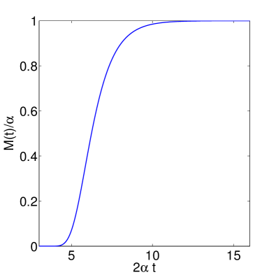
Figure 6: The mortality rate $M(t)$ for the case of the “diffusive” initial condition; $\alpha Z^{2}/\varDelta=1000.$ The maximum of $P_{{\rm FPT}}(t)$ is reached at $2\alpha t\approx 6.9$.

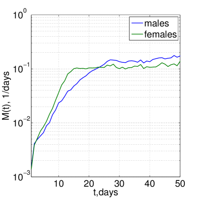
Figure 7: The mortality rate as a function of age from the very large cohorts study, medflies, males and females from [21].

B.4 Concluding remarks on aging regimes phenomenology

B.4.1 The unstable case, Gompertz limit, $\alpha Z^{2}/\varDelta\gg 1$

This case includes situations with a very weak non-linearity in the Fokker-Planck equation (13) and corresponds to a very high toxicity threshold $Z$ as compared to the characteristic amplitude of fluctuations of the stress factors $\Delta.$ As was explained above, we expect a species with such a GRN to be relatively long-lived, as the average life expectancy (23) is logarithmically larger than the inverse Gompertz exponent $\alpha^{-1}$. Four very distinct regimes of mortality exist for such species: (a) the regime of small mortality at early ages, (b) a Gompertz regime with the Gompertz exponent $\sim\alpha^{2}Z^{2}/\varDelta\gg\alpha$, (c) a Gompertz regime with a universal Gompertz exponent $\alpha$ and finally (d) a regime of constant mortality $M_{\infty}=\alpha$. On the other hand, if indeed $Z\gg\sigma_{0}$, the initial Gompertz exponent in regime (b) is very large, and a population of moderate size simply dies out before the regime of mortality slowing-down is observed.

B.4.2 The unstable case, short lifespan limit, $\alpha Z^{2}/\varDelta\gtrsim 1$

There are again four distinct regimes (a-d) of aging discussed above, with that difference that the regime (b) is hard to observe or unobservable, so a Gompertz regime (c) with the exponent $\sim\alpha$ is observed. Clearly, the regimes (c) and (d) are closely connected to each other in the sense, described above, and there is a strong correlation between the observed value of the Gompertz exponent and the mortality rate $M_{\infty}$ at late ages. This, as it seems, is what we observe e.g. in experiments with extremely large cohorts study of medflies, males and females from [21], see Fig. 7. A relatively short average lifespan of such species is comparable to the value of Gompertz exponent.

B.4.3 The stable case, $\alpha<0$

In this case, arguably the most interesting to consider, the effective potential $V(z)$ of the Langevin equation possesses a local minimum, separated from the roll-down to $z\to\infty$ by a potential barrier, see Fig. 1B of the main text. There exists a single regime of aging realized for the GRN of this type. It is characterized by a constant mortality rate $M_{\infty}$, its value being determined by the exponentially small Kramers probability of passage through the barrier[62]. If a GRN with such properties indeed exists in nature, it would correspond to a species with negligible senescence. We leave the in-depth study of this regime for a future work.

Appendix C Gene annotation

To analyze the vector $b$, obtained from the transcriptome of D. melanogaster [19], we have performed a gene set enrichment analysis for the components of vector $b$ using “Parent-Child-Intersection” GO enrichment analysis procedure described in [63]. This method considers genes in the background if they are present in all parent terms of the term of interest. Since the values in vector $b$ can be both positive and negative, lists of positive and negative leading components were analyzed separately. We studied the dependence of significantly enriched GO categories on the number of the leading components selected. The list of enriched GO categories appeared to be stable in a broad range of number of the leading components, so 200 positive and 200 negative leading components from GO-stability regions were analyzed.We employed an adjusted $p$-value (Benjamini-Hochberg) cutoff of $0.05$.

We have performed KEGG pathway enrichment analysis of the human orthologs of the genes corresponding to the most significant components of vector $b$, computed from the transcriptome of D. melanogaster [19]. A one-sided Fischer exact test was performed, after which an adjusted $p$-value (Benjamini-Hochberg) cutoff of $0.05$ was employed. We used OrthoDB v.7 [64] to map fly genes to corresponding human orthologs.

[Competing Interests] The authors declare that they have no competing financial interests.

[Author Contrbutions] All authors contributed equally to this work.

[Correspondence] Correspondence and requests for materials should be addressed to P.O.F. (email: peter.fedichev@gmail.com)

References

- [1] Skulachev, V. The programmed death phenomena, aging, and the Samurai law of biology. Exp. Gerontol. 36, 995–1024 (2001).
- [2] Longo, V. D., Mitteldorf, J. & Skulachev, V. P. Programmed and altruistic ageing. Nat. Rev. Genet. 6, 866–72 (2005).
- [3] Partridge, L. & Gems, D. Mechanisms of ageing: public or private? Nat. Rev. Genet. 3, 165–75 (2002). URL http://dx.doi.org/10.1038/nrg753.
- [4] Sinclair, D. A. & Oberdoerffer, P. The ageing epigenome: damaged beyond repair? Ageing Res. Rev. 8, 189–98 (2009). URL http://www.sciencedirect.com/science/article/pii/S1568163709000245.
- [5] Gladyshev, V. N. On the cause of aging and control of lifespan: heterogeneity leads to inevitable damage accumulation, causing aging; control of damage composition and rate of accumulation define lifespan. Bioessays 34, 925–9 (2012).
- [6] Gladyshev, V. N. The origin of aging: imperfectness-driven non-random damage defines the aging process and control of lifespan. Trends Genet. 29, 506–12 (2013).
- [7] Orgel, L. E. Ageing of Clones of Mammalian Cells. Nature 243, 441–445 (1973).
- [8] Blagosklonny, M. V. Aging and immortality: quasi-programmed senescence and its pharmacologic inhibition. Cell Cycle 5, 2087–2102 (2006).
- [9] Blagosklonny, M. V. & Hall, M. N. Growth and aging: a common molecular mechanism. Aging 1, 357 (2009).
- [10] de Magalhães, J. P. Programmatic features of aging originating in development: aging mechanisms beyond molecular damage? FASEB J. 26, 4821–6 (2012). URL http://www.fasebj.org/content/26/12/4821.short.
- [11] Kirkwood, T. B. L. Evolution of ageing. Nature 270, 301–304 (1977).
- [12] Kirkwood, T. B. & Austad, S. N. Why do we age? Nature 408, 233–8 (2000).
- [13] Williams, G. Pleiotropy, natural selection, and the evolution of senescence. Science’s SAGE KE 2001, 13 (2001).
- [14] Medawar, P. An unsolved problem of biology (College, 1952).
- [15] Shmookler Reis, R. J. Model systems for aging research: syncretic concepts and diversity of mechanisms. Genome 31, 406–412 (1989).
- [16] Gladyshev, V. N. Aging: progressive decline in fitness due to the rising deleteriome adjusted by genetic, environmental, and stochastic processes. Aging cell (2016).
- [17] Kogan, V., Molodtsov, I., Menshikov, L. I., Shmookler Reis, R. J. & Fedichev, P. Stability analysis of a model gene network links aging, stress resistance, and negligible senescence. Scientific Reports 5, 13589 EP – (2015). URL http://dx.doi.org/10.1038/srep13589.
- [18] Antoulas, A. C. Approximation of Large-Scale Dynamical Systems (SIAM, 2009).
- [19] Pletcher, S. D. et al. Genome-wide transcript profiles in aging and calorically restricted Drosophila melanogaster. Current Biology 12, 712–723 (2002).
- [20] Avanesov, A. S. et al. Age-and diet-associated metabolome remodeling characterizes the aging process driven by damage accumulation. eLife 3 (2014).
- [21] Vaupel, J. W. et al. Biodemographic trajectories of longevity. Science 280, 855–860 (1998).
- [22] Horvath, S. Dna methylation age of human tissues and cell types. Genome biology 14, R115 (2013).
- [23] Balleza, E. et al. Critical dynamics in genetic regulatory networks: examples from four kingdoms. PLoS One 3, e2456 (2008).
- [24] Krotov, D., Dubuis, J. O., Gregor, T. & Bialek, W. Morphogenesis at criticality. Proceedings of the National Academy of Sciences 111, 3683–3688 (2014).
- [25] Fiedler, B. E. Handbook of Dynamical Systems, Volume 2 (Gulf Professional Publishing, 2002).
- [26] Seydel, R. Practical Bifurcation and Stability Analysis, vol. 1 (Springer Science & Business Media, 2009).
- [27] Suzuki, M. Passage from an initial unstable state to a final stable state. In Advances in Chemical Physics, Volume 46, 195–276 (John Wiley & Sons, 2009). URL http://books.google.com/books?hl=en&lr=&id=6uAY7tkKEVkC&pgis=1.
- [28] Brown, J. B. et al. Diversity and dynamics of the drosophila transcriptome. Nature (2014).
- [29] Moskalev, A. et al. Mining gene expression data for pollutants (dioxin, toluene, formaldehyde) and low dose of gamma-irradiation. PLoS ONE 9, e86051 (2014). URL http://dx.doi.org/10.1371%2Fjournal.pone.0086051.
- [30] Morse, C. Does variability increase with age? an archival study of cognitive measures. Psychol Aging 8, 156–64 (1993).
- [31] Rother, P. The aging changes of biological variability (author’s transl). ZFA 33, 463–6 (1978).
- [32] Khalyavkin, A. & Krutko, V. Aging is a simple deprivation syndrome driven by a quasi-programmed preventable and reversible drift of control system set points due to inappropriate organism-environment interaction. Biochemistry (Moscow) 79, 1133–1135 (2014).
- [33] Arlia-Ciommo, A., Piano, A., Leonov, A., Svistkova, V. & Titorenko, V. I. Quasi-programmed aging of budding yeast: a trade-off between programmed processes of cell proliferation, differentiation, stress response, survival and death defines yeast lifespan. Cell Cycle 13, 3336–3349 (2014).
- [34] Blagosklonny, M. V. Answering the ultimate question" what is the proximal cause of aging?". Aging 4, 861–877 (2012).
- [35] Blagosklonny, M. V. MTOR-driven quasi-programmed aging as a disposable soma theory. Cell Cycle 12, 1842–1847 (2013).
- [36] Gompertz, B. On the nature of the function expressive of the law of human mortality, and on a new mode of determining the value of life contingencies. Philosophical transactions of the royal society of London 115, 513–583 (1825).
- [37] Katzenberger, R. J. et al. A drosophila model of closed head traumatic brain injury. Proceedings of the National Academy of Sciences 110, E4152–E4159 (2013).
- [38] Tacutu, R. et al. Human ageing genomic resources: Integrated databases and tools for the biology and genetics of ageing. Nucleic acids research 41, D1027–D1033 (2013).
- [39] Khan, I. & Prasad, N. The aging of the immune response in Drosophila melanogaster. The Journals of Gerontology Series A: Biological Sciences and Medical Sciences 68, 129–135 (2013).
- [40] Zhou, D. et al. Mechanisms underlying hypoxia tolerance in Drosophila melanogaster: hairy as a metabolic switch. PLoS genetics 4, e1000221 (2008).
- [41] Poynter, M. E. & Daynes, R. A. Peroxisome proliferator-activated receptor activation modulates cellular redox status, represses nuclear factor-b signaling, and reduces inflammatory cytokine production in aging. Journal of Biological Chemistry 273, 32833–32841 (1998).
- [42] Gómez-Valadés, A. G. et al. Overcoming diabetes-induced hyperglycemia through inhibition of hepatic phosphoenolpyruvate carboxykinase (gtp) with rnai. Molecular Therapy 13, 401–410 (2006).
- [43] Tazearslan, Ç., Ayyadevara, S., Bharill, P. & Shmookler Reis, R. J. Positive feedback between transcriptional and kinase suppression in nematodes with extraordinary longevity and stress resistance. PLoS Genet 5, e1000452 (2009).
- [44] Hanson, R. W. & Hakimi, P. Born to run; the story of the pepck-c mus mouse. Biochimie 90, 838–842 (2008).
- [45] American medical association, resolution 420 (a-13): recognition of obesity as a disease. In Proceedings of the House of Delegates 162nd Annual Meeting (2013).
- [46] Ren, C., Webster, P., Finkel, S. E. & Tower, J. Increased internal and external bacterial load during Drosophila aging without life-span trade-off. Cell metabolism 6, 144–152 (2007).
- [47] Jones, O. R. et al. Diversity of ageing across the tree of life. Nature 505, 169–173 (2014).
- [48] Finch, C. E. Longevity, senescence, and the genome (University of Chicago Press, 1994).
- [49] Buffenstein, R. The naked mole-rat: a new long-living model for human aging research. The Journals of Gerontology Series A: Biological Sciences and Medical Sciences 60, 1369–1377 (2005).
- [50] Kim, E. B. et al. Genome sequencing reveals insights into physiology and longevity of the naked mole rat. Nature 479, 223–227 (2011).
- [51] Jeannette Loram, A. B. Age-related changes in gene expression in tissues of the sea urchin Strongylocentrotus franciscanus. Mechanisms of Ageing and Development 133, 338–347 (2012).
- [52] Kadish, I. et al. Hippocampal and cognitive aging across the lifespan: a bioenergetic shift precedes and increased cholesterol trafficking parallels memory impairment. The Journal of Neuroscience 29, 1805–1816 (2009).
- [53] Schervish, M. J. Theory of Statistics, vol. 21 (Springer New York, 2011).
- [54] Podolsky, D. & Turitsyn, K. Critical slowing-down as indicator of approach to the loss of stability. arXiv preprint arXiv:1307.4318 (2013).
- [55] Podolsky, D. & Turitsyn, K. Random load fluctuations and collapse probability of a power system operating near codimension 1 saddle-node bifurcation. In Power and Energy Society General Meeting (PES), 2013 IEEE, 1–5 (IEEE, 2013).
- [56] Zwanzig, R. Nonequilibrium Statistical Mechanics (Oxford University Press, USA, 2001).
- [57] Suzuki, M. Scaling theory of transient phenomena near the instability point. Journal of Statistical Physics 16, 11–32 (1977). URL http://link.springer.com/10.1007/BF01014603.
- [58] Redner, S. A Guide to First-Passage Processes (Cambridge University Press, 2001).
- [59] Aalen, O., Borgan, O. & Gjessing, H. Survival and Event History Analysis: A Process Point of View (Springer, 2008).
- [60] Weitz, J. S. & Fraser, H. B. Explaining mortality rate plateaus. Proc. Natl. Acad. Sci. U. S. A. 98, 15383–6 (2001).
- [61] Steinsaltz, D. & Evans, S. N. Markov mortality models: implications of quasistationarity and varying initial distributions. Theor. Popul. Biol. 65, 319–37 (2004).
- [62] Lifshitz, E. & Pitaevskii, L. Physical kinetics (1995).
- [63] Grossmann, S., Bauer, S., Robinson, P. N. & Vingron, M. Improved detection of overrepresentation of gene-ontology annotations with parent–child analysis. Bioinformatics 23, 3024–3031 (2007).
- [64] Waterhouse, R. M., Tegenfeldt, F., Li, J., Zdobnov, E. M. & Kriventseva, E. V. Orthodb: a hierarchical catalog of animal, fungal and bacterial orthologs. Nucleic acids research 41, D358–D365 (2013).