An Unprecedented Constraint on Water Content in the Sunlit Lunar Exosphere Seen by Lunar-Based Ultraviolet Telescope of Chang’e-3 Mission

Abstract

The content of $\mathrm{OH/H_{2}O}$ molecules in the tenuous exosphere of the Moon is still an open issue at present. We here report an unprecedented upper limit of the content of the OH radicals, which is obtained from the in-situ measurements carried out by the Lunar-based Ultraviolet Telescope, a payload of Chinese Chang’e-3 mission. By analyzing the diffuse background in the images taken by the telescope, the column density and surface concentration of the OH radicals are inferred to be $<10^{11}\ \mathrm{cm^{-2}}$ and $<10^{4}\ \mathrm{cm^{-3}}$ (by assuming a hydrostatic equilibrium with a scale height of 100km), respectively, by assuming that the recorded background is fully contributed by their resonance fluorescence emission. The resulted concentration is lower than the previously reported value by about two orders of magnitude, and is close to the prediction of the sputtering model. In addition, the same measurements and method allow us to derive a surface concentration of $<10^{2}\ \mathrm{cm^{-3}}$ for the neutral magnesium, which is lower than the previously reported upper limit by about two orders of magnitude. These results are the best known of the OH (MgI) content in the lunar exosphere to date.

1 Introduction

Water is important not only for planetary evolution, but also for the existence of life. The Moon has been believed to be anhydrous for a long time based on the returned lunar samples acquired by the Apollo and Luna missions. This point of view should be, however, significantly modified at present due to the explorations carried out by the Chandrayaan-1 and Cassini missions. Both Moon Mineralogy Mapper ($\mathrm{M^{3}}$), a NASA instrument onboard the Chandrayaan-1, and Visual and Infrared Mapping Spectrometer (VIMS) on the Cassini recently reported a wide distribution of water on the sunlit side of the Moon through the broad spectral absorption features at 2.8 and 3$\mu$m (Sunshine et al., 2009; Clark et al., 2009; Pieters et al., 2009). These features are attributed to the OH and $\mathrm{H_{2}O}$ molecules chemically adsorbed in silicate rocks. Although these adsorbed $\mathrm{H_{2}O}$/OH molecules are stable below a temperature of $\sim 500$K (e.g., Hibbitts et al., 2010; Dyar et al., 2010), they could be released to the lunar exosphere by micro-metor impact, photon stimulated desorption and sputtering by the high energy protons in the solar wind (e.g., Stern, 1999; Morgan et al., 1997; Wurz et al., 2007; Killen & Ip, 1999; Hunten et al., 1997; Johnson et al., 1991; Killen et al., 1999; Mendillo et al., 1999).

It was known for a long time that the Moon has a tenuous exosphere (Stern, 1999). The content and distribution of the exosphere is rather poorly understood at present because of its extremely low density, although great efforts have been made on the study of the exosphere. The cold cathode gauge experiments (CCGEs) emplaced on the lunar surface by the Apollo 12, 14, and 15 missions determined a total concentration of $2\times 10^{5}\mathrm{cm^{-3}}$ at night, and a weak upper limit of $2\times 10^{7}\mathrm{cm^{-3}}$ in daytime (Johnson et al., 1972). The Lunar Atmosphere Composition Experiment (LACE) deployed by the final Apollo mission, Apollo 17, reported a firm detection of $\mathrm{{}^{4}He}$ in the night lunar exosphere (e.g., Hodges et al., 1972, 1973). The upper limits of the concentration of various species, i.e., H, O, C, N, S, Kr, Xe, $\mathrm{H_{2}}$, and CO, were obtained by Feldman & Morrison (1991) by reanalyzing the Apollo 17 UVS data. The understanding of the lunar exosphere was much improved by the detection of the $\mathrm{D_{2}}$-lines of both K and Na, which was archieved by ground-based long-slit, high-resolution spectroscopy (e.g., Potter & Morgan, 1988, 1991; Tyler et al., 1988; Kolowski et al., 1990; Sprague et al, 1992). The upper limits of the concentration of Si, Al, Ca, Fe, Ti, Ba, and Li were obtained by Flynn & Stern (1996) through ground-based spectroscopy between 3700 and 9700Å. Stern et al. (1997) reported the measured upper limits of the concentration of Mg, $\mathrm{Mg^{+}}$ and OH radicals by using the HST FOS spectroscopy.

The on-orbit measurements recently done by the Chandra’s Altitude Composition Explore (CHACE) reported a total pressure of the exosphere of $\sim 10^{−7}$ torr (Sridharan et al., 2010a,b), which is higher than the upper limit previously reported by the Apollo missions (Heiken et al., 1991) by two orders of magnitude. CHACE is a mass spectrometer with a mass range of 1-100 amu. Its partial pressure sensitivity is $\sim 10^{-13}$ torr, and is significantly lower than the sensitivity of the LACE by four orders of magnitude. CHACE sampled the exosphere gas at the sunlit side of the Moon in every four seconds, after being released from the stationary orbit at an altitude of about 98 km. The sampling resolution is 0.˚1 in latitude, and 250m in altitude. The instrument was separated from the mother spacecraft at 13.3˚S and 14˚E, and impacted to the lunar south pole at $\sim$89˚S and -30˚W by a oblique trajectory.

The mass spectra taken by CHACE suggest that the exosphere is dominated by the $\mathrm{H_{2}O}$ and $\mathrm{CO_{2}}$ molecules. There is an adjacent small peak at amu = 17 in the mass spectra, which is likely attributed to the OH radicals. Wang et al. (2011) estimated the surface concentrations of the OH and $\mathrm{H_{2}O}$ molecules from the CHACE mass spectra by assuming a hydrostatic equilibrium and an ideal gas law. By using a scale height of 100km in the estimation, the gas temperature was derived from an energy conservation of each particle in collisionless case. The estimated concentrations are $\sim 2\times 10^{9}\mathrm{cm^{-3}}$ and $\sim 6\times 10^{9}\mathrm{cm^{-3}}$ for the OH and $\mathrm{H_{2}O}$ molecules, respectively, which are, however, larger than the values predicted by the current models by about 6 orders of magnitude.

This paper reports a study on the OH content in the sunshined lunar exosphere based on the in-situ measurements taken by Lunar-based Ultraviolet Telescope (LUT) (Cao et al., 2011; Wen et al. 2014), a payload of Chinese Chang’e-3 (CE-3) mission (Ip et al., 2014). The bandpass of LUT covers the resonant emission lines $\mathrm{OH(0-0)(A^{2}\Sigma^{+}-X^{2}\Pi)}\lambda 3087\AA$, which enables us to study the OH content from the diffuse background level recorded in the images taken by LUT. We refer the readers to Wang et al. (2011) for a discussion on the potential effect of the lunar exosphere on the sky background detected by LUT.

2 Lunar-based Ultraviolet Telescope

LUT is the first robotic astronomical telescope working on the lunar surface in the history of lunar exploration. The telescope works in the near-ultraviolet (NUV) band and was developed by National Astronomical Observatories of CAS (NAOC) and Xi’an Institute of Optics and Precision Mechanics of CAS (XIOPM). We refer the readers to Cao et al. (2011) for more details on the mission’s concept and design, and to Wang et al. (2015) for a summary of the prescription in its Table 1. Briefly, the optical system of LUT is a F/3.75 Ritchey-Chretien telescope with an aperture of 150 mm. A pointing flat mirror mounted on a two-dimensional gimbal is used to point and to track a given celestial object. An ultraviolet-enhanced AIMO CCD E2V47-20 with a pixel size of 13$\mu$m, manufactured by the e2v Company, is chosen as the detector mounted at the Nasmyth focus. There are in total $1024\times 1024$ active pixels. The detector can be thermal-electrically cooled by as much as 40˚C below its environment. A NUV coating is applied on the two-lens field corrector located in front of the focal plan. Two LED lamps with a center wavelength of 286nm are equipped to provide an internal flat field. The filed-of-view is $1.36\times 1.36$ square degrees.

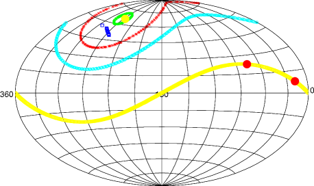
Figure 2: The distribution of the pointings used in this paper is shown in the J2000 mean equator coordinate system by the blue squares. The LUT’s available sky is located between the red and green circles. The locus of the zenith of LUT is shown by the cyan curve. The large yellow point marks the north pole of the Moon. The solid yellow line shows the equator in ecliptic. The locations of the Sun in April 10th, 2014 and June 8th, 2014 are marked by the large red points.

LUT has been successfully launched on December $2^{\mathrm{nd}}$, 2013 by a Long March-3B rocket, and had its first light on December $16^{\mathrm{th}}$, 2013, two days after the CE-3 lander landed on the lunar surface at 19.51˚W and 44.12˚N. With the location on the Moon and the scope of the gimbal, LUT can cover the sky region around the north pole of the Moon with a total area about 3600degrees² (see Figure 2 as an illustration). By the end of December 2014, LUT has smoothly worked on the Moon for an earth year, and acquired a total of more than 130,000 images. Its first six months of operation shows a highly stable photometric performance (Wang et al. 2015).

Figure 1 shows the measured throughput as a function of wavelength for the whole system. The throughput peaks at 2500Å with a peak value of $\approx 8\%$ and has an effective full width at half maximum (FWHM) of 1080Å. The throughput has been determined in the laboratory at pre-launch by a dedicated calibration system. The system is composed of a deuterium lamp, a halogen-tungsten lamp, a 207D type monochromator from McPherson, Inc., an adjustable diaphragm and two pre-calibrated sensors. The telescope collects the collimated output light from the monochromator without any intervening optics element on the light path.

3 Observations

A series of 498 images with extremely low stray light level were obtained by LUT when it performed a survey observation and a monitor on RR Lyr type variable star XZ Cyg ($\alpha=\mathrm{19^{h}:32^{m}:29^{s}.3}$, $\delta=\mathrm{+56\char 23\relax:23^{\prime}:17^{\prime\prime}}$, J2000) in April 10th, 2014 and June 8th, 2014, respectively. All the images were taken with an exposure time of 30 seconds. The telescope pointing was fixed with respect to the Moon within each exposure. The shift of a star on the focal plane within each exposure is negligible compared with the size of the point-spread-function (PSF). In the monitor, the diurnal apparent motion of the stars was compensated by a step tracking with an interval less than 30 minutes, which enables the star to have a significant shift with respect to the fixed stray light pattern caused by the sunshine. LUT changed its pointing in very 30 minutes in the survey observation for the same reason. The survey images used in this paper were taken at a sky region roughly at $\alpha=\mathrm{17^{h}30^{m}-18^{h}30^{m}}$, $\delta=\mathrm{+50-+55\char 23\relax}$. The distribution of all the used pointings is shown in Figure 2. The elevation of the Sun was about 12-13˚ when these images were taken.

4 Data Reductions

4.1 Image reductions

The raw 498 images were reduced through standard procedures in astronomy by the IRAF package, including overscan correction, bias and dark current subtraction, and flat filed normalization. The bias and dark current images were obtained at the beginning and end of each lunar day. All the 498 images and the bias and dark current images were taken at a fixed CCD temperature of -40˚C.

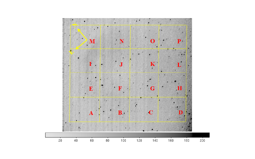
Figure 3: An example of the reduced and combined image. The combined image was taken in the survey observation in April 10th, 2014. The center of the image is at $\alpha=\mathrm{18^{h}:00^{m}:08^{s}.6}$, $\delta=\mathrm{+51\char 23\relax:22^{\prime}:09^{\prime\prime}}$ (J2000). The size of the image is about $1.35\times 1.35\mathrm{degrees^{2}}$. The east and north directions are marked by the two yellow arrows labeled at the left-upper corner. The points in the image are stars, and the strips at the left side are due to the CCD electronics. The bar underneath the image shows the scale of variation of brightness in logarithm. A pattern due to the stray light caused by the sunshine can be identified from a ring around the image center and from a gradual brightening at the CCD right fringe. The horizontal and vertical yellow lines illustrate the grid used to separate the image into 16 sub-images each with a pixel size of $200\times 200$.

The instrumental effect removed images were divided into 23 groups according to the pointing of the telescope, i.e., the pointing is fixed with respect to the Moon for each of the groups. The total time of each group was additionally required to be no more than 30 minutes. The level and pattern of the stray light caused by the sunshine is therefore believed to be stable for each group, because both pattern and level of the stray light change with time and with telescope pointing with respect to the Moon. The images in each group were then combined to enhance the signal-to-noise (S/N) ratio of the background. The median value of each pixel was extracted in the image combination. One combined image is shown in Figure 3 as an example. Each combined image was subsequently smoothed by a box with a size of 5$\times$5 pixels by using the IRAF package to further enhance its background S/N ratio.

4.2 Pixel distributions

The aim of this study is to estimate the content of the sunshined lunar exosphere from the diffuse sky background caused by the resonant line emitted from the species in the exosphere. This task is, however, complicated by several issues. At first, although the stray light level is extremely low in the 498 images, a stray light pattern can still be clearly identified in all these images (see Figure 3 as an example again), which results in a nonuniform contamination on the potential diffuse background caused by the resonant line emission. Secondly, both pattern and level of the stray light vary with both time and pointing with respect to the Moon. Finally, the contamination caused by the stray light can not be entirely excluded from the images.

To address the first issue, we divided each combined and smoothed image into 16 sub-images each with a physical size of 200$\times$200 pixels (see an illustration of the grid and the identification of each of the sub-images in Figure 3). A pixel distribution was extracted from each sub-image. Generally speaking, each distribution shows a strong peak superposed by a secondary peak or a tail at its large count-rate end. Our examination by eyes indicated that both the secondary peak and the large count-rate wing are likely resulted from the pollution caused by the stray light pattern. We then fitted each of the distributions by a sum of multiple Gaussian functions. The fitting is schemed in Figure 3 for two typical distributions extracted from different sub-images (i.e., different sub-image identifications) that were taken at different time with different pointings with respect to the Moon. The diffuse background level of each sub-image was determined from the fitted expected value of the Gaussian function that reproduces the strong peak of the distribution.

In a given combined image, its underlying diffuse background level with minimized stray light contamination was extracted from the 16 diffuse background levels determined at different CCD regions by the lowest one. Table 1 lists these values for the 23 combined and smoothed images. For each of the combined images, the Column (3) lists the count rate of its diffuse background along with the corresponding uncertianty at 1$\sigma$ significance level. The reported count rate was converted from the originally recorded ADU by using a measured CCD gain of 1.59. The uncertainty was obtained from the fitted width of the Gaussian function. The corresponding S/N ratio and the identification of the sub-image in which the diffuse background level was measured are tabulated in Column (5) and (2), respectively. One can see from the Column (5) that the lowest stray light contamination always occurs at the two left corners of the CCD in all the 23 combined images, which is in agree with our inspection by eyes.

As shown by the Column (3) in Table 1, one can see a considerable variation of the determined diffuse background count rates. The variation can be easily understood because these combined images were taken at different time with different pointings with respect to the Moon. In order to further minimize the stray light contamination, the lowest diffuse background level with a count rate of $\mathrm{0.096\pm 0.024e^{-}\ s^{-1}\ pixel^{-1}}$ (with a S/N ratio of 3.96) is adopted in the subsequent calculations. The value was derived from the sub-image B in the combined image No. 31.

Finally, we emphasize that this adopted value should be used as an upper limit of the diffuse background level caused by the resonant line emission, because the contamination due to the stray light can not be fully removed from the observed background.

5 Transformation from the Background to Atmosphere Content

One should be bear in mind that the lowest diffuse background count rate of $\mathrm{0.096\pm 0.024e^{-}\ s^{-1}\ pixel^{-1}}$ derived above contains the contributions from: 1) the stray light caused by the sunshine; 2) the zodiacal light from the solar system, and 3) the emission from the resonant transitions in the lunar exosphere. These complications result in the fact that only an upper limit of the content of a given species can be inferred from the LUT’s in-situ measurements. The potential transitions within the LUT’s wavelength coverage includes the $\mathrm{OH(0-0)(A^{2}\Sigma^{+}-X^{2}\Pi)}$ at 3087Å, MgI$\lambda$2853 and AlI$\lambda 3092$ (Morgan & Killen, 1997, see below).

5.1 Contribution from the zodiacal light

We estimated the underlying contribution from the zodiacal light in the LUT bandpass through a combination of the zodiacal map, the zodiacal spectral shape (both taken from Leinert et al., 1998) and the throughput of LUT. The count rate due to the zodiacal light can be calculated through the integration of

$$R_{\mathrm{ZL}}=\frac{1}{4}\pi d^{2}\Delta\Omega\int I_{\lambda}^{\mathrm{ZL}}(\beta-\beta_{\odot},\lambda^{\prime})S_{\lambda}d\lambda$$ (1)

where $d=150$mm is the diameter of the aperture of LUT, $S_{\lambda}$ the system throughput at different wavelengths, and $\Delta\Omega=22.7\mathrm{arcsec^{2}\ pixel^{-1}}$ the solid angle of each pixel. $I_{\lambda}^{\mathrm{ZL}}(\beta-\beta_{\odot},\lambda^{\prime})$ is the spectrum of the surface brightness of the zodiacal light measured at the Earth, whose shape and absolute level are a function of the viewing direction ($\beta-\beta_{\odot}$, $\lambda^{\prime}$) with respect to the Sun. A fixed spectral shape that is best measured at the ecliptic equator with a solar elongation $\beta-\beta_{\odot}=90$˚ was adopted in our integration. The absolute intensity of the spectrum was determined from the zodiacal map by a 2-dimensional interpolation. With the calculated viewing direction of $\beta-\beta_{\odot}\sim 110\char 23\relax$ and $\lambda^{\prime}\sim 75\char 23\relax$ (see Figure 2 as an illustration), the count rate on the focal plane caused by the zodiacal light was finally estimated to be $R_{\mathrm{ZL}}\sim 0.02\mathrm{e^{-}\ pixel^{-1}\ s^{-1}}$.

5.2 Lunar exosphere content

5.2.1 Method

A corrected diffuse background count rate of $R\sim 0.08\pm 0.02\mathrm{e^{-}\ s^{-1}\ pixel^{-1}}$ was finally derived after the exclusion of the estimated contribution due to the zodiacal light. By assuming this background count rate is entirely caused by the resonant scattering line emission (within the LUT bandpass) of a given species in the lunar exosphere, an upper limit of the column density $N$ of the species can be calculated as follows.

At the beginning, the diffuse background count rate $R$ was transformed to the resonant line intensity $I_{s}$ as

$$R=\frac{1}{4}\pi d^{2}S_{\lambda}\Delta\Omega I_{s}$$ (2)

where $S_{\lambda}$ is the measured throughput of LUT at the line wavelength of $\lambda$. The calculated line intensity was subsequently used to estimate the column density $N$ of the species in the optical thin case (Flynn & Stern, 1996):

$$4\pi I_{s}\cos\theta=gN$$ (3)

where $\theta\sim 37\char 23\relax$ is a parameter accounting for the angular distance from the pointing of LUT to the local zenith, and $g$ the corresponding fluorescence efficiency at 1AU (i.e., the g-factor). The g-factor is defined as an emission probability per atom in units of $\mathrm{photon\ s^{-1}\ atom^{-1}}$, and is determined by summing the probabilities of all transitions from multiple states whose population partitions are solved from the detailed equilibrium of every state that is usually not in thermodynamic equilibrium.

5.2.2 OH radicals

Taking the g-factor of $g=2.3\times 10^{-4}\ \mathrm{photons\ s^{-1}\ molecule^{-1}}$ (Schleicher et al., 1988) at 1AU for the OH 3087Å transitions, the zodical light-corrected diffuse background count rate of $R\sim 0.08\pm 0.02\mathrm{e^{-}\ pixel^{-1}\ s^{-1}}$ was transferred to an upper limit of the column density of $N\sim(6.0\pm 1.5)\times 10^{11}\ \mathrm{cm^{-2}}$ for the OH radicals. A slightly lower upper limit of $N\sim(4.0\pm 1.0)\times 10^{11}\ \mathrm{cm^{-2}}$ can be obtained if the g-factor at a temprature of 200K of $g=3.5\times 10^{-4}\ \mathrm{photons\ s^{-1}\ molecule^{-1}}$ (Stevens et al., 1999) was adopted in the calculation.

We transformed the calculated column density to the surface concentration $n_{0}$ as $N=n_{0}\Delta H$ by assuming a hydrostatic equilibrium, where $\Delta H$ is the model dependent scale height of the vertical density profile. The light OH radicals are believed to be thermal released (Stern, 1999). By adopting a typical scale height of $\Delta H=100\mathrm{km}$ (Wurz et al., 2007), two comparable surface concentrations of $\sim(6.0\pm 1.5)\times 10^{4}\ \mathrm{cm^{-3}}$ and $\sim(4.0\pm 1.0)\times 10^{4}\ \mathrm{cm^{-3}}$ can be obtained from the two estimated column densities, which depends on the adopted g-factor values. The slight difference between the two adopted g-factor values enables us to report an upper limit of the surface OH concentration of $\sim 10^{4}\ \mathrm{cm^{-3}}$, which is the best constraint on the OH content in the lunar exosphere to date (see a comparison in the next section). The calculated results are summarized in Table 2. The total mass of the OH radicals in the exosphere was estimated to be no more than $\sim 1.5\times 10^{3}\ \mathrm{kg}$.

5.2.3 Neutral magnesium and aluminum

Besides the OH resonant emission at 3087Å, the LUT bandpass covers two strong resonant emission lines, they are MgI$\lambda$2853 and AlI$\lambda$3092 (Morgan & Killen, 1997). We calculated the upper limits of both column density and surface concentration for the two species by the same method described in Section 5.2.1.

Using the g-factor value of the MgI$\lambda$2853 resonant line emission of $2.3\times 10^{-4}\ \mathrm{photons\ s^{-1}\ atom^{-1}}$ reported in Morgan & Killen (1997), we derived an upper limit of the column density of the neutral magnesium of $\sim(2.0\pm 0.5)\times 10^{9}\ \mathrm{cm^{-2}}$ from the zodiacal light-corrected diffuse background count rate of $R\sim 0.08\pm 0.02\mathrm{e^{-}\ pixel^{-1}\ s^{-1}}$. The assumption of a hydrostatic equilibrium yielded an upper limit of the surface concentration of $\sim(2.0\pm 0.5)\times 10^{2}\ \mathrm{cm^{-2}}$ when a scale height of 100km is adopted. Ion sputter model shows that the heavy atoms like Mg and Al can reach a considerably large scale height of $\sim 1,000\ \mathrm{km}$ due to the sputtering by the solar wind (Wurz et al., 2007). If so, the inferred surface concentration is $<20\pm 5\ \mathrm{cm^{-2}}$ for the neutral magnesium. It is noted that both upper limits of the surface concentration obtained with different scale height values are lower than those reported in the previous studies (see a comparison in the next section).

An upper limit of the column density of the neutral aluminum was calculated to be $\sim(4.0\pm 1.0)\times 10^{9}\ \mathrm{cm^{-2}}$ based on the g-factor of the AlI$\lambda$3092 resonant line emission of $3.8\times 10^{-2}\ \mathrm{photons\ s^{-1}\ atom^{-1}}$ (Morgan & Killen 1997). The inferred surface concentration is $<(4.0\pm 1.0)\times 10^{2}\ \mathrm{cm^{-3}}$ for a scale height of 100km, and $<40\pm 10\ \mathrm{cm^{-3}}$ for a scale height of 1,000km.

All these calculated results are tabulated in Table 2. Note that the surface concentrations listed in the table are all based on a scale height of 100 km.

6 Comparisons

The extremely low density of the lunar exosphere results in a considerable challenge in determining its content. The current study shows that the LUT’s in-situ measurements provide the best constraints on the content of the lunar exosphere to date, both because of the high efficiency of LUT and because of the avoidance of the contamination caused by the instrument itself.

The upper limit of $<10^{4}\ \mathrm{cm^{-3}}$ derived for the OH radicals is lower than that derived from the HST low resolution spectroscopy (i.e, $<10^{6}\mathrm{cm^{-3}}$, Stern et al., 1997) by about two orders of magnitude, and is lower than that inferred from the mass spectra taken by the Chandrayaan-1 mission (see Introduction and Wang et al. (2011) for the details) by about 6 orders of magnitude.

We argue that the upper limit derived from the LUT’s in-situ measurements is very close to the prediction of the ion sputtering model. The chemically adsorbed $\mathrm{H_{2}O/OH}$ molecules (Stern, 1999; Starukhina et al., 2000; Arnold, 1979) could be sputtered by the solar wind protons, which produces water vapor and gaseous OH radicals in the exosphere through chemical reactions (e.g., Morgan et al., 1997; Wurz et al., 2007; Killen & Ip, 1999; Hunten et al., 1997; Johnson et al., 1991; Killen et al., 1999). The sputtering results in a surface $\mathrm{H_{2}O/OH}$ concentration $n_{0}\sim f_{a}j\eta\upsilon^{-1}\sim 10^{3}\ \mathrm{cm^{-3}}$, where $j\sim 10^{8}\ \mathrm{p^{+}\ cm^{-2}\ s^{-1}}$ is the proton flux of the solar wind, $\eta\sim 0.1$ the production rate per proton (Crider & Vondrak, 2002), $\upsilon\sim 10^{2}\ \mathrm{m\ s^{-1}}$ the typical velocity of a particle, and $f_{a}\sim 0.8$ the fraction of the solar protons that are absorbed at the lunar surface. Recent observations carried out by Chandrayaan-1/SARA (Sub-kev Atom Reflection Analyzer) found that about $\sim 20\%$ of the incident solar protons is backscattered to space from the surface (Bhardwaj et al., 2012). The backscattered proton becomes a hydrogen atom by recombining with an electron.

Previous study reported an upper limit of $<6,000\ \mathrm{cm^{-3}}$ at a significance level of 5$\sigma$ for the neutral magnesium (Stern et al., 1997), which is larger than the value reported in this study by about two (for $\Delta H=100\mathrm{km}$) or three (for $\Delta H=1000\mathrm{km}$) orders of magnitude. HST UV spectroscopy observation reported a 5$\sigma$ upper limit of $<11,000\mathrm{cm^{-3}}$ for neutral aluminum. This value is larger than that given by the LUT’s measurements by about two orders of magnitude, when a scale height of 100km was adopted in our calculations. A much lower upper limit of $<55\mathrm{cm^{-3}}$ at a significance level of 5$\sigma$ was obtained from the ground-based spectroscopy (Flynn & Stern, 1996), which is very close to the upper limit derived here when a scale height of $\Delta H=1000\mathrm{km}$ was used.

7 Conclusions

An unprecedented upper limit of the OH (MgI) content in the lunar exosphere is obtained from the in-situ measurements carried out by LUT. The inferred column density and surface concentration are $<10^{11}\ \mathrm{cm^{-2}}$ and $<10^{4}\ \mathrm{cm^{-3}}$ for the OH radicals, respectively, which is close to the value predicted by the sputtering model. In addition, a surface concentration of $<10^{2}\ \mathrm{cm^{-3}}$ is obtained for neutral magnesium from the same measurements and method.

Figure 1: The normalized throughput of LUT plotted against wavelength.

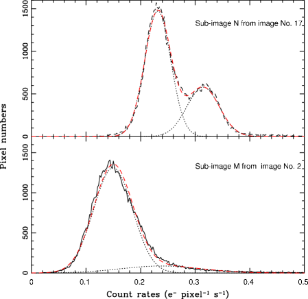
Figure 4: Examples of fitting an extracted pixel distribution by a sum of two Gaussian functions. In each panel, the observed distribution and the best fit curve are plotted by the black solid and red dashed lines, respectively. The two fitted Gaussian functions are shown by the dotted lines.

Table 1: The determined underlying background count rates of the 23 combined images.

Combined image ID	sub-image ID	count-rate	S/N
		$\mathrm{e^{-}s^{-1}pixel^{-1}}$
(1)	(2)	(3)	(4)
02	M	$0.150\pm 0.036$	4.21
03	M	$0.195\pm 0.032$	6.07
04	M	$0.201\pm 0.032$	6.28
07	M	$0.169\pm 0.030$	5.64
08	M	$0.154\pm 0.029$	5.35
09	M	$0.136\pm 0.028$	4.78
12	M	$0.276\pm 0.029$	9.53
13	M	$0.391\pm 0.030$	13.25
15	N	$0.291\pm 0.026$	11.20
16	M	$0.350\pm 0.026$	13.59
17	N	$0.231\pm 0.024$	9.66
18	N	$0.172\pm 0.022$	7.91
20	N	$0.224\pm 0.022$	10.15
21	N	$0.170\pm 0.019$	8.98
22	N	$0.172\pm 0.020$	8.54
23	M	$0.191\pm 0.027$	6.98
24	M	$0.182\pm 0.027$	6.69
25	M	$0.144\pm 0.025$	5.76
26	M	$0.158\pm 0.027$	5.83
28	M	$0.106\pm 0.027$	3.91
29	M	$0.118\pm 0.029$	4.10
31	B	$0.096\pm 0.024$	3.96
32	E	$0.164\pm 0.032$	5.04

Table 2: Calculated column densities and surface concentrations for different species.

Species	Wavelength	N	$n_{0}$	g-factor @ 1AU	Reference
	Å	$\mathrm{cm^{-2}}$	$\mathrm{cm^{-3}}$	$\mathrm{photons\ s^{-1}\ molecule^{-1}}$
(1)	(2)	(3)	(4)	(5)	(6)
MgI	2853	$(2.0\pm 0.5)\times 10^{9}$	$(2.0\pm 0.5)\times 10^{2}$	$5.4\times 10^{-2}$	Morgan & Killen (1997)
OH	3087	$(6.0\pm 1.5)\times 10^{11}$	$(6.0\pm 1.5)\times 10^{4}$	$2.3\times 10^{-4}$	Schleicher et al. (1988)
		$(4.0\pm 1.0)\times 10^{11}$	$(4.0\pm 1.0)\times 10^{4}$	$3.5\times 10^{-4}$	Stevens et al. (1999)
AlI	3092	$(4.0\pm 1.0)\times 10^{9}$	$(4.0\pm 1.0)\times 10^{2}$	$3.8\times 10^{-2}$	Morgan & Killen (1997)

References

- Arnold (1979) Arnold, J. R. Ice in the lunar polar regions. JGR 84, 5659-5668, 1979
- Bhardwaj et al. (2012) Bhardwaj, A., Dhanya, M. B., Sridharan, R., et al. Interaction of Solar Wind with Moon: AN Overview on the Results from the SARA Experiment Aboard CHANDRAYAAN-1. Advances in Geosciences, Planetary Science (PS) and Terrestrial Science (TS) 30, 35, 2012
- Cao et al. (2011) Cao, L., Ruan, P., Cai, H. B., et al. LUT: A Lunar-based Ultraviolet Telescope. ScChG 54, 558-562, 2011
- Clark (2009) Clark, R. N. Detection of Adsorbed Water and Hydroxyl on the Moon. Science 326, 562-564, 2009
- Crider & Vondrak (2002) Crider, D. H., Vondrak, R. R. Hydrogen migration to the lunar poles by solar wind bombardment of the Moon. AdSpR 30, 1869-1874, 2002
- Crovisier (1989) Crovisier, J. The photodissociation of water in cometary exospheres. A&A 213, 459-464, 1989
- Dyar et al. (2010) Dyar, M. D., Hibbitts, C. A., Orlando, T. M. et al. Mechanisms for incorporation of hydrogen in and on terrestrial planetary surfaces. Icar 208, 425-437, 2010
- Feldman & Morrison (1991) Feldman, P. D. & Morrison, D. The Apollo 17 Ultraviolet Spectrometer-Lunar atmosphere measurements revisited. GeoRL 18, 2105-2108, 1991
- Flynn & Stern (1996) Flynn, B.C. & Stern, S.A. A Spectroscopic Survey of Metallic Species Abundances in the Lunar Atmosphere. Icar 124, 530-536, 1996
- Heiken et al. (1991) Heiken, G. Vaniman, D., French, B. M. LUNAR SOURCEBOOK: A User’s Guide to the Moon I. Cambridge University Press, 1991
- Hibbitts et al. (2010) Hibbitts, C. A., Dyar, M. D., Orlando, T. M., et al. Thermal stability of water and hydroxyl on airless bodies. LPI 41, 2417-2418, 2010
- Hodges (1973) Hodges, Jr. R. R. Helium and hydrogen in the lunar exosphere. JGR 78(34), 8055-8064, 1973
- Hodges et al. (1972) Hodges, Jr. R. R., Hoffman, J. H., Yeh, T. T. J., et al. Orbital search for lunar volcanism. JGR 73(23), 7307-7317, 1972
- Ip et al. (2014) Ip, W -H., Yan, J., Li, C -L. Ouyang, Z -Y. Preface: The Chang’e-3 lander and rover mission to the Moon. RAA 14, 1511-1513, 2014
- Johnson et al. (1972) Johnson, F.S., Carroll, J.M.,& Evans, D.E. Lunar atmosphere measurements. Proceedings of the Lunar Science Conference 2, 2231-2242, 1972
- Killen & Ip (1999) Killen, R.M., Ip, W.-H. The surface-bounded exospheres of Mercury and the Moon. Rev. Geophys 37(3), 361-406, 1999
- Kolowski et al. (1990) Kozlowski, R. W. H., Sprague, A. L., & Hunten, D. M. Observations of potassium in the tenuous lunar atmosphere. GeoRL 17, 2253-2256, 1990
- Killen et al. (1999) Killen, R. M., Potter, A., Fitzsimmons, A., et al. Sodium D2 line profiles: clues to the temperature structure of Mercury’s exosphere. P&SS 47, 1449-1458, 1999
- Leinert et al. (1998) Leinert, C., et al. The 1997 reference of diffuse night sky brightness. A&A, 127, 1-99, 1998
- Morgan & Killen (1997) Morgan, T. H., Killen, R. M. C. A non-stoichiometric model of the composition of the exospheres of Mercury and the Moon. P&SS 45, 81-94, 1997
- Pieters et al. (2009) Pieters,C.M., et al. Character and Spatial Distribution of on the Surface of the Moon Seen by M3 on Chandrayaan-1. Science 326, 568-572, 2009
- Potter & Morgan (1988) Potter, A. E., Morgan, T. H. Discovery of sodium and potassium vapor in the atmosphere of the moon. Science 241, 675-680, 1988
- Potter & Morgan (1991) Potter, A. E., Morgan, T. H. Observations of the lunar sodium exosphere. GeoRL 18, 2089-2092, 1991
- Schleicher & AHearn (1988) Schleicher, D. G., AHearn, M. F. The fluorescence of cometary OH. ApJ 331, 1058-1077, 1988
- Sprague et al. (1992) Sprague, A. L., Kozlowski, R. W. H., Hunten, D. M., et al. The sodium and potassium atmosphere of the moon and its interaction with the surface. Icar 96, 27-42, 1992
- Sridharan et al. (2010a) Sridharan, R., Ahmed, S. M., Pratim. D., et al. Direct’ evidence for water () in the sunlit lunar ambience from CHACE on MIP of Chandrayaan I. P&SS 58, 947-950, 2010
- Sridharan et al. (2010b) Sridharan, R,, Ahmed, S. M., Pratim. D., et al. The sunlit lunar exosphere: A comprehensive study by CHACE on the Moon Impact Probe of Chandrayaan-1. P&SS 58, 1567-1577, 2010
- Stern (1999) Stern, S. A. The lunar exosphere: History, status, current problems, and context. RvGeo 37, 453-492, 1999
- Stern et al. (1997) Stern, S. A., Parker, J. W., Morgan, T. H., et al. NOTE: an HST Search for Magnesium in the Lunar Atmosphere. ICARUS 127, 523-526, 1997
- Stubbs et al. (2010) Stubbs, T. J., Glenar, D. A., Colaprete, A., et al. Optical scattering processes observed at the moon: Predictions for the LADEE ultraviolet spectrometer. P&SS 58, 830-837, 2010
- Sunshine et al. (2009) Sunshine,J. M., Farnham, T. L., Feaga, L. M., et al. Temporal and Spatial Variability of Lunar Hydration As Observed by the Deep Impact Spacecraft. Science 326, 565-568, 2009
- Tyler et al. (1988) Tyler, A. L., Hunten, D. M., & Kozlowski, R. W. H. Observations of sodium in the tenuous lunar atmosphere. GeoRL 15, 1141-1144, 1988
- Wang et al. (2011) Wang, J., Deng, J.S., Cui, J., Cao, L., Qiu, Y.L., & Wei, J.Y. Lunar exosphere influence on lunar-based near-ultraviolet astronomical observations. AdSpR, 48, 1927-1934, 2011
- Wang et al. (2015) Wang, J., Cao, L., Meng, X. M., et al. Photometric Calibration on Lunar-based Ultraviolet Telescope for Its First Six Months of Operation on Lunar Surface. RAA, 2015 in print
- Wen et al. (2014) Wen, W -B., Wang, F., Li, C -L., et al. Data preprocessing and preliminary results of the Moon-based Ultraviolet Telescope on the CE-3 lander. RAA 14, 1674-1681, 2014
- Wurz et al. (2007) Wurz, P., Rohner, U., Whitby, J. A., et al. The lunar exosphere: The sputtering contribution. ICARUS 191, 486-496, 2007